Adaptation and Robust Learning
of Probabilistic Movement Primitives

Abstract

Probabilistic representations of movement primitives open important new possibilities for machine learning in robotics. These representations are able to capture the variability of the demonstrations from a teacher as a probability distribution over trajectories, providing a sensible region of exploration and the ability to adapt to changes in the robot environment. However, to be able to capture variability and correlations between different joints, a probabilistic movement primitive requires the estimation of a larger number of parameters compared to their deterministic counterparts, that focus on modeling only the mean behavior. In this paper, we make use of prior distributions over the parameters of a probabilistic movement primitive to make robust estimates of the parameters with few training instances. In addition, we introduce general purpose operators to adapt movement primitives in joint and task space. The proposed training method and adaptation operators are tested in a coffee preparation and in robot table tennis task. In the coffee preparation task we evaluate the generalization performance to changes in the location of the coffee grinder and brewing chamber in a target area, achieving the desired behavior after only two demonstrations. In the table tennis task we evaluate the hit and return rates, outperforming previous approaches while using fewer task specific heuristics.

I Introduction

Techniques that can learn motor behavior from human demonstrations and reproduce the learned behavior in a robotic system have the potential to generalize better to different tasks. Multiple models have been proposed to represent complex behavior as a sequence of simpler movements typically known as movement primitives. A movement primitive framework should provide operators to learn primitives from demonstrations, adapt them to achieve different goals and execute them in a sequence on a robotic system.

Deterministic Movement Primitive frameworks have been used successfully for a variety of robotic tasks including locomotion [1], grasping [2], ball in a cup [3] and pancake flipping [4]. However, deterministic representations capture only the mean behavior of the demonstrations of the teacher. The variability in the demonstrations is not captured nor used.

In biological systems, variability seems to be characteristic of all behavior, even in the most skilled and seemingly automated performance [5]. Thus, a movement primitive representation that captures variance in the demonstrated behavior has the potential to model the human teacher better. For a task like table tennis, the variability of the teacher is partially a response to the changes in ball trajectory. Therefore, approaches that capture it have the potential to adapt better to diverse ball trajectories. At the same time, the variability of the teacher can be used to define a region of sensible exploration for a robotic system.

Probabilistic approaches can naturally capture variability using a probability distribution. Some probabilistic representations of movement primitives focus on learning a distribution over demonstrated states using Gaussian Mixture models or Hidden Markov models [6][7]. Subsequently using the log-likelihood as cost function to reproduce the learned movement using an optimal control method [8][9].

Other probabilistic representations focus on learning a distribution over robot trajectories directly. Some approaches represent trajectories as functions of time and the distribution over these trajectories using parametric [10] or non-parametric [11] approaches. The trajectories can also be represented with recursive probability distributions, using latent state space models [12].

In this paper, we build on top of a probabilistic representation introduced in [10] called Probabilistic Movement Primitives (ProMPs). In this probabilistic formulation of movement primitives, a movement primitive is represented as a probability distribution over robot trajectories. Different realizations of the same movement primitive are assumed to be independent samples from the distribution over trajectories.

Figure 1: Robot table tennis setup used to evaluate the proposed methods. The ball is tracked using four cameras attached to the ceiling. The robot arm is a Barrett WAM capable of high speed motion, with seven degrees of freedom like a human arm.

ProMPs have typically more parameters than non-probabilistic representations. These extra parameters are used to capture the variability of the movements executed by the teacher and the correlations between different degrees of freedom of the robot. In this paper, we use prior distributions over the ProMP parameters to make robust estimates with few demonstrations. The influence of the prior distribution decreases as more training data becomes available, converging to the maximum likelihood estimates.

This paper also presents general purpose operators to adapt a ProMP to have a desired joint or task space configuration at a certain time. By joint space we refer to the joint angles and velocities of the robot, and by task space we refer to the world coordinate position and velocity of the end effector of the robot.

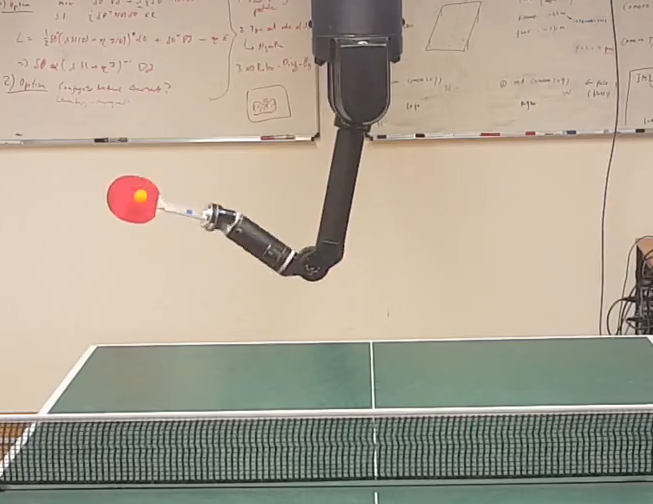
The proposed method to learn the movement primitive and the operators to adapt the movement primitives in task and joint space are evaluated with synthetic data, in a robot table tennis task and a robot assisted coffee preparation task. Figure 1 shows the robot table tennis setup used in the experiments. The results obtained with the presented method are compared with previous work on robot table tennis. The proposed approach outperforms previous robot table tennis approaches using less task specific heuristics. Examples of task specific heuristics used for robot table tennis in previous approaches include using a Virtual Hitting Planes [13] and computing optimal racket velocity and orientation at hitting time to send balls to the opponent side of the table [14]. The presented approach does not compute racket orientations or velocities to return balls to the opponent’s court. The training data used to learn the movement primitives was built using only successful human demonstrations. The robot was able to learn the behavior required to successfully return balls to the opponent side of the table from the human demonstrations.

We use the pouring coffee task to evaluate the generalization performance of the presented method as a function of the number of training instances by changing the position of the coffee grinder and the brewing chamber. The robot manages to pour successfully on the selected testing area after two training demonstrations, suggesting that the presented prior is a sensible choice for this task. Finally, the fact that the presented approach can be used for two robot tasks as different as table tennis and coffee pouring without any changes suggests it has the potential to perform well in several other robot applications.

II Robust Learning of Probabilistic Movement Primitives

Figure 2: Probabilistic Movement Primitive graphical model. The joint state $\boldsymbol{y}_{nt}$ is generated from the compact representation of a trajectory $\boldsymbol{\omega}_{n}$ using (1). The mean behavior of the different trajectories is represented by the variable $\boldsymbol{\mu}_{\omega}$. The variability of the teacher and the correlations between different joints are represented by $\boldsymbol{\Sigma}_{\omega}$. Each trajectory $\boldsymbol{\omega}_{n}$ is generated using (2). The number of trials is denoted by $N$, and the number of time steps of the trial $n$ is denoted by $\mathrm{T}_{n}$.

Probabilistic movement primitives (ProMPs) are probability distributions used to represent motion trajectories [10]. A trajectory $\tau=\{\boldsymbol{y}_{t}\}_{t=1}^{T}$, can be represented as positions or joint angles at different moments in time. In this paper, we assume that $\boldsymbol{y}_{t}$ is a $D$ dimensional vector that represents the joint measurement at time $t$ of a robotic system with $D$ degrees of freedom.

First, let us introduce a variable $\boldsymbol{\omega}={[{\boldsymbol{\omega}_{1}}^{\top},\dots,{\boldsymbol{\omega}_{D}}^{\top}]}^{\top}$ that encodes compactly a single robot trajectory, and consists of the concatenation of $D$ weight vectors $\boldsymbol{\omega}_{d}$ that represent the trajectory of each of the degrees of freedom of the robot, indexed by $d$.

Given a trajectory realization represented by $\boldsymbol{\omega}$, the joint state at time $t$ is computed as

$$\boldsymbol{y}_{t}={[{\boldsymbol{\phi}_{1}(t)}^{\top}\boldsymbol{\omega}_{1},\cdots,{\boldsymbol{\phi}_{D}(t)}^{\top}\boldsymbol{\omega}_{D}]}^{\top}+\boldsymbol{\epsilon}_{y},$$

where the vector $\boldsymbol{\phi}_{d}(t)$ is a computed from a set of time dependent basis functions, and $\boldsymbol{\epsilon}_{y}$ is Gaussian white noise. To obtain smooth trajectories, the basis functions need to be smooth. In this paper we use radial basis functions (RBF), polynomial basis functions and a combination of both. The number and type of basis functions to use is a design choice. Each degree of freedom could have a different number of basis functions, but for simplicity we assume every degree of freedom uses $K$ basis functions.

The distribution over the values of the joint state at time $t$, can be written as

$$p(\boldsymbol{y}_{t}|\boldsymbol{\omega})=\mathcal{N}\left({\boldsymbol{y}_{t}}\,\left|\,{\boldsymbol{\Phi}_{t}\boldsymbol{\omega}},{\boldsymbol{\Sigma}_{y}}\right.\right),$$ (1)

where $\boldsymbol{\Phi}_{t}$ is a $D\times KD$ matrix used to write the distribution over $\boldsymbol{y}_{t}$ in vectorized form, and is defined as

$$\boldsymbol{\Phi}_{t}=\begin{pmatrix}\boldsymbol{\phi}_{1}(t)&\cdots&\boldsymbol{0}\\ \vdots&\ddots&\vdots\\ \boldsymbol{0}&\cdots&\boldsymbol{\phi}_{D}(t)\end{pmatrix}.$$

Different realizations of a movement primitive are assumed to have different values for $\boldsymbol{\omega}$. In this model, a particular realization $n$ represented by $\boldsymbol{\omega}_{n}$ is assumed to be sampled from

$$p(\boldsymbol{\omega}_{n}|\boldsymbol{\theta}_{\omega})=\mathcal{N}\left({\boldsymbol{\omega}_{n}}\,\left|\,{\boldsymbol{\mu}_{\omega}},{\boldsymbol{\Sigma}_{\omega}}\right.\right),$$ (2)

where $\boldsymbol{\theta}_{\omega}=\{\boldsymbol{\mu}_{\omega},\boldsymbol{\Sigma}_{\omega}\}$ is a set of parameters that capture the similarities and differences of different realizations of the movement primitive. In the rest of this section, we drop the index $n$ from $\boldsymbol{\omega}_{n}$ for notational simplicity.

Figure 3: Demonstrated trajectories and learned distribution for the first degree of freedom of Barrett WAM robot arm. The joint value $y_{0}$ corresponds to the shoulder yaw recorded in radians as a function of time. Different trajectories of a table tennis forehand motion are demonstrated by the human teacher. These trajectories are depicted in blue and have different durations. The duration of each trajectory is normalized to one to achieve duration invariance, the time invariant trajectories are depicted in green. The learned distribution is depicted in red. The shaded area corresponds to two standard deviations. Note that the model captures the mean behavior and the variability of the teacher at different points in time.

Let us write the distribution $p(\boldsymbol{\omega}|\boldsymbol{\theta}_{\omega})$ decomposing the $KD\times 1$ vector $\boldsymbol{\mu}_{\omega}$ and the $KD\times KD$ matrix $\boldsymbol{\Sigma}_{\omega}$ in the components corresponding to each degree of freedom,

$$\mathcal{N}\left({\begin{pmatrix}\boldsymbol{\omega}_{1}\\ \vdots\\ \boldsymbol{\omega}_{D}\\ \end{pmatrix}}\,\left|\,{\begin{pmatrix}\boldsymbol{\mu}_{\omega}^{1}\\ \vdots\\ \boldsymbol{\mu}_{\omega}^{D}\\ \end{pmatrix}},{\begin{pmatrix}\boldsymbol{\Sigma}_{\omega}^{(1,1)}&\cdots&\boldsymbol{\Sigma}_{\omega}^{(1,D)}\\ \vdots&\ddots&\vdots\\ \boldsymbol{\Sigma}_{\omega}^{(D,1)}&\cdots&\boldsymbol{\Sigma}_{\omega}^{(D,D)}\\ \end{pmatrix}}\right.\right).$$

Note that the mean behavior for the degree of freedom $d$ is captured by the $K\times 1$ vector $\boldsymbol{\mu}_{\omega}^{d}$ and the variability by the $K\times K$ matrix $\boldsymbol{\Sigma}_{\omega}^{(d,d)}$. The correlation between two different joints $d_{1}$ and $d_{2}$ is captured by $\boldsymbol{\Sigma}_{\omega}^{(d_{1},d_{2})}$. The model can be forced to consider all the joints independently by forcing the matrix $\boldsymbol{\Sigma}_{\omega}$ to be block diagonal.

A probabilistic graphical model is a probabilistic model for which a graph expresses conditional independence assumptions between random variables [15]. Figure 2 shows the graphical representation of the probabilistic model used to represent movement primitives. To sample a robot trajectory given the ProMP parameters $\boldsymbol{\mu}_{\omega}$ and $\boldsymbol{\Sigma}_{\omega}$, a vector $\boldsymbol{\omega}_{n}$ is sampled using (2). Subsequently, the new trajectory of length $\mathrm{T}_{n}$ can be sampled using (1). If the used basis functions are smooth, the sampled trajectories will also be smooth.

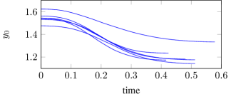
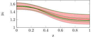
Figure 3 show six human demonstrations of a forehand table tennis striking movement and the learned probability distribution. The figure shows the value in radians of the shoulder yaw $y_{0}$ with respect to time. The original demonstrations given by the human teacher, depicted in blue, have different durations varying between 0.4 and 0.6 seconds. The time of every demonstration is normalized to be between zero and one to achieve duration invariance using a new variable $z=\frac{t-t0}{T}$, known as the phase variable [10]. The same demonstrations with respect to the phase variable are depicted in green, and the learned distribution is depicted in red. The shaded area corresponds to two standard deviations. The ProMP learned from the given demonstrations capture the mean behavior and the teacher variability in different points of time.

II-A Learning from Demonstrations

The parameters $\boldsymbol{\theta}_{\omega}$ can be learned from human demonstrations. Let us assume we have $N$ recorded human demonstrations, and extend the notation with an extra sub-index $n\in\{1..N\}$ identifying each demonstration. Thus, the variables $\boldsymbol{y}_{nt}$ and $\boldsymbol{\omega}_{n}$ represent the joint state of the $n$th trial at time $t$ and the compact representation of the $n$th trial respectively. The likelihood of the recorded data is given by

$$p(\boldsymbol{Y}|\boldsymbol{\theta}_{\omega})=\prod_{n=1}^{N}{\int{p(\boldsymbol{\omega}_{n}\,|\,\boldsymbol{\theta}_{\omega})\prod_{t=1}^{\mathrm{T}_{n}}{p(\boldsymbol{y}_{nt}\,|\,\boldsymbol{\omega}_{n})}d{\boldsymbol{\omega}_{n}}}},$$

where $\boldsymbol{Y}$ is the set of values $\boldsymbol{y}_{nt}$ for all the training instances. Note that evaluating the likelihood requires the computation of an integral over the hidden variables $\boldsymbol{\omega}_{n}$. Although the integral in this case can be computed in closed form, evaluating the resulting expression would cost cubic time over the trajectory lengths $\mathrm{T}_{n}$. Instead, we propose to use the expectation maximization algorithm to optimize the likelihood or posterior distribution with linear time costs over the trajectory lengths $\mathrm{T}_{n}$.

In [16], the ProMP parameters are estimated by first making a point estimate of the hidden variables with least squares, and subsequently finding their empirical mean and covariance matrix as the ProMP parameters. This estimation procedure makes intuitive sense and avoids computing integrals. However, the authors did not provide a mathematical intuition of how their estimation procedure relates to maximizing the marginal likelihood. In the Appendix II-C, we explain in detail the estimation method introduced in [16], and show that it is an special case of an approximation of the proposed EM algorithm to maximize the likelihood. The approximation consists of performing a single EM iteration and approximating the Gaussian distribution computed in the E-step with a Dirac delta distribution, ignoring the uncertainty over the estimates of the hidden variables.

In previous work [17], the parameters were learned maximizing the likelihood. However, maximizing the likelihood results in numerically unstable estimates for the parameters of the ProMP unless a very large number of demonstrations is available. In [17], the matrix $\boldsymbol{\Sigma}_{\omega}$ is forced to be block diagonal to deal with the numerical problems. As a result, the ProMP parameters could be robustly estimated, but the model becomes incapable of learning the correlation between the different joints of the robot arm.

In this paper, we use regularization to estimate the ProMP parameters in the form of a prior probability distribution $p(\boldsymbol{\theta}_{\omega})$. The posterior distribution over the ProMP parameters is given by

$$p(\boldsymbol{\theta}_{\omega}|\boldsymbol{Y})\propto p(\boldsymbol{\theta}_{\omega})p(\boldsymbol{Y}|\boldsymbol{\theta}_{\omega}).$$ (3)

We estimate the parameters $\boldsymbol{\theta}_{\omega}$ by maximizing the posterior distribution of (3) using the expectation maximization algorithm. This estimator is commonly known as Maximum A Posteriori (MAP) estimate.

The pseudo-code summarizing the training procedure is presented in Algorithm 1. Lines 8 and 9 correspond to the E-step and lines 11 to 15 correspond to the M-step. The values $\boldsymbol{\epsilon}_{nt}=\boldsymbol{y}_{nt}-\boldsymbol{\phi}_{nt}\overline{\boldsymbol{w}}_{n}$ are the residuals used to estimate the sensor noise.

1:Demonstration dataset containing the joint states and corresponding normalized time stamps $\boldsymbol{Y}=\{\boldsymbol{y}_{nt},z_{nt}\}$ and the prior parameters $k_{0},\boldsymbol{m}_{0},v_{0},\boldsymbol{S}_{0}$

2:The ProMP parameters $\boldsymbol{\mu}_{\omega}$, $\boldsymbol{\Sigma}_{\omega}$, $\boldsymbol{\Sigma}_{y}$

3:Compute matrices $\boldsymbol{\phi}_{nt}=\boldsymbol{\phi}(z_{nt})$ with the basis functions $\boldsymbol{\phi}$

4:Compute $L=\sum_{n=1}^{N}{\tau_{n}}$

5:Set some initial values for $\boldsymbol{\mu}_{\omega}$, $\boldsymbol{\Sigma}_{\omega}$, $\boldsymbol{\Sigma}_{y}$. We use $\boldsymbol{\mu}_{\omega}=\boldsymbol{0}$, $\boldsymbol{\Sigma}_{\omega}=\boldsymbol{I}$ and $\boldsymbol{\Sigma}_{y}=\boldsymbol{I}$.

6:while Not converged do

7:     for  $n\in\{1,\dots,N\}$  do

8:         $\boldsymbol{S}_{\omega}^{n}\leftarrow\left(\Sigma_{\omega}^{-1}+\sum_{t=1}^{\tau_{n}}{{\boldsymbol{\phi}_{nt}}^{\top}\boldsymbol{\Sigma}_{y}^{-1}\boldsymbol{\phi}_{nt}}\right)^{-1}$

9:         $\overline{\boldsymbol{w}}_{n}\leftarrow\boldsymbol{S}_{\omega}^{n}\left(\boldsymbol{\Sigma}_{\omega}^{-1}\boldsymbol{\mu}_{\omega}+\sum_{t=1}^{\tau_{n}}{{\boldsymbol{\phi}_{nt}}^{\top}\boldsymbol{\Sigma}_{y}^{-1}\boldsymbol{y}_{nt}}\right)$

10:     end for

11:     $\boldsymbol{\mu}_{\omega}^{*}\leftarrow\frac{1}{N}\left(\sum_{n=1}^{N}{\overline{\boldsymbol{w}}_{n}}\right)$

12:     $\boldsymbol{\mu}_{\omega}\leftarrow\frac{1}{N+k_{0}}\left(k_{0}\boldsymbol{m}_{0}+N\boldsymbol{\mu}_{\omega}^{*}\right)$

13:     $\boldsymbol{\Sigma}_{\omega}^{*}\leftarrow\frac{1}{N}{\sum_{n=1}^{N}{\left(\boldsymbol{S}_{\omega}^{n}+(\overline{\boldsymbol{w}}_{n}-\boldsymbol{\mu}_{\omega}){(\overline{\boldsymbol{w}}_{n}-\boldsymbol{\mu}_{\omega})}^{\top}\right)}}$

14:     $\boldsymbol{\Sigma}_{\omega}\leftarrow\frac{1}{N+v_{0}+KD+1}\left[\boldsymbol{S}_{0}+N\boldsymbol{\Sigma}_{\omega}^{*}\right]$

15:     $\boldsymbol{\Sigma}_{y}\leftarrow\frac{1}{L}\sum_{n=1}^{N}{\sum_{t=1}^{\tau_{n}}{\left[\boldsymbol{\epsilon}_{nt}{\boldsymbol{\epsilon}_{nt}}^{\top}+\boldsymbol{\phi}_{nt}\boldsymbol{S}_{\omega}^{n}{\boldsymbol{\phi}_{nt}}^{\top}\right]}}$

16:end while

17:return  $\boldsymbol{\mu}_{\omega}$, $\boldsymbol{\Sigma}_{\omega}$ and $\boldsymbol{\Sigma}_{y}$.

Algorithm 1 Expectation Maximization algorithm to train a ProMP from demonstrations

II-B Prior Distribution

We use a Normal-Inverse-Wishart as a prior distribution over the ProMP parameters $\boldsymbol{\mu}_{\omega}$ and $\boldsymbol{\Sigma}_{\omega}$, given by

$$p(\boldsymbol{\mu}_{\omega},\boldsymbol{\Sigma}_{\omega}) =\mathrm{NIW}\left({\boldsymbol{\mu}_{\omega},\boldsymbol{\Sigma}_{\omega}}\,|\,{k_{0}},{\boldsymbol{m}_{0}},{v_{0}},{\boldsymbol{S}_{0}}\right)$$

$$=\mathcal{N}\left({\boldsymbol{\mu}_{\omega}}\,\left|\,{\boldsymbol{m}_{0}},{\frac{1}{k_{0}}\boldsymbol{\Sigma}_{\omega}}\right.\right)\mathcal{W}^{-1}\left({\boldsymbol{\Sigma}_{\omega}}\,|\,{v_{0}},{\boldsymbol{S}_{0}}\right),$$

where $\mathcal{W}^{-1}\left({\boldsymbol{\Sigma}_{\omega}}\,|\,{v_{0}},{\boldsymbol{S}_{0}}\right)$ is an inverse Wishart distribution, used frequently as a prior for covariance matrices. The main reason why we decided to use a Normal-Inverse-Wishart prior for the ProMP model is because it is a conjugate prior, resulting in closed form updates for the parameters in the EM algorithm and simplifying the inference process. Furthermore, the parameters of this prior distribution have a simple interpretation. Lines 11 and 13 compute the Maximum Likelihood estimates (MLE) $\boldsymbol{\mu}_{\omega}^{*}$ and $\boldsymbol{\Sigma}_{\omega}^{*}$. Lines 12 and 14 compute the MAP estimates $\boldsymbol{\mu}_{\omega}$ and $\boldsymbol{\Sigma}_{\omega}$. Note that the MAP estimates are a weighted average of the MLE estimates $\boldsymbol{\mu}_{\omega}^{*}$ and $\boldsymbol{\Sigma}_{\omega}^{*}$ and the assumed prior parameters for the mean $\boldsymbol{m}_{0}$ and covariance $\boldsymbol{S}_{0}$ respectively. In the limit of infinite data, the MAP estimates converge to the MLE estimates.

We use a non informative prior for $\boldsymbol{\mu}_{\omega}$ in our experiments by setting $k_{0}=0$. Note that by setting $k_{0}=0$, the MAP estimate $\boldsymbol{\mu}_{\omega}$ becomes the MLE estimate $\boldsymbol{\mu}_{\omega}^{*}$. If a large number of basis functions is used, a sensible choice for the prior parameters is to use $\boldsymbol{m}_{0}=\boldsymbol{0}$ and $k_{0}>0$. Such a prior will prevent large values on the estimated vector $\boldsymbol{\mu}_{\omega}$, similar to the regularization used in Ridge Regression.

Figure 4: Conditioning number of the covariance matrix $\boldsymbol{\Sigma_{w}}$ obtained with multiple learning algorithms. Intuitively, a lower matrix condition number for $\boldsymbol{\Sigma}_{w}$ translates into more robustness and numerical stability. The conditioning number is presented in logarithmic scale. Note that the condition number stabilizes around 6 demonstrations for Maximum A Posteriori (MAP), whereas Maximum Likelihood (MLE) and the Least Squares method (LSM) with different regularization values $\lambda$ requires around 50 demonstrations. In consequence, to avoid numerical problems the Prior distributions should be used unless a very large amount of data is available.

For $\boldsymbol{\Sigma}_{\omega}$ we use an informative prior. Intuitively, the parameter $v_{0}$ of the inverse Wishart prior represents how confident we are about our initial guess of the value of $\boldsymbol{\Sigma}_{\omega}$ before looking at the data. We use $v_{0}=\dim(\boldsymbol{\omega})+1$, that is the minimum value for $v_{0}$ that results in a proper prior distribution [15]. We set the prior parameter $\boldsymbol{S}_{0}$ as

$$\boldsymbol{S}_{0}=(v_{0}+KD+1)\operatorname{blockdiag}(\boldsymbol{\Sigma}_{\omega}^{*}),$$ (4)

where $\boldsymbol{\Sigma}_{\omega}^{*}$ is the maximum likelihood estimate of $\boldsymbol{\Sigma}_{w}$ computed in line 13 of Algorithm 1. Intuitively, the prior distribution favors considering joints independent when few data is available and gradually learn the correlation of different joints as more data is obtained. Using (4), the update equation for $\boldsymbol{\Sigma}_{\omega}$ on line 14 of Algorithm 1 can be written as

$$\boldsymbol{\Sigma}_{\omega}=\frac{1}{N+N_{0}}\left[N_{0}\operatorname{blockdiag}(\boldsymbol{\Sigma}_{\omega}^{*})+N\boldsymbol{\Sigma}_{\omega}^{*}\right],$$

with $N_{0}=v_{0}+KD+1$. Note that the MAP estimate of $\boldsymbol{\Sigma}_{\omega}$ is a linear combination of the full MLE estimate and the MLE estimate under the assumption that all joints are independent. With a large number of trials $N$, the MAP estimate will converge to the MLE estimate as expected.

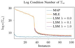
One of the reasons why we recommend using an informative prior for $\boldsymbol{\Sigma}_{\omega}$, is because its MLE estimate is typically numerically unstable. We used the matrix condition number $\kappa(\boldsymbol{\Sigma}_{\omega})$ to measure numerical stability of the Maximum A Posteriori (MAP) and Maximum Likelihood Estimator (MLE) estimates of $\boldsymbol{\Sigma}_{\omega}$. Intuitively, the condition number provides a measure of the sensitivity of an estimated value to small changes in the input data [18]. Therefore, a smaller the condition number means a more numerically stable estimate. Figure 4 shows the change in the condition number for $\boldsymbol{\Sigma}_{\omega}$ in logarithmic scale with respect to the number of training instances for both the MAP and MLE estimates. The condition number for the MAP estimate is depicted in blue, and stabilizes around 6 training instances. On the other hand, the MLE estimate depicted in red requires around 50 training instances to stabilize.

II-C Relation to the Least Squares method to train ProMPs

1:Demonstration dataset containing the joint states and corresponding normalized time stamps $\boldsymbol{Y}=\{\boldsymbol{y}_{nt},z_{nt}\}$ and the prior parameters $k_{0},\boldsymbol{m}_{0},v_{0},\boldsymbol{S}_{0}$

2:The ProMP parameters $\boldsymbol{\mu}_{\omega}$, $\boldsymbol{\Sigma}_{\omega}$, $\boldsymbol{\Sigma}_{y}$

3:Compute matrices $\boldsymbol{\phi}_{nt}=\boldsymbol{\phi}(z_{nt})$ with the basis functions $\boldsymbol{\phi}$

4:Compute $L=\sum_{n=1}^{N}{\tau_{n}}$

5:Set some initial values for $\boldsymbol{\mu}_{\omega}$, $\boldsymbol{\Sigma}_{\omega}$, $\boldsymbol{\Sigma}_{y}$. We use $\boldsymbol{\mu}_{\omega}=\boldsymbol{0}$, $\boldsymbol{\Sigma}_{\omega}=\boldsymbol{I}$ and $\boldsymbol{\Sigma}_{y}=\boldsymbol{I}$.

6:while Not converged do

7:     for  $n\in\{1,\dots,N\}$  do

8:         Compute $\hat{\boldsymbol{w}}_{n}$ with (8)

9:     end for

10:     $\boldsymbol{\mu}_{\omega}^{*}\leftarrow\frac{1}{N}\left(\sum_{n=1}^{N}{\hat{\boldsymbol{w}}_{n}}\right)$

11:     $\boldsymbol{\mu}_{\omega}\leftarrow\frac{1}{N+k_{0}}\left(k_{0}\boldsymbol{m}_{0}+N\boldsymbol{\mu}_{\omega}^{*}\right)$

12:     $\boldsymbol{\Sigma}_{\omega}^{*}\leftarrow\frac{1}{N}{\sum_{n=1}^{N}{\left((\hat{\boldsymbol{w}}_{n}-\boldsymbol{\mu}_{\omega}){(\hat{\boldsymbol{w}}_{n}-\boldsymbol{\mu}_{\omega})}^{\top}\right)}}$

13:     $\boldsymbol{\Sigma}_{\omega}\leftarrow\frac{1}{N+v_{0}+KD+1}\left[\boldsymbol{S}_{0}+N\boldsymbol{\Sigma}_{\omega}^{*}\right]$

14:     $\boldsymbol{\Sigma}_{y}\leftarrow\frac{1}{L}\sum_{n=1}^{N}{\sum_{t=1}^{\tau_{n}}{\left[\boldsymbol{\epsilon}_{nt}{\boldsymbol{\epsilon}_{nt}}^{\top}\right]}}$

15:end while

16:return  $\boldsymbol{\mu}_{\omega}$, $\boldsymbol{\Sigma}_{\omega}$ and $\boldsymbol{\Sigma}_{y}$.

Algorithm 2 EM training algorithm with a Dirac delta approximation for the E-step

An alternative method of training ProMPs was proposed by [16]. We show that the method proposed in [16] is a special case of the EM algorithm presented in this paper for the MLE case, with a single iteration and approximating the Gaussian distributions over the hidden variables $\boldsymbol{\omega}_{n}$ with a Dirac delta distribution on the mean.

The method presented in [16] consists of making point estimates of the hidden variables $\boldsymbol{\omega}_{n}$ with least squares. Subsequently, the mean and covariance of the point estimates are used to estimate the ProMP parameters. The point estimates of $\boldsymbol{\omega}_{n}$ are computed for every trajectory using

$$\boldsymbol{\omega}_{n}=({\boldsymbol{\Phi}_{n}}^{\top}\boldsymbol{\Phi_{n}}+\lambda\boldsymbol{I})^{-1}{\boldsymbol{\Phi}_{n}}^{\top}\boldsymbol{y}_{n},$$ (5)

where $\boldsymbol{\Phi}_{n}$ and $\boldsymbol{y}_{n}$ are the vertical concatenation of the matrices $\boldsymbol{\Phi}_{nt}$ and vectors $\boldsymbol{y}_{nt}$ respectively, and $\lambda$ is a ridge regression parameter that can be set to zero unless numerical problems arise. Subsequently, the ProMP parameters can be estimated using the MLE estimates for Gaussian distributions

$$\boldsymbol{\mu}_{\omega}^{*} =\frac{1}{N}\sum\nolimits_{n=0}^{N}{\boldsymbol{\omega}_{n}},$$ (6)

$$\boldsymbol{\Sigma}_{\omega}^{*} =\frac{1}{N}{\sum\nolimits_{n=0}^{N}{(\boldsymbol{\omega}_{n}-\boldsymbol{\mu}_{\omega}){(\boldsymbol{\omega}_{n}-\boldsymbol{\mu}_{\omega})}^{\top}}.}$$ (7)

Figure 4 shows the numerical stability of the matrix $\boldsymbol{\Sigma}_{\omega}$ of equations (5) to (7) using multiple values of $\lambda$. Note that this training procedure has the same numerical stability issues that the MLE estimates independently of the value of $\lambda$. The reason is that the numerical problems do not come from the estimation of $\omega$, where $\lambda$ is being used, but from the estimation of the covariance matrix itself on (7). Note also that Figure 4 displays the conditioning number of $\boldsymbol{\Sigma}_{\omega}$ for this method using a minimum of 36 demonstrations. The reason is that using (7) with $N<KD$ would result in a rank deficient matrix $\boldsymbol{\Sigma}_{\omega}$ whose condition number would be $+\infty$.

The discussed numerical issues of training a ProMP using (5) to (7) make the learned model dangerous to use directly for robotic applications. In [16], a small diagonal matrix is added to $\boldsymbol{\Sigma}_{\omega}$ and in addition a artificial noise matrix $\boldsymbol{\Sigma}_{y}^{*}$ needs to be used during conditioning. A very large number of training instances $N>>KD$ would be required to be able to use (5) to (7) without any additional tricks. Using the proposed prior distribution solves the numerical problems in a theoretically sound way, and in the limit of infinite amount of data it converges to the expected estimation procedure using maximum likelihood.

However, the estimation method proposed in Algorithm 1 differs from using (5) to (7) in more than just using a prior distribution. To show the differences and similarities, let us now analyze the EM algorithm presented in this paper if we approximate the E-step with a Dirac delta distribution. Note that using a Dirac delta distribution $\delta(\boldsymbol{\omega}-\hat{\boldsymbol{w}}_{n})$ means making a point estimate $\hat{\boldsymbol{w}}_{n}$ of the hidden variables $\boldsymbol{\omega}_{n}$ without any uncertainty. The value of the point estimates $\hat{\boldsymbol{w}}_{n}$ is given by

Algorithm 2 shows the resulting EM algorithm with the discussed approximation for the E-step. The quality of the approximation depends on how much uncertainty is there in the computation of the hidden variables. Let us further assume that we execute one single iteration of Algorithm 2 with initial values $\boldsymbol{\Sigma}_{\omega}=\lambda^{-1}\boldsymbol{I}$, $\boldsymbol{\mu}_{\omega}=0$ and $\boldsymbol{\Sigma}_{y}=\boldsymbol{I}$. It is easy to see that the estimates $\hat{\boldsymbol{w}}_{n}$ would be exactly equivalent to the estimates (5) used by [16]. Note also that Lines 10 and 12 of Algorithm 2 compute also exactly the same estimates of [16] on (6) and (7) for the ProMP parameters in the MLE case.

We can conclude that the training procedure from [16] is equivalent to a single iteration of the approximated training procedure presented in Algorithm 2 on the MLE case with a particular initialization of the ProMP parameters. We have already extensively discussed the advantages of using MAP estimates using the proposed prior distribution. The remaining questions we want to discuss are weather using uncertainty estimates and more than one EM iteration is helpful.

Estimating the uncertainty helps in applications where there is actually high uncertainty in the estimation of the hidden variables $\boldsymbol{\omega}_{n}$ due for example to missing observations or high sensor noise. The answer of how much multiple iterations help depends entirely on the parameter initialization (see Line 5 of Algorithm 2). Note that the only difference between the first iteration and the rest is that in the first iteration we are working entirely on our initial guess of the values of the ProMP parameters. Whereas in subsequent iterations we are using optimized estimates of the ProMP parameters.

For our robot experiments, the sensor noise is on the order of $10^{-3}$ radians and the number of samples per trajectory is between 200 and 500 per degree of freedom. Furthermore, there are no missing observations as we can always read the joint sensor values. With such a low signal to noise ratio and without missing observations the values of the hidden variables $\boldsymbol{\omega}_{n}$ can be estimated very precisely and with low uncertainty. As we expected, we did not observe any difference in the performance in any our our robot experiments using the estimates produced by Algorithms 1 and 2. In fact, the estimated parameters $\boldsymbol{\mu}_{\omega}$ and $\boldsymbol{\Sigma}_{\omega}$ produced by both algorithms are virtually the same. We can conclude that for modeling robot trajectories on a robot setup like ours, using the approximation of the E-step with a Dirac delta distribution does not impact the performance compared to the complete EM estimation.

Figure 5: Log-Likelihood improvement with every iteration of the proposed EM algorithm presented in Algorithm 1 (A1) and the approximated version presented in Algorithm 2 (A5). Both algorithms make initially poor estimates of the hidden variables $\boldsymbol{\omega}_{n}$. However, the proposed algorithm also captures the uncertainty over the estimates of the hidden variables, opposed to the approximated algorithm. As a result, the proposed algorithm continues to successfully improve the likelihood after the first iteration, whereas the approximated algorithm improves only marginally after the first iteration.

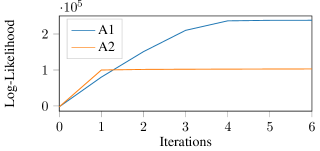
To show an example problem where uncertainty estimates are more important, we decided to run a small additional experiment where we use a ProMPs to model a table tennis ball trajectory. We collected 80 ball trajectories using the robot vision system, there are a few missing observations due to occlusion or errors in the image processing algorithms as well as a higher signal to noise ratio. Subsequently, we trained two models using the exact and approximated training algorithms. Finally, we tested the trained models predicting the ball position at time $t=1.2s$ given the first 160 milliseconds of ball observations. On this experiment, we used $K=8$ basis functions and $D=3$ dimensions. The initial parameters for both algorithms were $\boldsymbol{\Sigma}_{\omega}=\boldsymbol{I}$, $\boldsymbol{\mu}_{\omega}=0$ and $\boldsymbol{\Sigma}_{y}=\boldsymbol{I}$

Figure 5 shows the evaluation of the log likelihood for each iteration of the EM algorithm for both the proposed and the approximated versions. Both algorithms are provided the exact same data and use the exact same parameter initialization. Note that the proposed algorithm outperforms the approximated algorithm in this particular problem. The distance between the ground truth ball position measured by the vision system and the position predicted by the ProMP models trained with Algorithm 1 is around 10 cm, whereas the error of the ProMP trained with Algorithm 2 is around 50 cm.

As a final argument in favour or using Algorithm 1 instead of Algorithm 2, note that we are not gaining anything out of the approximation. The algorithmic complexity is exactly the same in both cases, and estimating the uncertainty does not hurt the learning algorithm even on the cases where it is very low and the approximation seems to be accurate.

III Adaptation of Probabilistic Movement Primitives

(a)

(b)

Figure 6: Task space distributions of the ball and the racket center before and after adapting the ProMP in task space. The distribution of the ball is presented in orange. Figure 6(a) depicts in red the distribution of the center of the racket computed from the ProMP learned from human demonstrations. Subsequently, the ProMP is adapted to hit the ball using Algorithm 3, and the resulting ProMP is depicted in blue in Figure 6(b). Note that the adapted ProMP is similar to the original ProMP learned from human demonstrations, but the probability mass is concentrated in the area that overlaps with the ball trajectory distribution.

Adapting a movement primitive by setting initial positions, desired via points or final positions is a necessary property to generalize to different situations. These desired via points could be specified in joint space or in task space. For example, a table tennis striking movement needs to start in the current joint configuration of the robot and later reach the predicted task space position of the table tennis ball. In this section, we present operators to adapt movement primitives in joint and in task space. In addition, we evaluate the execution time of these operators showing that they can all run in less than one millisecond on a standard computer, satisfying the real time requirements of the applications presented in this paper.

III-A Adapting a ProMP in Joint Space

In the original formulation of ProMPs [10], it was proposed to adapt a ProMP in joint space by conditioning on a desired observation $\boldsymbol{y}_{t}^{*}$ with some noise matrix $\boldsymbol{\Sigma}_{y}^{*}$ that was referred to as the desired accuracy. However, the authors do not provide any intuition on how $\boldsymbol{\Sigma}_{y}^{*}$ should be computed or estimated.

In this paper, we follow the approach presented in previous work [17] to adapt in joint space by conditioning in the distribution over joint trajectories to reach a particular value $\boldsymbol{y}_{t}=\boldsymbol{y}_{t}^{*}$ without any artificial accuracy matrix $\boldsymbol{\Sigma}_{y}^{*}$. The reason why we do not need the artificial noise matrix $\boldsymbol{\Sigma}_{y}^{*}$ opposed to [10] is that we do not suffer from numerical problems inverting $\boldsymbol{\Sigma}_{\omega}$ due to the different training procedure. The conditioned distribution $p(\boldsymbol{\omega}|\boldsymbol{y}_{t}=\boldsymbol{y}_{t}^{*})\propto p(\boldsymbol{y}_{t}=\boldsymbol{y}_{t}^{*}|\boldsymbol{\omega})p(\boldsymbol{\omega})$ can be computed in closed form and is given by

$$p(\boldsymbol{\omega}|\boldsymbol{y}_{t}=\boldsymbol{y}_{t}^{*}) =\mathcal{N}\left({\boldsymbol{\omega}}\,\left|\,{\boldsymbol{m}_{\omega}},{\boldsymbol{S}_{\omega}}\right.\right),$$

$$\boldsymbol{m}_{\omega} =\boldsymbol{S}_{\omega}({\boldsymbol{\phi}_{t}}^{\top}\boldsymbol{\Sigma}_{y}^{-1}\boldsymbol{y}_{t}^{*}+\boldsymbol{\Sigma}_{\omega}^{-1}\boldsymbol{\mu}_{\omega}),$$

$$\boldsymbol{S}_{\omega} =(\boldsymbol{\Sigma}_{\omega}^{-1}+{\boldsymbol{\phi}_{t}}^{\top}\boldsymbol{\Sigma}_{y}^{-1}\boldsymbol{\phi}_{t})^{-1}.$$

There are cases where we do not know the exact value of the desired joint configuration $\boldsymbol{y}_{t}^{*}$, but instead we have a probability distribution $\boldsymbol{y}_{t}^{*}\sim\mathcal{N}\left({\boldsymbol{y}_{t}^{*}}\,\left|\,{\boldsymbol{\mu}_{q}},{\boldsymbol{\Sigma}_{q}}\right.\right)$. For example, in the table tennis task, we need condition the striking movement on the future position of the ball predicted using a Kalman filter. The distribution of the ball is, however, in task space. In Section III-C, we explain how to transform a target task space distribution to a joint space distribution. For the moment, we assume we have a target distribution in joint space, that we can marginalize using

$$p(\boldsymbol{\omega}|\boldsymbol{\mu}_{q},\boldsymbol{\Sigma}_{q})=\int{p(\boldsymbol{\omega}|\boldsymbol{y}_{t}=\boldsymbol{y}_{t}^{*})\mathcal{N}\left({\boldsymbol{y}_{t}^{*}}\,\left|\,{\boldsymbol{\mu}_{q}},{\boldsymbol{\Sigma}_{q}}\right.\right)d{\boldsymbol{y}_{t}^{*}}},$$

which can be computed in closed form obtaining

$$p(\boldsymbol{\omega}|\boldsymbol{\mu}_{q},\boldsymbol{\Sigma}_{q}) =\mathcal{N}\left({\boldsymbol{\omega}}\,\left|\,{\boldsymbol{m}_{\omega}},{\boldsymbol{S}_{\omega}}\right.\right),$$

$$\boldsymbol{m}_{\omega} =\boldsymbol{S}_{\omega}({\boldsymbol{\phi}_{t}}^{\top}\boldsymbol{\Sigma}_{y}^{-1}\boldsymbol{\mu}_{q}+\boldsymbol{\Sigma}_{\omega}^{-1}\boldsymbol{\mu}_{\omega}),$$ (9)

$$\boldsymbol{S}_{\omega} =\boldsymbol{T}_{\omega}+\boldsymbol{T}_{\omega}{\boldsymbol{\phi}_{t}}^{\top}\boldsymbol{\Sigma}_{y}^{-1}\boldsymbol{\Sigma}_{q}\boldsymbol{\Sigma}_{y}^{-1}\boldsymbol{\phi}_{t}\boldsymbol{T}_{\omega},$$ (10)

with $\boldsymbol{T}_{\omega}=(\boldsymbol{\Sigma}_{\omega}^{-1}+{\boldsymbol{\phi}_{t}}^{\top}\boldsymbol{\Sigma}_{y}^{-1}\boldsymbol{\phi}_{t})^{-1}$. The ProMPs can also be adapted with desired velocities or accelerations using the same method, replacing the basis function matrices $\boldsymbol{\phi}_{t}$ by their respective time derivatives $\dot{\boldsymbol{\phi}_{t}}$ and $\ddot{\boldsymbol{\phi}_{t}}$.

The run time complexity for both adaptation operators is bounded by $O(K^{3}D^{3})$. In our robot experiments we used a model with $KD=35$, obtaining an average execution time of 0.044 ms. In the experimental section, we provide running times for different model sizes.

The methods presented here to condition in a ProMP on a particular joint configuration $\boldsymbol{y}_{t}^{*}$ and desired joint distribution were already introduced in previous work [17]. The comparison with the adaptation operator presented in [10] and the analysis of their execution time is new to this paper.

III-B Probability Distribution of a ProMP in Task Space

We compute a probability distribution in task space from a ProMP learned in joint space making use of the geometry of the robot. We assume that we have access to a deterministic function $\boldsymbol{x}_{t}=\boldsymbol{f}(\boldsymbol{y}_{t})$ called the forward kinematics function that returns the position in task space $\boldsymbol{x}_{t}$ of a point of interest like the end effector of the robot given the joint state configuration $\boldsymbol{y}_{t}$. The deterministic forward kinematics function $\boldsymbol{f}$, can be expressed in our probabilistic framework using

$$p(\boldsymbol{x}_{t}|\boldsymbol{y}_{t})=\delta(\boldsymbol{x}_{t}-\boldsymbol{f}(\boldsymbol{y}_{t})),$$

where $\delta$ is the Dirac delta function. The task space distribution can be computed from the ProMP parameters learned in joint space using

$$p(\boldsymbol{x}_{t}|\boldsymbol{\theta}_{\omega})=\int{p(\boldsymbol{y}_{t}|\boldsymbol{\theta}_{\omega})p(\boldsymbol{x}_{t}|\boldsymbol{y}_{t})d\boldsymbol{y}_{t}}.$$

The distribution $p(\boldsymbol{x}_{t}|\boldsymbol{\theta}_{\omega})$ can not be computed in closed form for a non-linear forward kinematics function. We compute an approximated distribution $p(\boldsymbol{x}_{t}|\boldsymbol{\theta}_{\omega})$ making a linear Taylor expansion of the forward kinematics function around the ProMP mean, obtaining

$$p(\boldsymbol{x}_{t}|\boldsymbol{\theta}_{\omega})=\mathcal{N}\left({\boldsymbol{x}_{t}}\,\left|\,{\boldsymbol{f}(\boldsymbol{\Phi}_{t}\boldsymbol{\mu}_{\omega})},{\boldsymbol{J}_{t}\boldsymbol{\Sigma}_{\omega}{\boldsymbol{J}_{t}}^{\top}}\right.\right),$$ (11)

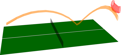
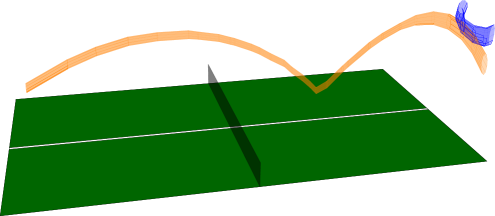
where $\boldsymbol{J}_{t}=\boldsymbol{J}(\boldsymbol{\Phi}_{t}\boldsymbol{\mu}_{\omega})$ is the Jacobian of the forward kinematics function [19] evaluated at $\boldsymbol{y}_{t}=\boldsymbol{\Phi}_{t}\boldsymbol{\mu}_{\omega}$. Figure 6(a) shows the task space distribution of a ProMP learned from demonstrations to strike a table tennis ball as well as some particular ball trajectory distribution. The distribution of the center racket is depicted in red and the distribution of the predicted ball trajectory is depicted in orange.

III-C Adapting ProMPs in Task Space

For many applications, it is more natural to define goals in task space. For instance, in robot table tennis the movement primitive should be adapted such that the position of the racket matches the predicted position of the ball. In this section, we present our approach to condition a ProMP learned in joint space to have a desired task space distribution. The approach we present in this section was also introduced in previous work [17]. However, in this paper we evaluate it more thoroughly on a coffee preparation task with clear training and validation set to assess for generalization.

We denote the desired task space state at time $t$ by the random variable $\boldsymbol{x}_{t}$, with probability distribution given by

$$p(\boldsymbol{x}_{t}|\boldsymbol{\theta}_{x})=\mathcal{N}\left({\boldsymbol{x}_{t}}\,\left|\,{\boldsymbol{\mu}_{x}},{\boldsymbol{\Sigma}_{x}}\right.\right),$$

where the parameters $\boldsymbol{\theta}_{x}=\{\boldsymbol{\mu}_{x},\boldsymbol{\Sigma}_{x}\}$ are user inputs that represent the desired task space configuration and its uncertainty respectively. For the table tennis task, we use a Kalman filter as ball trajectory model. The Kalman filter provides an estimate for the mean ball position $\boldsymbol{\mu}_{x}$ and its uncertainty $\boldsymbol{\Sigma}_{x}$.

Given a desired end effector position $\boldsymbol{x}_{t}$ and a ProMP with parameters $\boldsymbol{\theta}_{\omega}=\{\boldsymbol{\mu}_{\omega},\boldsymbol{\Sigma}_{\omega}\}$, a probability distribution for the joint configuration can be computed by

$$p(\boldsymbol{y}_{t}|\boldsymbol{x}_{t},\boldsymbol{\theta}_{\omega})\propto p(\boldsymbol{x}_{t}|\boldsymbol{y}_{t})p(\boldsymbol{y}_{t}|\boldsymbol{\theta}_{\omega}),$$ (12)

where $p(\boldsymbol{x}_{t}|\boldsymbol{y}_{t})$ is given by (III-B) and $p(\boldsymbol{y}_{t}|\boldsymbol{\theta}_{\omega})$ is the joint space distribution given by the ProMP.

The distribution $p(\boldsymbol{y}_{t}|\boldsymbol{x}_{t},\boldsymbol{\theta}_{\omega})$ represents a compromise between staying close to the demonstrated trajectories and achieving the desired racket configuration. Thus, for a robot arm with redundant degrees of freedom, where multiple joint space configurations can achieve the desired racket configuration, the presented approach will prefer joint solutions that are closer to the demonstrated behavior.

To achieve the desired task space distribution $p(\boldsymbol{x}_{t}|\boldsymbol{\theta}_{x})$ instead of a particular value $\boldsymbol{x}_{t}$, we marginalize out $\boldsymbol{x}_{t}$ from (12) obtaining

$$\begin{split}p(\boldsymbol{y}_{t}|\boldsymbol{\theta}_{x},\boldsymbol{\theta}_{\omega})&=\int{p(\boldsymbol{y}_{t}|\boldsymbol{x}_{t},\boldsymbol{\theta}_{\omega})p(\boldsymbol{x}_{t}|\boldsymbol{\theta}_{x})d{\boldsymbol{x}_{t}}}\\ &\propto p(\boldsymbol{y}_{t}|\boldsymbol{\theta}_{\omega})\int{p(\boldsymbol{x}_{t}|\boldsymbol{\theta}_{x})p(\boldsymbol{x}_{t}|\boldsymbol{y}_{t})d{\boldsymbol{x}_{t}}}.\end{split}$$ (13)

Note that $p(\boldsymbol{y}_{t}|\boldsymbol{\theta}_{x},\boldsymbol{\theta}_{\omega})$ is a distribution in joint space that again compromises between staying close to the demonstrated behavior and achieving the desired task space distribution. The integral in (13), required to compute the normalization constant of $p(\boldsymbol{y}_{t}|\boldsymbol{\theta}_{x},\boldsymbol{\theta}_{\omega})$, is intractable. We used Laplace Approximation [20] to compute a Gaussian approximation for $p(\boldsymbol{y}_{t}|\boldsymbol{\theta}_{x},\boldsymbol{\theta}_{\omega})$. With a Gaussian distribution for $p(\boldsymbol{y}_{t}|\boldsymbol{\theta}_{x},\boldsymbol{\theta}_{\omega})$, the operator to adapt ProMPs in joint space discussed in Section III can be used to obtain a new adapted ProMP.

1:Parameters of desired task space distribution $\boldsymbol{\theta}_{x}=[\boldsymbol{\mu}_{x},\boldsymbol{\Sigma}_{x}]$ and ProMP to adapt $\boldsymbol{\theta}_{\omega}=[\boldsymbol{\mu}_{\omega},\boldsymbol{\Sigma}_{\omega}]$.

2:A new ProMP modulated to strike the ball

3:$\boldsymbol{\mu}_{q}\leftarrow\operatorname*{arg\,max}_{\boldsymbol{y}_{t}}{\left(\log{p(\boldsymbol{y}_{t}|\boldsymbol{\theta}_{x},\boldsymbol{\theta}_{\omega})}\right)}$

4:Compute $\boldsymbol{\Lambda}_{q}$ as the second derivative of $\log{p(\boldsymbol{y}_{t}|\boldsymbol{\theta}_{x},\boldsymbol{\theta}_{\omega})}$ with respect to $\boldsymbol{y}_{t}$ evaluated at $\boldsymbol{y}_{t}=\boldsymbol{\mu}_{q}$

5:$\boldsymbol{\Sigma}_{q}\leftarrow\boldsymbol{\Lambda}_{q}^{-1}$

6:Compute $\boldsymbol{m}_{\omega}$ and $\boldsymbol{S}_{\omega}$ with (9) and (10)

7:return new ProMP with $\boldsymbol{\mu}_{\omega}=\boldsymbol{m}_{\omega}$ and $\boldsymbol{\Sigma}_{\omega}=\boldsymbol{S}_{\omega}$

Algorithm 3 Algorithm to adapt a ProMP in task space using Laplace Approximation

Algorithm 3 describes the procedure to adapt a ProMP in task space using Laplace Approximation. The mean $\boldsymbol{\mu}_{q}$ and covariance $\boldsymbol{\Sigma}_{q}$ of the approximated joint space distribution are computed in Lines 3 and 5 respectively. The presented operator for task space conditioning consists of a non linear optimization to compute $p(\boldsymbol{y}_{t}|\boldsymbol{\theta}_{x},\boldsymbol{\theta}_{\omega})$ followed by a use of the joint space conditioning operator. As a result, the task space conditioning operator is necessarily slower than the joint space conditioning operator. In Section III-D, we show that the execution time of the presented operator is nonetheless reliably below 3 milliseconds for ProMP sizes up to $KD=350$, satisfying the real time requirements of our robot applications by a large margin.

Figure 6 depicts the task space distribution of a ProMP learned from forehand strike demonstrations before 6(a) and after 6(b) adapting it to hit a ball trajectory seen at test time. Note that the adapted ProMP has the probability mass concentrated in the region that overlaps with the ball trajectory distribution.

III-D Execution Time of the Presented Operators

$KD$	Joint Space [ms]	Task Space [ms]
35	$0.0448\pm 0.0164$	$0.7212\pm 0.2920$
70	$0.0642\pm 0.0104$	$0.8328\pm 0.5484$
140	$0.1880\pm 0.0245$	$1.0764\pm 0.3179$
210	$0.5294\pm 0.5879$	$1.4291\pm 0.2423$
280	$0.8686\pm 0.7944$	$1.9267\pm 0.3822$
350	$1.2095\pm 0.4829$	$2.3173\pm 0.3135$

TABLE I: Average execution time of joint and task space conditioning operators in milliseconds for ProMPs of different sizes. The task space operator uses internally the joint space operator, as a result is has a higher execution time. The size of a ProMP is given by the product between the number of degrees of freedom $D$ and the number of kernels per degree of freedom $K$. The table presents the mean and standard deviation of the running times for each operator in milliseconds. For robot table tennis, all these operators need to be executed after the ball trajectory is predicted using ball observations and a ball model. In consequence, it is crucial to be able to apply these operators fast enough to successfully hit the already flying ball.

Many use cases for the operators presented in this paper to adapt the movement primitives will have real time execution requirements. If we want to adapt a movement primitive with respect to sensor values measured at time $t_{1}$ and subsequently execute the movement primitive in the robot at time $t_{2}$, the total execution time for the operator cannot exceed $t_{2}-t_{1}$.

For example, to make sure that the executed movement primitive starts on the current robot joint state, we use the joint conditioning operator on the measured joint state just before starting the execution of the movement primitive. For our robot experiments, we used a control loop of 500 Hertz. Therefore, we have a real time constrain of 2 ms to read the sensor value for the joint state, condition the ProMP to start at the measured value and send the required motor commands.

Table I show the average execution time and standard deviation in milliseconds for the operators presented in this paper. Each operator is executed 1000 times for each of the different sizes of ProMPs in a Lenovo Thinkpad X2 Carbon laptop with a processor Intel Core i7-6500U 2.50GHz and 8 GB of RAM. We report the size as the product of the degrees of freedom $D$ and the number of basis functions per degree of freedom $K$.

On our robot experiment we used a ProMP with size $K=5$ and $D=7$, that corresponds to the smallest entry in Table I. However, note that even on a ProMP with $KD=350$ we can meet the real time requirements to play robot table tennis. The operator to condition in joint space can be reliably run under the 2 milliseconds required for our control loop of 500 Hertz. The vision system we use in this paper produces 60 ball observations per second. Therefore, we can potentially correct the ProMP trajectory to changes in the ball trajectory after every ball observation with a running time below 16 milliseconds. Note that our task space conditioning operator runs reliably under 3 milliseconds, satisfying the real time requirements by a large margin.

IV Experiments and Results

Figure 7: Convergence of the ProMP parameters as a function of the number of training instances in an adversarial scenario. The convergence of different sets of parameters is depicted with different colors. The set of parameters corresponding to the mean behavior, variability of the movement, and correlation between joints are depicted in red, blue and green respectively.

We evaluate the presented methods with synthetic data and with a real robot experiments for table tennis and assisting coffee brewing. For the robot experiments we used Barrett WAM arm with seven degrees of freedom capable of high speed motion. The robot control computer uses a 500 Hz control loop, receiving joint angle measures and output motor commands every 2 ms. To track the position of objects of interest like the table tennis ball and the coffee machine, we used four Prosilica Gigabit cameras and the vision system described in [21]. This vision system tracks the position of a table tennis ball with an approximate frequency of 60 Hz, we attached a table tennis ball to the coffee machine for the coffee brewing experiments.

On all our robot experiments we used five basis functions per degree of freedom. Fifth [13] and third [22] order polynomials have been previously used successfully for robot table tennis approaches. Note that the same results should be achievable with a ProMP with six or four polynomial basis functions respectively taking into account the constant term. On the other hand, radial basis functions (RBFs) have been typically used with ProMPs [10] for other robot applications. We tried different combinations of RBFs and polynomial basis functions, obtaining the best results using three RBFs and a first order polynomial, for a total of five basis functions.

IV-A Parameter Convergence on Synthetic Data

The purpose of the experiment with synthetic data, is to evaluate how accurate are the estimates of the ProMP parameters as a function of the number of training instances $n$ when the assumptions we made for the prior distribution are incorrect. We generate synthetic data from a reference ProMP that displays a strong correlation between different degrees of freedom, opposing the proposed prior assumptions. Subsequently, we test if the proposed learning procedure converges to the expected parameters and how many training examples are necessary for convergence.

Figure 8: The robot executing the coffee task. First, the robot moves towards the top of the coffee grinder to pour fresh beans into it. Subsequently, the robot moves towards the bottom of the grinder to pick the grounds. Finally, the robot deposits the coffee grounds in the brewing chamber of the coffee machine.

On this synthetic data experiment there is no notion of training or test sets. We simply generate $n$ sample trajectories from a reference ProMP with known parameters $\boldsymbol{\mu}_{\omega}$ and $\boldsymbol{\Sigma}_{\omega}$. Subsequently, we train a new ProMP with the sampled trajectories obtaining a new set of parameters $\hat{\boldsymbol{\mu}}_{\omega}^{n}$ and $\hat{\boldsymbol{\Sigma}}_{\omega}^{n}$ and compare how close they are to the reference parameters $\boldsymbol{\mu}_{\omega}$ and $\boldsymbol{\Sigma}_{\omega}$ using the Frobenius norm. In this experiment we used five basis functions $K=5$ and four degrees of freedom $D=4$. To ensure a high correlation, we set the parameters of the base ProMP such that the last two degrees of freedom are the addition and subtraction of the first two degrees of freedom respectively.

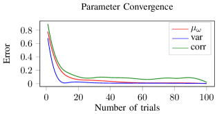
Figure 7 show the average parameter estimation error with respect to the number of training instances $n$ for different set of parameters. The error over the parameters $\boldsymbol{\mu}_{\omega}$ that represent the mean behavior is depicted in red. The error over the parameters $\boldsymbol{\Sigma}_{\omega}$ are divided in the block diagonal terms that represent the captured variability of the movement (depicted in blue) and the rest of the parameters that represent the captured joint correlations (depicted in green). The error of the different set of parameters is normalized between zero and one to facilitate comparison, and the error curves are smoothed out using splines to facilitate visualization of convergence.

Note that the learning algorithm converges to the true value as expected. However, more training examples are required to converge to the correlation parameters because the prior is favouring joint independence in a high joint correlation scenario. The effect of the proposed prior is to prefer independence between the joints in absence of strong evidence of correlation.

The results from this experiment may suggest that the presented probabilistic framework require large amounts of data samples to learn a movement primitive. In contrast, we show we can learn a coffee-pouring and a table-tennis experiment that the proposed approach, using only two and eight training examples respectively. There are two main explanations why we can converge with fewer training instances to the target performance on different tasks. First, the prior distribution assumptions may be more accurate in some real world tasks than in the adversarial example chosen in this section. Second, we can not compare convergence in parameter space to convergence in the performance of a particular task. The reason is that there might be multiple different parameter values with a similar task performance.

IV-B Assisting Coffee Brewing

Figure 9: Training and validation set pattern for the position of the coffee machine, designed to evaluate the generalization on a target area. The training pattern was selected with Lloyd’s algorithm to cover the target area evenly, and is depicted with green circles. The evaluation pattern is depicted in red, and was selected to be far from the training points while covering evenly the target area. The numbers in the green and red circles represent the order used for training and validation positions for the coffee machine respectively.

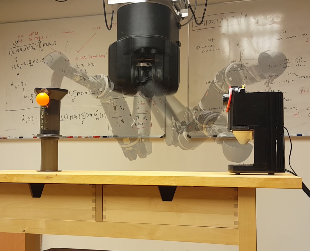
A coffee preparation task was one of the tasks used to evaluate the proposed methods. We use an inexpensive coffee grinder and an Aeropress as a brewing method. Figure 8 depicts the robot executing the steps required to prepare a cup of coffee. First, the robot needs to move to the top of the grinder and pour fresh coffee beans. Subsequently, the robot moves to place the spoon under the grinder funnel to pick the coffee grounds. Finally, the robot pours the coffee grounds into the brewing chamber.

The coffee task requires sequencing movement primitives to pour coffee beans of grounds in different locations and picking the grounds from the grinder. At the same time, the robot should avoid hitting the grinder, coffee machine or the table to prevent damaging the robot, the coffee machines or spilling the coffee. Therefore, this task allows us to test the ability of the proposed framework to divide a complex task into multiple simpler primitives as well as learning from the teacher the right set of movements that avoid hitting external objects.

Additionally, the movement primitives to pour or pick coffee should be adapted to the position of the coffee machine or the grinder in order to succeed. The position of these objects is obtained from the vision system in task space, providing an opportunity to test the operator to adapt movement primitives in task space. The operator to condition movement primitives in joint space is also used to start the executed movement primitive at the robot current joint position.

For the coffee task we want to test how well the proposed approach adapts to changes in the position of the grinder or the coffee machine, whereas for the table tennis task the goal is to determine how well it adapts to changes in the ball trajectory. Note that the position of the grinder and coffee machine in different experiment trials is easy to control with relatively good precision, while controlling the table tennis ball trajectory between different experiment trials is virtually impossible. As a result, we decided to invest more effort in the experiment design to test the generalization ability of a single movement primitive in the coffee task.

1:Training set positions $\{T_{1},\dots,T_{10}\}$ and validation set positions $\{V_{1},\dots,V_{10}\}$ from Figure 9.

2:Training set performance $P^{t}_{n}$ and evaluation set performance $P^{v}_{n}$ with $n$ training samples for $n\in\{1,\dots,10\}$.

3:for  $n\in\{1,\dots,10\}$  do

4:     $\operatorname{train}(\{T_{1},\dots,T_{n}\})$

5:     $P^{t}_{n}\leftarrow\operatorname{evaluate}(\{T_{1},\dots,T_{n}\})$

6:     $P^{v}_{n}\leftarrow\operatorname{evaluate}(\{V_{1},\dots,V_{10}\})$

7:end for

Algorithm 4 Procedure to test the generalization performance of a single ProMP on a pouring coffee experiment

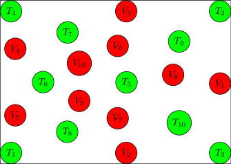
To test the generalization ability of a single movement primitive we focused on the movement that pours the coffee grounds in the coffee machine. We generated a pattern with training and evaluation positions for the coffee machine with a rectangular shape of 42cm x 59.4cm. This size corresponds exactly to an A2 format paper size that was printed for the experiments. To select a set of positions that covers evenly the training area we used Lloyd’s algorithm [23]. For the evaluation set we used an algorithm that selected a set of points in the rectangle that maximized the distance to the training set. Figure 9 shows a resized version of the resulting format for the training and the validation positions for the coffee machine as green and red circles respectively. The numbers on the circles represent the order of the events that should be used in the experiment, and we used them to test the performance on the training and validation sets as a function of the training data. In this experiment we evaluated the success rate of pouring coffee in the machine with a number of training instances varying from 1 to 10 training samples.

The procedure to train and evaluate the performance is explained with detail as a pseudo-code in Algorithm 4. In this pseudo-code the $\operatorname{train}(\cdot)$ function consists on the human training the robot to pour coffee grounds on the coffee machine on the positions passed as argument, and the $\operatorname{evaluate}(\cdot)$ function consists on the robot attempting to pour coffee on the specified positions and evaluating the success rate. For example, to evaluate the validation set performance with two training examples, we would train the robot to pour coffee on positions $\{T_{1},T_{2}\}$ and subsequently evaluate the pouring performance in positions $\{V_{1},\dots,V_{10}\}$.

We used coffee beans instead of coffee grounds on the pouring experiments to simplify the definition of success in a pouring attempt. A trial is considered successful if and only if all the beans end up in the brewing chamber after pouring. No spilling is allowed, a trial is considered failed if one or more beans fall out of the brewing chamber after the pouring movement is executed.

Training Samples	Training	Validation
1	1/1	1/10
{2,…,10}	10/10	10/10

TABLE II: Summary of the results of the generalization performance experiment pouring coffee with a single ProMP. Using only two training samples was enough to generalize to all the target area. With one training sample (T1), the robot succeeded only for the provided training point (T1) and the closest of the validation points (V5), spilling coffee in the rest of the evaluated positions. The obtained results suggest that at least for this task the selected prior is a sensible choice.

Table II summarize the results of the pouring performance measured on this experiment. We expected a curve of generalization performance increasing slowly as a function of the number of training data, but the results obtained showed that after demonstrating the pouring movement only in $T_{1}$ and $T_{2}$ the robot could successfully generalize to all the validation points. With the same two training instances we tried to validate generalization in the points $\{T_{3},\dots,T_{10}\}$ and the robot successfully poured coffee in those positions as well. Note that the results presented in Table II do not mean that the presented approach can generalize to any pouring point given only two demonstrations. If for example, we provide $T_{1}$ and $T_{8}$ as training examples and attempted to validate in the rest of the pouring area, not only the pouring is likely to fail but the resulting planned movement might be dangerous to execute. The ProMPs, as most machine learning methods that assume independently identically distributed data (IID), does not handle extrapolation well. The ProMP framework could be extended using transfer learning techniques [24] to deal better with a non IID scenario, but such an extension is outside the scope of this paper.

With only one training instance of pouring the robot could not generalize well. However, note that the robot managed to pour successfully at the given training position and one of the validation positions. The validation position where the robot poured successfully was $V_{5}$, that is the closest validation point to the given training point $T_{1}$, as can be seen in Figure 9. The distance between $T_{1}$ and $V_{5}$ in the printed pattern is 10.4 cm. We also tried to validate the single training instance example on the points $\{T_{2},\dots,T_{10}\}$, but it failed spilling the coffee every time.

An alternative method to solve the coffee task without learning from human demonstrations would require trajectory planning with collision avoidance in order to succeed. Additionally, common sense knowledge like keeping the spoon pointing up all the time except when the robot is pouring would have to be explicitly programmed. Instead, our approach learns these common sense knowledge and strategies to succeed avoiding collisions with the grinder and brewing chamber from the human demonstrations. In the next section we evaluate our method in a table tennis task. We believe that robot table tennis is significantly harder than the coffee task presented in this section for a number of reasons that we discuss with more detail in the following section. Unfortunately, it is very hard to control precisely the ball trajectory and as a result, we cannot provide detailed generalization performance as with the coffee task. Instead, we will focus on evaluating the hit and return rate performance compared to previous work.

IV-C Robot Table Tennis

Robot table tennis is a highly dynamic task difficult to play for robots and humans. Unlike the coffee task it has strong real time requirements. The timing of the movement is as important as the movement itself to succeed hitting and returning the ball. Furthermore, it is not trivial or obvious which kind on movements would result in success for a given ball trajectory, making this problem especially interesting for learning approaches that can uncover these patterns given a set of successful trial examples.

In this section we evaluate the proposed approach in a robot table tennis setup. In this task we use a table tennis ball gun to throw balls to the robot. Subsequently, we measure weather or not the robot hits the ball and if the ball landed successfully in the opponent’s court according to the table tennis rules.

For all the experiments presented in this section, we collected eight human demonstrations of a particular striking movement to train a ProMP. Unlike the coffee task, the high variability in the results makes it hard to determine the optimal number of training samples to increase the success rate. Informally, we did not notice any significant performance improvements using more than eight demonstrations.

To segment the striking movement from the rest of the demonstrated behavior we used the zero crossing velocity heuristic method. First, we found the point where the racket hit the ball $t_{h}$ by detecting the change in direction of the ball. Subsequently, we found a time interval $(t_{a},t_{b})$ such that $t_{h}\in(t_{a},t_{b})$ and both $t_{a}$ and $t_{b}$ were zero crossing velocity points. We found that this heuristic reliably segments table tennis striking movements if the hitting time $t_{h}$ can be detected accurately. Some times we could not detect the hitting time $t_{h}$ accurately because of vision problems. In such case we simply discarded that trajectory from the training set. We decided to use six as the minimum number of segmented demonstrations in the training set to proceed with the experiments. That is, if more than two demonstrations were discarded by the segmentation heuristic we collected the training data again.

Let us explain in detail how we apply the proposed method to table tennis as well the similarities and differences to previous work presented in [17]. A high level pseudo-code of the table tennis strategy is presented in Algorithm 5. This algorithm receives as input a ProMP already trained to play table tennis using human demonstrations, moves the robot to an initial position and blocks its execution until the vision system produces new ball observations. Subsequently, the obtained ball observations are used to predict the rest of the ball trajectory using a Kalman Filter, the optimal initial time is computed from the ball trajectory using a maximum likelihood approach introduced in previous work [17], and the trained ProMP is conditioned in task space using the operator presented in Section III-B. Before executing the ProMP conditioned to hit the ball, it is conditioned in joint space to start in the current robot joint state.

1:A ProMP promp0 trained for table tennis using human demonstrations.

2:while  running  do

3:     $\text{move\_to\_init\_state}(\text{promp0})$

4:     $\text{wait\_ball\_obs}()$

5:     repeat

6:         $\text{ball\_obs}\leftarrow\text{get\_ball\_obs}()$

7:         $\text{ball\_traj}\leftarrow\text{predict\_ball\_traj}(\text{ball\_obs})$

8:         $t_{0}\leftarrow\text{comp\_optimal\_t0}(\text{ball\_traj})$

9:         $\text{new\_promp}\leftarrow\text{cond\_hit}(\text{promp0},\text{ball\_traj})$

10:     until  $t_{0}\geq\text{current\_time}()$

11:     $\text{new\_promp.cond\_joint\_space}(\text{get\_joint\_state}())$

12:     $\text{execute}(\text{new\_promp})$

13:end while

Algorithm 5 Procedure used on the table tennis experiments

Note that the lines 6 and 9 in Algorithm 5 are in a loop to allow for re-planning. This feature is an important improvement over the previous work presented in [17], because it allows for corrections over the predictions of the ball trajectory produced by the Kalman Filter in line 7. In [17], a set of ball observations of a certain size was obtained and the Kalman Filter was used only once to predict the rest of the ball trajectory. Subsequently, the robot would “close its eyes” and attempt to hit the predicted ball trajectory. In consequence, it was hard to fix a sensible size for the initial set of observations. A small set would not provide enough information to predict accurately the ball trajectory, and a large set could potentially leave a small reaction time to the robot effectively loosing the opportunity to hit the ball. In this paper, we took advantage of the short execution time of the presented operators using re-planning. We simply take any amount of available ball observations to predict the ball trajectory and adapt the ProMP, but we keep doing so while there is still time for corrections.

The starting time of the movement primitive is computed in Line 8 using the operator presented in [17] that maximizes the likelihood of hitting the ball under some assumptions. To compute this likelihood without specifying a hitting time or point, the hitting time was marginalized using some prior distribution. In [17], a uniform distribution was used as prior over the hitting time. We observed that the human teachers usually hit the ball close to the middle of the movement. In consequence, we changed the prior distribution over the hitting time to match the observed teacher behavior. We used a Gaussian distribution given by

$$p_{h}(z)=\mathcal{N}\left({z}\,\left|\,{\mu_{z}=0.5},{\sigma_{z}=0.1}\right.\right)$$

where $z=(t-t_{0})/T$ is the time variable normalized to be between zero and one. As a result, we obtained a substantial improvement on the number of times that the robot manages to successfully return the ball to the opponent’s court, that we will call in the rest of this paper the success rate.

Re-planning	Hit time prior	Hit rate	Success rate
No	Uniform	73.7%	5.2%
No	Gaussian	79.5%	40.9%
Yes	Uniform	93.2%	9.1%
Yes	Gaussian	96.7%	67.7%

TABLE III: Performance improvement for hit and success rate due to re-planning and the prior over the hitting time. The ball gun was fixed to the same settings on these four experiments, and the same ProMP was used in every case trained with Algorithm 1. The goal of these experiments was to test the effect of re-planning and the hitting time prior both independently and combined. Note that re-planning has a significant positive impact mostly over the hitting rate, whereas the prior over the hitting time affects mostly the success rate. The best performance is obtained as expected with a combination of both.

Replanning and the prior over the hitting time are features added to the table tennis strategy on this paper that were not present in [17]. Although these features are unrelated to the main contributions of this paper, we consider important to evaluate the performance improvement due to these features to explain the huge performance gap in comparison to the performance reported in [17]. In addition, the replanning feature is possible only because of the fast execution time of the proposed adaptation operators. Therefore, replanning is an example of how the computational efficiency of the proposed methods can have an impact on the success of a task where accurate prediction models are not available.

Table III presents the results of an experiment to measure the improvement of performance due to re-planning and the hitting time prior both independently and combined. We placed the ball gun in a position that the human teacher found comfortable and collected a set of demonstrations, the ball gun parameters were kept fixed during the rest of the experiment. We trained a ProMP with Algorithm 1 using the collected demonstrations. We use the exact same trained ProMP during this experiment to make sure that the measured improvements are only due to the re-planning and hitting prior features. Note that the change in the prior over the hitting time had a very significant impact on the success rate, increasing it from 5.2% to 40.9% without re-planning and from 9.1% to 67.7% with re-planning. On the other hand, the re-planning feature improved in general about 20% on the hit rate, and the success rate improvement was only substantial in combination with the hitting time prior, improving from 40.9% to 67.7%.

A major difference between this work and [17], is the training algorithm for the movement primitives. In [17], the movement primitives were trained with a maximum likelihood algorithm. In Section II, we discussed how maximum likelihood estimation (MLE) produced unstable estimates of the ProMP parameters opposed to the Maximum A-Posteriori estimates (MAP). To prevent stability problems, the MLE estimates computed in [17] force the matrix $\boldsymbol{\Sigma}_{\omega}$ to be block diagonal. As a result, the computed ProMP considers all the joints independent.

To measure the effect of using the proposed training method opposed to considering all the joints independent with MLE, we tested ProMPs trained with both methods with several ball gun configurations using always the procedure for execution on Algorithm 5 with both re-planning and the prior over the hitting time. We obtained an average success rate of 66.3% and a hit rate of 95.4% for the MAP trained ProMP. For MLE we obtained an average of 47.7% and 79.8% for the hit and success rates respectively.

Figure 10: A human subject moving the robot in gravity compensation mode. Gravity compensation mode was used to obtain the human demonstrations necessary to train the robot.

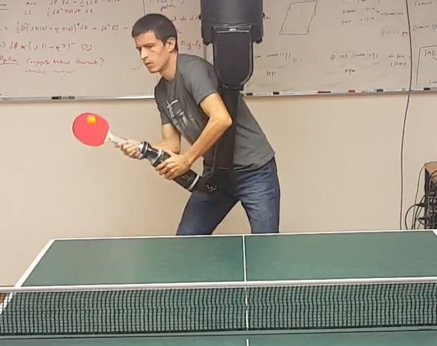
We also compare the performance of our method with a different robot table tennis method based on heuristics [13] called the MoMP method [14]. Figure 10 shows a human subject moving the robot in gravity compensation mode.

(a)

(b)

Figure 11: Histogram of the success and hit rates on table tennis for ProMPs trained with MAP and MLE. We also compare against humans moving the robot in gravity compensation mode and the MoMP method. For the table tennis experiments, repeating the same experiment multiple times will likely produce different hit and success rate performance. In consequence, we decided to present a histogram of the results computed with the bootstrap method representing how likely is it to obtain a particular hit or success rate for different methods.

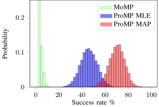
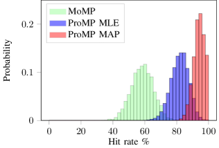
Figure 11 shows an histogram of the success and hit rates obtained in this experiment for both MAP and MLE training, the MoMP method and the human subjects. The histogram was generated with the bootstrap method, generating 5000 random samples of 50 trials from the collected data. The success and hit rates were computed for each of the 5000 samples and recorded in the histogram. We decided to present an histogram of these results instead of just a number to account for the variability of the results natural to the table tennis experiments.

An interval containing 90% of the probability mass of the success rate histogram for the MLE and MAP trained ProMPs would locate the success rate between 34.0% and 58.0% for MLE and between 60.0% and 80.0% for MAP. From these confidence intervals we can conclude that the difference in success rate of learning the joint correlations with the MAP algorithm presented on this paper compared to the MLE algorithm presented in [17] that assumes the joints as independent is significant.

Furthermore, the table tennis procedure presented in Algorithm 5 used for the MAP and MLE trained ProMPs does not include any heuristic or method to successfully return the ball to the opponent’s court. In both cases this behavior has to be learned from the demonstrated data. The fact that the success rate of the MAP trained ProMP is significantly better than the success rate of the MLE trained ProMP that forces $\boldsymbol{\Sigma}_{\omega}$ to be block diagonal, suggests that the joint correlations encode information important to successfully return table tennis balls.

The performance of the presented approach was significantly better than the MoMP method for both hit and success rates in our experiments. The MoMP method is based on several heuristics that would require a great amount of hand tuning to achieve a good success rate for a particular ball gun configuration. As a result, it is very hard to tune this method to generalize well to different ball gun locations and orientations. On the other hand, our method generalizes well to changes on the ball trajectory and can be easily retrained if the ball gun configuration is significantly changed.

V Conclusions and Discussion

This paper introduces new operators to learn and adapt probabilistic movement primitives in joint and in task space. The presented learning algorithm uses a prior distribution to increase the robustness of the estimated parameters. Using the proposed prior distribution over the ProMP parameters is an effective way to improve robustness and learn with few training instances while conserving enough flexibility in the model to learn the dependencies between the joints as more data becomes available.

This paper also presents simple and fast operators to adapt movement primitives in joint and task space, making use of standard methods of probability theory. These operators were evaluated in the coffee task and table tennis task to adapt the learned movement primitive to the coffee machine position and the ball trajectory respectively. The presented operators to adapt movement primitives can be applied to any other robotic applications.

We have compared the table tennis performance of the presented approach with previous work presented in [17]. We tested the performance improvements due to table tennis specific advantages like re-planning and the prior over the hitting time. More importantly, we tested the improvements due to the presented learning algorithm and its ability to learn the joint correlations independently of the table tennis specific improvements. We show that the difference on the learning algorithm alone is enough to obtain a statistically significant improvement.

Unlike previous approaches to robot table tennis, our approach does not model the interaction between the racket and the ball. The reason why the presented method can successfully send balls to the opponent’s side of the table is because the training data used to learn the movement primitive contains mostly successful examples. Thus, the behavior of successfully returning balls is completely learned from data.

A limitation of the presented training method is that it requires manual segmentation of the robot trajectories. Someone needs to specify where every movement primitive starts and ends in the demonstrated behavior. A better approach would be to consider the segmentation as another hidden variable and add it to the proposed EM inference algorithm. The problems of automatic segmentation and clustering should be considered in future work.

Sebastian Gomez-Gonzalez joined the MPI for Intelligent Systems in 2015. He is also affiliated with Technische Universitaet Darmstadt as an external member. His research interests include machine learning, generative models for motion and reinforcement learning. Sebastian received his MSc and BSc degree in computer science from Universidad Tecnologica de Pereira. He obtained the “Best in Education” award for obtaining the best score in Colombia in the standardized test for computer science in 2011.

Gerhard Neumann is a Professor of Robotics & Autonomous Systems in College of Science of Lincoln University. Before coming to Lincoln, he has been an Assistant Professor at the TU Darmstadt. Before that, he was Post-Doc and Group Leader at the Intelligent Autonomous Systems Group (IAS) also in Darmstadt. Gerhard obtained his Ph.D. under the supervision of Prof. Wolfgang Mass at the Graz University of Technology. Gerhard has a strong publication record both in machine learning venues (e.g., NIPS, ICML) and in the robotics community (e.g., ICRA, IROS). He has been active at bringing researchers from both fields together by organizing multiple workshops at the frontier between these two fields, e.g., on reinforcement learning and motor skill acquisition. He served in the senior program committee of some of the most prestigious conferences in artificial intelligence including NIPS and AAAI.

Bernhard Schölkopf ’s scientific interests are in machine learning and causal inference. He has applied his methods to a number of different application areas, ranging from biomedical problems to computational photography and astronomy. Bernhard has researched at AT&T Bell Labs, at GMD FIRST, Berlin, and at Microsoft Research Cambridge, UK, before becoming a Max Planck director in 2001. He is a member of the German Academy of Sciences (Leopoldina), and has received the J.K. Aggarwal Prize of the International Association for Pattern Recognition, the Max Planck Research Award (shared with S. Thrun), the Academy Prize of the Berlin-Brandenburg Academy of Sciences and Humanities, and the Royal Society Milner Award.

Jan Peters is a full professor (W3) for Intelligent Autonomous Systems at the Computer Science Department of the Technische Universitaet Darmstadt and at the same time a senior research scientist and group leader at the Max-Planck Institute for Intelligent Systems, where he heads the interdepartmental Robot Learning Group. Jan Peters has received the Dick Volz Best 2007 US PhD Thesis Runner-Up Award, the Robotics: Science & Systems - Early Career Spotlight, the INNS Young Investigator Award, and the IEEE Robotics & Automation Society’s Early Career Award. Recently, he received an ERC Starting Grant. In 2019, Jan Peters was appointed IEEE Fellow. Jan Peters has studied Computer Science, Electrical, Mechanical and Control Engineering at TU Munich and FernUni Hagen in Germany, at the National University of Singapore (NUS) and the University of Southern California (USC). He has received four Master’s degrees in these disciplines as well as a Computer Science PhD from USC. Jan Peters has performed research in Germany at DLR, TU Munich and the Max Planck Institute for Biological Cybernetics (in addition to the institutions above), in Japan at the Advanced Telecommunication Research Center (ATR), at USC and at both NUS and Siemens Advanced Engineering in Singapore.

References

- [1] J. Nakanishi, J. Morimoto, G. Endo, G. Cheng, S. Schaal, and M. Kawato, “Learning from demonstration and adaptation of biped locomotion,” Robotics and Autonomous Systems, vol. 47, no. 2, pp. 79–91, 2004.
- [2] A. Ude, A. Gams, T. Asfour, and J. Morimoto, “Task-specific generalization of discrete and periodic dynamic movement primitives,” IEEE Transactions on Robotics, vol. 26, no. 5, pp. 800–815, 2010.
- [3] J. Kober, “Learning motor skills: from algorithms to robot experiments,” it-Information Technology, vol. 56, no. 3, pp. 141–146, 2014.
- [4] P. Kormushev, S. Calinon, and D. G. Caldwell, “Robot motor skill coordination with em-based reinforcement learning,” in IEEE International Conference on Intelligent Robots and Systems (IROS). IEEE, 2010, pp. 3232–3237.
- [5] H. Müller and D. Sternad, “Motor learning: changes in the structure of variability in a redundant task,” in Progress in motor control. Springer, 2009, pp. 439–456.
- [6] S. Calinon, F. Guenter, and A. Billard, “On learning, representing, and generalizing a task in a humanoid robot,” IEEE Transactions on Systems, Man, and Cybernetics, Part B (Cybernetics), vol. 37, no. 2, pp. 286–298, 2007.
- [7] A. Billard, S. Calinon, R. Dillmann, and S. Schaal, “Robot programming by demonstration,” in Springer Handbook of Robotics. Springer, 2008, pp. 1371–1394.
- [8] S. Calinon, D. Bruno, and D. G. Caldwell, “A task-parameterized probabilistic model with minimal intervention control,” in IEEE International Conference on Robotics and Automation (ICRA). IEEE, 2014, pp. 3339–3344.
- [9] J. R. Medina, D. Lee, and S. Hirche, “Risk-sensitive optimal feedback control for haptic assistance,” in IEEE International Conference on Robotics and Automation (ICRA). IEEE, 2012, pp. 1025–1031.
- [10] A. Paraschos, C. Daniel, J. Peters, and G. Neumann, “Probabilistic movement primitives,” in Advances in Neural Information Processing Systems, 2013, pp. 2616–2624.
- [11] M. Alvarez, D. Luengo, and N. Lawrence, “Latent force models,” in Artificial Intelligence and Statistics, 2009, pp. 9–16.
- [12] S. Chiappa, J. Kober, and J. R. Peters, “Using bayesian dynamical systems for motion template libraries,” in Advances in Neural Information Processing Systems, 2009, pp. 297–304.
- [13] K. Mülling, J. Kober, and J. Peters, “A biomimetic approach to robot table tennis,” Adaptive Behavior, vol. 19, no. 5, pp. 359–376, 2011.
- [14] K. Mülling, J. Kober, O. Kroemer, and J. Peters, “Learning to select and generalize striking movements in robot table tennis,” The International Journal of Robotics Research, vol. 32, no. 3, pp. 263–279, 2013.
- [15] K. P. Murphy, Machine learning: a probabilistic perspective. MIT Press, 2012.
- [16] A. Paraschos, E. Rueckert, J. Peters, and G. Neumann, “Model-free probabilistic movement primitives for physical interaction,” in IEEE/RSJ International Conference on Intelligent Robots and Systems (IROS). IEEE, 2015, pp. 2860–2866.
- [17] S. Gomez-Gonzalez, G. Neumann, B. Schölkopf, and J. Peters, “Using probabilistic movement primitives for striking movements,” in IEEE-RAS 16th International Conference on Humanoid Robots (Humanoids). IEEE, 2016, pp. 502–508.
- [18] D. A. Belsley, E. Kuh, and R. E. Welsch, Regression diagnostics: Identifying influential data and sources of collinearity. John Wiley & Sons, 2005.
- [19] B. Siciliano, L. Sciavicco, L. Villani, and G. Oriolo, Robotics: Modelling, Planning and Control. Springer Science & Business Media, 2010.
- [20] C. M. Bishop, Pattern recognition and machine learning. Springer, 2006.
- [21] C. H. Lampert and J. Peters, “Real-time detection of colored objects in multiple camera streams with off-the-shelf hardware components,” Journal of Real-Time Image Processing, vol. 7, no. 1, pp. 31–41, 2012.
- [22] O. Koç, G. Maeda, and J. Peters, “Online optimal trajectory generation for robot table tennis,” Robotics and Autonomous Systems, vol. 105, pp. 121 – 137, 2018. [Online]. Available: http://www.sciencedirect.com/science/article/pii/S0921889017306164
- [23] S. Lloyd, “Least squares quantization in pcm,” IEEE Transactions on Information Theory, vol. 28, no. 2, pp. 129–137, 1982.
- [24] S. J. Pan, Q. Yang et al., “A survey on transfer learning,” IEEE Transactions on knowledge and data engineering, vol. 22, no. 10, pp. 1345–1359, 2010.
![[Uncaptioned image]](/html/1808.10648/assets/img/sebastian.jpg) |