Fair Algorithms for Learning in Allocation Problems

Abstract

Settings such as lending and policing can be modeled by a centralized agent allocating a scarce resource (e.g. loans or police officers) amongst several groups, in order to maximize some objective (e.g. loans given that are repaid, or criminals that are apprehended). Often in such problems fairness is also a concern. One natural notion of fairness, based on general principles of equality of opportunity, asks that conditional on an individual being a candidate for the resource in question, the probability of actually receiving it is approximately independent of the individual’s group. For example, in lending this would mean that equally creditworthy individuals in different racial groups have roughly equal chances of receiving a loan. In policing it would mean that two individuals committing the same crime in different districts would have roughly equal chances of being arrested.

In this paper, we formalize this general notion of fairness for allocation problems and investigate its algorithmic consequences. Our main technical results include an efficient learning algorithm that converges to an optimal fair allocation even when the allocator does not know the frequency of candidates (i.e. creditworthy individuals or criminals) in each group. This algorithm operates in a censored feedback model in which only the number of candidates who received the resource in a given allocation can be observed, rather than the true number of candidates in each group. This models the fact that we do not learn the creditworthiness of individuals we do not give loans to and do not learn about crimes committed if the police presence in a district is low.

As an application of our framework and algorithm, we consider the predictive policing problem, in which the resource being allocated to each group is the number of police officers assigned to each district. The learning algorithm is trained on arrest data gathered from its own deployments on previous days, resulting in a potential feedback loop that our algorithm provably overcomes. In this case, the fairness constraint asks that the probability that an individual who has committed a crime is arrested should be independent of the district in which they live. We empirically investigate the performance of our learning algorithm on the Philadelphia Crime Incidents dataset.

1 Introduction

The bulk of the literature on algorithmic fairness has focused on classification and regression problems (see e.g. [14, 17, 19, 16, 10, 26, 8, 25, 27, 20, 7, 6, 4, 3] for a collection of recent work), but fairness concerns also arise naturally in many resource allocation settings. Informally, a resource allocation problem is one in which there is a limited supply of some resource to be distributed across multiple groups with differing needs. Resource allocation problems arise in financial applications (e.g. allocating loans), disaster response (allocating aid), and many other domains — but the primary example that we will focus on in this paper is policing. In the predictive policing problem, the resource to be distributed is police officers, which can be dispatched to different districts. Each district has a different crime distribution, and the goal (absent additional fairness constraints) might be to maximize the number of crimes caught.

Of course, fairness concerns abound in this setting, and recent work (see e.g. [21, 11, 12]) has highlighted the extent to which algorithmic allocation might exacerbate those concerns. For example, Lum and Isaac [21] show that if predictive policing algorithms such as PredPol are trained using past arrest data to predict future crime, then pernicious feedback loops can arise, which misestimate the true crime rates in certain districts, leading to an overallocation of police. Since the communities that Lum and Isaac [21] showed to be overpoliced on a relative basis were primarily poor and minority, this is especially concerning from a fairness perspective. In this work, we study algorithms that both avoid this kind of under-exploration and can incorporate quantitative fairness constraints.

In the predictive policing setting, Ensign et al. [11] implicitly consider an allocation to be fair if police are allocated across districts in direct proportion to the district’s crime rate; generally extended, this definition asks that units of a resource are allocated according to the group’s share of the total candidates for that resource. In our work, we study a different notion of allocative fairness that has a similar motivation to the notion of equality of opportunity proposed by Hardt et al. [14] in classification settings. Informally speaking, it asks that the probability that a candidate for a resource be allocated a resource should be independent of his group. In the predictive policing setting, it asks that conditional on committing a crime, the probability that an individual is apprehended should not depend on the district in which they commit the crime.

To illustrate that our notions of fairness do not depend on whether individuals would prefer to receive or not receive the good, we highlight another setting in which allocative fairness is a natural concern: hiring. Suppose a company wishes to recruit machine learning programmers by advertising on a social media platform. Many such platforms offer the ability to advertise to different demographics of users and charge by the number of times the advertisement is shown to different users (i.e., the number of impressions); a fixed advertising budget can then be viewed as a number of impressions to allocate. Depending on how well the platform can identify programmers within each demographic, the ad may be shown to a higher or lower number of programmers. In this setting, our notion of allocative fairness asks that the probability a programmer is exposed to the hiring ad (and thus, receives the opportunity to apply for a job) does not depend on the programmer’s demographic, and the allocation problem is to maximize the number of programmers reached via the choice of impressions across each demographic, subject to fairness constraints.

1.1 Our Results

To define the extent to which an allocation satisfies our fairness constraint, we must model the specific mechanism by which resources deployed to a particular group reach their intended targets. We study two such discovery models, and we view the explicit framing of this modeling step as one of the contributions of our work; the implications of a fairness constraint depend strongly on the details of the discovery model, and choosing one is an important step in making one’s assumptions transparent.

We study two discovery models which capture two extremes of targeting ability. In the random discovery model, however many units of the resource are allocated to a given group, all individuals within that group are equally likely to be assigned a unit, regardless of whether they are a candidate for the resource or not. In other words, the probability that a candidate receives a resource is equal to the ratio of the number of units of the resource assigned to his group to the size of his group (independent of the number of candidates in the group).

At the other extreme, in the precision discovery model, units of the resource are given only to actual candidates within a group, as long as there is sufficient supply of the resource. In other words, the probability that a candidate receives a resource is equal to the ratio of the number of units of the resource assigned to his group, to the number of candidates within his group.

In the policing setting, these models can be viewed as two extremes of police targeting ability for an intervention like stop-and-frisk. In the random model, police are viewed as stopping people uniformly at random. In the precision model, police have the omniscient ability to identify individuals with contraband, and stop only them. Of course, reality lies somewhere in between.

These different discovery models have different implications for fairness. In the random model, fairness constrains resources to be distributed in amounts proportional to group sizes, regardless of the distribution of candidates, and so is uninteresting from a learning perspective. On the other hand, the precision model yields an interesting fairness-constrained learning problem when the distribution of the number of candidates in each group must be learned via observation, and what counts as a ‘fair’ allocation depends greatly on these distributions.

We study learning in a censored feedback setting: each round, the algorithm can choose a feasible deployment of resources across groups. Then the number of candidates for the current round in each group is drawn from a fixed, but unknown group-dependent distribution (which might be not be independent from the distributions in other groups). The algorithm does not observe the number of candidates present in each group, but only the number of candidates that received the resource. In the policing setting, this corresponds to the algorithm being able to observe the number of arrests, but not the actual number of crimes in each of the districts. Thus, the extent to which the algorithm can learn about the distribution in a particular group is limited by the number of resources it deploys there. The goal of the algorithm is to converge to an optimal fairness-constrained allocation, where here both the objective value of the solution, and the constraints imposed on it, depend on the unknown distributions.

One trivial solution to the learning problem is to sequentially deploy all of one’s resources to each group in turn for a sufficient amount of time to accurately learn the candidate distributions. This would reduce the learning problem to an offline constrained optimization problem, which we show can be efficiently solved by a greedy algorithm. But this algorithm is unreasonable: it has a large exploration phase in which it uses nonsensical deployments, vastly overallocating to some groups and underallocating to others. A much more realistic, natural approach is a greedy-style learning algorithm, which at each round simply uses its current best-guess estimate for the distribution in each group and deploys an optimal fairness-constrained allocation according to these estimates. Unfortunately, as we show, if one makes no assumptions on the underlying distributions, any algorithm that has a guarantee of converging to a fair allocation must behave like the trivial algorithm, deploying vast numbers of resources to each group in turn.

This impossibility result motivates us to consider the learning problem in which the unknown distributions are from a known parametric family. The natural greedy algorithm uses an optimal fair deployment at each round given the maximum likelihood estimates of candidate distributions given its (censored) observations so far; for concreteness, we analyze this algorithm in case of the Poisson distribution, and show that it converges to an optimal fair allocation, but our analysis generalizes for any single-parameter Lipschitz-continuous family of distributions.

Finally, we conduct an empirical evaluation of our algorithm on the Philadelphia Crime Incidents dataset, which records all crimes reported to the Philadelphia Police Department’s INCT system between 2006 and 2016. We verify that the crime distributions in each district are in fact well-approximated by Poisson distributions, and that our algorithm converges quickly to an optimal fair allocation (as measured according to the empirical crime distributions in the dataset). We also systematically evaluate the Price of Fairness, and plot the Pareto curves that trade off the number of crimes caught versus the slack allowed in our fairness constraint, for different sizes of police force, on this dataset. For the random discovery model, we prove worst-case bounds on the Price of Fairness.

1.2 Further Related Work

Our precision discovery model is inspired by and has technical connections to Ganchev et al. [13], which models the dark pool problem from quantitative finance, in which a trader wishes to execute a specified number of trades across a set of exchanges of unknown but independently distributed liquidity. In Ganchev et al. [13], the authors design an optimal allocation algorithm under the censored feedback of the precision model. It is straightforward to map their setting onto ours, but they assume independence between different exchanges, while the candidate distributions in our setting need not be independent. Regardless, we show that their allocation algorithm can be used to compute an optimal allocation (ignoring fairness) even when the independence assumption is relaxed (see Remark 1). Later, Agarwal et al. [1] extend the dark pool problem to an adversarial (rather than distributional) setting. This is quite closely related to the work of Ensign et al. [12] who also consider the precision model (under a different name) in an adversarial predictive policing setting. They provide no-regret algorithms for this setting by reducing the problem to learning in a partial monitoring environment. Since their setting is equivalent to that of Agarwal et al. [1], the algorithms in Agarwal et al. [1] can be directly applied to the problem studied by Ensign et al. [12].

Our desire to study the natural greedy algorithm rather than an algorithm which uses “unreasonable” allocations during an exploration phase is an instance of a general concern about exploration in fairness-related problems [5]. Recent works have studied the performance of greedy algorithms in different settings for this reason [2, 18, 24].

Lastly, the term fair allocation appears in the fair division literature (see e.g. [23] for a survey), but that body of work is technically quite distinct from the problem we study here.

2 Setting

We study an allocator who has $\mathcal{V}$ units of a resource and is tasked with distributing them across a population partitioned into $\mathcal{G}$ groups. Each group is divided into candidates, who are the individuals the allocator would like to receive the resource, and non-candidates, who are the remaining individuals. We let $m_{i}$ denote the total number of individuals in group $i$. The number of candidates $c_{i}$ in group $i$ is a random variable drawn from a fixed but unknown distribution $\mathcal{C}_{i}$ called the (marginal) candidate distribution. We do not make any assumptions about the relationship between the candidate distributions across different groups and in particular these distributions need not be independent. We use $M$ to denote the total size of all groups (i.e., $M=\Sigma_{i\in[\mathcal{G}]}m_{i}$). An allocation $\textbf{v}=(v_{1},\ldots,v_{\mathcal{G}})$ is a partitioning of these $\mathcal{V}$ units, where $v_{i}\in\{0,\ldots,\mathcal{V}\}$ denotes the units of resources allocated to group $i$. Every allocation is bound by a feasibility constraint which requires that $\Sigma_{i\in[\mathcal{G}]}v_{i}\leq\mathcal{V}$.

A discovery model is a (possibly randomized) function $\operatorname{disc}(v_{i},c_{i})$ mapping the number of units $v_{i}$ allocated to group $i$ and the number of candidates $c_{i}$ in group $i$ to the number of candidates discovered in group $i$. In the learning setting, upon fixing an allocation v, the learner will get to observe (a realization of) $\operatorname{disc}(v_{i},c_{i})$ for the realized value of $c_{i}$ for each group $i$. Fixing an allocation v, a discovery model $\operatorname{disc}(\cdot)$ and candidate distributions for all groups $\mathcal{C}=\{\mathcal{C}_{i}:i\in[\mathcal{G}]\}$, we define the total expected number of discovered candidates, $\chi(\textbf{v},\operatorname{disc}(\cdot),\mathcal{C}),$ as

$$\chi\left(\textbf{v},\operatorname{disc}(\cdot),\mathcal{C}\right)=\sum_{i\in[\mathcal{G}]}\mathop{\mathbb{E}}_{c_{i}\sim\mathcal{C}_{i}}\big{[}\operatorname{disc}(v_{i},c_{i})\big{]},$$ (1)

where the expectation is taken over $\mathcal{C}_{i}$ and any randomization in the discovery model $\operatorname{disc}(\cdot)$. When the discovery model and the candidate distributions are fixed, we will simply write $\chi(\textbf{v})$ for brevity. We also use the total expected number of discovered candidates and (expected) utility exchangeably. We refer to an allocation that maximizes the expected number of discovered candidates over all feasible allocations as an optimal allocation and denote it by $\textbf{w}^{*}$.

2.1 Allocative Fairness

For the purposes of this paper, we say that an allocation is fair if it satisfies approximate equality of candidate discovery probability across groups. We call this discovery probability for brevity. This formalizes the intuition that it is unfair if candidates in one group have an inherently higher probability of receiving the resource than candidates in another. Formally, we define our notion of allocative fairness as follows.

Definition 1.

Fix a discovery model $\operatorname{disc}(\cdot)$ and the candidate distributions $\mathcal{C}$. For an allocation v, let

$$f_{i}\left(v_{i},\operatorname{disc}(\cdot),\mathcal{C}_{i}\right)=\mathop{\mathbb{E}}_{c_{i}\sim\mathcal{C}_{i}}\left[\frac{\operatorname{disc}\left(v_{i},c_{i}\right)}{c_{i}}\right],$$

denote the expected probability that a random candidate from group $i$ receives a unit of the resource at allocation v (i.e. the discovery probability in group $i$). Then for any $\alpha\in[0,1]$, v is $\alpha$-fair if

$$\Big{|}f_{i}\left(v_{i},\operatorname{disc}(\cdot),\mathcal{C}_{i}\right)-f_{j}\left(v_{j},\operatorname{disc}(\cdot),\mathcal{C}_{j}\right)\Big{|}\leq\alpha,$$

for all pairs of groups $i$ and $j$.

When it is clear from the context, for brevity, we write $f_{i}({v_{i}})$ for the discovery probability in group $i$. We emphasize that this definition (1) depends crucially on the chosen discovery model, and (2) requires nothing about the treatment of non-candidates. We think of this as a minimal definition of fairness, in that one might want to further constrain the treatment of non-candidates — but we do not consider that extension.

Since discovery probabilities $f_{i}(v_{i})$ and $f_{j}(v_{j})$ are in $\left[0,1\right]$, the absolute value of their difference is in $\left[0,1\right]$. By setting $\alpha=1$ we impose no fairness constraints whatsoever on the allocations, and by setting $\alpha=0$ we require exact fairness.

We refer to an allocation v that maximizes $\chi(\textbf{v})$ subject to $\alpha$-fairness and the feasibility constraint as an optimal $\alpha$-fair allocation and denote it by $\textbf{w}^{\alpha}$. In general, $\chi(\textbf{w}^{\alpha})$ is a non-increasing quantity in $\alpha$, since as $\alpha$ diminishes, the utility maximization problem becomes more constrained.

Remark 1.

We note that both the utility and discovery probabilities can be written solely in terms of the marginal candidate distributions in each of the groups, even when these distributions are not independent. This is because we have (implicitly) assumed that the number of candidates discovered in a group depends only on the number of candidates in the group and the allocation to that group, regardless of the allocations to and the number of candidates in other groups. This assumption together with the linearity of expectation allows us to write the expected utility as in the right hand side of Equation 1.

3 The Precision Discovery Model

We begin by describing the precision model of discovery. Allocating $v_{i}$ units to group $i$ in the precision model results in the discovery of $\operatorname{disc}(c_{i},v_{i})\triangleq\min(c_{i},v_{i})$ candidates. This models the ability to perfectly discover and reach candidates in a group with resources deployed to that group, limited only by the number of deployed resources and the number of candidates present.

The precision model results in censored observations that have a particularly intuitive form. Recall that in general, a learning algorithm at each round gets to choose an allocation v and then observes $\operatorname{disc}(v_{i},c_{i})$ for each group $i$. In the precision model, this results in the following kind of observation: when $v_{i}$ is larger than $c_{i}$, the allocator learns the number of candidates $c_{i}$ present on that day exactly. We refer to this kind of feedback as an uncensored observation. But when $v_{i}$ is smaller than $c_{i}$, all the allocator learns is that the number of candidates is at least $v_{i}$. We refer to this kind of feedback as a censored observation.

The rest of this section is organized as follows. In Sections 3.1 and 3.2 we characterize optimal and optimal fair allocations for the precision model when the candidate distributions are known. In Section 3.3 we focus on learning an optimal fair allocation when these distributions are unknown. We show that any learning algorithm that is guaranteed to find a fair allocation in the worst case over candidate distributions must have the undesirable property that at some point, it must allocate a vast number of its resources to each group individually. To bypass this hurdle, in Section 3.4 we show that when the candidate distributions have a parametric form, a natural greedy algorithm which always uses an optimal fair allocation for the current maximum likelihood estimates of the candidate distributions converges to an optimal fair allocation.

3.1 Optimal Allocation

We first describe how an optimal allocation (absent fairness constraints) can be computed efficiently when the candidate distributions $\mathcal{C}_{i}$ are known. In Ganchev et al. [13], the authors provide an algorithm for computing an optimal allocation when the distributions over the number of shares present in each dark pool are known and the trader wishes to maximize the expected number of traded shares. While they assume that the distributions of shares across different dark pools are independent, our formulation does not require this assumption of independence. Regardless, we can use the same algorithm as in Ganchev et al. [13] to compute an optimal allocation in our setting; this is because, as stated in Remark 1, the utility in both settings can be written solely in terms of the (marginal) candidate distributions even when the candidate distributions are not independent across different groups. Here, we present the high level ideas of their algorithm in the language of our model, and provide full details for completeness in Appendix B.

Let $\mathcal{T}_{i}(c)=\mathrm{Pr}_{c_{i}\sim\mathcal{C}_{i}}[c_{i}\geq c]$ denote the probability that there are at least $c$ candidates in group $i$. We refer to $\mathcal{T}_{i}(c)$ as the tail probability of $\mathcal{C}_{i}$ at $c$. Recall that the value of the cumulative distribution function (CDF) of $\mathcal{C}_{i}$ at $c$ is defined to be

$$\mathcal{F}_{i}(c)=\sum_{c^{\prime}\leq c}\mathrm{Pr}_{c_{i}\sim\mathcal{C}_{i}}\left[c_{i}=c^{\prime}\right].$$

So $\mathcal{T}_{i}(c)$ can be written in terms of CDF values as $\mathcal{T}_{i}(c)=1-\mathcal{F}_{i}(c-1)$.

First, observe that the expected total number of candidates discovered by an allocation in the precision model can be written in terms of the tail probabilities of the candidate distributions i.e.

$$\chi(\textbf{v},\operatorname{disc}(\cdot),\mathcal{C})=\sum_{i\in[\mathcal{G}]}\mathop{\mathbb{E}}_{c_{i}\sim\mathcal{C}_{i}}\left[\min\left(v_{i},c_{i}\right)\right]=\sum_{i\in[\mathcal{G}]}\sum\limits_{c=1}^{v_{i}}\mathcal{T}_{i}(c).$$

Since the objective function is concave (as $\mathcal{T}_{i}(c)$ is a non-increasing function in $c$ for all $i$), a greedy algorithm which iteratively allocates the next unit of the resource to a group in

$$\operatorname*{arg\,max}\limits_{i\in[\mathcal{G}]}\left(\mathcal{T}_{i}\left(v_{i}^{t}+1\right)-\mathcal{T}_{i}\left(v_{i}^{t}\right)\right),$$

where $v_{i}^{t}$ is the current allocation to group $i$ in the $t$^th round achieves an optimal allocation.

3.2 Optimal Fair Allocation

We next show how to compute an optimal $\alpha$-fair allocation in the precision model when the candidate distributions are known and do not need to be learned.

To build intuition for how the algorithm works, imagine that the group $i$ has the highest discovery probability in $\textbf{w}^{\alpha}$, and the allocation $w^{\alpha}_{i}$ to that group is somehow known to the algorithm ahead of time. The constraint of $\alpha$-fairness then implies that the discovery probability for each other group $j$ in $\textbf{w}^{\alpha}$ must satisfy $f_{j}\in[f_{i}-\alpha,f_{i}]$. This in turn implies upper and lower bounds on the feasible allocations $w^{\alpha}_{j}$ to group $j$. The algorithm is then simply a constrained greedy algorithm: subject to these implied constraints, it iteratively allocates units so as to maximize their marginal probability of reaching another candidate. Since the group $i$ maximizing the discovery probability in $\textbf{w}^{\alpha}$ and the corresponding allocation $w^{\alpha}_{i}$ are not known ahead of time, the algorithm simply iterates through each possible choice of $i$.

$\alpha$, $\mathcal{C}$ and $\mathcal{V}$.

An optimal $\alpha$-fair allocation $\textbf{w}^{\alpha}$.

$\textbf{w}^{\alpha}\leftarrow\vec{0}$. $\triangleright$ Initialize the output.

$\chi_{\max}\leftarrow 0$. $\triangleright$ Keep track of the utility of the output.

for $i\in[\mathcal{G}]$ do$\triangleright$ Guess for group with the highest probability of discovery.

     $\textbf{v}\leftarrow\vec{0}$.

     for $v_{i}\in\{0,\ldots\mathcal{V}\}$ do$\triangleright$ Guess for the allocation to that group.

         Set $v_{i}$ in v and compute $f_{i}(v_{i})$.

         $ub_{i}\leftarrow v_{i}$. $\triangleright$ Upper bound on allocation to group $i$.

         $lb_{i}\leftarrow v_{i}$. $\triangleright$ Lower bound on allocation to group $i$.

         for $j\neq i,j\in[\mathcal{G}]$ do $\triangleright$ Upper and lower bounds for other groups.

              Update $lb_{j}$ and $ub_{j}$ using $f_{i}(v_{i})$, $\alpha$ and $\mathcal{C}_{j}$.

              $v_{j}\leftarrow lb_{j}$. $\triangleright$ Assign the lower bound allocation to group $j$.          

         if $\Sigma_{i\in[\mathcal{G}]}v_{i}>\mathcal{V}$ then

              continue. $\triangleright$ Allocation is not feasible.          

         $\mathcal{V}_{r}=\mathcal{V}-\Sigma_{i\in[\mathcal{G}]}v_{i}$

         for $t=1,\ldots,\mathcal{V}_{r}$ do$\triangleright$ Allocate the remaining resources greedily while obeying fairness.

              $j^{*}\in\operatorname*{arg\,max}\limits_{j\in[\mathcal{G}]}\left(\mathcal{T}_{j}(v_{j}+1)-\mathcal{T}_{j}(v_{j})\right)$ s.t. $v_{j}<ub_{j}$.

              $v_{j^{*}}\leftarrow v_{j^{*}}+1$.          

         $\chi(\textbf{v})=\Sigma_{i\in[\mathcal{G}]}\Sigma_{c=1}^{v_{i}}\mathcal{T}_{i}(c)$. $\triangleright$ Compute the utility of v.

         if $\chi(\textbf{v})>\chi_{\max}$ then$\triangleright$ Update the best $\alpha$-fair allocation found so far.

              $\chi_{\max}\leftarrow\chi(\textbf{v}).$

              $\textbf{w}^{\alpha}\leftarrow\textbf{v}$.               

return $\textbf{w}^{\alpha}$.

Algorithm 1 Computing an optimal fair allocation in the precision model

Pseudocode is given in Algorithm 1. We prove that Algorithm 1 returns an optimal $\alpha$-fair allocation in Theorem 1. We defer the proof of Theorem 1 and all the other omitted proofs in the section to Appendix B.

Theorem 1.

Algorithm 1 computes an optimal $\alpha$-fair allocation for the precision model in time $O(\mathcal{G}\mathcal{V}(\mathcal{G}\mathcal{V}+M))$.

3.3 Learning Fair Allocations Generally Requires Brute-Force Exploration

In Sections 3.1 and 3.2 we assumed the candidate distributions were known. When the candidate distributions are unknown, learning algorithms intending to converge to optimal $\alpha$-fair allocations must learn a sufficient amount about the distributions in question to certify the fairness of the allocation they finally output. Because learners must deal with feedback in the censored observation model, this places constraints on how they can proceed. Unfortunately, as we show in this section, if candidate distributions are allowed to be worst-case, this will force a learner to engage in what we call “brute-force exploration” — the iterative deployment of a large fraction of the resources to each subgroup in turn. This is formalized in Theorem 2.

Theorem 2.

Define $m^{*}=\max_{i\in[\mathcal{G}]}m_{i}$ to be the size of the largest group and assume $m_{i}>6$ for all $i$ and $\mathcal{G}\geq 2$. Let $\alpha\in[0,1/(2m^{*}))$, $\delta\in(0,1/2)$, and $\mathcal{A}$ be any learning algorithm for the precision model which runs for a finite number of rounds and outputs an allocation. Suppose that there is some group $i$ for which $\mathcal{A}$ has not allocated at least $m_{i}/2$ units for at least $k\ln(1/\delta)/(\alpha m_{i})$ rounds upon termination, where $k$ is an absolute constant. Then there exists a candidate distribution such that, with probability at least $\delta$, $\mathcal{A}$ outputs an allocation that is not $\alpha$-fair.

Sketch of the Proof.

Let $i$ denote a group in which $\mathcal{A}$ has not allocated at least $m_{i}/2$ units for at least $k\ln(1/\delta)/(\alpha m_{i})$ rounds upon its termination and let v denote an arbitrary allocation. We will design two candidate distributions for group $i$ which have true discovery probabilities that are at least $2\alpha$ apart given $v_{i}$, but which are indistinguishable given the observations of the algorithm with probability at least $\delta$. If the $\mathcal{A}$ cannot distinguish between $\mathcal{C}_{i}$ and $\mathcal{C}_{i}^{\prime}$, it cannot distinguish between $f_{i}$ and $f_{i}^{\prime}$, and thus cannot guarantee whether group $i$’s discovery probability is indeed within $\alpha$ of every other group’s discovery probability.

To design these candidate distributions, consider distributions $\mathcal{C}_{i}$ and $\mathcal{C}_{i}^{\prime}$ which satisfy the following four conditions.

1. $\mathcal{C}_{i}$ and $\mathcal{C}_{i}^{\prime}$ agree on all values less than $m_{i}/2-2$.

2. The total mass of both distributions below $m_{i}/2-2$ is $1-2\alpha m_{i}$.

3. The remaining $2\alpha m_{i}$ mass of $\mathcal{C}_{i}$ is on the value $m_{i}/2-1$.

4. The remaining $2\alpha m_{i}$ mass of $\mathcal{C}_{i}^{\prime}$ is on the value $m_{i}$.

Distinguishing between $\mathcal{C}_{i}$ and $\mathcal{C}^{\prime}_{i}$ requires at least one uncensored observation beyond $m_{i}/2-2$. However, conditioned on allocating at least $m_{i}/2$ units, the probability of observing an uncensored observation is at most $2\alpha m_{i}$. So to distinguish between $\mathcal{C}_{i}$ and $\mathcal{C}_{i}^{\prime}$ with confidence $1-\delta$, and therefore to guarantee an $\alpha$-fair allocation, a learning algorithm must allocate at least $m_{i}/2$ units to group $i$ for $k\ln(1/\delta)/(\alpha m_{i})$ rounds. ∎

Recall that we used $m^{*}$ to denote the size of the largest group. When $m^{*}>2\mathcal{V}$, then Theorem 2 implies that no algorithm can guarantee $\alpha$-fairness for sufficiently small $\alpha$. Moreover, even when $m^{*}\leq 2\mathcal{V}$, Theorem 2 shows that in general, if we want algorithms that have provable guarantees for arbitrary candidate distributions, it is impossible to avoid something akin to brute-force search (recall that there is a trivial algorithm which simply allocates all resources to each group in turn, for sufficiently many rounds to approximately learn the CDF of the candidate distribution, and then solves the offline problem). In the next section, we circumvent this by giving an algorithm with provable guarantees, assuming that the candidate distributions have a known parametric form.

3.4 Poisson Distributions and Convergence of the MLE

In this section, we assume that all the candidate distributions have a particular and known parametric form but that the parameters of the these distributions are not known to the allocator. Concretely, we assume that the candidate distribution for each group is Poisson (denoted by $\mathcal{C}(\lambda)$) and write $\bm{\lambda}^{*}=(\lambda^{*}_{1},\dots,\lambda^{*}_{\mathcal{G}})$ for the true underlying parameters of the candidate distributions; this choice appears justified, at least in the predictive policing application, as the candidate distributions in the Philadelphia Crime Incidents dataset are well-approximated by Poisson distributions (see Section 4 for further discussion). This assumption allows an algorithm to learn the tails of these distributions without needing to rely on brute-force search, thus circumventing the limitation given in Theorem 2. Indeed, we show that (a small variant of) the natural greedy algorithm incorporating these distributional assumptions converges to an optimal fair allocation.

For simplicity, we assume a parametric form on the marginal candidate distribution in each of the groups. We could have equivalently assumed that the candidates across groups are drawn from a multivariate Poisson distribution to highlight the (potential) correlation between candidates distributions. However, since for a given multivariate Poisson distribution the marginal distribution on each group is itself a Poisson distribution [15], we made our parametric assumption directly on these marginal distributions.

At a high level, in each round, our algorithm uses Algorithm 1 to calculate an optimal fair allocation with respect to the current maximum likelihood estimates of the group distributions; then, it uses the new observations it obtains from this allocation to refine these estimates for the next round. This is summarized in Algorithm 2. The algorithm differs from this pure greedy strategy in one respect, to overcome the following subtlety: there is a possibility that Algorithm 1, when operating on a preliminary estimate for the candidate distributions, will suggest sending zero units to some group, even when the optimal allocation for the true distributions sends some units to every group. Such a deployment would result in the algorithm receiving no feedback for the zero-allocated group that round. If this suggestion is followed and a lack of feedback is allowed to persist indefinitely, the algorithm’s parameter estimate for the zero-allocated group will also stop updating — potentially at an incorrect value. In order to avoid this problem and continue making progress in learning, our algorithm chooses another allocation in this case. As we show, any allocation that allocates positive resources to all groups will suffice; in particular, our algorithm makes the natural choice of simply repeating the allocation from the previous round.

$\alpha$, $\mathcal{V}$ and $T$ (total number of rounds).

An allocation $\textbf{v}^{T+1}$ and estimates to parameters $\{\lambda_{i}^{T}\}$.

$\textbf{v}^{1}\leftarrow(\lfloor(\mathcal{V}/\mathcal{G})\rfloor,\ldots,\lfloor(\mathcal{V}/\mathcal{G})\rfloor)$.$\triangleright$ Allocate uniformly.

for rounds $t=1,\dots,T$ do

     if $\exists i\text{ such that }v_{i}^{t}==0$ then$\triangleright$ Check whether every group is allocated a resource.

         $\textbf{v}^{t}\leftarrow\textbf{v}^{t-1}$.      

     Observe $o^{t}_{i}=\min\{v_{i}^{t},c_{i}^{t}\}$ for each group.

     for $i=1,\ldots,\mathcal{G}$ do

         Update history $\textbf{h}_{i}^{t+1}$ with $o^{t}_{i}$ and $v_{i}^{t}$.

         $\hat{\lambda}_{i}^{t}\leftarrow\operatorname*{arg\,max}_{\lambda\in[\lambda_{\min},\lambda_{\max}]}\hat{\mathcal{L}}(\textbf{h}_{i}^{t+1},\lambda)$. $\triangleright$ Solve the maximum likelihood estimation problem.      

     $\textbf{v}^{t+1}\leftarrow\text{Algorithm}~{}\ref{alg:opt-fair-dark-pool}(\alpha,\{\mathcal{C}(\hat{\lambda}_{i}^{t})\},\mathcal{V})$. $\triangleright$ Compute an allocation to be deployed in the next round.

return $\textbf{v}^{T+1}$ and $\{\lambda_{i}^{T}\}$.

Algorithm 2 Learning an optimal fair allocation

Notice that Algorithm 2 chooses an allocation at every round which is fair with respect to its estimates of the parameters of the candidate distributions; hence, asymptotic convergence of its output to an optimal $\alpha$-fair allocation follows directly from the convergence of the estimates to true parameters. However, we seek a stronger, finite sample guarantee, as stated in Theorem 3.

Theorem 3.

Let $\epsilon,\delta>0$. Suppose that the candidate distributions are Poisson distributions with unknown parameters in the vector $\bm{\lambda}^{*}$, where $\bm{\lambda}^{*}$ lies in the known interval $[\lambda_{\min},\lambda_{\max}]^{\mathcal{G}}$. Suppose we run Algorithm 2 for $t>\tilde{\mathcal{O}}(\ln(\mathcal{G}/\delta)/(\eta(\epsilon))^{2})\triangleq T_{\max}$ rounds, where $\eta(\cdot)$ is some distribution specific function to get an allocation $\hat{\textbf{v}}$ and estimated parameters $\hat{\lambda}_{i}$ for all groups $i$. Then with probability at least $1-\delta$

1. For all $i$ in $[\mathcal{G}]$, $|\hat{\lambda}_{i}-\lambda^{*}_{i}|\leq\epsilon$.

2. Let $D=\max_{i\in[\mathcal{G}]}D_{TV}(\mathcal{C}(\lambda^{*}_{i}),\mathcal{C}(\hat{\lambda}_{i}))$ where $D_{TV}$ denotes the total variation distance between two distributions. Then $\hat{\textbf{v}}$

   • is $(\alpha+4D)$-fair.

   • has utility at most $4D\mathcal{G}\mathcal{V}$ smaller than the utility of an optimal $(\alpha-4D)$-fair allocation i.e. $\chi(\hat{\textbf{v}})\geq\chi(\textbf{w}^{\alpha-4D})-4D\mathcal{G}\mathcal{V}$.

Remark 2.

Theorem 3 implies that in the limit, the allocation from Algorithm 2 will converge to an optimal $\alpha$-fair allocation. As $t\to\infty$, $\hat{\lambda}_{i}\overset{p}{\to}\lambda^{*}_{i}$ for all $i$, meaning $D\to 0$ and more importantly, $\hat{\textbf{v}}$ will be $\alpha$-fair and optimal.

The rest of this section is dedicated to the proof of Theorem 3. First, we introduce notation. Since we assumed the candidate distribution for each group is Poisson, the probability mass function (PMF) and the CDF of the candidate distribution $\mathcal{C}_{i}$ for group $i$ can be written as

$$\mathrm{Pr}_{c_{i}\sim\mathcal{C}(\lambda^{*}_{i})}\left[c_{i}=c;\lambda^{*}_{i}\right]=\frac{{\lambda^{*}_{i}}^{c}e^{-\lambda^{*}_{i}}}{c!}\text{ and }F(c;\lambda^{*}_{i})=\mathrm{Pr}_{c_{i}\sim\mathcal{C}(\lambda^{*}_{i})}\left[c_{i}\leq c;\lambda^{*}_{i}\right]=e^{-\lambda^{*}_{i}}\sum_{x=0}^{c}\frac{{\lambda^{*}_{i}}^{x}}{x!}.$$

Given an allocation of $v_{i}$ units of the resource to group $i$ we use $o_{i}$ to denote the (possibly censored) observation received by Algorithm 2. So while the candidates in group $i$ are generated according to $\mathcal{C}(\lambda^{*}_{i})$, the observations of Algorithm 2 follow a censored Poisson distribution which we abbreviate by $\mathcal{C}_{o}(\lambda^{*}_{i},v_{i})$. We can write the PMF of this distribution as

$$\mathrm{Pr}_{o_{i}\sim\mathcal{C}_{o}(\lambda^{*}_{i},v_{i})}[o_{i}=o;\lambda^{*}_{i},v_{i}]=\begin{cases}\frac{{\lambda^{*}_{i}}^{o}e^{-\lambda^{*}_{i}}}{o!},&o<v_{i},\\ 1-F(v_{i}-1;\lambda^{*}_{i}),&o=v_{i},\end{cases}$$

where $F(v_{i}-1;\lambda^{*}_{i})$ is the CDF value of $\mathcal{C}(\lambda^{*}_{i})$ at $v_{i}-1$.

Since Algorithm 2 operates in rounds, we use the superscript $t$ throughout to denote the round. For each round $t$, denote the history of the units allocated to group $i$ and observations received (candidates discovered) in rounds up to $t$ by $h^{t}_{i}=(v_{i}^{1},o^{1}_{i},\ldots,v_{i}^{t-1},o^{t-1}_{i})$. We use $\textbf{h}^{t}=(h^{t}_{1},\dots,h^{t}_{\mathcal{G}})$ to denote the history for all groups. All the probabilities and expectations in this section are over the randomness of the observations drawn from the censored Poisson distributions unless otherwise noted; we suppress related notation for brevity. Finally, an allocation function $\mathcal{A}$ in round $t$ is a mapping from the history of all groups $\textbf{h}^{t}$ to the number of units to be allocated to each group i.e. $\mathcal{A}:\textbf{h}^{t}\rightarrow\textbf{v}^{t}$. For convenience, we use $\mathcal{A}(\textbf{h}^{t})_{i}$ to denote the allocation $v_{i}^{t}$ at round $t$. We are now ready to define the likelihood functions.

Definition 2.

Let $p(v_{i}^{t},o^{t}_{i};\lambda):=\mathrm{Pr}[o^{t}_{i};\lambda,v_{i}^{t}]$ denote the (censored) likelihood of discovering $o^{t}_{i}$ candidates given an allocation $v_{i}^{t}$ to group $i$ assuming the candidate distribution follows $\mathcal{C}(\lambda)$. We write $\ell(v_{i}^{t},o^{t}_{i};\lambda)$ as $\log p(v_{i}^{t},o^{t}_{i};\lambda)$. So, given any history $\textbf{h}^{t}$, the empirical log-likelihood function for group $i$ is

$$\hat{\mathcal{L}}_{i}\left(\textbf{h}^{t},\lambda\right)=\frac{1}{t}\sum_{s=1}^{t}\ell\left(\mathcal{A}(\textbf{h}^{s})_{i},o^{s}_{i};\lambda\right).$$

The expected log-likelihood function given the history of allocations but over the randomness of the candidacy distribution can be written as

$$\mathcal{L}^{*}_{i}\left(\textbf{h}^{t},\lambda\right)=\frac{1}{t}\sum_{s=1}^{t}\mathop{\mathbb{E}}\left[\ell\left(\mathcal{A}(\textbf{h}^{s})_{i},o^{s}_{i};\lambda\right)\right],$$

where the expectation is over the randomness of $o^{s}_{i}$ drawn from $\mathcal{C}_{o}(\lambda^{*},\mathcal{A}(\textbf{h}^{s})_{i})$.

Proof of Theorem 3

To prove Theorem 3, we first show that any sequence of allocations selected by Algorithm 2 will eventually recover the true parameters. There are two conceptual difficulties here: the first is that standard convergence results typically leverage the assumption of independence, which does not hold in this case as Algorithm 2 computes adaptive allocations which depend on the allocations in previous rounds; the second is the censoring of the observations. Despite these difficulties, we give quantifiable rates with which the estimates converge to the true parameters. Next, we show that computing an optimal $\alpha$-fair allocation using the estimated parameters will result in an allocation that is $(\alpha+4D)$-fair with respect to the true candidate distributions where $D$ denotes the maximum total variation distance between the true and estimated Poisson distributions across all groups. Finally, we show that this allocation also achieves a utility that is comparable to the utility of an optimal $(\alpha-4D)$-fair allocation. We note that while Theorem 3 is only stated for Poisson distributions, our results can be generalized to any single parameter Lipschitz-continuous family of distributions (see Remark 3).

Closeness of the Estimated Parameters

Our argument can be stated at a high level as follows: for any group $i$ and any history $\textbf{h}^{t}$, the empirical log-likelihood converges to the expected log-likelihood for any sequence of allocations made by Algorithm 2 as formalized in Lemma 1. We then show in Lemma 2 that the closeness of the empirical and expected log-likelihoods implies that the maximizers of these quantities (corresponding to the estimated and true parameters) will also become close. Since in our analysis we consider the groups separately, we fix a group $i$ throughout the rest of this section and drop the subscript $i$ for convenience.

We start by studying the rate of convergence of the empirical log-likelihood to the expected log-likelihood.

Lemma 1.

With probability at least $1-\delta/\mathcal{G}$, for any $t$ and any $\textbf{h}^{t}$ observed by Algorithm 2

$$\sup_{\lambda\in[\lambda_{min},\lambda_{max}]}\left|\hat{\mathcal{L}}\left(\textbf{h}^{t},\lambda\right)-\mathcal{L}^{*}\left(\textbf{h}^{t},\lambda\right)\right|\leq\mathcal{O}\left(\sqrt{\frac{\ln(t\mathcal{G}/\delta)}{t}}\right).$$

The true and estimated parameters for each group correspond to the maximizers of the expected and empirical log-likelihoods, respectively (see Corollary 1 in Appendix B). We next show that closeness of the empirical and expected log-likelihoods implies that the true and estimated parameters are also close.

Lemma 2.

Let $\hat{\lambda}$ denote the estimate of the Algorithm 2 after $T_{\max}$ rounds. Then with probability at least $1-\delta/\mathcal{G}$, $\ |\hat{\lambda}-\lambda^{*}|<\epsilon$.

Proof.

Since Corollary 1(in Appendix B) gives that $\mathcal{L}(\textbf{h}^{t},\lambda)$ has a unique maximizer at $\lambda^{*}$ and Corollary 3(in Appendix B) gives that there exists some $\eta(\epsilon)$ so that for any $\lambda^{\prime}$ such that $|\mathcal{L}^{*}(\textbf{h}^{t},\lambda^{\prime})-\mathcal{L}^{*}(\textbf{h}^{t},\lambda^{*})|<\eta(\epsilon)$, we must have that $|\lambda^{\prime}-\lambda^{*}|<\epsilon$. We denote $\eta(\epsilon)$ by $\eta$ for brevity. We define the empirical maximizer $\hat{\lambda}$ to be the maximizer of $\hat{\mathcal{L}}(\textbf{h}^{t},\lambda)$ i.e.

$$\hat{\lambda}\in\operatorname*{arg\,max}_{\lambda\in\left[\lambda_{\min},\lambda_{\max}\right]}\hat{\mathcal{L}}\left(\textbf{h}^{t},\lambda\right).$$ (2)

Applying Lemma 1 implies that for any $\textbf{h}^{t}$ with $t>T_{\max}$ and $\lambda^{\prime}\in[\lambda_{\min},\lambda_{\max}]$, with probability at least $1-\delta/\mathcal{G}$,

$$\left|\hat{\mathcal{L}}(\textbf{h}^{t},\lambda^{\prime})-\mathcal{L}^{*}(\textbf{h}^{t},\lambda^{\prime})\right|<\frac{\eta}{2}.$$

In particular, we must have that

$$\left|\hat{\mathcal{L}}\left(\textbf{h}^{t},\lambda^{*}\right)-\mathcal{L}^{*}\left(\textbf{h}^{t},\lambda^{*}\right)\right|<\frac{\eta}{2}\qquad\text{and}\qquad\left|\hat{\mathcal{L}}\left(\textbf{h}^{t},\hat{\lambda}\right)-\mathcal{L}^{*}\left(\textbf{h}^{t},\hat{\lambda}\right)\right|<\frac{\eta}{2}.$$ (3)

Since $\hat{\lambda}$ is a maximizer of Equation 2, we have that

$$\hat{\mathcal{L}}\left(\textbf{h}^{t},\hat{\lambda}\right)\geq\hat{\mathcal{L}}\left(\textbf{h}^{t},\lambda^{*}\right)\geq\mathcal{L}^{*}\left(\textbf{h}^{t},\lambda^{*}\right)-\frac{\eta}{2},$$

where the last inequality is by Equation 3. This implies that

$$\mathcal{L}^{*}\left(\textbf{h}^{t},\hat{\lambda}\right)>\hat{\mathcal{L}}\left(\textbf{h}^{t},\hat{\lambda}\right)-\frac{\eta}{2}>\mathcal{L}^{*}\left(\textbf{h}^{t},\lambda^{*}\right)-\frac{\eta}{2}-\frac{\eta}{2}=\mathcal{L}^{*}\left(\textbf{h}^{t},\lambda^{*}\right)-{\eta},$$

where the last inequality is by Equation 3. So $\mathcal{L}^{*}(\textbf{h}^{t},\hat{\lambda})>\mathcal{L}^{*}(\textbf{h}^{t},\lambda^{*})-\eta$, and thus Corollary 3 gives that $|\hat{\lambda}-\lambda^{*}|<\epsilon$. ∎

Combining Lemma 2 with a union bound over all groups show that, with probability $1-\delta$, if Algorithm 2 is run for $T_{\max}$ rounds, then $|\hat{\lambda}_{i}-\lambda_{i}^{*}|<\epsilon$, for all $i$. Note that as $t\to\infty$, the maximum total variation distance $D$ between the estimated and the true distribution will converge in probability to 0.

Fairness of the Allocation

In this section, we show that the fairness violation (i.e. the maximum difference in discovery probabilities over all pairs of groups) is linear in terms of $D$. Therefore, as the running time of the Algorithm 2 increases and hence, $D\to 0$, the fairness violation of $\hat{\textbf{v}}$ approaches $\alpha$. This is stated formally as follows.

Lemma 3.

Let $\hat{\textbf{v}}$ denote the allocation returned by Algorithm 2 after $T_{\max}$ rounds. Then with probability at least $1-\delta$, $\left|f_{i}(\hat{v}_{i})-f_{j}(\hat{v}_{j})\right|\leq\alpha+4D,\forall i,j\in[\mathcal{G}].$

Proof.

For any $i,j\in[\mathcal{G}]$ we have that

$$\left|f_{i}(\hat{v}_{i})-f_{j}(\hat{v}_{j})\right|=\left|f_{i}(\hat{v}_{i},C(\lambda^{*}_{i}))-f_{j}(\hat{v}_{j},C(\lambda^{*}_{j}))\right|$$

$$\leq\left|f_{i}(\hat{v}_{i},\mathcal{C}(\lambda^{*}_{i}))-f_{i}(\hat{v}_{i},\mathcal{C}(\hat{\lambda}_{i}))\right|+\left|f_{i}(\hat{v}_{i},C(\hat{\lambda}_{i}))-f_{j}(\hat{v}_{j},\mathcal{C}(\hat{\lambda}_{j}))\right|+\left|f_{j}(\hat{v}_{j},\mathcal{C}(\lambda^{*}_{j}))-f_{j}(\hat{v}_{j},\mathcal{C}(\hat{\lambda}_{j}))\right|$$

$$\leq 2D_{TV}(\mathcal{C}(\lambda^{*}_{i}),\mathcal{C}(\hat{\lambda}_{i}))+\alpha+2D_{TV}(\mathcal{C}(\lambda^{*}_{j}),\mathcal{C}(\hat{\lambda}_{j}))$$

$$=\alpha+4D.$$

The first inequality follows from the triangle inequality. In the second inequality, the second term can be bounded because Algorithm 1 returns an $\alpha$-fair allocation with respect to its input distribution. The first and third term in the second inequality can be bounded by Lemma 12 (in Appendix B). Lemma 12 shows that for any fixed allocation the difference between the discovery probability with respect to the true and estimated candidate distributions in group $i$ is proportional to the total variation distance between the true and estimated distributions. ∎

Utility of the Allocation

In this section we analyze the utility of the allocation returned by Algorithm 2. Once again, note that as $D\to 0$, which happens as the running time of Algorithm 2 increases, $\hat{\textbf{v}}$ will become optimal and $\alpha$-fair.

Lemma 4.

Let $\hat{\textbf{v}}$ denote the allocation returned by Algorithm 2 after $T_{\max}$ rounds. Then with probability at least $1-\delta$, $\chi(\hat{\textbf{v}})>\chi(\textbf{w}^{\alpha-4D})-4D\mathcal{G}\mathcal{V}.$

Proof.

Consider the following optimization problem, $\mathcal{P}(\alpha,\{\lambda_{i}\},\{\bar{\lambda}_{i}\},\mathcal{V})$.

$$\max_{\textbf{v}} \chi\left(\textbf{v},\{\mathcal{C}(\lambda_{i})\}\right),$$

subject to $$\left|f_{i}\left(v_{i},\mathcal{C}(\bar{\lambda}_{i})\right)-f_{j}\left(v_{j},\mathcal{C}(\bar{\lambda_{i}})\right)\right|\leq\alpha,\forall i\text{ and }j,$$

$$\sum_{i\in[\mathcal{G}]}v_{i}\leq\mathcal{V},$$

$$v_{i}\in\mathcal{N}.$$

We can think of the above optimization problem as the case where the underlying candidate distributions used for the objective value and the fairness constraints are different. Let us write $\mathcal{A}(\alpha,\{\lambda_{i}\},\{\bar{\lambda}_{i}\},\mathcal{V})$ to denote an optimal allocation in the above optimization problem, $\mathcal{P}(\alpha,\{\lambda_{i}\},\{\bar{\lambda}_{i}\},\mathcal{V})$. So an optimal fair allocation and the allocation returned by Algorithm 2 can be written as $\mathcal{A}(\alpha,\{\lambda^{*}_{i}\},\{\lambda^{*}_{i}\},\mathcal{V})$ and $\mathcal{A}(\alpha,\{\hat{\lambda}_{i}\},\{\hat{\lambda}_{i}\},\mathcal{V})$, respectively.

Note that for any fixed allocation v

$$\left|\chi(\textbf{v},\{\mathcal{C}(\lambda^{*}_{i})\})-\chi(\textbf{v},\{\mathcal{C}(\hat{\lambda}_{i})\})\right|=\left|\sum_{i\in\mathcal{G}}\sum_{\textbf{c}=0}^{v_{i}}\mathcal{T}^{*}_{i}(c)-\sum_{i\in\mathcal{G}}\sum_{\textbf{c}=0}^{v_{i}}\hat{\mathcal{T}}_{i}(c)\right|\leq 2\mathcal{G}\mathcal{V}D,$$ (4)

where $\hat{\mathcal{T}}_{i}$ is the tail probability of $\mathcal{C}(\hat{\lambda}_{i})$. This is because $|\mathcal{T}^{*}_{i}(c)-\hat{\mathcal{T}}_{i}(c)|\leq 2D_{TV}(\mathcal{C}(\lambda_{i}),\mathcal{C}(\hat{\lambda}_{i}))$. In other words, even when the underlying candidate distribution changes for the objective value, an allocation value can change by at most $2\mathcal{G}\mathcal{V}D$.

Now observe that

$$\chi(\hat{\textbf{v}},\{\mathcal{C}(\lambda^{*}_{i})\})\geq\chi(\hat{\textbf{v}},\{\mathcal{C}(\hat{\lambda}_{i})\})-2\mathcal{G}\mathcal{V}D =\chi\left(\mathcal{A}\left(\mathcal{V},\{\mathcal{C}(\hat{\lambda}_{i})\},\{\mathcal{C}(\hat{\lambda}_{i})\},\alpha\right),\{\mathcal{C}(\hat{\lambda}_{i})\}\right)-2\mathcal{G}\mathcal{V}D$$

$$\geq\chi\left(\mathcal{A}\left(\mathcal{V},\{\mathcal{C}(\hat{\lambda}_{i})\},\{\mathcal{C}(\lambda^{*}_{i})\},\alpha-4D\right),\{\mathcal{C}(\hat{\lambda}_{i})\}\right)-2\mathcal{G}\mathcal{V}D$$

$$\geq\chi\left(\mathcal{A}\left(\mathcal{V},\{\mathcal{C}(\lambda^{*}_{i})\},\{\mathcal{C}(\lambda^{*}_{i})\},\alpha-4D\right),\{\mathcal{C}(\lambda^{*}_{i})\}\right)-4\mathcal{G}\mathcal{V}D$$

$$=\chi(\textbf{w}^{\alpha-4D})-4D\mathcal{G}\mathcal{V}.$$

The inequalities in the first and third lines are by Equation 4, which shows how the utility deteriorates when the underlying distribution for the objective function changes. The inequality in the second line follows from Lemma 3, as any $(\alpha-4D)$ fair allocation is a feasible allocation to $\mathcal{P}(\mathcal{V},\{\mathcal{C}(\hat{\lambda}_{i})\},\{\mathcal{C}(\hat{\lambda}_{i})\},\alpha)$, and $\mathcal{A}(\alpha,\{\lambda_{i}\},\{\bar{\lambda}_{i}\},\mathcal{V})$ is an optimal solution to this problem. ∎

Remark 3.

Although we assumed Poisson distributions in this section, all our results hold for any single-parameter Lipschitz-continuous distribution whose parameter is drawn from a compact set. However, the convergence rate of Theorem 3 depends on the quantity $\eta(\epsilon)$ which depends on the family of distributions used to model the candidate distributions.

4 Experiments

In this section, we apply our allocation and learning algorithms for the precision model to the Philadelphia Crime Incidents dataset, and complement the theoretical convergence guarantee of Algorithm 2 to an optimal fair allocation with empirical evidence suggesting fast convergence in practice. We also study the empirical trade-off between fairness and utility in the dataset.

4.1 Experimental Design

The Philadelphia Crime Incidents dataset contains all the crimes reported to the Police Department’s INCT system between 2006 and 2016. The crimes are divided into two types. Type I crimes include violent offenses such as aggravated assault, rape, and arson among others. Type II crimes include simple assault, prostitution, gambling and fraud. For simplicity, we aggregate all crime of both types, but in practice, an actual police department would of course treat different categories of crime differently. We note as a caveat that these incidents are reported and may not represent the entirety of committed crimes.

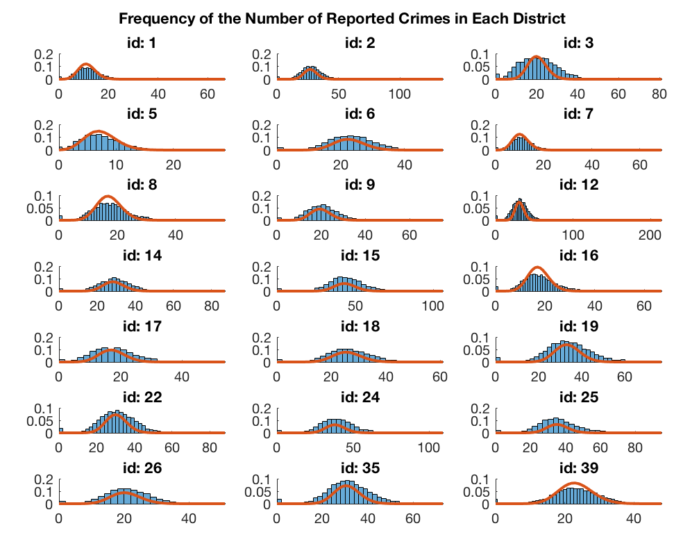
Figure 1: Frequencies of the number of reported crimes in each district in the Philadelphia Crime Incidents dataset. The red curves display the best Poisson fit to the data.

To create daily crime frequencies in Figure 1, we first calculate the daily counts of criminal incidents in each of the 21 geographical police districts in Philadelphia by grouping together all the crime reports with the same date; we then normalize these counts to get frequencies. Each subfigure in Figure 1 represents a police district. The horizontal axis of the subfigure corresponds to the number of reported incidents in a day and the vertical axis represents the frequency of each number on the horizontal axis. These frequencies approximate the true (marginal) distributions of the number of reported crimes in each of the districts in Philadelphia. Therefore, throughout this section we take these frequencies as the ground truth candidate distributions for the number of reported incidents in each of the districts.

Figure 1 shows that crime distributions in different districts can be quite different; e.g., the average number of daily reported incidents in District 15 is 43.5, which is much higher than the average of 11.35 in District 1 (see Table 1 in Appendix C for more details). Despite these differences, each of the crime distributions can be approximated well by a Poisson distribution. The red curves overlayed in each subfigure correspond to the Poisson distribution obtained via maximum likelihood estimation on data from that district. Throughout, we refer to such distributions as the best Poisson fit to the data (see Table 2 in Appendix C for details about the goodness of fit).

In our experiments, we take the police officers assigned to the districts as the resource to be distributed, the ground truth crime frequencies as candidate distributions, and aim to maximize the sum of the number of crimes discovered under the precision model of discovery.

4.2 Results

We can quantify the extent to which fairness degrades utility in the dataset through a notion we call Price of Fairness (PoF henceforth). In particular, given the ground truth crime distributions and the precision model of discovery, for a fairness level $\alpha$, we define $\text{PoF}(\alpha)=\chi(\textbf{w}^{*})/\chi(\textbf{w}^{\alpha})$. The PoF is simply the ratio of the expected number of crimes discovered by an optimal allocation to the expected number of crimes discovered by an optimal $\alpha$-fair allocation. Since $\chi(\textbf{w}^{*})\geq\chi(\textbf{w}^{\alpha})$ for all $\alpha$, the PoF is at least one. Furthermore, the PoF is monotonically non-increasing in $\alpha$. We can apply the algorithms given in Sections 3.1 and 3.2 respectively for computing optimal unconstrained, and optimal fair allocations with the with ground truth distributions as input and numerically compute the PoF. This is illustrated in Figure 2. The $x$ axis corresponds to different $\alpha$ values and the $y$ axis displays $1/\text{PoF}(\alpha)$. Each curve corresponds to a different number of total police officers denoted by $\mathcal{V}$. Because feasible allocations must be integral, there can sometimes be no feasible $\alpha$-fair allocation for small $\alpha$. Since the PoF in these cases is infinite we instead opt to display the inverse, $1/\text{PoF}$, which is always bounded in $[0,1]$. Higher values of inverse PoF are more desirable.

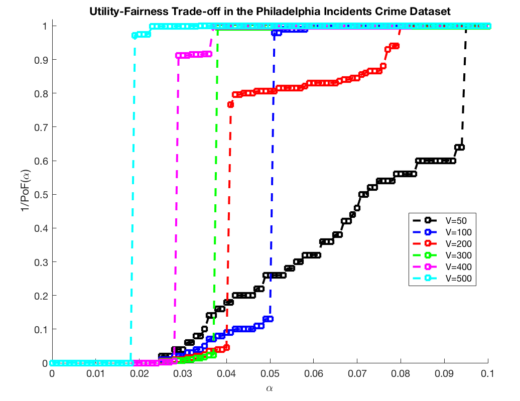
Figure 2: Inverse PoF plots for the Philadelphia Crime Incidents dataset. Smaller values indicate greater sacrifice in utility to meet the fairness constraint.

Figure 2 shows a diverse set of utility/fairness trade-offs depending on the number of available police officers. It also illustrates that the cost of fairness is rather low in most regimes. For example, in the worst case, with only 50 police officers (the black curve) (which is much smaller than the average number of daily reported crimes: 563.88), the inverse PoF is 1 for $\alpha\geq 0.1$, which corresponds to a 10% difference in the discovery probability across districts. When we increase the number of available police officers to 400 (the magenta curve), tolerating only a 4% difference in the discovery probability across districts is sufficient to guarantee no loss in the utility. Figure 2 also shows that for any fixed $\alpha$, the inverse $\text{PoF}(\alpha)$ tends to increase as the number of police increases (i.e. the cost of fairness decreases). This captures the intuition that fairness becomes a less costly constraint when resources are in greater supply. Finally, we observe a thresholding phenomenon in Figure 2; in each curve, increasing $\alpha$ beyond a threshold will significantly increase the inverse PoF. This is due to discretization effects, since only integral allocations are feasible.

We next turn into analyzing the performance of Algorithm 2 in practice. We run the algorithm instantiated to fit Poisson distributions, but use observations from the ground truth distribution at each round. As we have shown in Figure 1 and Table 2, the ground truth is well approximated by a Poisson distribution.

We measure the performance of Algorithm 2 as follows. First, we fix a police budget $\mathcal{V}$ and unfairness budget $\alpha$ and run Algorithm 2 for 2000 rounds using the dataset as the ground truth. That is, we simulate each round’s crime count realizations in each of the districts as being sampled from the ground truth distributions, and return censored observations under the precision model to Algorithm 2 according to the algorithm’s allocations and the drawn realizations. The algorithm returns an allocation after termination and we can measure the expected number of crimes discovered and fairness violation (the maximum difference in discovery probabilities over all pairs of districts) of the returned allocation using the ground truth distributions. Varying $\alpha$ while fixing $\mathcal{V}$ allows us to trace out the Pareto frontier of the utility/fairness trade-off for a fixed police budget. Similarly, for any fixed $\mathcal{V}$ and $\alpha$, we can run Algorithm 1 (the offline algorithm for computing an optimal fair allocation) with the ground truth distributions as input and trace out a Pareto curve by varying $\alpha$. We refer to these two Pareto curves by the learned and optimal Pareto curves, respectively. So to measure the performance of Algorithm 2, we can compare the learned and optimal Pareto curves.

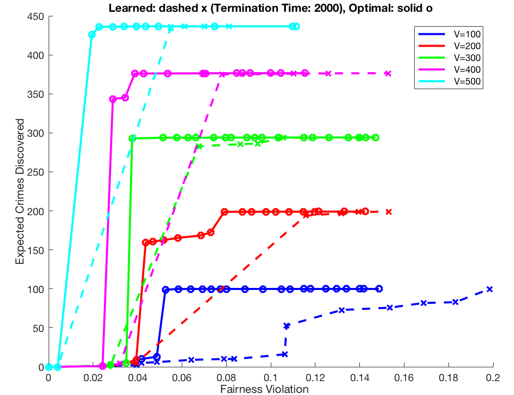
Figure 3: Pareto frontier of expected crimes discovered versus fairness violation.

In Figure 3, each curve corresponds to a police budget. The $x$ and $y$ axes represent the expected number of crimes discovered and fairness violation for allocations on the Pareto frontier, respectively. In our simulations we varied $\alpha$ between 0 and 0.15. For each police budget $\mathcal{V}$, the ‘x’ s connected by the dashed lines show the learning Pareto frontier. Similarly, the circles connected by solid lines show the optimal Pareto frontier. We point out that while it is possible for the fairness violations in the learned Pareto curves to be higher than the level of $\alpha$ set as an input to Algorithm 2, the fairness violations in the optimal Pareto curves are always bounded by $\alpha$.

The disparity between the optimal and learned Pareto curves are due to the fact that the learning algorithm has not yet fully converged. This can be attributed to the large number of censored observations received by Algorithm 2, which are significantly less informative than uncensored observations. Censoring happens frequently because the number of police used in every case plotted is less than the daily average of 563.88 crimes across all the districts in the dataset — so it is unavoidable that in any allocation, there will be significant censoring in at least some districts.

Figure 3 shows that while the learning curves are dominated by the optimal curves, the performance of the learning algorithm approaches the performance of the offline optimal allocation as $\mathcal{V}$ increases. Again, this is because increasing $\mathcal{V}$ generally has the effect of decreasing the frequency of censoring.

We study the $\mathcal{V}=500$ regime in more detail, to explore the empirical rate of convergence. In Figure 4, we study the round by round performance of the allocation computed by Algorithm 2 in a single run with the choice of $\mathcal{V}=500$ and $\alpha=0.05$.

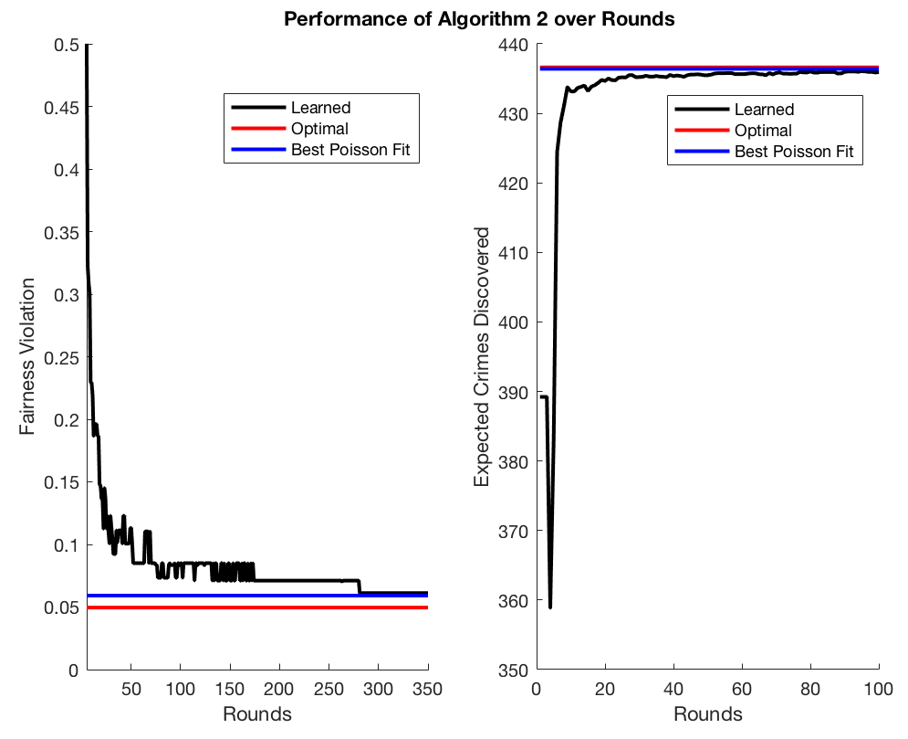
Figure 4: The per round expected number of crimes discovered and fairness violation of Algorithm 2. $\mathcal{V}=500$ and $\alpha=0.05$.

In Figure 4, the $x$ axis labels progression of rounds of the algorithm. The $y$ axis measures the fairness violation (left) and expected number of crimes discovered (right) of the allocation deployed by the algorithm, as measured with respect to the ground truth distributions. The black curves represent Algorithm 2. For comparison we also show the same quantities for an offline optimal fair allocation as computed with respect to the ground truth (red line), and an offline optimal fair allocation as computed with respect to the best Poisson fit to the ground truth (blue line). Note that in the limit, the allocations chosen by Algorithm 2 are guaranteed to converge to the blue baselines — but not the red baseline, because the algorithm is itself learning a Poisson approximation to the ground truth. The disparity between the red and blue lines quantifies the degradation in performance due to using Poisson approximations, rather than due to non-convergence of the learning process.

Figure 4 shows that Algorithm 2 converges to the Poisson approximation baseline well before the termination time of 2000, and substantially before the convergence bound guaranteed by our theory. Examining the estimated Poisson parameters used internally by Algorithm 2 reveals that although the allocation has converged to an optimal fair allocation, the estimated parameters have not yet converged to the parameters of the best Poisson fit in any of the districts. In particular, Algorithm 2 underestimates the parameters in all of the districts — but the degree of the underestimation is systematic: the correlation coefficient between the true and estimated parameters is $0.9975$.

We see also in Figure 4 that convergence to the optimum expected number of discovered crimes occurs more quickly than convergence to the target fairness violation level. This is also apparent in Figure 3 where the learning and optimal Pareto curves are generally similar in terms of the maximum number of crimes discovered, while the fairness violations are higher in the learning curves.

5 The Random Discovery Model

Finally, we consider the random model of discovery. In the random model, when $v_{i}$ units are allocated to a group with $c_{i}$ candidates, the number of discovered candidates is a random variable corresponding to the number of candidates that appear in a uniformly random sample of $v_{i}$ individuals from a group of size $m_{i}$. Equivalently, when $v_{i}$ units are allocated to a group of size $m_{i}$ with $c_{i}$ candidates, the number of candidates discovered by $\operatorname{disc}(\cdot)$ is a random variable $\operatorname{disc}(v_{i},c_{i})\triangleq o_{i},$ where $o_{i}$ is drawn from the hypergeometric distribution with parameters $m_{i}$, $c_{i}$ and $v_{i}$. Furthermore, the expected number of candidates discovered when allocating $v_{i}$ units to group $i$ is $\mathop{\mathbb{E}}[\operatorname{disc}(v_{i},c_{i})]=v_{i}\mathop{\mathbb{E}}[c_{i}]/m_{i}$.

For simplicity, throughout this section, we assume $m_{i}\geq\mathcal{V}$ for all $i$. This assumption can be completely relaxed (see the discussion in Appendix D). Moreover, let $\mu_{i}=\mathop{\mathbb{E}}[c_{i}]/m_{i}$ denote the expected fraction of candidates in group $i$. Without loss of generality, for the rest of this section, we assume $\mu_{1}\geq\mu_{2}\geq\ldots\geq\mu_{\mathcal{G}}$.

5.1 Optimal Allocation

In this section, we characterize optimal allocations. Note that the expected number of candidates discovered by the allocation choice $v_{i}\leq m_{i}$ in group $i$ is simply $v_{i}\mu_{i}$. This suggests a simple algorithm to compute $\textbf{w}^{*}$: allocating every unit of the resource to group 1. More generally, let $\mathcal{G}^{*}=\{i\mid\mu_{i}=\mu_{1}\}$ denote the subset of groups with the highest expected number of candidates. An allocation is optimal if and only if it only allocates all resources to groups in $\mathcal{G}^{*}$.

5.2 Properties of Fair Allocations

We next discuss the properties of fair allocations in the random discovery model. First, we point out that the discovery probability can be simplified as

$$f_{i}({v_{i}})=\mathop{\mathbb{E}}_{c_{i}\sim\mathcal{C}_{i}}\left[\frac{c_{i}v_{i}/m_{i}}{c_{i}}\right]=\frac{v_{i}}{m_{i}}.$$

So an allocation is $\alpha$-fair in the random model if $|v_{i}/m_{i}-v_{j}/m_{j}|\leq\alpha$ for all groups $i$ and $j$. Therefore, fair allocations (roughly) distribute resources in proportion to the size of the groups, essentially ignoring the candidate distributions within each group. We defer the full characterization to Appendix D.

5.3 Price of Fairness

Recall that PoF quantifies the extent to which constraining the allocation to satisfy $\alpha$-fairness degrades utility. While in Section 4 we study the PoF on the Philadelphia Crime Incidents dataset, we can define a worst-case variant as follows.

Definition 3.

Fix the random model of crime discovery and let $\alpha\in[0,1]$. We define the PoF as

$$\text{PoF}(\alpha)=\max_{\mathcal{C}}\frac{\chi(\textbf{w}^{*},\mathcal{C})}{\chi(\textbf{w}^{\alpha},\mathcal{C})}.$$

where $\mathcal{C}$ ranges over all possible candidate distributions.

We can fully characterize this worst-case PoF in the random discovery model. We defer the proof of Theorem 4 to Appendix D.

Theorem 4.

The PoF in the random discovery model is

$$\text{PoF}(\alpha)=\begin{cases}1,&\frac{\mathcal{V}}{m_{1}}\leq\alpha,\\ \frac{M}{m_{1}+\alpha(M-m_{1})},&\frac{\mathcal{V}}{m_{1}}>\alpha.\end{cases}$$

The PoF in the random model can be as high as $M/m_{1}$ in the worst case. If all groups are identically sized, this grows linearly with the number of groups.

6 Conclusion and Future Directions

Our presentation of allocative fairness provides a family of fairness definitions, modularly parameterized by a “discovery model”. What counts as “fair” depends a great deal on the choice of discovery model, which makes explicit what would otherwise be unstated assumptions about the process of tasks like policing. The random and precision models of discovery studied in this paper represent two extreme points of a spectrum. In the predictive policing setting, the random model of discovery assumes that officers have no advantage over random guessing when stopping individuals for further inspection. The precision model assumes they can oracularly determine offenders, and stop only them. An interesting direction for future work is to study discovery models that lie in between these two.

We have also made a number of simplifying assumptions that could be relaxed. For example, we assumed the candidate distributions are stationary — fixed independently of the actions of the algorithm. Of course, the deployment of police officers can change crime distributions. Modeling this kind of dynamics, and designing learning algorithms that perform well in such dynamic settings would be interesting. Finally, we have assumed that the same discovery model applies to all groups. One friction to fairness that one might reasonably conjecture is that the discovery model may differ between groups — being closer to the precision model for one group, and closer to the random model for another. We leave the study of these extensions to future work.

Acknowledgements

We thank Sorelle Friedler for giving a talk at Penn which initially inspired this work. We also thank Carlos Scheidegger, Kristian Lum, Sorelle Friedler, and Suresh Venkatasubramanian for helpful discussions at an early stage of this work. We thank Richard Berk and Greg Ridgeway for helpful discussions about predictive policing. Finally, we thank the anonymous reviewer for helpful comments regarding Figure 2.

Appendix A Feasibility in Expectation

In this section, we show how to compute $\textbf{w}^{\alpha}$ for any arbitrary but known candidate distributions $\mathcal{C}$ and known discovery model $\operatorname{disc}(\cdot)$ in a relaxation where the feasibility constraint is satisfied in expectation.

The first observation is that when $\operatorname{disc}(\cdot)$ and $\mathcal{C}$ are both known, for a group $i$ and allocation of $j$ units of resource to that group, the expected number of discovered candidates

$$\operatorname{disc}_{ij}=\mathop{\mathbb{E}}_{c_{i}\sim\mathcal{C}_{i}}\left[\operatorname{disc}(j,c_{i})\right],$$

and the discovery probability

$$f_{ij}=\mathop{\mathbb{E}}_{c_{i}\sim\mathcal{C}_{i}}\left[\frac{\operatorname{disc}(j,c_{i})}{c_{i}}\right],$$

can both be computed exactly. The second observation is that when allowing the feasibility condition to be satisfied in expectation, instead of allocating integral units of resources to each group, we can allocate resources to a group using a distribution.

Let $p_{ij}$ denote the probability that $j$ units of resource is allocated to group $i$. We can compute $\textbf{w}^{\alpha}$ by writing the following linear program with $p_{ij}$s as variables.

$$\max_{p_{ij}} \sum_{i\in[\mathcal{G}]}\sum_{j=1}^{\mathcal{V}}p_{ij}\operatorname{disc}_{ij},$$

subject to $$\sum_{i\in[\mathcal{G}]}\sum_{j=1}^{\mathcal{V}}p_{ij}j\leq\mathcal{V},$$

$$\left|\sum_{j=1}^{\mathcal{V}}p_{ij}f_{ij}-\sum_{j=1}^{\mathcal{V}}p_{i^{\prime}j}f_{i^{\prime}j}\right|\leq\alpha,\forall i\text{ and }i^{\prime}\in[\mathcal{G}],$$

$$\sum_{j=1}^{\mathcal{V}}p_{ij}=1,\forall j,$$

$$p_{ij}\geq 0,\forall i\text{ and }j.$$

The objective function maximizes the number of candidates discovered given the allocation. The first constraint guarantees that the allocation is feasible in expectation. The second constraint (which is linear in $p_{ij}$) ensures that $\alpha$-fairness is satisfied by the allocation. The last two constraints guarantees that for any $i$, $p_{ij}$ values define a valid probability distribution on all the possible allocations to group $i$.

Appendix B Omitted Details from Section 3

B.1 Omitted Details from Section 3.1

We first show how the expected number of discovered candidates in a group in the precision model can be written as a function of the tail probabilities of the group’s candidate distribution.

Lemma 5 (Ganchev et al. [13]).

The expected number of discovered candidates in the precision model when allocating $v_{i}$ units of resource to group $i$ can be written as $\mathop{\mathbb{E}}_{c_{i}\sim\mathcal{C}_{i}}[\min\left(c_{i},v_{i}\right)]=\Sigma_{c=1}^{v_{i}}\mathcal{T}_{i}(c)$.

Proof.

$$\mathop{\mathbb{E}}_{c_{i}\sim\mathcal{C}_{i}}\left[\min(c_{i},v_{i})\right] =\sum\limits_{c=1}^{m_{i}}\mathrm{Pr}_{c_{i}\sim\mathcal{C}_{i}}\left[c_{i}=c\right]\min(c,v_{i})=\sum\limits_{c=1}^{v_{i}-1}\mathrm{Pr}_{c_{i}\sim\mathcal{C}_{i}}\left[c_{i}=c\right]c+v_{i}\mathcal{T}_{i}(v_{i})$$

$$=\sum\limits_{c=1}^{v_{i}-2}\mathrm{Pr}_{c_{i}\sim\mathcal{C}_{i}}\left[c_{i}=c\right]c+(v_{i}-1)\mathcal{T}_{i}(v_{i}-1)+\mathcal{T}_{i}(v_{i})=\mathcal{T}_{i}(1)+\dots+\mathcal{T}_{i}(v_{i}-1)+\mathcal{T}_{i}(v_{i})$$

$$=\sum\limits_{c=1}^{v_{i}}\mathcal{T}_{i}(c).$$

Note that we can perform the telescoping in the 3rd and 4th lines by observing that $\mathrm{Pr}_{c_{i}\sim\mathcal{C}_{i}}\left[c_{i}=c-1\right]+\mathcal{T}_{i}(c)=\mathcal{T}_{i}(c-1).$ ∎

We then show that a greedy algorithm would find an optimal allocation in the precision model when the candidate distributions are known.

Theorem 5 (Theorem 1 in Ganchev et al. [13]).

The allocation returned by greedily allocating the next unit of resource to a group in

$$\operatorname*{arg\,max}\limits_{i\in[\mathcal{G}]}\left(\mathcal{T}_{i}(v_{i}^{t}+1)-\mathcal{T}_{i}(v_{i}^{t})\right),$$

where $v_{i}^{t}$ is the current allocation to group $i$ at the $t$^th round maximizes the expected number of candidates discovered.

Proof.

Since the tail probability functions $\mathcal{T}_{i}(c)$ are all non-increasing (that is, for $c\leq c^{\prime}$, we have $\mathcal{T}_{i}(c^{\prime})\leq\mathcal{T}_{i}(c)$), the greedy allocation returns an allocation v which maximizes

$$\chi(\textbf{v})=\sum\limits_{i\in[\mathcal{G}]}\sum\limits_{c=1}^{v_{i}}\mathcal{T}_{i}(c)\text{ such that }\sum_{i\in[\mathcal{G}]}v_{i}=\mathcal{V}.$$

Using Lemma 5 we have that

$$\sum\limits_{i\in[\mathcal{G}]}\mathop{\mathbb{E}}_{c_{i}\sim\mathcal{C}_{i}}\left[\min\left(c_{i},v_{i}\right)\right]=\sum\limits_{i\in[\mathcal{G}]}\sum_{c=1}^{v_{i}}\mathcal{T}_{i}(c).$$

So the above double-summation is exactly equal to the expected number of discovered candidates. To see that the greedy solution is optimal, notice that any solution which does not allocate the marginal resource to the tail with the highest remaining probability can be improved by reallocating the final allocated resource in some lower tail probability group to the one in the higher tail probability. Finally since each term in the objective function is non-negative an optimal allocation would use all the $\mathcal{V}$ units of resource (so the feasibility constraint is tight). ∎

B.2 Omitted Details from Section 3.2

Proof of Theorem 1.

Fix an optimal $\alpha$-fair allocation $\textbf{w}^{\alpha}$. In $\textbf{w}^{\alpha}$, some group $i$ has the highest $f_{i}$ and receives allocation $w^{\alpha}_{i}$. Suppose we know $i$ and $w^{\alpha}_{i}$ (we relax this assumption at the end of the proof). Using the knowledge of $\mathcal{C}_{i}$ we can compute $f_{i}(w^{\alpha}_{i})$. This implies that $f_{j}\in[f_{i}-\alpha,f_{i}]$ for every other group $j$, which in turn can be used to derive the set of all possible allowable allocations $w^{\alpha}_{j}$ which do not violate $\alpha$-fairness.

We claim that if we initialize the allocation $w^{\alpha}_{j}$ to be the lower bound of the interval corresponding to group $j$, then greedily assign the surplus units with the added restriction that $w^{\alpha}_{j}$ is always inside of its respective interval, we achieve an optimal $\alpha$-fair allocation.

Since we assume we know $w^{\alpha}_{i}$ to be the allocation to group $i$ in an optimal fair allocation, this allocation must be achievable by picking some value from each of the intervals, thus initializing the allocation to the lower bound of each interval certainly cannot assign more than $\mathcal{V}$ units in total. By the same argument as for the unconstrained greedy algorithm, since the objective function is concave (recall that the tail probabilities are non-increasing) and increasing in each argument $w^{\alpha}_{j}$, a greedy search over this feasible region finds the desired allocation.

The algorithm does not know a priori the group $i$ which has the maximum $f_{i}$ or $w^{\alpha}_{i}$, so it must search over these options. There are $\mathcal{G}$ guesses for group $i$ and $\mathcal{V}+1$ guesses for the allocation to the group. So there are a total of $\mathcal{G}(\mathcal{V}+1)$ guesses that needs to be considered. For each guess, it takes $O(M)$ to compute the upper and lower bounds on the allocation to each of the groups and $O(\mathcal{G}\mathcal{V})$ to run the greedy algorithm. So the running time of Algorithm 1 is $O(\mathcal{G}\mathcal{V}(\mathcal{G}\mathcal{V}+M))$. ∎

B.3 Omitted Details from Section 3.3

Proof of Theorem 2.

Let $i$ denote the group in which $\mathcal{A}$ has not allocated at least $m_{i}/2$ units for at least $k\ln(1/\delta)/(\alpha m_{i})$ rounds upon its termination. We fix an arbitrary allocation v and design two candidate distributions for group $i$ such that the discovery probabilities given $v_{i}$ computed under the two different distributions are at least 2$\alpha$-apart. Any algorithm guaranteeing $\alpha$-fairness must distinguish between these two distributions with high probability, or v could have higher unfairness than $\alpha$. We then show that to distinguish between these two candidate distributions, with probability of at least $1-\alpha$, any algorithm is required to send $m_{i}/2$ units to group $i$ for at least $k\ln(1/\delta)/(\alpha m_{i})$ rounds.

Consider two candidate distributions $\mathcal{C}_{i}$ and $\mathcal{C}^{\prime}_{i}$ for group $i$. We use the shorthand $p_{i}(c)=\mathrm{Pr}_{c_{i}\sim\mathcal{C}_{i}}[c_{i}=c]$ and similarly for $p^{\prime}_{i}(c)$. Let $c^{*}=m_{i}/2-2$. We require only that $\mathcal{C}_{i}$ and $\mathcal{C}^{\prime}_{i}$ satisfy the following conditions.

1. $p_{i}(c)=p^{\prime}_{i}(c)$ for all $c^{\prime}\leq c^{*}$.

2. $\Sigma_{c\leq c^{*}}p_{i}(c)=\Sigma_{c\leq c^{*}}p^{\prime}_{i}(c)=1-2\alpha m_{i}.$

3. $p_{i}(c^{*}+1)=2\alpha m_{i}$ and $p_{i}(c)=0$ for all $c\in\{c^{*}+1,\ldots,m_{i}\}$.

4. $p^{\prime}_{i}(c)=0$ for all $c\in\{c^{*}+1,\ldots,m_{i}-1\}$ and $p^{\prime}_{i}(m_{i})=2\alpha m_{i}$.

In other words, any two distributions that are the same up to $c^{*}$, have a CDF value of $2\alpha m_{i}$ at $c^{*}$, and differ in where in the tail they assign the remaining mass, will serve our purposes.

Let $f_{i}(v_{i})$ and $f^{\prime}_{i}(v_{i})$ denote the discovery probability given allocation v which assigns $v_{i}$ units to group $i$ for candidate distributions $\mathcal{C}_{i}$ and $\mathcal{C}^{\prime}_{i}$, respectively. Then

$$\left|f_{i}(v_{i})-f^{\prime}_{i}(v_{i})\right|=2\alpha m_{i}\left|\frac{v_{i}}{c^{*}+1}-\frac{v_{i}}{m_{i}}\right|.$$

This difference is minimized at $v_{i}=1$, in which case

$$\left|\frac{v_{i}}{c^{*}+1}-\frac{v_{i}}{m_{i}}\right|>\frac{2}{m_{i}}-\frac{1}{m_{i}}=\frac{1}{m_{i}}.$$

Hence, for any allocation v, $\left|f_{i}(v_{i})-f^{\prime}_{i}(v_{i})\right|>2\alpha.$

Finally, because $\mathcal{C}_{i}$ and $\mathcal{C}_{i}^{\prime}$ do not differ on any potential observation less than $c^{*}$, distinguishing between the two candidate distributions requires observing at least one uncensored observation of $c^{*}$ or higher. Under the precision model, this requires sending at least $m_{i}/2$ units to group $i$. However, conditioning on sending at least $m_{i}/2$ units, the probability of observing an uncensored observation is at most $2\alpha m_{i}$. Hence, to distinguish between $\mathcal{C}_{i}$ and $\mathcal{C}_{i}^{\prime}$ (and thus to guarantee that an allocation v is $\alpha$-fair) with probability of at least $1-\delta$, a learning algorithm must allocate $m_{i}/2$ units for $k\ln(1/\delta)/(\alpha m_{i})$ rounds to group $i$. ∎

B.4 Omitted Details from Section 3.4

Since in our analysis we consider the groups separately, we fix a group $i$ throughout the rest of this section and drop the subscript $i$ for convenience. Our first lemma shows that the true underlying parameter $\lambda^{*}$ uniquely maximizes $\mathop{\mathbb{E}}[\ell]$ for any allocation. Since $\mathcal{L}^{*}$ is just a sum of $\mathop{\mathbb{E}}[\ell]$ terms, it follows as a corollary that $\mathcal{L}^{*}$ is uniquely maximized at $\lambda^{*}$ for any sequence of allocations. This is stated as Lemma 6 and Corollary 1.

Lemma 6.

For any $v$, $\operatorname*{arg\,max}_{\lambda}\mathop{\mathbb{E}}_{o}[\ell(v,o;\lambda)]=\{\lambda^{*}\}.$

Proof.

Notice that since the expected log-likelihood function is the average over time periods of individual $\ell(v_{i}^{t},c_{i}^{t},\lambda)$ terms, $\lambda^{*}$ being the unique maximizer of each term individually will imply that it is the unique maximizer of the the expected log-likelihood function. Thus we aim to show that

$$\mathop{\mathbb{E}}\left[\ell\left(v^{t},o^{t},\lambda^{*}\right)\right] >\mathop{\mathbb{E}}\left[\ell\left(v^{t},o^{t},\lambda\right)\right].$$

Notice that this is true if and only if

$$\mathop{\mathbb{E}}\left[-\log\left(\frac{p(v^{t},o^{t},\lambda)}{p(v^{t},o^{t},\lambda^{*})}\right)\right]>0.$$ (5)

Recall the Gibb’s inequality, written here for the discrete case as in MacKay [22].

Lemma 7.

Suppose $p$ and $q$ are two discrete distributions. Let $D_{KL}(p||q)$ denote the KL divergence between $p$ and $q$. Then $D_{KL}(p||q)\geq 0$ with equality if and only if $p(x)=q(x)$ for all $x$.

So the quantity in Equation 5 is the KL divergence between two distributions. Since the distributions place different probabilities on at least one event (in fact, infinitely many events), the inequality is strict by Lemma 7. ∎

Corollary 1.

For any $\textbf{h}^{t}$, $\operatorname*{arg\,max}_{\lambda}\mathcal{L}^{*}(\lambda,\textbf{h}^{t})=\{\lambda^{*}\}.$

Lemma 8.

$\left|\ell\left(v^{t},o^{t};\lambda\right)\right|\leq\max\left(\left|\ell\left(\mathcal{V},\mathcal{V};\lambda_{\min}\right)\right|,\left|\ell\left(\mathcal{V}-1,\mathcal{V};\lambda_{\min}\right)\right|,\left|\ell\left(1,0;\lambda_{\max}\right)\right|\right).$

Proof.

The Poisson’s PMF is unimodal and achieves its maximum at $\lambda$, where $p(v^{t},o^{t};\lambda)$ will be at most 1, meaning $\ell(v^{t},o^{t};\lambda)\leq 0$. So, in order to bound the absolute value, we will bound how small $\ell$ can get.

We prove the claim by a case analysis. For uncensored observations, the minimum log-likelihood is achieved at either $0$ or at $\mathcal{V}-1$ due to unimodality. In this case, the choice of $\lambda$ that can result in the minimum value is at $\lambda_{\max}$ or $\lambda_{\min}$, respectively. In the case of a censored observation, $\ell(v^{t},o^{t};\lambda)=\log(1-F(v^{t}-1;\lambda)).$ So the minimum will be achieved at $\ell(\mathcal{V},\mathcal{V};\lambda_{\min})$. ∎

Next we show that for any fixed $\lambda$, with high probability over the randomness of $\{o^{t}\}$, $\hat{\mathcal{L}}$ converges to $\mathcal{L}^{*}$ for any sequence of allocations $\{v^{t}\}$ that Algorithm 2 could have chosen.

Lemma 9.

For any $\lambda\in[\lambda_{min},\lambda_{max}]$ and any $\textbf{h}^{t}$

$$\mathrm{Pr}\left[\left|\hat{\mathcal{L}}(\textbf{h}^{t},\lambda)-\mathcal{L}^{*}(\textbf{h}^{t},\lambda)\right|>\epsilon\right]\leq 2e^{-\frac{t\epsilon^{2}}{2C^{2}}},$$

where $C$ is a constant and in the case of Poisson distribution

$$C=\frac{1}{2}max\Big{(}\left|\ell\left(\mathcal{V},\mathcal{V};\lambda_{min}\right)\right|,\left|\ell\left(\mathcal{V}-1,\mathcal{V};\lambda_{min}\right)\right|,\left|\ell\left(1,0;\lambda_{max}\right)\right|\Big{)}.$$

Proof.

With a slight abuse of notation, let $\mathcal{A}(h^{s})$ denote the allocation to the group we are considering. We define $Q^{t}$ as follows.

$$Q^{t} :=t\left(\hat{\mathcal{L}}\left(\textbf{h}^{t},\lambda\right)-\mathcal{L}^{*}\left(\textbf{h}^{t},\lambda\right)\right)=\sum_{s=1}^{t}\ell\left(\mathcal{A}(h^{s}),o^{s};\lambda\right)-\sum_{s=1}^{t}\mathop{\mathbb{E}}\left[\ell\left(\mathcal{A}(h^{s}),o^{s};\lambda\right)\right].$$

So $Q^{t}$ is the sum of the difference between each period’s observed and expected conditional log-likelihood function. Notice that $Q^{t}$ is a martingale, as $\mathop{\mathbb{E}}[Q^{t+1}|Q^{t}]=Q^{t}$. Moreover, its terms form a bounded difference sequence since $\ell(\mathcal{A}(h_{s}),o^{s};\lambda)$ is continuous in $o^{s}_{i}$ with $o^{s}_{i}\in[0,\mathcal{V}]$ and $\lambda\in[\lambda_{\min},\lambda_{\max}]$. In particular, we show in Lemma 8 that $\ell(v^{t},o^{t};\lambda)|\leq 2C$.

Since $\{Q^{t}\}$ is a bounded martingale difference sequence, we can apply Azuma’s inequality to get

$$\mathrm{Pr}\left[\left|Q^{t}-Q^{0}\right|\geq t\epsilon\right]\leq 2e^{-\frac{t\epsilon^{2}}{2C^{2}}}.$$

Rearranging gives the claim. ∎

For $k$ values of $\lambda$, taking the union bound and setting $\epsilon=\sqrt{2C^{2}\ln(2k\mathcal{G}/\delta)/t}$ provides the following corollary.

Corollary 2.

Let $\Lambda$ be a set of $k$ values such that for any $\lambda\in\Lambda$, $\lambda\in[\lambda_{\min},\lambda_{\max}]$. Then with probability at least $1-\delta/\mathcal{G}$

$$\max_{\lambda\in\Lambda}\left|\hat{\mathcal{L}}(\textbf{h}^{t},\lambda)-\mathcal{L}^{*}(\textbf{h}^{t},\lambda)\right|\leq\sqrt{\frac{2C^{2}\ln(\frac{2k\mathcal{G}}{\delta})}{t}},$$

where $C$ is as in Lemma 9.

Lemma 10.

For any $\lambda$, $\lambda^{\prime}\in[\lambda_{\min},\lambda_{\max}]$ such that $|\lambda-\lambda^{\prime}|<\epsilon$, we have that $|\ell(v^{t},o^{t};\lambda)-\ell(v^{t},o^{t};\lambda^{\prime})|\leq b\epsilon$ for some constant $b$.

Proof.

Recall that a differentiable function is Lipschitz-continuous if and only if its derivative is bounded. By definition,

$$\ell\left(v^{t}o^{t};\lambda\right):=\begin{cases}\log\left(\frac{e^{-\lambda}\lambda^{o^{t}}}{o^{t}!}\right),&o^{t}<v^{t},\\ \log\left(1-F\left(v^{t}-1;\lambda\right)\right),&\text{otherwise.}\end{cases}$$

So we can analyze the derivative by cases.

In the uncensored case ($o^{t}<v^{t}$), we have that

$$\ell\left(v^{t},o^{t},\lambda\right)=-\lambda+o^{t}\log\lambda-\log o^{t}!\implies\frac{\partial\ell}{\partial\lambda}=-1+\frac{o^{t}}{\lambda}.$$

For $\lambda\in[\lambda_{\min},\lambda_{\max}]$ with $\lambda_{\min}>0$, this function is continuous and its domain is bounded. Hence its image is bounded and

In the censored case ($o^{t}=v^{t}$), we can write that

$$\ell\left(v^{t},o^{t};\lambda\right) =\log\left(1-F\left(v^{t}-1;\lambda\right)\right)=\log\left(\sum_{k=v^{t}}^{\infty}\frac{\lambda^{k}e^{-\lambda}}{k!}\right)=-\lambda+\log\left(\sum_{k=v^{t}}^{\infty}\frac{\lambda^{k}}{k!}\right).$$

Again taking the derivative, we get

$$\frac{\partial\ell}{\partial\lambda}=-1+\frac{\frac{\partial}{\partial\lambda}\sum_{k=v^{t}}^{\infty}\frac{\lambda^{k}}{k!}}{\sum_{k=v^{t}}\frac{\lambda^{k}}{k!}} =-1+\frac{\frac{\partial}{\partial\lambda}\left[e^{\lambda}-\sum_{k=0}^{v^{t}-1}\frac{\lambda^{k}}{k!}\right]}{\sum_{k=v^{t}}^{\infty}\frac{\lambda^{k}}{k!}}=-1+\frac{\lambda-\sum_{k=1}^{v^{t}-1}\frac{\lambda^{k-1}}{(k-1)!}}{\frac{\lambda^{k}}{k!}}.$$

The fraction is the quotient of two continuous functions and the denominator is nonzero for any $\lambda\in[\lambda_{\min},\lambda_{\max}]$. So $\partial\ell/\partial\lambda$ is continuous in $\lambda$. Since the image of a continuous function on a compact set remains compact, $\partial\ell/\partial\lambda$ is bounded for all $t$. Thus $\ell(v^{t},o^{t};\lambda)$ is Lipschitz-continuous in this case as well. ∎

Proof of Lemma 1.

Define the $\epsilon$-net as $N_{\epsilon}=\{\lambda_{\min},\lambda_{\min}+\epsilon,\lambda_{\min}+2\epsilon,\dots,\lambda_{\max}\}.$ We use $k=|N_{\epsilon}|$ to denote the cardinality of the set; so $k=\lceil\lambda_{\max}-\lambda_{\min}\rceil/\epsilon$. Note that for any $\lambda\in[\lambda_{\min},\lambda_{\max}]$, there exists $\lambda^{\prime}\in N_{\epsilon}$ such that $|\lambda-\lambda^{\prime}|\leq\epsilon$.

By Corollary 2, for $\Lambda=\{\lambda_{1},\lambda_{2},\dots,\lambda_{k}\}$, with probability $1-\delta$,

$$\max_{\lambda\in\Lambda}\left|\hat{\mathcal{L}}\left(\textbf{h}^{t},\lambda\right)-\mathcal{L}^{*}\left(\textbf{h}^{t},\lambda\right)\right|\leq\sqrt{\frac{2C^{2}}{t}\ln\left(\frac{2k\mathcal{G}}{\delta}\right)}.$$ (6)

Now, for any $\lambda\in[\lambda_{\min},\lambda_{\max}]$ by triangle inequality we have that

$$\left|\hat{\mathcal{L}}\left(\textbf{h}^{t},\lambda\right)-\mathcal{L}^{*}\left(\textbf{h}^{t},\lambda\right)\right|\leq \left|\hat{\mathcal{L}}\left(\textbf{h}^{t},\lambda\right)-\hat{\mathcal{L}}\left(\textbf{h}^{t},\lambda^{\prime}\right)\right|+\left|\hat{\mathcal{L}}\left(\textbf{h}^{t},\lambda^{\prime}\right)-\mathcal{L}^{*}\left(\textbf{h}^{t},\lambda^{\prime}\right)\right|+\left|\mathcal{L}^{*}\left(\textbf{h}^{t},\lambda^{\prime}\right)-\mathcal{L}^{*}\left(\textbf{h}^{t},\lambda\right)\right|.$$

By Lemma 10, the first and third term are at most $\epsilon b$ where $b$ is again the Lipschitz constant in Lemma 10. Applying this to the closest $\lambda_{k}\in N_{\epsilon}$ and noting that the inequality in Equation 6 binds on the middle term with $C$ as in Lemma 9, we have

$$\left|\hat{\mathcal{L}}\left(\textbf{h}^{t},\lambda\right)-\mathcal{L}^{*}\left(\textbf{h}^{t},\lambda\right)\right| \leq\epsilon b+\sqrt{\frac{2C^{2}\ln\left(\frac{2k\mathcal{G}}{\delta}\right)}{t}}+\epsilon b\leq 2\epsilon b+\sqrt{\frac{2C^{2}\ln\left(\frac{2k\mathcal{G}}{\delta}\right)}{t}}\leq 2\epsilon b+\sqrt{\frac{2C^{2}\ln\left(\frac{2\mathcal{G}\lceil\lambda_{\max}-\lambda_{\min}\rceil}{\epsilon\delta}\right)}{t}}.$$

Setting $\epsilon=1/t$ yields the claim. Note that as $t\to\infty$, the difference approaches not only constant but diminishes to $0$. ∎

Lemma 11.

Suppose that a continuous function $g(x):[a,b]\mapsto\mathbb{R}$ has a unique maximizer $x^{*}$. Then for every $\epsilon>0,\ \exists\eta>0$ such that $g(x^{*})-g(x)<\eta$ implies $|x-x^{*}|<\epsilon$. In particular, this $\eta$ can be written as

$$g(x^{*})-\underset{x\in[a,x^{*}-\epsilon]\cup[x^{*}+\epsilon,b]}{\max}g(x).$$

When $g$ is concave and differentiable, $\eta$ can be evaluated by evaluating $g$ at a constant number of points.

Proof.

Let $X_{\epsilon}$ be the $\epsilon$-radius open ball centered at $x^{*}$, and let $\Theta$ be $[a,b]\setminus X_{\epsilon}$ i.e. the domain of $g$ excluding the $\epsilon$-radius ball centered at the maximizer. Since $X_{\epsilon}$ is open, $\Theta$ is closed and bounded, and therefore compact. Since $g$ is continuous, the restriction of $g$ to $\Theta$ has some maximum $g(\hat{x})$ for some (not necessarily unique) $\hat{x}\in\Theta$.

Observe that, if for any $x\in[a,b]$, we have that $g(x)>g(\hat{x})$, then $x$ must be in $X_{\epsilon}$. Otherwise $\hat{x}$ would not be a maximizer of the restriction of $f$ to $\Theta$. Choose $\eta=g(x^{*})-g(\hat{x})$. Then, because $g(x)>g(\hat{x})$, we have that $g(x^{*})-g(x)<g(x^{*})-g(\hat{x})=\eta$. Therefore, $|g(x^{*})-g(x)|<\eta$ implies $|x^{*}-x|<\epsilon$ , completing the proof of existence.

The dependence of $\eta$ on $\epsilon$ is function-dependent, but by construction, $\eta(\epsilon)$ can be computed by taking the maximum of $g$ on $\Theta\setminus X_{\epsilon}$ and subtracting it from $g(x^{*})$. Notice that in the case of concavity and differentiability, this maximization problem is easy to calculate. If $g$ is concave and differentiable over $[a,b]$, its restrictions to $[a,x^{*}-\epsilon]$ and $[x^{*}+\epsilon,b]$ are as well. A differentiable, concave function on an interval can only be maximized at an interior critical point or at one of the two end points. Hence if $x^{*}$ is interior, it must be a critical point, and by concavity it is the unique critical point on $[a,b]$, so $g$ can have no critical points on $\Theta\setminus X_{\epsilon}$. Thus $g$ restricted to $[a,x^{*}-\epsilon]$ is maximized at either $a$ or $x^{*}-\epsilon$; similarly for $g$ restricted to $[x^{*}+\epsilon,b]$. On the other hand, if $x^{*}$ is either $a$ or $b$, there is just one interval in $\Theta\setminus X_{\epsilon}$ to check, and checking the endpoints of that interval plus exhaust the possible maximizers. In either case, no more than 4 points need be checked; in contrast, without concavity or differentiability, finding the maximum on $g$ on $\Theta\setminus X_{\epsilon}$ could require more involved optimization techniques. ∎

Corollary 3.

For any fixed $\textbf{h}^{t}$ and $\lambda\in[\lambda_{min},\lambda_{max}]$, the following must hold true for $\mathcal{L}^{*}(\textbf{h}^{t},\lambda)$ whose unique maximizer is $\lambda^{*}$. For every $\epsilon,\ \exists\eta>0$ such that $\mathcal{L}^{*}(\textbf{h}^{t},\lambda^{*})-\mathcal{L}^{*}(\textbf{h}^{t},\lambda)<\eta$ implies $|\lambda-\lambda^{*}|<\epsilon$, where $\eta$ is

$$\mathcal{L}^{*}(\textbf{h}^{t},\lambda^{*})-\underset{\lambda\in[\lambda_{min},\lambda^{*}-\epsilon]\cup[\lambda^{*}+\epsilon,\lambda_{max}]}{\max}\mathcal{L}^{*}(\textbf{h}^{t},\lambda).$$

Fixing any group, we show that for any fixed allocation $v$, the difference between the discovery probability with respect to the true and estimated candidate distributions is proportional to the total variation distance between the true and estimated distributions.

Lemma 12.

Let $v$ be any fixed allocation to the group. Then $\left|f(v,\mathcal{C}(\lambda^{*}))-f(v,\mathcal{C}(\hat{\lambda}))\right|\leq 2D_{TV}(\mathcal{C}(\lambda^{*}),\mathcal{C}(\hat{\lambda})).$

Proof.

$$\left|f(v,\mathcal{C}(\lambda^{*}))-f(v,\mathcal{C}(\hat{\lambda}))\right| =\left|\mathop{\mathbb{E}}_{c\sim\mathcal{C}(\lambda^{*})}\left[\frac{\min(v,c)}{c}\right]-\mathop{\mathbb{E}}_{\textbf{c}\sim\mathcal{C}(\hat{\lambda})}\left[\frac{\min(v,c)}{c}\right]\right|=\left|\sum_{c=0}^{\infty}\frac{\min(v,c)}{c}\left(\mathrm{Pr}[c;\lambda^{*}]-\mathrm{Pr}[c;\hat{\lambda}]\right)\right|$$

$$\leq\sum_{c=0}^{\infty}\frac{\min(v,c)}{c}\left|\mathrm{Pr}[c;\lambda^{*}]-\mathrm{Pr}[c;\hat{\lambda}]\right|\leq\sum_{c=0}^{\infty}\left|\mathrm{Pr}[c;\lambda^{*}]-\mathrm{Pr}[c;\hat{\lambda}]\right|$$

$$\leq 2D_{TV}(\mathcal{C}(\lambda^{*}),\mathcal{C}(\hat{\lambda})).$$

∎

Appendix C Omitted Details from Section 4

Table 1 represents the average and standard deviation of the number of daily reported incidents in all of the districts in the Philadelphia Crime Incidents dataset.

id	average	standard deviation
1	11.35	5.1
2	27.44	9.24
3	20.37	9.27
5	7.36	3.65
6	22.67	7.54
7	10.47	4.56
8	17.26	6.77
9	19.83	7.15
12	30.97	10.86
14	28.69	9
15	43.5	12.69
16	17.36	6.99
17	17.41	7.45
18	25.88	8.35
19	33.43	10.71
22	30.45	9.89
24	38.47	11.82
25	35.54	12.41
26	20.55	7.16
35	30.92	9.79
39	23.24	7.16

Table 1: The average and standard deviation in the ground truth distributions in each of the districts of the Philadelphia Crime Incidents dataset.

Table 2 displays the $\ell_{1}$ and $\ell_{\infty}$ distances of the ground truth and best Poisson fit distribution for all of the districts in the Philadelphia Crime Incidents dataset. Observe that the $\ell_{\infty}$ metric shows that the Poisson fit provides a close approximation for the ground truth distribution. Also as Figure 1 displays, the Poisson fit is a better approximation to the ground truth had we ignored the 0 counts (the frequency of the days in which no crime has been reported) in the dataset. This metric has also been measured in Table 2 in the “no zero” columns. Note that the goodness of fit would improve significantly when removing the 0 counts according to the $\ell_{1}$ measure but would not change at all according to the $\ell_{\infty}$ measure.

id	$\ell_{1}$	$\ell_{1}$ (no zero)	$\ell_{\infty}$	${\ell_{\infty}}$ (no zero)
1	0.1656	0.1562	0.0315	0.0315
2	0.2021	0.1928	0.0293	0.0293
3	0.3420	0.3327	0.0493	0.0493
5	0.1203	0.1093	0.0328	0.0328
6	0.1853	0.1760	0.0309	0.0309
7	0.1269	0.1175	0.0279	0.0279
8	0.1835	0.1742	0.0365	0.0365
9	0.2025	0.1931	0.0315	0.0315
12	0.2600	0.2507	0.0304	0.0304
14	0.2024	0.1931	0.0239	0.0239
15	0.2305	0.2212	0.0276	0.0276
16	0.2024	0.1931	0.0354	0.0354
17	0.2495	0.2402	0.0436	0.0436
18	0.1953	0.1860	0.0278	0.0278
19	0.2494	0.2401	0.0337	0.0337
22	0.2469	0.2375	0.0326	0.0326
24	0.2529	0.2436	0.0284	0.0284
25	0.2844	0.2751	0.0312	0.0312
26	0.1896	0.1803	0.0328	0.0328
35	0.2187	0.2095	0.0291	0.0291
39	0.1478	0.1385	0.0243	0.0243
average	0.2123	0.2029	0.0319	0.0319

Table 2: Various statistical distances between the ground truth distribution and best Poisson fit for each of the districts.

In Figure 5 we compare the Pareto frontiers for the optimal and fitted curves. Figure 5 shows that the performance (in terms of the utility/fairness trade-off) does not degrade significantly when we assume the Philadelphia Crime Incidents dataset is generated according to Poisson distributions.

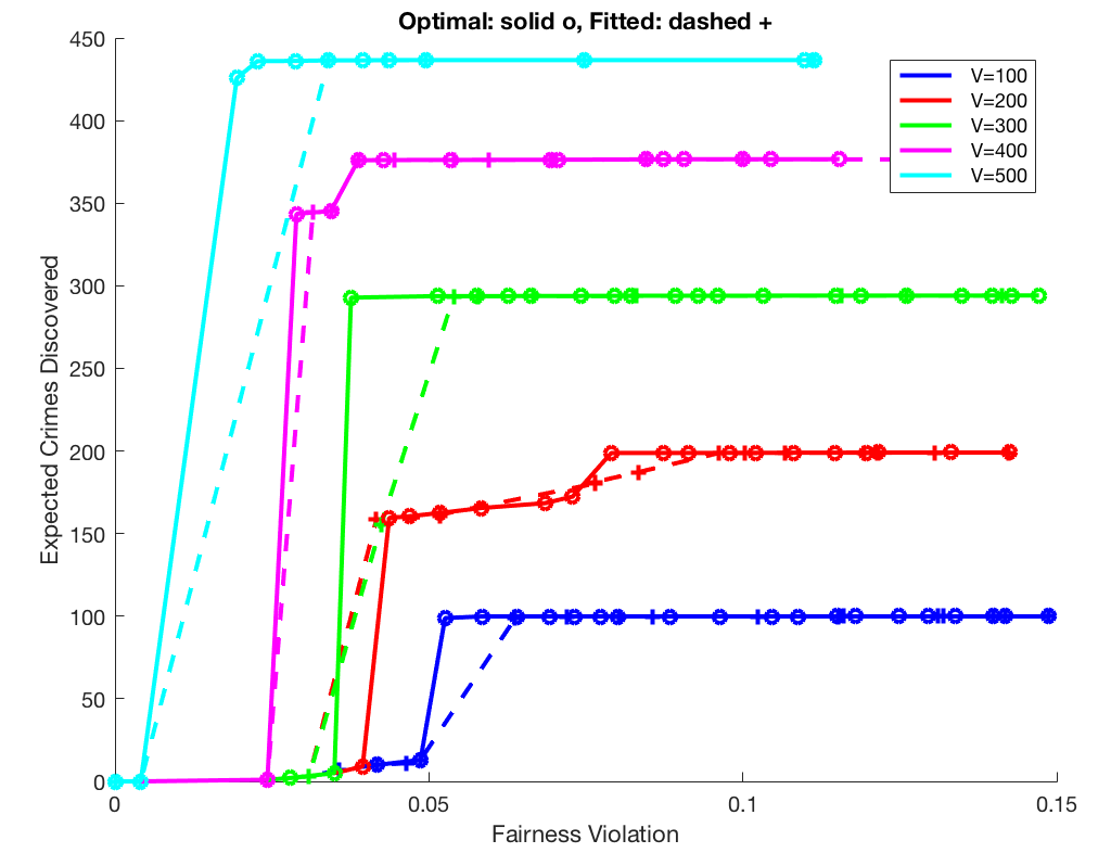
Figure 5: Pareto frontier of the expected crimes discovered versus fairness violation.

Appendix D Omitted Details From Section 5

First, we write down the integer programming to compute an optimal $\alpha$-fair allocation in the random model described in Section 5.2.

$$\underset{\textbf{v}=\{v_{1},\ldots,v_{\mathcal{G}}\}}{\max} \sum_{i=1}^{\mathcal{G}}\frac{v_{i}\mathop{\mathbb{E}}[c_{i}]}{m_{i}},$$

subject to $$\left|\frac{v_{i}}{m_{i}}-\frac{v_{j}}{m_{j}}\right|\leq\alpha,\forall i\text{ and }j,$$

$$\sum_{i=1}^{\mathcal{G}}v_{i}\leq\mathcal{V},$$

$$v_{i}\in\mathbb{N},\forall i.$$

Next we present the proof of Theorem 4.

Proof of Theorem 4.

Observe that when $\mathcal{V}/m_{1}\leq\alpha$ the allocation that sends all of the units of the resource to group 1 is both optimal and $\alpha$-fair. For the case that $\mathcal{V}/m_{1}>\alpha$, we will first provide an upper bound on the PoF by providing some allocation v, which is is $\alpha$-fair, and use that to show fairness does not deteriorate the total number of candidates discovered by v compared to an optimal $\alpha$-fair allocation. And then, we will construct a specific candidate distributions $\mathcal{C}^{\prime}$ and compute the PoF to show that the upper bound is tight.

Consider the following allocation v.

$$v_{i}=\begin{cases}\left(\frac{\mathcal{V}+\alpha(M-m_{1})}{M}\right)m_{1},&i=1,\\ \left(\frac{\mathcal{V}-\alpha m_{1}}{M}\right)m_{i},&\text{otherwise}.\end{cases}$$ (7)

We show that v is a feasible $\alpha$-fair allocation. To show feasibility, observe that

$$\sum_{i\in[\mathcal{G}]}v_{i} =\frac{\mathcal{V}-\alpha m_{1}}{M}\sum_{i\in[\mathcal{G}]}m_{i}+\alpha m_{1}=\mathcal{V}.$$

To show that v is $\alpha$-fair observe that

$$\left|f_{1}(v_{1})-f_{i}(v_{i})\right| =\left|\frac{v_{1}}{m_{1}}-\frac{v_{i}}{m_{i}}\right|=\left|\frac{\mathcal{V}+\alpha(M-m_{1})}{M}-\frac{\mathcal{V}-\alpha m_{1}}{M}\right|=\alpha\text{ and }\left|f_{i}(v_{i})-f_{j}(v_{j})\right|=0,\forall i,j\neq 1.$$

Since v is a feasible $\alpha$-fair allocation, for any $\mathcal{C}$, we have that

$$\chi(\textbf{w}^{\alpha},\mathcal{C})\geq\chi(\textbf{v},\mathcal{C})\geq\mu_{1}v_{1},$$

where the last inequality is derived by counting only the candidates that allocation v discovers in group $1$ according to the random model and ignoring all the discoveries in other groups. Moreover, for any $\mathcal{C}$, $\chi(\textbf{w}^{*},\mathcal{C})=\mu_{1}\mathcal{V}$ by the argument in Section 5.1. Therefore,

PoF $$=\max_{\mathcal{C}}\frac{\chi(\textbf{w}^{*},\mathcal{C})}{\chi(\textbf{w}^{\alpha},\mathcal{C})}\leq\frac{\mu_{1}\mathcal{V}}{\mu_{1}v_{1}}=\frac{\mathcal{V}M}{m_{1}\left(\mathcal{V}+\alpha(M-m_{1})\right)}\leq\frac{M}{m_{1}+\alpha(M-m_{1})},$$

where the last inequality uses the assumption that $\mathcal{V}\leq m_{1}$.

To derive the lower bound on the PoF, we construct a candidate distribution $\mathcal{C}^{\prime}$ and compute the PoF. We show that our lower on PoF matches the upper bound, so our analysis on PoF is tight.

To construct $\mathcal{C}^{\prime}$ assume all groups have size $\mathcal{V}$ i.e. $m_{i}=\mathcal{V}$ for all $i$. Furthermore, assume group 1 has $\mathcal{V}$ candidates and the rest of the groups have 0 candidates deterministically. Then the optimal allocation $\textbf{w}^{*}$ is to send all the $\mathcal{V}$ units of resource to group 1, and doing so will discover $\mathcal{V}$ candidates (since $\mu_{1}=1$). As for the optimal $\alpha$-fair allocation, we show that $\textbf{w}^{\alpha}=\textbf{v}$ where v is the same allocation as the allocation used in our upper bound (see Equation 7).

Lemma 13.

For $\mathcal{C}^{\prime}$, $\textbf{w}^{\alpha}=\textbf{v}$ where v is defined in Equation 7.

Proof.

For $\mathcal{C}^{\prime}$, because all groups have the same size, $v_{i}=v_{j}$ for all $i,j\neq 1$. Since $\Sigma_{i\in[\mathcal{G}]}v_{i}=\mathcal{V}$, $v_{i}=(\mathcal{V}-v_{1})/(\mathcal{G}-1)$ for all $i\neq 1$. Now, any feasible $\alpha$-fair allocation $\textbf{v}^{\prime}$ must have $v^{\prime}_{1}\leq v_{1}$. Assume by the way of contradiction that $v^{\prime}_{1}>v_{1}$. Then, after assigning $v^{\prime}_{1}$ units of resource to group 1, the remaining units that will be strictly less than $\mathcal{V}-v_{1}$ will be distributed among the remaining $\mathcal{G}-1$ groups. By the pigeonhole principle, there must exist at least one group $j$ such that

$$v^{\prime}_{j}<\frac{\mathcal{V}-v_{1}}{\mathcal{G}-1}=v_{j}=\left(\frac{\mathcal{V}-\alpha m_{1}}{M}\right)m_{j}.$$

Now observe that

$$\left|f_{1}(v^{\prime}_{1})-f_{j}(v^{\prime}_{j})\right| =\left|\frac{v^{\prime}_{1}}{m_{1}}-\frac{v^{\prime}_{j}}{m_{j}}\right|>\left|\frac{\mathcal{V}+\alpha(M-m_{1})}{M}-\frac{\mathcal{V}-\alpha m_{1}}{M}\right|=\alpha.$$

So $\textbf{v}^{\prime}$ cannot be $\alpha$-fair. Therefore, v must be an optimal $\alpha$-fair allocation since in v the maximum number of units of resources are allocated to group 1 which is the only group that contains candidates. ∎

Note that the number of candidates discovered by $\textbf{w}^{\alpha}$ is exactly $v_{1}$ since $\mu_{1}=1$. So given the $\textbf{w}^{\alpha}$ for $\mathcal{C}^{\prime}$ we can compute the PoF as follows.

PoF $$=\frac{\chi(\textbf{w}^{*},\mathcal{C}^{\prime})}{\chi(\textbf{w}^{\alpha},\mathcal{C}^{\prime})}=\frac{\mathcal{V}}{v_{1}}=\frac{\mathcal{V}M}{\left(\mathcal{V}+\alpha(M-m_{1})\right)m_{1}}=\frac{m_{1}M}{\left(m_{1}+\alpha(M-m_{1})\right)m_{1}}=\frac{M}{m_{1}+\alpha(M-m_{1})}.$$

This lower bounds matches our upper bound so our analysis on PoF is tight. ∎

D.1 Relaxing the Assumption of $\mathcal{V}\leq m_{i}$.

In this section we relax the assumption that $\mathcal{V}\leq m_{i}$ for all groups $i$. We first show how an optimal allocation can be computed using a greedy algorithm. Recall that we have assumed $\mu_{1}\geq\mu_{2}\geq\ldots\geq\mu_{\mathcal{G}}$. Optimal algorithm allocates $v_{1}=\min(\mathcal{V},m_{1})$ units of resource to group 1. And recurse with the remaining $\mathcal{V}-v_{1}$ resources on the rest of the groups. If this algorithm allocates resources to groups 1 through $k$ then the expected utility of the algorithm can be written as

$$\sum_{i=1}^{k-1}\mu_{i}m_{i}+\mu_{k}v_{k}=\sum_{i=1}^{k-1}\mu_{i}m_{i}+\mu_{k}(\mathcal{V}-\sum_{i=1}^{k-1}m_{i}).$$

In the case that $\mathcal{V}\leq m_{i}$, the algorithm allocates all the resources to group 1 without any leftover resources for other groups.

We note that an optimal $\alpha$-fair allocation can still be computed with the same integer program. Furthermore, the lower bound on the PoF as computed in Theorem 4 continues to hold even when we relax the assumption.

However, our upper bound analysis on the PoF breaks when we relax the assumption. While it is possible to derive a similar upper bound by careful analysis, we do not investigate this direction as the lower bound on PoF shows that the PoF in the random model can still be quite high even without the assumption made in Section 3.

References

- Agarwal et al. [2010] Alekh Agarwal, Peter Bartlett, and Max Dama. Optimal allocation strategies for the dark pool problem. In Proceedings of the 13th International Conference on Artificial Intelligence and Statistics, pages 9–16, 2010.
- Bastani et al. [2017] Hamsa Bastani, Mohsen Bayati, and Khashayar Khosravi. Exploiting the natural exploration in contextual bandits. CoRR, abs/1704.09011, 2017.
- Berk et al. [2017] Richard Berk, Hoda Heidari, Shahin Jabbari, Matthew Joseph, Michael Kearns, Jamie Morgenstern, Seth Neel, and Aaron Roth. A convex framework for fair regression. CoRR, abs/1706.02409, 2017.
- Berk et al. [2018] Richard Berk, Hoda Heidari, Shahin Jabbari, Michael Kearns, and Aaron Roth. Fairness in criminal justice risk assessments: The state of the art. Sociological Methods & Research, 2018.
- Bird et al. [2016] Sarah Bird, Solon Barocas, Kate Crawford, Fernando Diaz, and Hanna Wallach. Exploring or exploiting? social and ethical implications of autonomous experimentation in AI. 2016.
- Calders et al. [2013] Toon Calders, Asim Karim, Faisal Kamiran, Wasif Ali, and Xiangliang Zhang. Controlling attribute effect in linear regression. In Proceedings of 13th International Conference on Data Mining, pages 71–80, 2013.
- Chierichetti et al. [2017] Flavio Chierichetti, Ravi Kumar, Silvio Lattanzi, and Sergei Vassilvitskii. Fair clustering through fairlets. In Proceedings of the 31th Annual Conference on Neural Information Processing Systems, pages 5029–5037, 2017.
- Corbett-Davies et al. [2017] Sam Corbett-Davies, Emma Pierson, Avi Feller, Sharad Goel, and Aziz Huq. Algorithmic decision making and the cost of fairness. In Proceedings of the 23rd ACM SIGKDD International Conference on Knowledge Discovery and Data Mining, pages 797–806, 2017.
- Dwork and Ilvento [2019] Cynthia Dwork and Christina Ilvento. Fairness under composition. In Proceedings of the 10th Innovations in Theoretical Computer Science Conference, 2019.
- Dwork et al. [2012] Cynthia Dwork, Moritz Hardt, Toniann Pitassi, Omer Reingold, and Richard Zemel. Fairness through awareness. In Proceedings of the 3rd Innovations in Theoretical Computer Science, pages 214–226, 2012.
- Ensign et al. [2018a] Danielle Ensign, Sorelle Friedler, Scott Neville, Carlos Scheidegger, and Suresh Venkatasubramanian. Runaway feedback loops in predictive policing. In Conference on Fairness, Accountability and Transparency, pages 160–171, 2018a.
- Ensign et al. [2018b] Danielle Ensign, Sorelle Frielder, Scott Neville, Carlos Scheidegger, and Suresh Venkatasubramanian. Decision making with limited feedback. In Proceedings of the 29th Conference on Algorithmic Learning Theory, pages 359–367, 2018b.
- Ganchev et al. [2009] Kuzman Ganchev, Michael Kearns, Yuriy Nevmyvaka, and Jennifer Wortman Vaughan. Censored exploration and the dark pool problem. In Proceedings of the 25th Conference on Uncertainty in Artificial Intelligence, pages 185–194, 2009.
- Hardt et al. [2016] Moritz Hardt, Eric Price, and Nathan Srebro. Equality of opportunity in supervised learning. In Proceedings of the 30th Annual Conference on Neural Information Processing Systems, pages 3315–3323, 2016.
- Inouye et al. [2017] David Inouye, Eunho Yang, Genevera Allen, and Pradeep Ravikumar. A review of multivariate distributions for count data derived from the poisson distribution. Wiley Interdisciplinary Reviews: Computational Statistics, 9, 2017.
- Jabbari et al. [2017] Shahin Jabbari, Matthew Joseph, Michael Kearns, Jamie Morgenstern, and Aaron Roth. Fairness in reinforcement learning. In Proceedings of the 34th International Conference on Machine Learning, pages 1617–1626, 2017.
- Joseph et al. [2016] Matthew Joseph, Michael Kearns, Jamie Morgenstern, and Aaron Roth. Fairness in learning: classic and contextual bandits. In Proceedings of the 30th Annual Conference on Neural Information Processing Systems, pages 325–333, 2016.
- Kannan et al. [2018] Sampath Kannan, Jamie Morgenstern, Aaron Roth, Bo Waggoner, and Zhiwei Steven Wu. A smoothed analysis of the greedy algorithm for the linear contextual bandit problem. In Proceedings of the 32nd Annual Conference on Neural Information Processing Systems, 2018.
- Kleinberg et al. [2017] Jon Kleinberg, Sendhil Mullainathan, and Manish Raghavan. Inherent trade-offs in the fair determination of risk scores. In Proceedings of the 8th Conference on Innovations in Theoretical Computer Science, pages 43:1–43:23, 2017.
- Liu et al. [2018] Lydia Liu, Sarah Dean, Esther Rolf, Max Simchowitz, and Moritz Hardt. Delayed impact of fair machine learning. In Proceedings of the 35th International Conference on Machine Learning, pages 3156–3164, 2018.
- Lum and Isaac [2016] Kristian Lum and William Isaac. To predict and serve? Significance, pages 14–18, October 2016.
- MacKay [2003] David MacKay. Information Theory, Inference and Learning Algorithms. Cambridge University Press, 2003.
- Procaccia [2013] Ariel Procaccia. Cake cutting: Not just child’s play. Communications of the ACM, 56(7):78–87, 2013.
- Raghavan et al. [2018] Manish Raghavan, Aleksandrs Slivkins, Jennifer Wortman Vaughan, and Zhiwei Steven Wu. The externalities of exploration and how data diversity helps exploitation. In Proceedings of the 31st Conference On Learning Theory, pages 1724–1738, 2018.
- Woodworth et al. [2017] Blake Woodworth, Suriya Gunasekar, Mesrob Ohannessian, and Nathan Srebro. Learning non-discriminatory predictors. In Proceedings of the 30th Conference on Learning Theory, pages 1920–1953, 2017.
- Zafar et al. [2017] Muhammad Bilal Zafar, Isabel Valera, Manuel Gomez-Rodriguez, and Krishna Gummadi. Fairness beyond disparate treatment & disparate impact: Learning classification without disparate mistreatment. In Proceedings of the 26th International Conference on World Wide Web, pages 1171–1180, 2017.
- Zemel et al. [2013] Rich Zemel, Yu Wu, Kevin Swersky, Toni Pitassi, and Cynthia Dwork. Learning fair representations. In Proceedings of the 30th International Conference on Machine Learning, pages 325–333, 2013.