Orthogonal and Smooth Orthogonal Layouts of 1-Planar Graphs with Low Edge Complexity

Abstract

While orthogonal drawings have a long history, smooth orthogonal drawings have been introduced only recently. So far, only planar drawings or drawings with an arbitrary number of crossings per edge have been studied. Recently, a lot of research effort in graph drawing has been directed towards the study of beyond-planar graphs such as 1-planar graphs, which admit a drawing where each edge is crossed at most once. In this paper, we consider graphs with a fixed embedding. For 1-planar graphs, we present algorithms that yield orthogonal drawings with optimal curve complexity and smooth orthogonal drawings with small curve complexity. For the subclass of outer-1-planar graphs, which can be drawn such that all vertices lie on the outer face, we achieve optimal curve complexity for both, orthogonal and smooth orthogonal drawings.

1 Introduction

Orthogonal drawings date back to the 1980’s, with Valiant’s [23], Leiserson’s [16] and Leighton’s [15] work on VLSI layouts and floor-planning applications and have been extensively studied over the years. The quality of an orthogonal drawing can be judged based on several aesthetic criteria such as the required area, the total edge length, the total number of bends, or the maximum number of bends per edge. While schematic drawings such as orthogonal layouts are very popular for technical applications (such as UML diagrams) still to date, from a cognitive point of view, schematic drawings in other applications like subway maps seem to have disadvantages over subway maps drawn with smooth Bézier curves, for example, in the context of path finding [18]. In order to “smoothen” orthogonal drawings and to improve their readability, Bekos et al. [5] introduced smooth orthogonal drawings that combine the clarity of orthogonal layouts with the artistic style of Lombardi drawings [10] by replacing sequences of “hard” bends in the orthogonal drawing of the edges by (potentially shorter) sequences of “smooth” inflection points connecting circular arcs. Formally, our drawings map vertices to points in $\mathbb{R}^{2}$ and edges to curves of one of the following two types.

Orthogonal Layout:

Each edge is drawn as a sequence of vertical and horizontal line segments. Two consecutive segments of an edge meet in a bend.

Smooth Orthogonal Layout [5]:

Each edge is drawn as a sequence of vertical and horizontal line segments as well as circular arcs: quarter arcs, semicircles, and three-quarter arcs. Consecutive segments must have a common tangent.

The maximum vertex degree is usually restricted to four since every vertex has four available ports (North, South, East, West), where the edges enter and leave a vertex with horizontal or vertical tangents. In addition, the usual model insists that no two edges incident to the same vertex can use the same port. Throughout this paper, we restrict ourselves to graphs of maximum degree four.

The curve complexity of a drawing is the maximum number of segments used for an edge. An OC_k-layout is an orthogonal layout with curve complexity $k$, that is, an orthogonal layout with at most $k-1$ bends per edge. An SC_k-layout is a smooth orthogonal layout with curve complexity $k$. For results, see Table 1.

(a) OC₃-layout

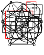
(b) SC₁-layout

Figure 1: Two 2-planar drawings of $K_{5}$.

The well-known algorithm of Biedl and Kant [6] draws any connected graph of maximum degree 4 orthogonally on a grid of size $n\times n$ with at most $2n+2$ bends, bending each edge at most twice (and, hence, yielding OC₃-layouts). For the output of their algorithm applied to $K_{5}$, see Fig. 1(a). Note that their approach introduces crossings to the produced drawing. For planar graphs, they describe how to obtain planar orthogonal drawings with at most two bends per edge, except possibly for one edge on the outer face.

So far, smooth orthogonal drawings have been studied nearly exclusively for planar graphs. Bekos et al. [4] showed how to compute an SC₁-layout for any maximum degree 4 graph, but their algorithm does not consider the embedding of the given graph. For a drawing of $K_{5}$ computed by their algorithm, see Fig. 1(b). Also, in the produced drawings, the number of crossings that an edge may have is not bounded. Bekos et al. also showed that, if one does not restrict vertex degrees, many planar graphs do not admit (planar) SC₁-layouts under the Kandinsky model, where the number of edges using the same port is unbounded. They proved, however, that all planar graphs of maximum degree 3 admit an SC₁-layout (under the usual port constraint). For the same class of graphs, Alam et al. [1] showed how to get a polynomial drawing area ($O(n^{2})\times O(n)$) when increasing the curve complexity to SC₂. Further, they showed that every planar graph of maximum degree 4 admits an SC₂-layout, but not every such graph admits an SC₁-layout where the vertices lie on a polynomial-sized grid. They also proved that every biconnected outerplane graph of maximum degree 4 admits an SC₁-layout (respecting the given embedding).

In this paper, we study orthogonal and smooth orthogonal layouts of non-planar graphs, in particular, 1-planar graphs. Recall that $k$-planar graphs are those graphs that admit a drawing in the plane where each edge has at most $k$ crossings. Our goal is to extend the well-established aesthetic criterion ‘curve complexity’ of (smooth) orthogonal drawings from planar to 1-planar graphs.

1-planar graphs, introduced by Ringel [17], probably form the most-studied class of the beyond-planar graphs, which extend the notion of planarity. There are recent surveys on both 1-planar graphs [14] and beyond-planar graphs [9]. Mostly, straight-line drawings have been studied for 1-planar graphs. While every planar graph has a planar straight-line drawing (due to Fáry’s theorem), this is not true for 1-planar graphs [11, 22]. For the 3-connected case, the statement holds except for at most one edge on the outer face [2]. Given a drawing of a 1-planar graph, one can decide in linear time whether it can be “straightened” [13].

An important subclass of 1-planar graphs are outer-1-planar graphs. These are the graphs that have a 1-planar drawing where every vertex lies on the outer (unbounded) face. They are planar graphs, can be recognized in linear time [12, 3], and can be drawn with straight-line edges and right-angle crossings [8].

We are specifically interested in 1-plane and outer-1-plane graphs, which are 1-planar and outer-1-planar graphs together with an embedding. Such an embedding determines the order of the edges around each vertex, but also which edges cross and in which order. By the layout of a 1-plane graph we mean that the layout respects the given embedding, without stating this again. In contrast, the layout of a 1-planar graph can have any 1-planar embedding.

Our contribution.

Previous results and our contribution on (smooth) orthogonal layouts are listed in Table 1. We present new layout algorithms for $1$-planar graphs in the orthogonal model (Section 3) and in the smooth orthogonal model (Section 4), achieving low curve complexity and preserving 1-planarity. We study 1-plane graphs as well as the special case of outer-1-plane graphs, where all vertices lie on the outer face. We conclude with some open problems; see Section 5.

In particular, we show that all 1-plane graphs admit OC₄-layouts (Theorem 3.2) and SC₃-layouts (Theorem 4.1). We also prove that all biconnected outer-1-plane graphs admit OC₃-layouts (Theorem 3.4) and SC₂-layouts (Theorem 4.3). Three out of these four results are worst-case optimal: There exist biconnected 1-plane graphs that do not admit an OC₃-layout (Theorem 3.1) and biconnected outer-1-plane graphs that do not admit OC₂-layouts (Theorem 3.3) and SC₁-layouts (Theorem 4.2).

Table 1: Comparison of our results to previous work. The model K(andinsky)-SC₁ does not restrict the number of edges per port to one. (^⋆) except for the octahedron (OC₄). “Super-poly” means that the drawings are not known to be of polynomial size.

		max.	curve	drawing
	graph class	deg.	complexity	area	reference
orthogonal	general	4	OC3	$n\times n$	[6]
	planar	4	OC3 (⋆)	$n\times n$	[6]
	1-plane	4	$\not\subseteq$ OC3 / OC4	$O(n)\times O(n)$	Thm. 3.1 / 3.2
	biconnected outer-1-plane	4	$\not\subseteq$ OC2 / OC3	$O(n)\times O(n)$	Thm. 3.3 / 3.4
smooth orthogonal	planar	4	SC2	super-poly	[1]
	planar, poly-area	4	$\not\supseteq$ SC1	—	[1]
	planar, OC2	4	$\not\subseteq$ SC1	—	[1]
	planar	3	SC2	$\lfloor{n^{2}}/4\rfloor\times\lfloor n/2\rfloor$	[1]
	planar	3	SC1	super-poly	[4]
	biconnected outerplane	4	SC1	super-poly	[1]
	general (non-planar)	4	SC1	$2n\times 2n$	[4]
	planar	$\infty$	$\not\subseteq$ K-SC1 / K-SC2	$O(n)\times O(n)$	[5, 4]
	biconnected 1-plane	4	SC3	$O(n)\times O(n^{2})$	Thm. 4.1
	biconnected outer-1-plane	4	$\not\subseteq$ SC1 / SC2	super-poly	Thm. 4.2 / 4.3

2 1-Planar Bar Visibility Representation

As an intermediate step towards orthogonal drawings, we introduce 1-planar bar visibility representations: Each vertex is represented as a horizontal segment – called bar – and each edge is represented as either a vertical segment or a polyline composed of a vertical segment and a horizontal segment between the bars of its adjacent vertices. Edges must not intersect other bars. If an edge has a horizontal segment, we call it red. The horizontal segment of a red edge must be on top of its vertical segment and crosses exactly one vertical segment of another edge – which is called blue. The vertical segment of a red edge must not be crossed; see Fig. 2. We consider every edge as a pair of two half-edges, one for each of its two endpoints. Red edges are split at their bend – the construction bend, such that each half-edge consists of either a vertical or a horizontal segment. Observe that horizontal half-edges are always red. We show that every 1-planar graph has a 1-planar bar visibility representation, following the approach of Brandenburg [7]:

For a 1-planar embedding, we define a kite to be a $K_{4}$ induced by the end vertices of two crossing edges with the property that each of the four triangles induced by the crossing point and one end vertex of each of the two crossing edges is a face. A crossing is caged if its end vertices induce a kite. Let now $G$ be a 1-planar graph. As a preprocessing step, $G$ is augmented to a not necessarily simple graph $G^{\prime}$, with the property that any crossing is caged and no planar edge can be added to $G^{\prime}$ without creating a new crossing or a double edge [2].

After the preprocessing step, all crossing edges are removed and a bar visibility representation for the produced plane graph $G_{p}$ is computed [19, 21]. To this end an $st$-ordering of a biconnected supergraph of $G_{p}$ is computed, i.e., an ordering $s=v_{0}$, $v_{1}$, $\ldots$, $v_{n-2}$, $v_{n-1}=t$ of the vertices such that each vertex except $s$ and $t$ is adjacent to both, a vertex with a greater and a lower index. The $st$-number is the index of a vertex. The y-coordinate of each bar is chosen to be the $st$-number of the respective vertex.

Faces of size four that correspond to the kites of $G$ have three possible configurations: left/right wing or diamond configuration. Fig. 2 shows the configurations and how to insert the crossing edges in order to obtain a 1-planar bar visibility representation of $G^{\prime}$. Removing the caging edges results in a 1-planar bar visibility representation of $G$.

(a) left wing

(b) right wing

(c) diamond

Figure 2: Different configurations for kites in a 1-planar bar visibility representation.

An edge is a left, right, top or bottom edge for a bar if it is attached to the respective side of that bar. Note that only red edges of $G$ can be left or right edges for exactly one of their endpoints (and top edge for their other endpoint). If a bar has no bottom (top) edges, it is a bottom (top) bar, respectively. Otherwise it is a middle bar. For a bottom (top) bar, consider the x-coordinates of the touching points of its edges. We define its leftmost and rightmost edge to be the edge with the smallest and largest x-coordinate, respectively. If such a bar has a left or right edge then, by the previous definition, this is its leftmost or rightmost edge, respectively. Note that by the construction of the bar visibility representation, each bar has at most one left and at most one right red edge.

3 Orthogonal 1-Planar Drawings

In this section, we examine orthogonal 1-planar drawings. In particular, we give a counterexample showing that not every biconnected 1-plane graph of maximum degree 4 admits an OC₃-layout. On the other hand, we prove that every 1-plane graph of maximum degree 4 admits an OC₄-layout that preserves the given embedding. For biconnected outer-1-plane graphs we achieve optimal curve complexity 3.

3.1 Orthogonal Drawings for General 1-Planar Graphs

Theorem 3.1

Not every biconnected $1$-plane graph of maximum degree $4$ admits an OC₃-layout. Moreover, there is a family of graphs requiring a linear number of edges of complexity at least $4$ in any OC₄-layout respecting the embedding.

Proof

Consider the 1-planar embedding of a $K_{5}$ as shown in Fig. 3(a). The outer face is a triangle $T$ and all vertices have their free ports in the interior of $T$. Hence, $T$ has at least $7$ bends, and at least one edge of $T$ has at least $3$ bends.

For another example refer to Fig. 3(b), where vertices $a$, $b$, and $c$ create a triangle with the same properties. We use $t$ copies of the graph of Fig. 3(b) in a column and glue them together by connecting the top and bottom gray vertices of consecutive copies with an edge, as well as the topmost vertex of the topmost copy and the bottommost vertex of the bottommost copy. The graph has $n=9t$ vertices and at least $t$ edges of complexity at least 4.

(a) $K_{5}$

(b) a 9-vertex graph

Figure 3: Biconnected 1-plane graphs without OC₃-layout

Figure 4: Octahedron

In order to achieve an OC₄-layout for 1-plane graphs, we will use a general property of orthogonal drawings of planar graphs: Consider two consecutive bends on an edge $e$ with an incident face $f$. We say that the pair of bends forms a U-shape if they are both convex or both concave in $f$ and an S-shape, otherwise. It follows from the flow model of Tamassia [20] that if a planar graph has an orthogonal drawing with an S-shape then it also has an orthogonal drawing with the identical sequence of bends on all edges except for the two bends of the S-shape that are removed. Thus, by planarization, any pair of S-shape bends can be removed as long as the two bends are not separated by crossings.

Theorem 3.2

Every $n$-vertex $1$-plane graph of maximum degree $4$ admits an OC₄-layout on a grid of size $O(n)\times O(n)$.

Proof

Let $G$ be a 1-planar graph of maximum degree 4 and consider a 1-planar bar visibility representation of $G$. If $G$ is not connected, we draw each connected component separately, therefore we assume that $G$ is connected.

Each vertex is placed on its bar. Figs. 5 and 6 indicate how to route the adjacent half-edges. Recall that the S-shape bend pairs can be eliminated. Thus, a horizontal half-edge gets at most one extra bend and a vertical half-edge gets at most two extra bends; see Fig. 6. We call a half-edge extreme if it was horizontal and got one bend or vertical and got two bends that create a U-shape.

(a)

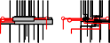
(b)

(c)

(d)

(e)

(f)

Figure 5: Replacing a middle bar with a vertex in the presence of (a)–(c) zero, (d)–(e) one, and (f) two horizontal half-edges

(a)

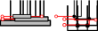
(b)

(c)

(d)

(e)

Figure 6: Replacing a bottom bar of degree $4$ with a vertex.

It suffices to show that the edges can be routed such that no edge is composed of two extreme half-edges. Even for red edges where we have the construction bend, we either get one extra bend from the horizontal (extreme) half-edge or two extra bends from the vertical (extreme) half-edge. Observe that an edge is extreme if and only if it is the rightmost or leftmost edge of a bottom or top bar, respectively, and it is attached to the bottom or top of the vertex, respectively. For each bottom or top bar we have the free choice to set either its rightmost or leftmost half-edge to become extreme. Consider the following bipartite graph $H$. The vertices of $H$ are the top and bottom bars, as well as their leftmost and rightmost edges. A bar-vertex and an edge-vertex are adjacent in $H$ if and only if the bar and the edge are incident. Observe that each bar-vertex has degree two and each edge-vertex has degree at most two, thus $H$ is a union of disjoint paths and cycles and there is a matching of $H$ in which each bar-vertex is matched. This matching defines the extreme half-edges. It assigns exactly one half-edge to every bottom or top-bar and matches at most one half-edge of each edge.

3.2 Orthogonal Drawings of Outer-1-Plane Graphs

Since outer-1-planar graphs are planar graphs [3], a planar orthogonal layout could be computed with curve complexity at most three. For example, in Fig. 7(a) we can see an outer-1-plane graph with a planar embedding in Fig. 7(b). Arguing similarly as we did for the proof of Theorem 3.1 it follows that there will be at least two bends on an edge of the outer face. In this particular case, Fig. 7(c) shows an outer-1-planar drawing of the same graph with at most two bends per edge. In the following we compute 1-planar orthogonal layouts for biconnected outer-1-planar graphs with optimal curve complexity three that also preserve the initial outer-1-planar embedding.

Theorem 3.3

Not every biconnected outer-$1$-plane graph of maximum degree $4$ admits an OC₂-layout.

(a) outer-1-planar embedding

(b) planar embedding

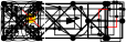
(c) OC₃-layout

Figure 7: An outer-1-plane graph.

(a) $K_{4}$

(b) two biconnected copies of $K_{4}$

Figure 8: Biconnected outer-1-plane graph that does not admit an OC₂-layout with the same embedding.

Proof

$K_{4}$ is a biconnected outer-1-plane graph. Actually, it has a unique OC₂-layout as shown in Fig. 8(a). When connecting two copies of $K_{4}$ by two intersecting edges as in Fig. 8(b), it is not possible to draw the resulting graph such that the connector edges intersect and have curve complexity two.

Theorem 3.4 ()

Every biconnected outer-$1$-plane graph of maximum degree $4$ admits an OC₃-layout in an $O(n)\times O(n)$ grid, where $n$ is the number of vertices.

Proof (sketch)

Let $G$ be an outer-1-planar graph of maximum degree 4. Observe that all crossings can be caged without changing the embedding: A maximal outer-1-planar graph always admits a straight-line outer-1-planar drawing in which all faces are convex [11, 8]. We would directly obtain the required curve complexity if there were no top or bottom bars of degree 4. Instead, our proof is based on a 1-planar bar visibility representation of $G$ produced by a specific $st$-ordering. Let $s$ and $t$ be two vertices on the outer face. Define $S_{l}$ and $S_{r}$ to be the sequences of vertices on the left path and on the right path from $s$ to $t$ along the outer face of $G$, respectively. We choose $s,S_{l},S_{r},t$ as our $st$-ordering. Observe that this is also an st-ordering of the caged and planarized graph $G_{p}$.

We process middle bars as in the algorithm of Theorem 3.2. For the top and bottom bars of degree 4 we choose differently which half-edge will be attached to the north or south port, respectively. Let $v$ be a vertex such that $b(v)$ is a top or bottom bar of degree 4. Let $e_{l}=(v,v_{l})$ and $e_{r}=(v,v_{r})$ be its leftmost and rightmost edge, respectively. Assume that $v\in S_{l}\cup\{s\}$ and $b(v)$ is a bottom bar. If $v_{l}\in S_{l}$, we choose edge $e_{l}$ to be attached to the south port of $v$, otherwise we choose edge $e_{r}$. If $b(v)$ is a top bar of degree 4 we choose its leftmost edge $e_{l}$ to be attached to the north port of $v$. Symmetrically, if $v\in S_{r}\cup\{t\}$ and $b(v)$ is a top bar, we choose $e_{r}$ for the north port of $v$ if $v_{r}\in S_{r}$, otherwise we choose $e_{l}$. If $b(v)$ is a bottom bar we choose its rightmost edge $e_{r}$ for the south port of $v$.

The above choice has the following property (detailed proof in Appendix 0.A): Any edge with three or four bends contains two consecutive bends that create an S-shape. The two bends are always connected with a vertical segment. If this is an uncrossed edge of $G$, the S-shape can be eliminated. For crossing edges, we prove that only one edge per crossing may have more than two bends. If the vertical segment connecting the two bends of the S-shape is crossed, we apply the flow technique of Tamassia [20] around the crossing point and reduce the number of bends (for details refer to Appendix 0.A).

4 Smooth Orthogonal 1-Planar Drawings

In this section we examine smooth orthogonal 1-planar drawings. In particular, we show that every 1-plane graph of maximum degree 4 admits an SC₃-layout that preserves the given embedding. For biconnected outer-1-plane graphs, we achieve SC₂, which is optimal for this graph class.

4.1 Smooth Orthogonal Drawings for General 1-Planar Graphs

(a)

(b)

(c)

Figure 9: Smoothing process of U-shapes created by top (bottom) bars.

Theorem 4.1

Every $1$-plane graph of maximum degree $4$ admits an SC₃-layout in $O(n)\times O(n^{2})$ area.

Proof

We compute an SC₃-layout based on an OC₄-layout computed by the algorithm of Theorem 3.2. Observe that in the OC₄-layouts calculated by our approach, the area bounded U-shaped half-edges created at top and bottom bars is vertex-free (see gray area in Fig. 9(a)), and, each vertex is located on a separate level. We replace one bend of each U-shaped half-edge by a dummy vertex; see Fig. 9(a). By doing so, we split each U-shaped half-edge into a vertical edge and an $L$-shaped half-edge. In the following, we treat the $L$-shaped half-edge as if the bend was on an $L$-shaped half-edge incident to the dummy vertex. We process $V=\{v_{1},v_{2},\ldots,v_{n}\}$ in the ascending vertical order of vertices (including dummy vertices). For $v_{i}$, let $\Delta^{\uparrow}_{i}$ be the largest horizontal distance between $v_{i}$ and any bend on incident $L$-shaped half-edges leading to neighbors with larger index. Let $\Delta^{\downarrow}_{i}$ be the corresponding value for bends at incident $L$-shaped half-edges and construction bends of red edges incident to edges leading to neighbors with smaller index. We increase the y-coordinate of all $v_{j}$ with $j\geq i$ by $\Delta^{\downarrow}_{i}$ units and then the y-coordinate of all $v_{k}$ with $k>i$ by $\Delta^{\uparrow}_{i}$ units. Bends on $L$-shaped half-edges and construction bends of red edges leading to neighbors with smaller index will be moved together with the corresponding vertex. Note that the region enclosed by U-shapes created at top and bottom bars remains empty; see Fig. 9(b). After the stretching, we remove the additional dummy vertices.

Each U-shaped half-edge will be replaced by a semi-circle which fits into the corresponding stretched empty region. We place the semi-circle directly incident to the endpoint which created the U-shape; see Fig. 9(c). Then we replace each intersected $S$-shaped half-edge formed by a construction bend of a red edge by two consecutive quarter arcs incident to the top endpoint of the edge. Recall that if a red edge has an $S$-shape from its top vertex, it has no bend from its bottom vertex. Further we replace each remaining bend by a quarter arc starting at the corresponding endpoint. Arcs at the two endpoints will be connected by a vertical segment. The correctness follows from the fact that the regions stretched to make space for drawing arcs were empty in the initial drawing.

The area of the resulting drawing is $O(n)\times O(n^{2})$ as the input drawing had $O(n)\times O(n)$ area and for every vertex the stretching operation increases the height by at most the length of the longest horizontal segment (i.e. $O(n)$).

4.2 Smooth Orthogonal Drawings for Outer-1-Plane Graphs

We focus on smooth layouts of outer-1-plane graphs. We demonstrate that curve complexity one is not always possible, but curve complexity two can be achieved for biconnected outer-1-plane graphs. We start with the following observation. The complete graph on four vertices with free ports towards its outer face has a unique SC₁-layout, shown in Fig. 10(a). Removing one edge and restricting all ports towards its outer face, there exist two SC₁-layouts, see Figs. 10(b) and 10(c).

(a)

(b)

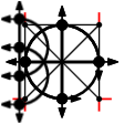
(c)

(d)

(e)

(f)

(g)

Figure 10: (a) SC₁-layouts for $K_{4}$ and (b)–(c) for $K_{4}-e$ with restricted ports. (d) A biconnected outer-1-plane graph that does not have an SC₁-layout. (e)-(g) SC₁-layouts of a subgraph of (d).

Theorem 4.2

Not every biconnected outer-$1$-plane graph of maximum degree $4$ has an SC₁-layout.

Proof

Take the graph in Fig. 10(d). It has two subgraphs isomorphic to $K_{4}-e$ (with restricted ports) that share a vertex. Combining two drawings for both copies gives rise to the three drawings in Figs. 10(e)–10(g) in which the edge between the two highlighted vertices cannot be added with curve complexity one.

To achieve SC₂-layouts for biconnected outer-1-plane graphs (see Fig. 12 for an example), we modify the algorithm of Alam et al. [1] for outerplane graphs; see Appendix 0.B for details.

Theorem 4.3 ()

Every biconnected outer-$1$-plane graph of maximum degree $4$ has an SC₂-layout. The drawing area may be super-polynomial.

Proof (sketch)

The algorithm of Alam et al. [1] processes the faces of the graph along the weak-dual, i.e., the dual graph omitting the outer face and rooted at some inner face. For the next face, one of its edges (the reference edge) is already drawn and imposes the drawing of the face. Figures 11(a)–11(f) show the different cases.

We define an auxiliary graph $G^{\prime}$: Let $G$ be a biconnected outer-1-plane graph, and let $G_{\mathrm{p}}$ be the planarized graph of $G$, where crossing points are replaced with dummy vertices. Three types of dummy vertices exist in $G_{\mathrm{p}}$: dummy-cuts (cut vertices), in-dummies (only incident to inner faces), and out-dummies. $G^{\prime}$ contains all in-dummy and out-dummy vertices of $G_{\mathrm{p}}$, while dummy-cuts are replaced by a caging cycle. The face inside a caging cycle is called a cut-face. All other faces are called normal. Faces are processed along a traversal of the weak dual of $G^{\prime}$. As $G^{\prime}$ may not be outerplanar, its weak dual does not have to be acyclic. It contains cycles of length four around in-dummies (see Fig. 11(m)). The auxiliary graph $G^{\prime}$ also contains virtual edges that are red. These are edges added for caging dummy-cuts and edges added to complete the process of faces around an in-dummy. Figures 11(g)–11(j) show how to process normal faces not appearing in Alam et al. [1]. When processing a cut-face, we draw the crossing edges instead of the caging cycles; see Figs. 11(k)–11(l) for two out of ten cases. Finally, in order to draw the fourth face around an in-dummy, we ensure that the edge-segments incident to the dummy vertex have the same length; see Fig. 11(n) for an example.

(a)

(b)

(c)

(d)

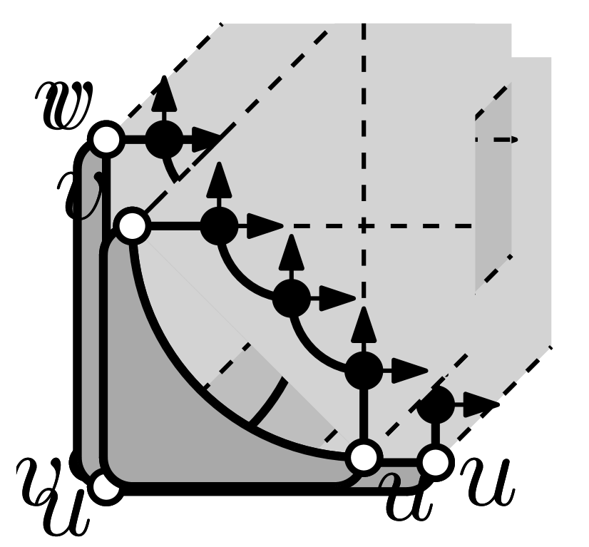
(e)

(f)

(g)

(h)

(i)

(j)

(k)

(l)

(m)

(n)

Figure 11: Constructing an SC₂-drawing of biconnected outer 1-planar graphs.

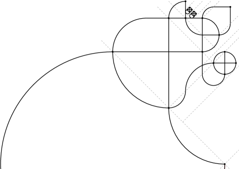
Figure 12: SC₂-layout of an outer-1-plane graph. Largest 3/4-arc only partially drawn.

5 A List of Open Problems

• Can we improve our curve complexity bounds if we restrict ourselves to more strongly connected classes of graphs (of maximum degree 4)?

• Candidate subclasses of outer-1-plane graphs for SC₁-layouts are for example outer-IC-plane graphs where crossings are independent. A possible variant would be to allow degenerate layouts where pairs of edges can touch but not cross.

• Is there a 1-plane graph that does not admit an SC₂-layout?

• Do biconnected outer-1-plane graphs admit an SC₂-layout with polynomial drawing area?

• Do similar results also hold for $2$-planar graphs and more generally beyond-planar graphs?

Appendix

Appendix 0.A Additional Material for Section 3.2

See 3.4

Proof

Let $G$ be an outer-1-planar graph of maximum degree 4. We want to use again a 1-planar bar visibility representation. First observe that all crossings in an outer-1-planar graph can be caged without changing the embedding: A maximal outer-1-planar graph always admits a straight-line outer-1-planar drawing in which all faces are convex [11, 8]. We would obtain the required curve complexity if there were no top or bottom bars of degree 4. Instead we will work with a specialized $st$-ordering.

Let $s$ and $t$ be two vertices on the outer face. Let $S_{l}$ and $S_{r}$ be the vertices on the left path and the right path from $s$ to $t$ along the outer face of $G$, respectively. Note that due to biconnectivity each vertex appears at most once in $S_{l}$ or $S_{r}$. We choose $s,S_{l},S_{r},t$ as the $st$-ordering for the construction of the 1-planar bar-visibility representation of $G$.

We want to replace every bar in a similar way as in the proof of Theorem 3.2. For the top and bottom bars of degree 4 we make a different choice based on which half-edge will be attached to the north or south port, respectively.

Let $v$ be a vertex such that $b(v)$ is a top or bottom bar of degree 4. Let $e_{l}=(v,v_{l})$ and $e_{r}=(v,v_{r})$ be its leftmost and rightmost edges, respectively. Assume first $v\in S_{l}\cup\{s\}$ and that $b(v)$ is a bottom bar. If $v_{l}\in S_{l}$, we select edge $e_{l}$ to be attached to the south port of $v$, otherwise we select edge $e_{r}$. If $b(v)$ is a top bar of degree 4, then all its neighbors appear before $v$ in the $st$-ordering and they belong to $S_{l}$, hence we choose its leftmost edge $e_{l}$ to be attached to the north port of $v$. Symmetrically, if $v\in S_{r}\cup\{t\}$ and $b(v)$ is a top bar, we choose $e_{r}$ for the north port of $v$ if $v_{r}\in S_{r}$, otherwise we choose $e_{l}$. And if $b(v)$ is a bottom bar, all its neighbors appear after $v$ and we choose its rightmost edge $e_{r}$ for the south port of $v$.

We claim that the above choice creates at most four bends, and in the case where three or four bends appear, two of them create an S-shape and are vertically aligned. Note that if the vertical segment connecting the two bends is not crossed, then the two bends can be eliminated and the theorem holds. So, consider an edge $e=(u,v)$ such that $u$ has a lower index than $v$. Three or more bends appear only if edge $e$ uses the south port of $u$ and/or the north port of $v$. There are three cases, depending on whether $u$, $v$ belong to $S_{l}\cup\{s\}$ or $S_{r}\cup\{t\}$.

Case 1: Suppose that $u,v\in S_{l}\cup\{s\}$. Assume first that $e$ uses the south port of $u$. Then $b(u)$ is a degree 4 bottom bar and $e$ is the leftmost edge of $b(u)$. All other neighbors of $u$ come after $v$ in the $st$-ordering. If there exists another edge attached to the bottom of $b(v)$ then this edge can only be incident to vertices with indices between $u$ and $v$, and therefore $e$ is the rightmost edge at the bottom of $b(v)$; refer to Fig. 13(a). When replacing $b(v)$ with vertex $v$, edge $e$ can only use the south or east port of $v$. This is true even in the case where $b(v)$ is a degree 4 top bar since in that case the north port will be used by the leftmost edge of $b(v)$ and not by $e$. There are three bends only if $e$ uses the east port of $v$ (see Fig. 13(b)). Two of them form an S-shape and are connected by a vertical segment as claimed.

Assume now that $e$ uses the north port of $v$. Then $b(v)$ is a degree 4 top bar and $e$ is the leftmost edge of $b(v)$. All other neighbors of $v$ come before $u$ in the $st$-ordering, and arguing similarly as before, we can conclude that $e$ cannot be the leftmost edge at the top of $b(u)$. Hence, $e$ will use either the north or the east port of $u$. Three bends are created only if $e$ uses the east port of $u$ (see Fig. 13(c)) and the claim holds.

Case 2: The case where $u,v\in S_{r}\cup\{t\}$ is similar to the case where $u,v\in S_{l}\cup\{s\}$ and is depicted in Figs. 13(d)-13(f).

Case 3: The last case that remains to consider for our claim, is the case where $u\in S_{l}\cup\{s\}$ and $v\in S_{r}\cup\{t\}$. Here, if $e$ uses the south port of $u$, then $b(u)$ is a degree 4 bottom bar and $e$ is its rightmost edge. It is not hard to see that $e$ is either the left edge of $b(v)$ or the leftmost edge attached to the bottom of $b(v)$. Therefore $e$ will not use the east port of $v$. Similarly, if $e$ uses the north port of $v$ then $e$ is the leftmost edge of the degree 4 top bar $b(v)$, and $e$ is the rightmost edge of the top of $b(u)$ and cannot use the west port of $u$. In any case, $e$ has at most four bends and satisfies the claim; refer to Figs. 13(g)-13(h) for the case where $e$ is drawn with four bends.

(a)

(b)

(c)

(d)

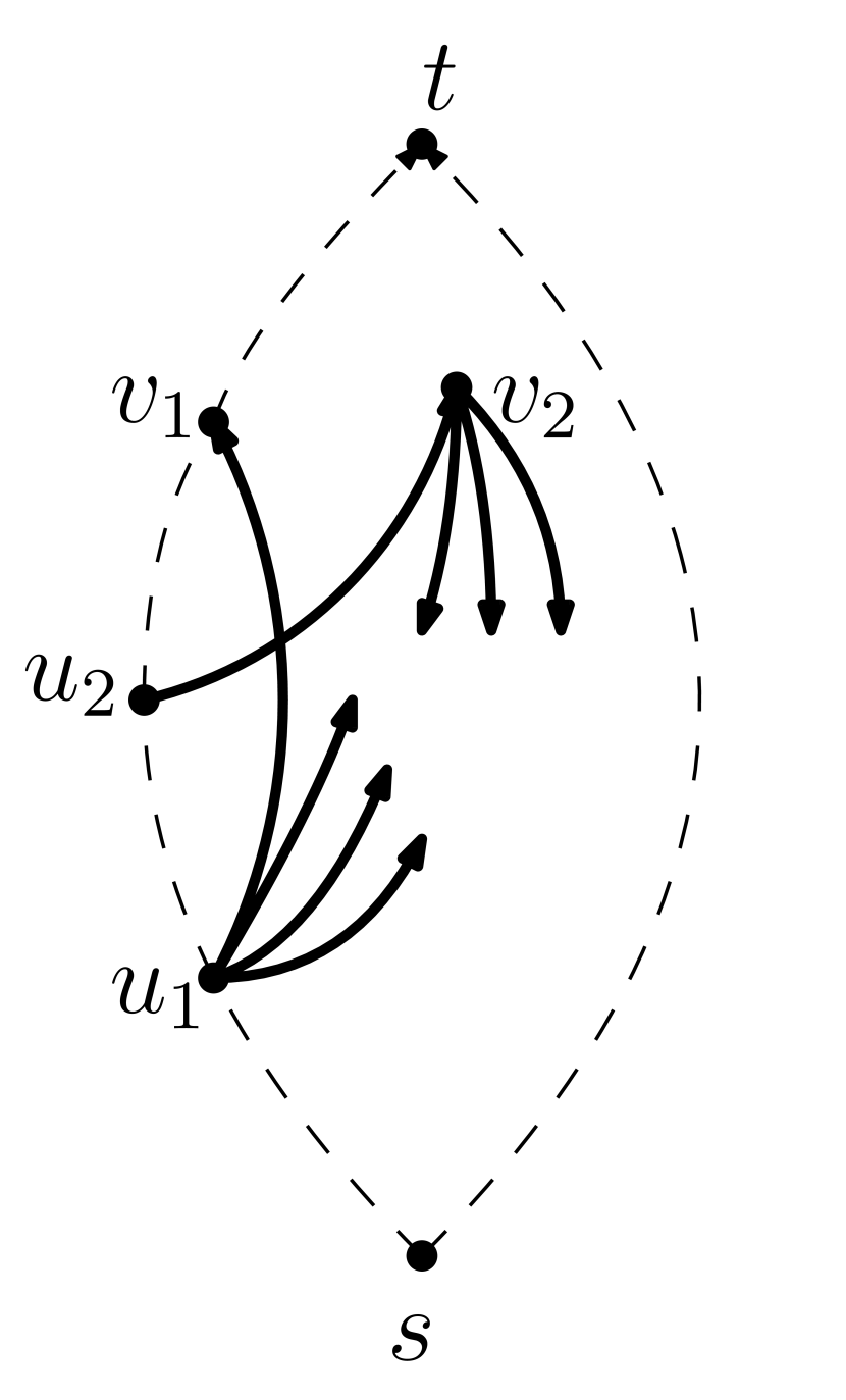
(e)

(f)

(g)

(h)

(i)

(j)

(k)

(l)

(m)

Figure 13: Cases considered in the proof of Theorem 3.4.

As already mentioned the above claim implies that if the vertical segment connecting the two bends of the S-shape is not crossed, then the S-shape can be eliminated so that the theorem holds. This is true if edge $e=(u,v)$ is a planar edge of $G$ or if it is a crossing red edge. It remains to consider blue edges. Recall that the selection of red and blue edges for the construction of the 1-planar bar visibility representation assured that the vertically drawn blue edge is always incident to the topmost bar. Let $e_{1}=(u_{1},v_{1})$ and $e_{2}=(u_{2},v_{2})$ be two crossing edges, such that $u_{1}$ appears before all other vertices in the $st$-ordering, and $u_{2}$ appears before $v_{2}$. We distinguish three cases depending on whether we have a diamond configuration, a left wing, or a right wing configuration in the 1-planar bar visibility representation.

• $e_{1}$ and $e_{2}$ create a diamond configuration. In this case we have $u_{1},u_{2}\in S_{l}\cup{\{s\}}$ and $v_{1},v_{2}\in S_{r}\cup{\{t\}}$ as shown in Fig. 13(i). Due to 1-planarity only edge $e_{2}$ can be drawn with three or four bends and this is always the red edge of a diamond configuration in the 1-planar bar visibility representation.

• $e_{1}$ and $e_{2}$ create a left wing configuration; refer to Fig. 13(j). In this case $e_{2}$ is the blue edge and vertices $u_{1},u_{2},v_{1}$ are in $S_{l}\cup{\{s\}}$. By outer-1-planarity, $b(u_{2})$, cannot have a top edge to the right of $e_{2}$ nor an additional edge to $S_{r}\cup t$. Thus, $e_{2}$ cannot be attached to the west or the south port of $u_{2}$. Hence, if $e_{2}$ has more than two bends, then $b(v_{2})$ must be a degree 4 top bar, $e_{2}$ uses the north port of $v_{2}$ and the east port of $u_{2}$. Figure 13(l) shows the drawing of the two crossing edges. Now consider the red edge $e_{1}$. By outer-1-planarity, $b(u_{1})$ cannot have a top edge to the right of $e_{1}$ nor an additional edge to $S_{r}\cup t$. Thus, $e_{1}$ cannot be attached to the west or the south port of $u_{1}$. Similarly, $e_{1}$ is not attached to the north or west port of $v_{1}$ and the construction bend of $e_{1}$ was not removed due to an S-shaped pair of bends. We apply the flow technique around the crossing point of $e_{1}$ and $e_{2}$ as indicated in Fig. 13(l): two bends of $e_{2}$ are removed and the construction bend of $e_{1}$ is moved to the other side of the crossing.

• The case where $e_{1}$ and $e_{2}$ create a right wing is symmetric to the previous case and indicated in Figs. 13(k) and 13(m).

We showed that whenever an edge has three or four bends, then two bends create an S-shape and are connected with a vertical segment. The two bends can be removed from the drawing giving an orthogonal 1-plane drawing with curve complexity three, as the theorem states.

Appendix 0.B Additional Material for Section 4.2

In order to achieve curve complexity two for smooth orthogonal drawings of biconnected outer-1-plane graphs, we modify the algorithm of Alam et al. [1] for outerplane graphs. Hence, in the following, we show how their SC₁-layout algorithm for outerplane graphs deals with biconnected outerplane graphs; for details we refer to the original paper [1].

In order to define an ordering of the faces, the algorithm of Alam et al. uses the weak dual tree $T$ of $G$ which is rooted at a leaf face. One edge of the root face incident to a degree two vertex and a vertex of degree at most three is selected as the first edge which will be drawn as a vertical segment. Following $T$ the graph is drawn face by face. Note that for each face that we draw, we have previously already drawn a single edge $(u,v)$ which will serve as a reference to select a suitable case from Fig. 14. Observe that in the cases shown in Figs. 14(a), 14(b), 14(d) and 14(e) a side-arc is introduced, that is, a convex quarter circle which will not serve as a new reference edge since it is incident to $u$ or $v$ which has remaining degree zero by construction.

(a)

(b)

(c)

(d)

(e)

(f)

Figure 14: Algorithm of Alam et al. [1] for SC₁-drawing outerplane graphs w.r.t. reference edge $(u,v)$: (a)–(c) inserting singletons and (d)–(f) inserting chains.

Planarity is proven as follows: When inserting a face above reference edge $(u,v)$, additionally a semi-strip $L_{u,v}$ bounded by rays of slope $+1$ emerging from $u$ and $v$ is introduced (lightgray in Fig. 14). Note that the two rays are not part of the lightgray semi-strip. If the face contains a side-arc an additional semi-strip touching the lightgray one is introduced (dark-gray in Fig. 14). This semi-strip has half the width of the lightgray one. The entire subgraph that can be separated by removing $u$ and $v$ will be located inside $L_{u,v}$ and, potentially, its two surrounding dark-gray semi-strips $L_{u,v}^{t}$ and $L_{u,v}^{b}$. In particular, let $(u^{\prime},v^{\prime})$ be the reference edge for the parent face in the weak dual $T$ that was used for placing $u$ and $v$. Then, all semi-strips defined by $u$ and $v$ will be contained in $L_{u^{\prime},v^{\prime}}$ and $L_{u^{\prime},v^{\prime}}^{t}$ (if it exists) and $L_{u^{\prime},v^{\prime}}^{b}$ (if it exists). Note that due to the number of ports available, if the subgraph incident to $u$ and $v$ uses $L_{u,v}^{t}$ or $L_{u,v}^{b}$, the corresponding edge neighboring $(u,v)$ cannot introduce another subgraph, hence no additional semi-strip is defined. Therefore, semi-strips can overlap only if they are defined by two faces, $f_{1}$ and $f_{2}$, such that $f_{1}$ is ancestor of $f_{2}$ in $T$, which prevents intersections.

Consider now a biconnected outer-1-planar graph $G$ and the planar graph $G_{\mathrm{p}}$ derived from $G$ by replacing all crossings with dummy vertices. In $G_{\mathrm{p}}$, there exist three types of dummy vertices: a dummy-cut, which is a cut vertex of $G_{\mathrm{p}}$ and its four edges belong to the outer face of $G_{\mathrm{p}}$, an out-dummy, which is not a cut vertex but is located on the outer face of $G_{\mathrm{p}}$ (has exactly two consecutive edges on the outer face), and an in-dummy, which is not on the outer face of $G_{\mathrm{p}}$.

See 4.3

Proof

We use a modified version of the algorithm of Alam et al. [1] which produces SC₁-layouts for outerplanar graphs without crossings. The algorithm requires an ordering of the vertices which is computed by the weak dual of a biconnected graph $G^{\prime}$ and an appropriate starting edge as reference for the first face. We first introduce a suitable order of the vertices which assumes that the first edge is selected appropriately.

Let $G$ be a biconnected outer-1-plane graph, and let $G_{\mathrm{p}}$ the planarized graph of $G$. We define a biconnected graph $G^{\prime}$ as follows. We keep all in-dummy and out-dummy vertices of $G_{\mathrm{p}}$ in $V(G^{\prime})$. For a dummy-cut $x$ created by a pair of crossing edges $(u,v)$ and $(u^{\prime},v^{\prime})$, we create a 4-wheel around $x$ by adding virtual edges as shown in Fig. 15(a) and remove $x$. Note that for each dummy-cut, we add at least two virtual edges that are on the outer face of $G^{\prime}$. Now $G^{\prime}$ is planar (not necessarily outerplanar), and contains only in-dummy vertices in its interior. If a face was created by a dummy-cut, we say it is a cut-face, otherwise it is a normal face. Let $e$ be the starting reference edge on the outer face of $G^{\prime}$ that is also incident to another face $f_{0}$. The weak dual of $G^{\prime}$ may contain cycles that are created by in-dummy vertices. However any cycle has length four and any two cycles are edge disjoint due to 1-planarity. We order the faces of $G^{\prime}$ by applying leftmost BFS on its weak dual and starting from $f_{0}$. Cycles of length four have two directed paths of the same length, say $f_{1},f_{2},f_{4}$ and $f_{1},f_{3},f_{4}$ where $f_{2}$ and $f_{3}$ are processed consecutively; see Fig. 15(b). We say that faces $f_{2}$ and $f_{3}$ create a facial pair. Note that faces $f_{1}$, $f_{2}$ and $f_{3}$ are normal faces. In order to process a face, we require that it has a reference edge. The only case where this edge may not be defined, is for a face $f_{4}$ of a cycle that is processed after facial-pair $f_{2}$ and $f_{3}$. In this case we add a virtual edge as shown in Fig. 15(b).

Consider a walk around the outer face of $G^{\prime}$. An edge $e$ might be a planar edge of $G$, or a half-edge (incident to an out-dummy) or it is an edge that does not belong to $G$ and was added for caging a dummy-cut. We claim that there exists at least one edge $e=(s,s^{\prime})$ that is either planar or a half-edge. Indeed, consider the planarized graph $G_{\mathrm{p}}$ derived from $G$ and a leaf-component $C$ of its BC-tree decomposition. If $C$ is the root-component then it clearly consists only of planar and half-edges. Otherwise, $C$ contains exactly one dummy-cut with degree two and at least two more vertices (the endpoints of the crossing edges of the dummy-cut). Since there are no other dummy-cuts and $C$ is biconnected, there exists a path between the two vertices that contains only planar edges and half-edges as claimed.

Let $e=(s,s^{\prime})$ be a planar or half-edge of $G^{\prime}$. We subdivide $e$ twice adding vertices $s_{1}$ and $s_{2}$. Then our reference edge for $G^{\prime}$ will be edge $(s_{1},s_{2})$ where both $s_{1}$ and $s_{2}$ have degree 2. We draw $(s_{1},s_{2})$ as a vertical segment and continue with the first face. Note that $s$ and $s^{\prime}$ are diagonally aligned and edge (or half-edge) $(s,s^{\prime})$ uses the west port of $s$ and south port of $s^{\prime}$. We replace the three segments used for $(s,s^{\prime})$ with a 3-quarter arc, i.e. with curve complexity one as shown in Fig. 16.

(a)

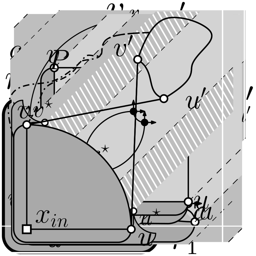
(b)

Figure 15: Introduction of virtual edges for dummy-cuts and in-dummies.

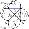
Figure 16: Starting the algorithm.   

In the following we describe how to draw $G$ based on the order defined on the faces of $G^{\prime}$. We proceed by adding one face of $G^{\prime}$ at a time. We make sure that virtual edges are not present in the final drawing and that when cut-faces are processed we draw the two crossing edges instead. Note that we deviate from the initial algorithm only if a face of $G^{\prime}$ contains either in-dummy vertices or is a cut-face. In order to process in-dummies, we may also use convex quarter-arcs as we shall shortly see. At each step, we use one curve per edge, except for three special cases where we use edges of complexity two: (i) the case of crossing edges that are drawn when processing a cut-face, (ii) planar edges of the outer face (which may be virtual) that cage in-dummy vertices, and (iii) planar edges of a triangular face (which may be virtual) with its reference edge drawn as a convex quarter arc.

Let $f$ be the next face to process. We distinguish three cases depending on whether $f$ is a normal face and does not belong to a facial-pair, is a normal face and belongs to a facial-pair, or is a cut-face. During the process we respect the following invariants:

1. If an edge is incident to an out-dummy, it is always drawn with curve complexity one, except for the case where it is a side-arc not incident to the north or east port of the out-dummy, where it may be drawn with curve complexity two.

2. If a virtual edge is a reference for a normal face, it is always drawn as a quarter-arc, either convex or concave, and its endpoints are diagonally aligned.

3. If the reference edge for a cut-face is non-virtual, then it is drawn with curve complexity one as a convex or concave quarter-arc, or as horizontal or vertical segment.

4. If a virtual side-arc is a reference for a cut-face, it is always drawn with curve complexity two.

The last invariant, namely I.4, implies that we need to alter the traditional drawing of Alam et al [1] in the cases where side-arcs are used. The corresponding drawings are given in Fig. 17.

(a)

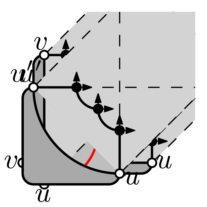
(b)

(c)

(d)

Figure 17: Using side-arcs with curve complexity two when (a)–(b) drawing singleton faces and (c)–(d) drawing chains. Red edges indicate virtual reference edges.

In addition to the invariants, we ensure that the following property holds throughout the process:

1. For an edge that is drawn as a convex quarter-arc, it holds that its two endpoints are not dummy vertices and have remaining degree at most one.

$f$ is a normal face and does not belong to a facial pair.

Suppose first that we encounter a normal face $f$ where the reference edge is a virtual edge $(u,v)$. By Invariant I.2 $(u,v)$ is drawn as a quarter-arc. We draw $f$ by replacing the virtual edge as demonstrated in Fig. 18(a) if $(u,v)$ is concave or as in Fig. 18(b) if it is convex. Note that all edges are drawn as quarter-arcs, horizontal or vertical segments. On the other hand, if the reference edge $(u,v)$ is not virtual, then the only case we need to pay extra attention is when $(u,v)$ is drawn as a convex quarter arc. If $f$ is a singleton we use the configuration of Fig. 18(c), where we draw the two edges with curve complexity two. If $f$ has more vertices, we use the placement of Figs. 18(d)–18(f), depending on whether the two side-arcs are virtual reference edges for cut-faces or not (hence, we preserve Invariants I.3 and I.4). Property P.1 and Invariant I.2 are satisfied since we do not use convex quarter-arcs and there are no virtual reference edges for normal faces. The only case that could violate Invariant I.1 is the case of adding a singleton face as in Fig. 18(c). However, the two vertices incident to the reference edge are not dummy vertices (by Property P.1). Also, after inserting the singleton face they have remaining degree zero, therefore, the third vertex cannot be an out-dummy either.

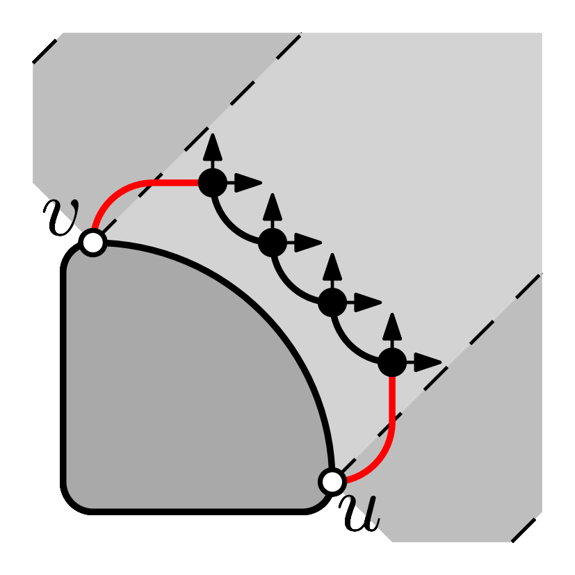
(a)

(b)

(c)

(d)

(e)

(f)

Figure 18: Processing a normal face whose reference edge is (a)–(b) virtual, and (c)–(f) non virtual.

$f$ is a normal face and belongs to a facial pair.

This case appears only when there is a cycle of four faces, say $f_{1},f_{2},f_{3},f_{4}$, with $x$ as their common in-dummy vertex. Face $f_{1}$ is a normal face and has already been drawn and $f$ is either $f_{2}$ or $f_{3}$. Since faces $f_{2}$ and $f_{3}$ are consecutive, we show how to draw them simultaneously, so that an appropriate reference edge can be defined for $f_{4}$ that will be drawn at a later step. Observe that $f_{2}$ and $f_{3}$ are normal faces and can be drawn as explained in the previous case. Let $(u,v)$ and $(u^{\prime},v^{\prime})$ be the two crossing edges of $G$, such that $f_{1}$ contains vertices $u$, $u^{\prime}$ and $x$, $f_{2}$ contains $x$, $u^{\prime}$ and $v$, and $f_{3}$ contains $x$, $u$ and $v^{\prime}$.

Also note that when $f_{1}$ is drawn, vertex $x$ has north and east ports available, so that edges $(x,v)$ and $(x,v^{\prime})$ are drawn as vertical and horizontal segments for $f_{2}$ and $f_{3}$ respectively. For edge $(v,v^{\prime})$ to become a reference edge for face $f_{4}$, we want vertices $v,v^{\prime}$ to be diagonally aligned (to preserve Invariant I.2). In order to do this we consider the following cases depending on the placement of vertices $u$, $x$, and $u^{\prime}$, as produced by the drawing of face $f_{1}$. Note that edges $(u,x)$ and $(x,u^{\prime})$ are always drawn with curve complexity one. Furthermore, they can be drawn neither as side-arcs of face $f_{1}$ (since they do not belong to the outer face), nor as convex quarter-arcs by Property P.1.

• Edges $(u,x)$ and $(x,u^{\prime})$ are drawn as consecutive concave quarter arcs (see Fig. 19(a)). Those arcs have the same size. Note that we are able to modify the sizes of the two arcs by moving $x$ along the diagonal $(u,u^{\prime})$ and without affecting the properties of the drawing. When moving $x$ from $u$ to $u^{\prime}$, the vertical segment used for $(x,v)$ increases and the horizontal segment for $(x,v^{\prime})$ decreases. Hence, we can find a placement for $x$ so that the two segments have same length; see Fig. 19(e).

• Edge $(u^{\prime},x)$ is drawn as horizontal segment and $(x,u)$ as a concave quarter arc (see Figs. 19(b) and  19(c)). In the case where the length of $(x,v)$ is smaller than the length of $(x,v^{\prime})$ (refer to Fig. 19(b)), we move $x$ towards $v^{\prime}$ and redraw $(x,u)$ with curve complexity two as shown in Fig. 19(f). The side-arc of $f_{2}$ is also redrawn with curve complexity two. In the other case, if the length of $(x,v)$ is greater than the length of $(x,v^{\prime})$ as in Fig. 19(c), we redraw $f_{2}$ by reducing the size of all new edges including $(x,v)$, and redrawing the side-arc of $f_{2}$ with curve complexity two. The corresponding drawing is shown in Fig. 19(g).

• The case of edge $(u^{\prime},x)$ drawn as concave quarter arc and $(x,u)$ as a vertical segment is symmetric to the previous one.

• Edge $(u^{\prime},x)$ is drawn as horizontal segment and $(x,u)$ as vertical segment (see Fig. 19(d)). We shorten the longer segment and redraw the side-edge of its face with edge complexity two as shown in Fig. 19(h).

Note that for the in-dummy vertex each incident half-edge is drawn with curve complexity one, except for the case shown in Fig. 19(f). In this special case, however, the corresponding crossing edges of $G$ are still of curve complexity two.

(a)

(b)

(c)

(d)

(e)

(f)

(g)

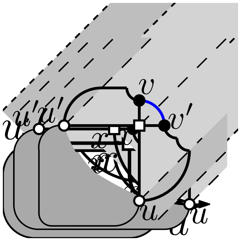
(h)

Figure 19: Drawing faces that belong to a facial pair. Blue edges may be virtual or non-virtual.

After aligning vertices $v$ and $v^{\prime}$ we draw reference edge $(v,v^{\prime})$ as a convex quarter arc; see Figs. 19(e)–19(h). It might be the case that this is a (virtual) reference edge, but then it satisfies Invariants I.2 and I.3. Since $v$ and $v^{\prime}$ are incident to dummy $x$, Property P.1 is preserved. We can argue that the remaining invariants are also satisfied in a similar way as we did in the case where $f$ did not belong to a facial pair. Invariant I.1 is maintained by the initial drawing of $f_{2}$ and $f_{3}$ as normal faces using the additional configurations of Fig. 17.

$f$ is a cut-face.

For any cut-face of $G^{\prime}$ there exist two virtual edges (see $(u,v^{\prime})$ and $(u^{\prime},v)$ in Fig. 15(a)) on the outer face of $G^{\prime}$ used solely for preserving biconnectivity. We ignore these two edges when processing $f$ and draw the pair of crossing edges $(u,v)$ and $(u^{\prime},v^{\prime})$ instead. We distinguish two cases, depending on whether edge $(u,u^{\prime})$ exists in $G$ or is a virtual edge. In the first case, we use one of the configurations shown in Fig. 20, depending on how $(u,u^{\prime})$ is drawn. Note, that $(u,u^{\prime})$ is not on the outer face of $G^{\prime}$, and therefore is not a side-arc of its face. For the other case, where $(u,u^{\prime})$ is a virtual edge, we use the configurations of Fig. 21 for all possible drawings of $(u,v)$. Observe, that if virtual edge $(u,u^{\prime})$ is a side-arc, it is drawn with curve complexity two by Invariant I.4. Since apart from crossing edges $(u,v)$ and $(u^{\prime},v^{\prime})$, we only add new reference edge $(v,v^{\prime})$ which is drawn as a concave quarter circle, we preserve Invariants I.1–I.4.

(a)

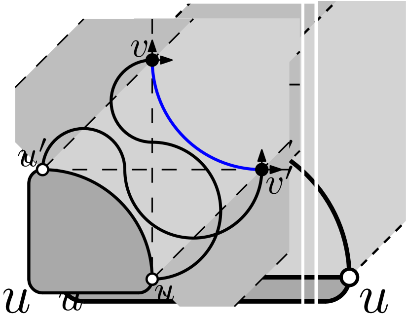
(b)

(c)

(d)

Figure 20: Drawing a cut-face where the reference edge $(u,v)$ exists and is drawn as (a) an horizontal segment, (b) a vertical segment, (c) a concave quarter-arc, or (d) a convex quarter-arc.

(a)

(b)

(c)

(d)

(e)

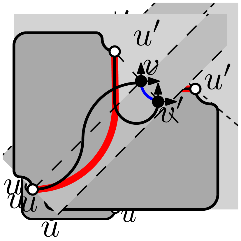
(f)

Figure 21: Drawing a cut-face where the reference edge $(u,v)$ is virtual and is drawn as (a) an horizontal segment, (b) a vertical segment, (c) a concave quarter-arc, (d) a convex quarter-arc. (e)–(f) a side edge.

Correctness.

The produced layout of $G^{\prime}$ is a smooth layout for our initial graph $G$, if we consider in-dummy and out-dummy vertices as crossing points. We claim that each edge has curve complexity at most two. This is true for all planar edges and crossing edges which create cut-faces. Also, crossing edges corresponding to in-dummies have edge complexity two as already claimed. The only case that remains to consider are crossing edges corresponding to out-dummies. Recall that by Invariant I.1 a half-edge incident to an out-dummy is drawn with curve complexity two only if it is a side-arc incident to either south or west port of the out-dummy. This case only occurs when processing facial pairs (refer to Fig. 19). Assume that half-edge $e$ is incident to the west port of out-dummy $x$. Then $e$ has a horizontal segment incident to $x$. To achieve edge complexity two for the crossing edge of $G$, we have to argue that the half-edge $e^{\prime}$ incident to $x$’s east port is drawn as a horizontal segment. By Invariant I.1, $e^{\prime}$ is drawn with edge complexity one, and by Property P.1, $e^{\prime}$ is not a convex quarter-arc. So, assume that $e^{\prime}$ was drawn as a side-arc. This implies that both $e$ and $e^{\prime}$ are on the outer face of $G^{\prime}$. A clear contradiction since an out-dummy has exactly two consecutive edges on the outer face. We conclude that $e^{\prime}$ has to be drawn as a horizontal segment. The case where $e$ is incident to the south-port is treated similarly.

To ensure that our construction preserves 1-planarity, we use a similar argument as in [1]. In particular, for every reference edge $(u,v)$, we define a diagonal semi-strip $L_{u,v}$ delimited by lines of slope $+1$ through $u$ and $v$; highlighted in light-gray in Figs. 17–21. Note that the two diagonal lines are not part of $L_{u,v}$. In addition, we may extend $L_{u,v}$ by two semi-strips $L_{u,v}^{t}$ and $L_{u,v}^{b}$ of $0.42$ times the width of $L_{u,v}$ surrounding $L_{u,v}$ from above and below, respectively; see dark-gray semi-strips in Figs. 17–21. However, we only extend $L_{u,v}$ if it is ensured that neighboring light-gray semi-strips are empty by the degree restriction (in particular, this is the case when the construction uses the north port of $v$ or east port of $u$, respectively). The drawing for the subgraph emerging from reference edge $(u,v)$ then is completely contained in $L_{u,v}$, $L_{u,v}^{t}$ (if it is introduced) and $L_{u,v}^{b}$ (if it is introduced). Observe that if a new reference edge $(u^{\prime},v^{\prime})$ is created in $L_{u,v}^{t}$ or $L_{u,v}^{b}$, we can choose a suitably small length of $(u^{\prime},v^{\prime})$ such that the entire subgraph emerging from $(u^{\prime},v^{\prime})$ remains inside $L_{u,v}^{t}$ or $L_{u,v}^{b}$. Also note that if we draw a cut-face with virtual reference edge $(u,u^{\prime})$ using one of the configurations of Figs. 21(a)–21(d), we restrict ourselves to a smaller semi-strip of width $0.16$ times the normal width of $L_{u,u^{\prime}}$ for drawing the component with reference edge $(v,v^{\prime})$ (not up to scale in the figures) so that dark gray semi-strips defined for $u$ or $u^{\prime}$ do not overlap $L_{u,u^{\prime}}$.

References

- [1] Alam, M.J., Bekos, M.A., Kaufmann, M., Kindermann, P., Kobourov, S.G., Wolff, A.: Smooth orthogonal drawings of planar graphs. In: Pardo, A., Viola, A. (eds.) Theoretical Informatics (LATIN’14). LNCS, vol. 8392, pp. 144–155. Springer (2014). https://doi.org/10.1007/978-3-642-54423-1_13
- [2] Alam, M.J., Brandenburg, F.J., Kobourov, S.G.: Straight-line grid drawings of 3-connected 1-planar graphs. In: Wismath, S.K., Wolff, A. (eds.) Graph Drawing (GD’13). LNCS, vol. 8242, pp. 83–94. Springer (2013). https://doi.org/10.1007/978-3-319-03841-4_8
- [3] Auer, C., Bachmaier, C., Brandenburg, F.J., Gleißner, A., Hanauer, K., Neuwirth, D., Reislhuber, J.: Outer 1-planar graphs. Algorithmica 74(4), 1293–1320 (2016). https://doi.org/10.1007/s00453-015-0002-1
- [4] Bekos, M.A., Gronemann, M., Pupyrev, S., Raftopoulou, C.N.: Perfect smooth orthogonal drawings. In: Bourbakis, N.G., Tsihrintzis, G.A., Virvou, M. (eds.) IISA. pp. 76–81. IEEE (2014). https://doi.org/10.1109/IISA.2014.6878731
- [5] Bekos, M.A., Kaufmann, M., Kobourov, S.G., Symvonis, A.: Smooth orthogonal layouts. J. Graph Algorithms Appl. 17(5), 575–595 (2013). https://doi.org/10.7155/jgaa.00305
- [6] Biedl, T., Kant, G.: A better heuristic for orthogonal graph drawings. Comput. Geom. Theory Appl. 9(3), 159–180 (1998). https://doi.org/10.1016/S0925-7721(97)00026-6
- [7] Brandenburg, F.J.: 1-visibility representations of 1-planar graphs. J. Graph Algorithms Appl. 18(3), 421–438 (2014). https://doi.org/10.7155/jgaa.00330
- [8] Dehkordi, H.R., Eades, P.: Every outer-1-plane graph has a right angle crossing drawing. Int. J. Comput. Geometry Appl. 22(6), 543–558 (2012). https://doi.org/10.1142/S021819591250015X
- [9] Didimo, W., Liotta, G., Montecchiani, F.: A survey on graph drawing beyond planarity. Arxiv report (2018), http://arxiv.org/abs/1804.07257
- [10] Duncan, C.A., Eppstein, D., Goodrich, M.T., Kobourov, S.G., Nöllenburg, M.: Lombardi drawings of graphs. J. Graph Algorithms Appl. 16(1), 85–108 (2012). https://doi.org/10.7155/jgaa.00251
- [11] Eggleton, R.B.: Rectilinear drawings of graphs. Utilitas Math. 29, 146–172 (1986)
- [12] Hong, S.H., Eades, P., Katoh, N., Liotta, G., Schweitzer, P., Suzuki, Y.: A linear-time algorithm for testing outer-1-planarity. Algorithmica 72(4), 1033–1054 (2015). https://doi.org/10.1007/s00453-014-9890-8
- [13] Hong, S.H., Eades, P., Liotta, G., Poon, S.H.: Fáry’s theorem for 1-planar graphs. In: Gudmundsson, J., Mestre, J., Viglas, T. (eds.) Computing and Combinatorics (COCOON’12). LNCS, vol. 7434, pp. 335–346. Springer (2012). https://doi.org/10.1007/978-3-642-32241-9_29
- [14] Kobourov, S.G., Liotta, G., Montecchiani, F.: An annotated bibliography on 1-planarity. Comput. Sci. Rev. 25, 49–67 (2017). https://doi.org/10.1016/j.cosrev.2017.06.002
- [15] Leighton, F.T.: New lower bound techniques for VLSI. Mathematical systems theory 17(1), 47–70 (1984). https://doi.org/10.1007/BF01744433
- [16] Leiserson, C.E.: Area-efficient graph layouts. In: Foundations of Computer Science (FOCS’80). pp. 270–281. IEEE (1980). https://doi.org/10.1109/SFCS.1980.13
- [17] Ringel, G.: Ein Sechsfarbenproblem auf der Kugel. Abh. Math. Seminar Univ. Hamburg 29(1–2), 107–117 (1965)
- [18] Roberts, M.J., Newton, E.J., Lagattolla, F.D., Hughes, S., Hasler, M.C.: Objective versus subjective measures of Paris metro map usability: Investigating traditional octolinear versus all-curves schematics. Int. J. Hum.-Comput. Stud. 71(3), 363–386 (2013). https://doi.org/10.1016/j.ijhcs.2012.09.004
- [19] Rosenstiehl, P., Tarjan, R.E.: Rectilinear planar layouts and bipolar orientations of planar graphs. Discrete & Computational Geometry 1, 343–353 (1986). https://doi.org/10.1007/BF02187706
- [20] Tamassia, R.: On embedding a graph in the grid with the minimum number of bends. SIAM J. Comput. 16(3), 421–444 (1987). https://doi.org/10.1137/0216030
- [21] Tamassia, R., Tollis, I.G.: A unified approach a visibility representation of planar graphs. Discrete & Computational Geometry 1, 321–341 (1986). https://doi.org/10.1007/BF02187705
- [22] Thomassen, C.: Rectilinear drawings of graphs. J. Graph Theory 12(3), 335–341 (1988). https://doi.org/10.1002/jgt.3190120306
- [23] Valiant, L.G.: Universality considerations in VLSI circuits. IEEE Trans. Comput. 30(2), 135–140 (1981). https://doi.org/10.1109/TC.1981.6312176