Preparing tunable Bell-diagonal states on a quantum computer

Abstract

The class of two-qubit Bell-diagonal states has been the workhorse for developing understanding about the geometry, dynamics, and applications of quantum resources. In this article, we present a quantum circuit for preparing Bell-diagonal states on a quantum computer in a tunable way. We implement this quantum circuit using the IBM Q 5 Yorktown quantum computer and, as an application example, we measure the non-local, steering, entanglement, and discord quantum correlations and non-local quantum coherence of Werner states.

Quantum properties such as coherence plenio , nonlocality Bell , steering Schrodinger , entanglement Werner , and discord Zurek have been identified as resources enabling the implementation of diverse quantum computation and communication protocols Shi ; Brunner ; Branciard ; Popescu ; Streltsov . The functions defined to quantify these quantum features based on the resource-theory framework plenio ; brito ; gallego ; vedral ; lloyd are frequently hard to compute analytically for general quantum states gharibian ; huang . Motivated by that observation, a subset of two-qubit states, the so called Bell-diagonal states (BDS), have been used extensively for better understanding some of these resources horodecki ; lang ; quan ; roszak ; meng ; kay ; wang ; singh ; maziero ; celeri ; castro ; paula ; luo ; hou ; han ; bromley ; bromley2 ; du ; auccaise ; auccaise2 ; aguilar .

So, due to its central place within the study of quantum resources, the experimental preparation of BDS is of apparent need. Recently Liu et al. showed how to prepare tunable Werner states in a linear optical system via the implementation of a depolarizing channel applied to a Bell state liu . Here we devise a simple quantum circuit that can be used to create tunable BDS on a quantum computer with the use of two auxiliary qubits. To exemplify the use of our protocol, we measure experimentally, using the IBM Q 5 Yorktown quantum computer ibm , the quantum nonlocality, steering, entanglement, discord, and non-local coherence of Werner states, which are a one-parameter subset of the BDS.

Our protocol can find application in verifying experimentally several theoretical results from the literature. For instance, one can apply our circuit to verify the relation between the sudden change phenomenon of quantum discord and the worst case fidelity in quantum teleportation, discovered in roszak . The necessity of quantum entanglement, instead of quantum non-locality, for better than classical fidelity of quantum teleportation exemplified using the thermal state associated with the magnetic dipolar interaction Hamiltonian castro can also be simulated using our protocol. This procedure can also be applied to verify the direct-dynamical entanglement-discord relations reported in feldman . Besides these three examples, one can easily find several other applications for our protocol, as e.g. in the experimental verification of the theoretical results reported in Refs. kay ; li ; han ; lang ; li2 .

The remainder of this article is organized as follows. We begin describing the class of BDS and presenting the quantum circuit we propose for its preparation on a quantum computer (QC). In the sequence we outline the implementation of this circuit on the IBM Q 5 Yorktown QC, hereafter referred to as ibmqx2. Then we present the experimental results we obtained for the quantum correlations and non-local coherence of Werner states. Finally, we report on a simple model that we have introduced to explain the noise influence on the experimental data and give our conclusions.

As the name indicates, two-qubit Bell-diagonal states read

$$\rho^{bd}=\sum_{j,k=0}^{1}p_{jk}|\beta_{jk}\rangle\langle\beta_{jk}|,$$ (1)

where $|\beta_{jk}\rangle=2^{-1/2}(|0\rangle\otimes|k\rangle+(-1)^{j}|1\rangle\otimes|k\oplus 1\rangle)$ are the Bell’s base states nilsen , with $\oplus$ being the modulo $2$ sum, $\{|j\rangle\}_{j=0}^{1}$ is the computational basis, and $p_{jk}$ is a probability distribution. This class of two-qubit states has the following four-qubit purification

$$|\tau\rangle_{abcd}=\sum_{j,k=0}^{1}\sqrt{p_{jk}}|j\rangle_{a}\otimes|k\rangle_{b}\otimes|\beta_{jk}\rangle_{cd}.$$ (2)

That is to say,

$$\rho^{bd}=\rho_{cd}=\mathrm{Tr}_{ab}(|\tau\rangle\langle\tau|_{abcd}),$$ (3)

with $\mathrm{Tr}_{ab}$ being the partial trace function mazieroPTr . Here we report that the quantum circuit shown in Fig. Preparing tunable Bell-diagonal states on a quantum computer generates the $4$-qubit state $|\tau\rangle_{abcd}$, and therefore that it can be used to prepare any BDS.

Figure 1: Quantum circuit we propose to generate tunable Bell-diagonal states on a quantum computer. The $R$ gates generate one-qubit superposition states. The CNOTs are used to copy the states of the qubits $a$ and $b$ to the qubits $c$ and $d$, respectively. By its turn, the Hadamard and the last CNOT gate are used for changing from the computational to the Bell basis. At the output, the joint state of qubits $c$ and $d$ is equivalent to $\rho^{bd}$ of Eq. (1) with $p_{jk}$ given as in Eq. (7).

In the circuit shown in Fig. Preparing tunable Bell-diagonal states on a quantum computer, we used the rotation

$$R(x)=\begin{bmatrix}\cos x&-\sin x\\ \sin x&\cos x\end{bmatrix},$$ (4)

the controlled-not gate

$$CNOT_{s\rightarrow s^{\prime}}=|0\rangle\langle 0|_{s}\otimes\sigma_{0}^{s^{\prime}}+|1\rangle\langle 1|_{s}\otimes\sigma_{1}^{s^{\prime}},$$ (5)

and the Hadamard gate

$$H=\frac{1}{\sqrt{2}}\begin{bmatrix}1&1\\ 1&-1\end{bmatrix}.$$ (6)

Above $\sigma_{0}^{s}\equiv\sigma_{0}$ is the $2\mathrm{x}2$ identity matrix and $\{\sigma_{j}^{s}\equiv\sigma_{j}\}_{j=1}^{3}$ are the Pauli matrices acting on qubit $s$ nilsen .

For the circuit in Fig. Preparing tunable Bell-diagonal states on a quantum computer, the relations among the probabilities in the BDS and rotation angles are seen to be

$$p_{jk}=\left(\cos^{2}\frac{\theta}{2}\right)^{1-j}\left(\sin^{2}\frac{\theta}{2}\right)^{j}\left(\cos^{2}\frac{\alpha}{2}\right)^{1-k}\left(\sin^{2}\frac{\alpha}{2}\right)^{k}.$$ (7)

For the calculation of quantum correlations, one usually start studying a maximally-mixed marginals state, $\rho_{3m}=2^{-2}(\sigma_{0}\otimes\sigma_{0}+\sum_{j,k=1}^{3}c_{jk}^{\prime}\sigma_{j}\otimes\sigma_{k})$, put to the normal form luo2 ,

$$\rho_{n}=2^{-2}\left(\sigma_{0}\otimes\sigma_{0}+\sum_{j=1}^{3}c_{jj}\sigma_{j}\otimes\sigma_{j}\right),$$ (8)

via local unitaries. The states $\rho_{n}$ are diagonal in the Bell basis, having the following eigenvalue–eigenvector pairs

$$\left(p_{jk}=\frac{1}{4}\left(1+(-1)^{j}c_{1}+(-1)^{j+k-1}c_{2}+(-1)^{k}c_{3}\right)\mbox{, }|\beta_{jk}\rangle\right),$$ (9)

where we used $c_{j}\equiv c_{jj}$.

Hence, from Eqs. (7) and (9) we see that given $\rho_{n}$, we can prepare any BDS in a tunable way by using as input to the quantum computer rotations $R(\theta/2)$ and $R(\alpha/2)$ the angles:

$$\theta = 2\arccos\sqrt{p_{00}+p_{01}}\mbox{,}$$ (10)

$$\alpha = 2\arccos\sqrt{p_{00}+p_{10}}.$$ (11)

For the implementation of the quantum circuit of Fig. Preparing tunable Bell-diagonal states on a quantum computer on the ibmqx2, we use $R(x/2)=U_{3}(x,0,0)$ with

$$U_{3}(\theta,\phi,\lambda)=\begin{bmatrix}\cos\frac{\theta}{2}&-e^{i\lambda}\sin\frac{\theta}{2}\\ e^{i\phi}\sin\frac{\theta}{2}&e^{i(\lambda+\phi)}\cos\frac{\theta}{2}\end{bmatrix}$$ (12)

being one of the ibmqx2 quantum gates ibm . The other gates we need are themselves directly included in the ibmqx2 set of ready-to-use quantum gates.

The experiments were carried out with the calibration parameters for the ibmqx2 shown in Table 1. We have chosen the following encoding (see Table 1) for implementation of the circuit in Fig. Preparing tunable Bell-diagonal states on a quantum computer:

$$a\rightarrow Q1\mbox{, }b\rightarrow Q3\mbox{, }c\rightarrow Q2\mbox{, }d\rightarrow Q4.$$ (13)

ibmqx2 parameters averages	Q0	Q1	Q2	Q3	Q4
Frequency (GHz)	5.29	5.23	5.02	5.29	5.08
T1 ($\mu$s)	50.81	59.80	64.93	56.37	56.81
T2 ($\mu$s)	45.89	39.70	63.14	31.60	32.32
Gate error ($10^{-3}$)	2.82	1.83	4.65	4.36	2.54
Readout error ($10^{-2}$)	4.16	1.89	1.93	2.87	4.61
MultiQubit gate error ($10^{-2}$)	$\stackrel{{\scriptstyle CX0\_1}}{{4.15}}$	$\stackrel{{\scriptstyle CX1\_2}}{{3.81}}$		$\stackrel{{\scriptstyle CX3\_2}}{{7.09}}$	$\stackrel{{\scriptstyle CX4\_2}}{{3.84}}$
	$\stackrel{{\scriptstyle CX0\_2}}{{4.42}}$			$\stackrel{{\scriptstyle CX3\_4}}{{5.28}}$

Table 1: Averages of the calibration data of the IBM Q 5 Yorktown quantum computer with which the experiments were performed. The temperature was $T=0.0159\text{ K}$.

With these settings, we prepared Werner states Werner ,

$$\rho_{w}=(1-w)\frac{\sigma_{0}\otimes\sigma_{0}}{4}+w|\beta_{11}\rangle\langle\beta_{11}|,$$ (14)

for eleven values of $w\in[0,1]$. We observe that $\rho_{w}$ is equivalent to $\rho_{n}$ if $c_{1}=c_{2}=c_{3}=-w$.

In order to experimentally reconstruct the prepared states, we consider general two-qubit states written in the form

$$\rho=\frac{1}{4}\sum_{j,k=0}^{3}c_{jk}\sigma_{j}\otimes\sigma_{k},$$ (15)

with $c_{jk}=\langle\sigma_{j}\otimes\sigma_{k}\rangle_{\rho}$. All of these averages can be obtained from the joint probability distributions of the local measurements of $\sigma_{j}$ and $\sigma_{k}$. Let

$$p_{j\pm,k\pm}:=\mathrm{Prob}(\sigma_{j}=\pm 1,\sigma_{k}=\pm 1).$$ (16)

Then, for $j,k=1,2,3$:

$$c_{jk}=p_{j+,k+}+p_{j-,k-}-p_{j+,k-}-p_{j-,k+}.$$ (17)

Using the marginal probability distributions

$$p_{j\pm}=p_{j\pm,k+}+p_{j\pm,k-}\mbox{ and }p_{k\pm}=p_{j+,k\pm}+p_{j-,k\pm}$$ (18)

we calculate

$$c_{j0}=p_{j+}-p_{j-}\mbox{ and }c_{0k}=p_{k+}-p_{k-}$$ (19)

for $j=1,2,3$ and for $k=1,2,3$. Finally, because $\mathrm{Tr}(\rho)=1$, we have $c_{00}=1$. Measurements of $\sigma_{3}$ are part of the ready-to-use operations of ibmqx2. To measure $\sigma_{1}$, we first applied the Hadamard gate $H$ and then measured $\sigma_{3}$. For measuring $\sigma_{2}$, we applied

$$S^{\dagger}=\begin{bmatrix}1&0\\ 0&-i\end{bmatrix},$$ (20)

then applied $H$, and finally measured $\sigma_{3}$. Above $\dagger$ denotes the transpose conjugate. With these measurement procedures, the probability distributions $p_{j\pm,k\pm}$ were estimated with $8192$ runs of the given quantum circuit and corresponding measurements. The computational basis representation of the reconstructed Werner states density matrices is shown in Fig. 2 for three values of $w$.

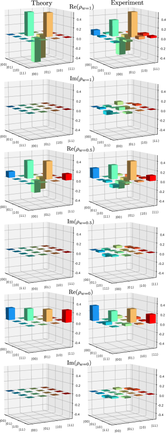
Figure 2: (color online) Computational basis representation of the real and imaginary parts of the theoretical-target and experimentally prepared density matrices corresponding to Werner states with three different values of the weight $w$.

In the sequence, we shall describe the quantumness measures we consider in this article. We begin by the $l_{1}$-norm coherence, with the standard basis used as the reference basis plenio :

$$C_{l_{1}}(\rho)=\sum_{j\neq k}|\langle j|\rho|k\rangle|$$ (21)

for $j,k=1,\cdots,d$ with $d$ being the dimension of the regarded state space. A natural candidate for quantifying the non-local extent of the quantum coherence of a bipartite system is pozzobom ; byrnes :

$$C(\rho)=C_{l_{1}}(\rho)-[C_{l_{1}}(\rho_{a})+C_{l_{1}}(\rho_{b})],$$ (22)

with the reduced states given by mazieroPTr : $\rho_{a}=\mathrm{Tr}_{b}(\rho)$ and $\rho_{b}=\mathrm{Tr}_{a}(\rho)$.

The quantum correlation (QC) named quantum discord is related to the minimal extent to which the correlations in a composite system are to be deprecated by local non-selective projective measurements. Here we use Ollivier-Zurek’s discord Zurek :

$$D(\rho)=I(\rho)-\max_{\Pi_{b}}I(\Pi_{b}(\rho)),$$ (23)

with the quantum mutual information being $I(x)=S(x_{a})+S(x_{b})-S(x)$, where $x_{a}$ and $x_{b}$ are reduced operators computed as mentioned above. By its turn, the measured state is defined as $\Pi_{b}(\rho)=\sum_{j}\sigma_{0}\otimes\Pi_{j}^{b}\rho\sigma_{0}\otimes\Pi_{j}^{b}$ with $\Pi_{j}^{b}\Pi_{k}^{b}=\delta_{j,k}\Pi_{j}^{b}$ and $\sum_{j}\Pi_{j}^{b}=\sigma_{0}$. We observe that once there is no known analytical formula for $D$ of general states (even for two qubits), the results we present in the sequence are obtained using numerical optimization.

Discord is known to be a weaker quantum correlation when compared to entanglement. This last type of quantum correlation, the non-separable correlations, are quantified here using the entanglement negativity vidal :

$$E(\rho)=||T_{p}(\rho)||_{tr}-1,$$ (24)

where $||X||_{tr}=\mathrm{Tr}\sqrt{X^{\dagger}X}$ is the trace norm and $T_{p}$ is the partial transposition operation mazieroPT .

For the two strongest forms of quantum correlations known, steering and non-locality, which cannot be explained using a local hidden state and a local hidden variable model, respectively, we use the formulas reported in costa . These authors considered measures for these quantities given by the maximum extend to which a given related inequality chsh ; horodecki2 ; ecavalcanti is violated. For deriving their analytical formulas, they used the standard form for two-qubit states luo2 :

$$4\rho=\sigma_{0}\otimes\sigma_{0}+\vec{a}\cdot\vec{\sigma}\otimes\sigma_{0}+\sigma_{0}\otimes\vec{b}\cdot\vec{\sigma}+\sum_{j=1}^{3}c_{j}\sigma_{j}\otimes\sigma_{j}.$$ (25)

This form can be obtained via local unitary transformations applied locally to a general two-qubit state, i.e., $\rho=U_{a}\otimes U_{b}\rho_{g}U_{a}^{\dagger}\otimes U_{b}^{\dagger}$, for $U_{a}U_{a}^{\dagger}=U_{a}^{\dagger}U_{a}=U_{b}U_{b}^{\dagger}=U_{b}^{\dagger}U_{b}=\mathbb{I}$, with

$$4\rho_{g}=\sigma_{0}\otimes\sigma_{0}+\vec{x}\cdot\vec{\sigma}\otimes\sigma_{0}+\sigma_{0}\otimes\vec{y}\cdot\vec{\sigma}+\sum_{j,k=1}^{3}c_{jk}\sigma_{j}\otimes\sigma_{k},$$ (26)

where $\vec{a}=O_{a}\vec{x}$, $\vec{b}=O_{b}\vec{y}$, and $\mathrm{diag}(c_{1},c_{2},c_{3})=O_{a}CO_{b}^{T}$, with $C=(c_{jk})$ being the correlation matrix and $O_{a}$ and $O_{b}$ are orthonormal matrices, i.e., $O_{a}O_{a}^{T}=O_{a}^{T}O_{a}=O_{b}O_{b}^{T}=O_{b}^{T}O_{b}=\mathbb{I}$ for $x^{T}$ denoting the transpose of the matrix $x$. The authors of costa obtained analytically the steering for three measurements per qubit,

$$S(\rho)=\max\left(0,\frac{||\vec{c}||-1}{\sqrt{3}-1}\right),$$ (27)

and the quantum non-locality for two measurements per qubit,

$$N(\rho)=\max\left(0,\frac{\sqrt{||\vec{c}||^{2}-c_{\min}^{2}}-1}{\sqrt{2}-1}\right),$$ (28)

with $c_{\min}$ being the minimum value among the components of the correlation vector $\vec{c}=(c_{1},c_{2},c_{3})$. Here we use as the correlation vector the singular values of the correlation matrix $C=(c_{jk})$, for $j,k=1,2,3$. We emphasize that the standard form is obtained via local unitary transformations, which do not affect the non-locality and steering functions above. Besides, we utilize the original state (reconstructed or theoretical) for the calculation of non-local coherence, discord, and entanglement.

The results for the state preparation fidelity and for all these quantum non-local coherence and correlation measures are presented in Fig. 3. The code we used to compute these functions is freely available at https://github.com/jonasmaziero/libPyQ.

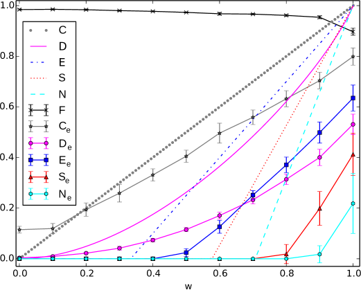
Figure 3: (color online) The x-like black points show the preparation fidelities, $F(\rho_{w},\rho_{w}^{exp})=Tr\sqrt{\sqrt{\rho_{w}}\rho_{w}^{exp}\sqrt{\rho_{w}}}$. The fidelity and the functions indicated in the legend by the subscript $e$ refer to averages, and the associated standard deviations, computed for the experimentally prepared states using seven rounds of experiments. $C$ stands for non-local coherence, shown in gray. In magenta is plotted the Ollivier-Zurek discord $D$. The entanglement negativity $E$ is shown in blue. The steering $S$ was given the color red and the non-locality $N$ is shown in cyan.

Even though the preparation fidelities shown in Fig. 3 have, in general, values quite close to the maximum value $1$, we see in this figure that the environmental noise and the quantum computer imperfections have significant detrimental effects on the quantum properties of the prepared states. This fact indicates that state preparation fidelity is not a reliable figure of merit if ones main purpose is the production and utilization of quantum correlations. For a related discussion, see Ref. mandarino .

It is interesting noticing that not only are the different quantum resources affected unevenly by those external influences, but the stronger the quantum correlation is, the more it is impacted. This fact can be qualitatively well explained in a simplified manner through the application of the composition of the amplitude damping and phase damping channels nilsen ; soares-pinto to one of the qubits of the theoretical-target Werner states:

$$\rho_{w}^{d}(a,p)=\sum_{j=0}^{2}K_{j}(a,p)\otimes\sigma_{0}\rho_{w}K_{j}^{\dagger}(a,p)\otimes\sigma_{0},$$ (29)

with the Kraus’ operators given by:

$$K_{0}(a,p) = \sqrt{p(1-a)}|1\rangle\langle 1|,$$ (30)

$$K_{1}(a,p) = \sqrt{a}|0\rangle\langle 1|,$$ (31)

$$K_{2}(a,p) = |0\rangle\langle 0|+\sqrt{(1-p)(1-a)}|1\rangle\langle 1|.$$ (32)

The quantum non-local coherence and correlations of $\rho_{w}^{d}(0.25,0.25)$ and of $\rho_{w}^{d}(0.15,0.15)$ are shown in Fig. 4.

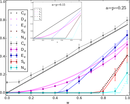
Figure 4: (color online) Quantum non-local coherence and quantum correlations of Werner states with one of the qubits evolved under the composition of phase damping and amplitude damping channels. Here we used the same labeling of Fig. 3, with the subscripts $d$ and $e$ standing for the function calculated using the decohered states of Eq. (29) and the experimental-reconstructed states, respectively. The main figure is for $a=p=0.25$ and in the inset are shown the corresponding curves for $a=p=0.15$. We see that, for $p=a=0.25$, although non-local coherence and correlations are under-estimated while discord, entanglement, and steering are over-estimated by the theoretical noise model, this model reproduces fairly well the experimentally observed greater susceptibility of stronger correlations to environmental interactions.

The results in Fig. 4 show that our simplified model of Eq. (29) describes well the main qualitative features of the experimental data. Besides, we see in the inset of Fig. 4 that by lowering the values of the amplitude and phase noise rates, one could significantly increase the values of the quantumness functions of the generated states.

In conclusion, in this article we gave a quantum circuit that can be used to prepare tunable Bell-diagonal states with a quantum computer. We implemented this quantum circuit using the IBM Q 5 Yorktown quantum computer and measured the non-local quantum coherence and discord, entanglement, steering, and non-local quantum correlations of experimentally reconstructed Werner states. Even though the noise and imperfections of the hardware utilized had a quite strong detrimental effect on the measured quantum correlations, we succeeded in verifying a hierarchy relation for quantum resources (see e.g. Ref. costa ) of the produced states: $N\Rightarrow S\Rightarrow E\Rightarrow D.$ The simple zero-temperature composite noise model we made to explain the obtained experimental results indicates that access to quantum computers with lower noise rates will allow for the application of our quantum circuit to produce even the strongest kinds of quantum correlation and also to test several interesting theoretical results that have been reported in the recent quantum information science literature using Bell-diagonal states.

- (1) T. Baumgratz, M. Cramer, and M. B. Plenio, Quantifying Coherence, Phys. Rev. Lett. 113, 140401 (2014).
- (2) J. S. Bell, On the Problem of Hidden Variables in Quantum Mechanics, Rev. Mod. Phys. 38, 447 (1966).
- (3) E. Schrödinger, Discussion of Probability Relations between Separated Systems, Math. Proc. Cambridge Phil. Soc. 31, 555 (1935).
- (4) R. F. Werner, Quantum states with Einstein-Podolsky-Rosen correlations admitting a hidden-variable model, Phys. Rev. A 40, 4277 (1989).
- (5) H. Ollivier and W. H. Zurek, Quantum Discord: A Measure of the Quantumness of Correlations, Phys. Rev. Lett. 88, 017901 (2001).
- (6) H.-L. Shi, S.-Y. Liu, X.-H. Wang, W.-L. Yang, Z.-Y. Yang, and H. Fan, Coherence depletion in the Grover quantum search algorithm, Phys. Rev. A 95, 032307 (2017).
- (7) N. Brunner, D. Cavalcanti, S. Pironio, V. Scarani, and S. Wehner, Bell nonlocality, Rev. Mod. Phys. 86, 419 (2014).
- (8) C. Branciard, E. G. Cavalcanti, S. P. Walborn, V. Scarani, and H. M. Wiseman, One-sided Device-Independent Quantum Key Distribution: Security, feasibility, and the connection with steering, Phys. Rev. A 85, 010301(R) (2012).
- (9) S. Popescu, Bell’s inequalities versus teleportation: What is nonlocality?, Phys. Rev. Lett. 72, 797 (1994).
- (10) A. Streltsov and H. Kampermann and D. Bruß, in Lectures on General Quantum Correlations and their Applications, edited by F. F. Fanchini, D. O. Soares-Pinto, and G. Adesso (Springer International Publishing, 2017) pp. 217-230.
- (11) S. G. A. Brito, B. Amaral, and R. Chaves, Noncontextual wirings, Phys. Rev. A 97, 022111 (2018).
- (12) R. Gallego and L. Aolita, The resource theory of steering, Phys. Rev. X 5, 041008 (2015).
- (13) V. Vedral, M. B. Plenio, M. A. Rippin, and P. L. Knight, Quantifying Entanglement, Phys. Rev. Lett. 78, 2275 (1997).
- (14) Z.-W. Liu, X. Hu, and S. Lloyd, Resource Destroying Maps, Phys. Rev. Lett. 118, 060502 (2017).
- (15) S. Gharibian, Strong NP-Hardness of the Quantum Separability Problem, Quantum Inf. Comp. 10, 343 (2010).
- (16) Y. Huang, Computing quantum discord is NP-complete, New J. Phys. 16, 033027 (2014).
- (17) R. Horodecki and M. Horodecki, Information-theoretic aspects of quantum inseparability of mixed states, Phys. Rev. A 54, 1838 (1996).
- (18) M. D. Lang and C. M. Caves, Quantum Discord and the Geometry of Bell-Diagonal States, Phys. Rev. Lett. 105, 150501 (2010).
- (19) Q. Quan, H. Zhu, S.-Y. Liu, S.-M. Fei, H. Fan, and W.-L. Yang, Steering Bell-diagonal states, Sci. Rep. 6, 22025 (2016).
- (20) K. Roszak and Ł. Cywiński, The relation between the quantum discord and quantum teleportation: the physical interpretation of the transition point between different quantum discord decay regimes, EPL 112, 10002 (2015).
- (21) Q. Meng, L. Yan-Biao, W. Xiao, and B. Zhong, The decoherence of quantum entanglement and teleportation in Bell-diagonal states, Chin. Phys. C 36, 307 (2012).
- (22) A. Kay, Using Separable Bell-Diagonal States to Distribute Entanglement, Phys. Rev. Lett. 109, 080503 (2012).
- (23) Y.-K. Wang, T. Ma, H. Fan, S.-M. Fei, and Z.-X. Wang, Super-quantum correlation and geometry for Bell-diagonal states with weak measurements, Quantum Inf. Proc. 13, 283 (2014).
- (24) H. Singh, Arvind, and K. Dorai, Experimentally freezing quantum discord in a dephasing environment using dynamical decoupling, EPL 118, 50001 (2017).
- (25) J. Maziero, L. C. Céleri, R. M. Serra, and V. Vedral, Classical and quantum correlations under decoherence, Phys. Rev. A 80, 044102 (2009).
- (26) L. C. Céleri and J. Maziero, in Lectures on General Quantum Correlations and their Applications, edited by F. F. Fanchini, D. O. Soares-Pinto, and G. Adesso (Springer International Publishing, 2017) pp. 309-337.
- (27) C. S. Castro, O. S. Duarte, D. P. Pires, D. O. Soares-Pinto, and M. S. Reis, Thermal entanglement and teleportation in a dipolar interacting system, Phys. Lett. A 380, 1571 (2016).
- (28) F. M. Paula, A. Saguia, T. R. de Oliveira, and M. S. Sarandy, Overcoming ambiguities in classical and quantum correlation measures, EPL 108, 10003 (2014).
- (29) S. Luo and Q. Zhang, Observable Correlations in Two-Qubit States, J. Stat. Phys. 136, 165 (2009).
- (30) J.-X. Hou, Y.-L. Su, S.-Y. Liu, X.-H. Wang, and W.-L. Yang, Geometric structure of quantum resources for Bell-diagonal states, Quantum Inf. Process. 17, 184 (2018).
- (31) W. Han, K.-X. Jiang, Y.-J. Zhang, and Y.-J. Xia, Quantum speed limits for Bell-diagonal states, Chin. Phys. B 24, 120304 (2015).
- (32) T. R. Bromley, M. Cianciaruso, and G. Adesso, Frozen Quantum Coherence, Phys. Rev. Lett. 114, 210401 (2015).
- (33) T. R. Bromley, M. Cianciaruso, R. L. Franco, and G. Adesso, Unifying approach to the quantification of bipartite correlations by Bures distance, J. Phys. A: Math. Theor. 47, 405302 (2014).
- (34) M.-M. Du, D. Wang, and L. Ye, The dynamic behaviors of complementary correlations under decoherence channels, Sci. Rep. 7, 40934 (2017).
- (35) R. Auccaise, L. C. Céleri, D. O. Soares-Pinto, E. R. deAzevedo, J. Maziero, A. M. Souza, T. J. Bonagamba, R. S. Sarthour, I. S. Oliveira, and R. M. Serra, Environment-Induced Sudden Transition in Quantum Discord Dynamics, Phys. Rev. Lett. 107, 140403 (2011).
- (36) R. Auccaise, J. Maziero, L. C. Céleri, D. O. Soares-Pinto, E. R. deAzevedo, T. J. Bonagamba, R. S. Sarthour, I. S. Oliveira, and R. M. Serra, Experimentally Witnessing the Quantumness of Correlations, Phys. Rev. Lett. 107, 070501 (2011).
- (37) G. H. Aguilar, O. J. Farías, J. Maziero, R. M. Serra, P. H. S. Ribeiro, and S. P. Walborn, Experimental Estimate of a Classicality Witness via a Single Measurement, Phys. Rev. Lett. 108, 063601 (2012).
- (38) T.-J. Liu, C.-Y. Wang, J. Li, and Q. Wang, Experimental preparation of an arbitrary tunable Werner state, EPL 119, 14002 (2017).
- (39) IBM Quantum Experience, http://www.research.ibm.com/ibm-q.
- (40) V. Feldman, J. Maziero, and A. Auyuanet, Direct-dynamical Entanglement-Discord relations, Quantum Inf. Process. 16, 128 (2017).
- (41) Z.-N. Li, J.-S. Jin, and C.-S. Yu, Probing Bell Diagonal State without Disturbing Its Correlations, Commun. Theor. Phys. 58, 47 (2012).
- (42) J. Li, C.-Y. Wang, T.-J. Liu, and Q. Wang, Experimental verification of steerability via geometric Bell-like inequalities, Phys. Rev. A 97, 032107 (2018).
- (43) M. A. Nielsen and I. L. Chuang, Quantum Computation and Quantum Information (Cambridge University Press, Cambridge, 2000).
- (44) J. Maziero, Computing partial traces and reduced density matrices, Int. J. Mod. Phys. C 28, 1750005 (2016).
- (45) S. Luo, Quantum discord for two-qubit systems, Phys. Rev. A 77, 042303 (2008).
- (46) M. B. Pozzobom and J. Maziero, Environment-induced quantum coherence spreading of a qubit, Ann. Phys. 377, 243 (2017).
- (47) C. Radhakrishnan, M. Parthasarathy, S. Jambulingam, and T. Byrnes, Distribution of Quantum Coherence in Multipartite Systems, Phys. Rev. Lett. 116, 150504 (2016).
- (48) G. Vidal and R. F. Werner, A computable measure of entanglement, Phys. Rev. A 65, 032314 (2002).
- (49) J. Maziero, Computing Partial Transposes and Related Entanglement Functions, Braz. J. Phys. 46, 605 (2016).
- (50) A. C. S. Costa and R. M. Angelo, Quantification of Einstein-Podolski-Rosen steering for two-qubit states, Phys. Rev. A 93, 020103 (2016).
- (51) J. F. Clauser, M. A. Horne, A. Shimony, and R. A. Holt, Proposed experiment to test local hidden-variable theories, Phys. Rev. Lett. 23, 880 (1969).
- (52) R. Horodecki, P. Horodecki, and M. Horodecki, Violating Bell inequality by mixed spin-12 states: necessary and sufficient condition, Phys. Lett. A 200, 340 (1995).
- (53) E. G. Cavalcanti, C. J. Foster, M. Fuwa, and H. M. Wiseman, Analog of the Clauser-Horne-Shimony-Holt inequality for steering, J. Opt. Soc. Am. B 32, A74 (2015).
- (54) A. Mandarino, M. Bina, C. Porto, S. Cialdi, S. Olivares, and M. G. A. Paris, Assessing the significance of fidelity as a figure of merit in quantum state reconstruction of discrete and continuous variable systems, Phys. Rev. A 93, 062118 (2016).
- (55) D. O. Soares-Pinto, M. H. Y. Moussa, J. Maziero, E. R. deAzevedo, T. J. Bonagamba, R. M. Serra, and L. C. Céleri, Equivalence between Redfield- and master-equation approaches for a time-dependent quantum system and coherence control, Phys. Rev. A 83, 062336 (2011).