1 Introduction

In standard single field inflation, the linearised dynamics of the scalar curvature fluctuation ${\cal R}$ is described by a quadratic action [1]

$$S_{R}\,=\,\int d\eta\,d^{3}x\,\frac{z_{S}^{2}}{2}\,\left[{\cal R^{\prime}}^{2}-(\vec{\nabla}{\cal R})^{2}\right]$$ (1)

with:

$$z_{S}\,\equiv\,a\,\frac{\dot{\phi}}{H},$$ (2)

where $\phi$ is the homogeneous scalar field profile, and prime and dot indicate respectively derivatives along conformal and physical time. The combination $z_{S}$ is known as the scalar pump field. If $z_{S}$ is an increasing function of time – as in a slow-roll regime, where the Hubble parameter and $\dot{\phi}$ are approximately constant – then inflation is in an attractor phase, ${\cal R}$ is conserved at superhorizon scales and its spectrum is almost scale invariant. However, if $z_{S}$ is rapidly decreasing for a brief interval, then the inflationary evolution is no longer an attractor: the would-be decaying mode of the curvature perturbation becomes dominant, and the power spectrum of modes leaving the horizon during this non-attractor phase can be enhanced by several orders of magnitude in a short time interval. This can occur for example in models where the scalar derivative rapidly decreases for a short period, as in inflection point ultra slow-roll and in constant roll inflationary systems (see e.g. [2, 3, 4, 5, 6, 7, 8, 9]) or in the Starobinsky model with a rapid change in the potential slope [10]. Interestingly, although the non-attractor phase of inflation lies well outside the slow-roll regime, a duality exists [11] which allows one to have an analytical description of the statistical features of the enhanced spectrum of fluctuations. Recently these scenarios have received a renewed interest, since an amplification of scalar perturbations can lead to the production of primordial black holes from single field inflation (see e.g. [12, 13, 14] for general reviews and [15, 16, 17, 18, 19, 20, 21, 22, 23, 24] for a specific models).

Can we have a similar enhancement of primordial tensor modes during a phase of non-attractor single-field inflation? This question is phenomenologically interesting: while current and forthcoming constraints from CMB polarization can probe the amplitude of the primordial tensor spectrum at very large CMB scales (see e.g. the reviews [25, 26]), interferometers can probe a stochastic background of gravitational waves at much smaller scales (see the textbooks [27, 28]). Hence inflationary scenarios that enhance the spectrum of primordial tensor modes at interferometer scales make predictions that are easier to test with interferometers instead of CMB experiments. So far, two main approaches have been proposed. The first usually exploits instabilities for additional source fields during inflation: primordial gravity waves can be enhanced by coupling fields driving inflation with additional scalars [29, 30, 31, 32, 33, 34], U(1) gauge vectors [35, 36, 37, 38, 39], non-Abelian vector fields [40, 41, 42, 43, 44, 45, 46, 47, 48, 49, 50], or Standard Model fields [51]. The second approach implements space-time symmetry breaking during inflation. Ways to do so are scenarios of (super)solid inflation – see e.g. [52, 53, 54, 55, 56, 57, 58, 59, 60, 61] – or massive gravity/bigravity models, [62, 63, 64, 65]. See e.g. [66] for a more extensive survey of various models proposed so far, focussing on the detectability of inflationary tensor modes with LISA. The aim of this work is to present a new mechanism to enhance the spectrum of primordial tensor fluctuations in single field inflation, which can be used to enhance spin 2 fluctuations at arbitrary scales. It is based on the hypothesis that the single field inflationary dynamics encounters a brief non-attractor phase during its evolution: then the would-be decaying tensor mode grows at super-horizon scales, and enhance the tensor power spectrum. The advantage of working in single field inflation is that we do not have to deal with backreaction of additional fields that can interfere with the inflationary dynamics. We consider a set-up with non-minimal couplings between the inflaton field and the metric, in order to have an adjustable function of time in the quadratic action for tensor fluctuations, which we shall use to enhance the primordial tensor spectrum. We proceed as follows.

• In Section 2 we study the second order action for primordial tensor fluctuations in single field inflation. We identify conditions for obtaining a large enhancement of the spectrum of primordial gravity waves, by exploiting a non-attractor phase for tensors that amplify the would-be decaying tensor mode. These conditions are analogous to the requirements discussed in various works, starting with [67, 68, 69], for enhancing scalar modes during non-attractor phases, and motivate our search for models of inflation with specific non-minimal couplings of tensors to the inflationary scalar field.

• In general, it is difficult to have analytic control of the dynamics of fluctuations in a non-attractor phase. In section 3 we identify a criterium, which we call tensor duality, that ensures identical behaviour, up to an overall factor, for the dynamics of perturbations in two different regimes of inflationary evolution. This is the generalization to the tensor case of the duality discussed by Wands [11] for the scalar sector. We determine the tensor dual of a phase of standard slow-roll inflation, which corresponds to a period of non-attractor inflation, with a scale invariant spectrum of tensor fluctuations amplified with respect to the standard case.

• Using tensor duality as a guide, in section 4 we build and analyse in detail a representative model of single field kinetically driven inflation, belonging to the G-inflation set-up of [70], which is able to amplify tensor modes. Our system is analogous to the Starobinsky model [10], where instead of having discontinuities in the potential, we have a discontinuity in the kinetic functions which causes a short non-attractor phase. Using tensor duality, we are then able to analytically investigate the dynamics of fluctuations during the non-attractor era, showing that the amplitude of the spectra of tensor (and scalar) fluctuations increases by several orders of magnitude with respect to a standard slow-roll regime.

• We conclude in section 5 with a discussion of possible future directions to explore, and provide technical appendices for some of the results of the main text. These include appendix B, where we use conformal and disformal transformations to translate the non-attractor evolution studied in the main text to an ‘Einstein frame’, where the action for the tensor fluctuations takes the standard form.

2 Enhancing tensor fluctuations in single field inflation

Consider linearised spin-2 tensor fluctuations around a FRW cosmological background, defined as

$$ds^{2}\,=\,-dt^{2}+a^{2}(t)\,\left(\delta_{ij}+h_{ij}\right)\,dx^{i}dx^{j}$$ (3)

where $h_{ij}$ is the transverse traceless spin-2 tensor perturbation. At leading order in a derivative expansion, the quadratic action for tensor perturbations can be expressed as (see e.g. [70]. From now on, we set $M_{Pl}=1$)

$$S_{T} = \frac{1}{8}\,\int dt\,d^{3}x\,a^{3}(t)\,\,\left[{\cal G}_{T}(t)\,\left(\partial_{t}h_{ij}\right)^{2}-\frac{{\cal F}_{T}(t)}{a^{2}(t)}\left(\vec{\nabla}h_{ij}\right)^{2}\right]\,,$$

$$= \frac{1}{2}\,\int dy\,d^{3}x\,z_{T}^{2}(y)\,\left[\left(\partial_{y}h_{ij}\right)^{2}-\left(\vec{\nabla}h_{ij}\right)^{2}\right]\,.$$ (4)

The first line of this formula contains two functions of time ${\cal G}_{T}$, ${\cal F}_{T}$ that characterise the tensor kinetic terms and their time evolution depends on the system under consideration. In the second line of the previous expression we re-defined the time variable as

$$dt\,=\,a\,\left(\frac{{\cal G}_{T}}{{\cal F}_{T}}\right)^{1/2}\,dy\,,$$ (5)

in order to express the action for tensor fluctuations as the one for a free field in a time dependent background. We also introduced the convenient combination

$$z_{T}^{2}\,=\,\frac{a^{2}}{4}\,\sqrt{{\cal G}_{T}\,{\cal F}_{T}}\,,$$ (6)

which we can call the tensor pump field in analogy with the nomenclature used for scalar fluctuations. Notice that, in standard single field inflation, ${\cal G}_{T}\,=\,{\cal F}_{T}\,=\,1$ and $z_{T}^{2}\,\propto\,a^{2}(y)$ where $y\equiv\,\int\,dt/a(t)$ is the conformal time. However, in the presence of non-minimal kinetic mixings between scalar and tensors, these functions ($\mathcal{G}_{T}$ and $\mathcal{F}_{T}$) can have a non-trivial time dependent profile, as we shall discuss at more length in what follows.

The equations of motion in Fourier space corresponding to the quadratic action (4) read (a prime indicates derivatives along $y$):

$$h^{\prime\prime}_{ij}+2\,\frac{z_{T}^{\prime}}{z_{T}}\,h^{\prime}_{ij}+{k^{2}}\,h_{ij}\,=\,0.$$ (7)

We focus here on super-horizon modes at large scales, defined as $k^{2}\ll|z_{T}^{\prime\prime}/z_{T}|$. In this case, the last term in eq. (7) can be neglected, and the super-horizon solution of eq. (7) is given by

$$h_{ij}(y)\,=\,{\cal C}_{1}+{\cal C}_{2}\,\int^{y}\frac{dy^{\prime}}{z_{T}^{2}(y^{\prime})}\,,$$ (8)

with ${\cal C}_{1,\,2}$ integration constants. If $z_{T}$ is a rapidly increasing function of time, as in standard slow-roll inflation, then the contribution of the second term is negligible. This implies that tensor modes are conserved at super-horizon scales, and the constant ${\cal C}_{1}$ is fixed by matching this solution at horizon crossing with the one for sub-Hubble modes. But if $z^{\prime}_{T}/z_{T}$ changes sign in eq. (7), and $z_{T}$ becomes a rapidly decreasing function of time – even for a short time interval – then the second term in (8) increases with $y$ and can become dominant, enhancing the amplitude of tensor modes with respect to the constant term ${\cal C}_{1}$. Since the would-be decaying mode is no longer suppressed by inverse powers of the scale factor, the system enters a non-attractor regime for the tensor sector:

$${\text{$\frac{z^{\prime}_{T}}{z_{T}}\,<\,0$~{}~{}~{}~{} $\Rightarrow$~{}~{}~{}~{} non-attractor phase}}\hskip 28.45274pt\Rightarrow\hskip 28.45274pt{\text{amplification of tensor modes.}}$$ (9)

The condition (9) can be achieved if the functions ${\cal G}_{T}$, ${\cal F}_{T}$ in eq. (6) have a strong time dependence. This very same mechanism is well known for the case of scalar fluctuations [68] and has been exploited in recent literature for producing primordial black holes from single field inflation during a non-attractor phase [69]. As far as we are aware, we are the first to propose this effect as a mechanism to enhance the inflationary tensor spectrum, i.e by amplifying the would-be decaying tensor mode, proportional to ${\cal C}_{2}$ in eq. (8).

In general, the requirement (9) for a non-attractor phase requires a violation of the slow-roll conditions, and the dynamics of tensor fluctuations is no longer analytically described by means of the usual slow-roll formulae. However, based on an argument which we dub tensor duality, there exists a condition on the function $z_{T}$ of eq. (6) which allows us to have analytic control on the system during the non-attractor phase. We discuss this duality in the next section.

3 Duality for tensor modes

The idea of duality for scalar fluctuations has been well explored in the past, starting from [11]: see e.g. [71, 72, 73, 74, 75, 76, 77, 78]. It allows one to identify scenarios that are able to produce a scale invariant spectrum of fluctuations without invoking a phase of quasi-de Sitter expansion, as in bouncing cosmologies (see e.g. [79, 80] for recent reviews on this broad topic). The same concept can be applied to the description of brief transient phases of non-attractor evolution during inflation, as first discussed in [68, 69], explaining some of the key features of scalar power spectra in these regimes. In this section we develop further this idea, extending it to the physics of tensor modes, with the aim of setting the stage for determining scenarios that enhance tensor fluctuations during non-attractor inflationary regimes.

To investigate the concept of tensor duality, let us focus on the quadratic action for tensor fluctuations as in eq. (4):

$$S_{T}^{(2)}\,=\,\frac{1}{2}\int dy\,d^{3}x\,z_{T}^{2}(y)\,\left[\left(\partial_{y}h_{ij}\right)^{2}-\left(\vec{\nabla}h_{ij}\right)^{2}\right].$$ (10)

We canonically normalize the tensor field:

$$h_{ij}\,=\,\frac{q_{ij}}{z_{T}}\,.$$ (11)

Then the quadratic action can be written in the standard form

$$S_{T}^{(2)}\,=\,\frac{1}{2}\,\int dy\,d^{3}x\,\left[\left(q^{\prime}_{ij}\right)^{2}-\,\left(\vec{\nabla}q_{ij}\right)^{2}+\frac{z_{T}^{\prime\prime}}{z_{T}}\,q_{ij}^{2}\right]\,,$$ (12)

corresponding to the action for an harmonic oscillator with time dependent mass, which can be quantized and analytically investigated under certain conditions. Any redefinition of the function $z_{T}(y)$ which leaves the combination $z_{T}^{\prime\prime}/z_{T}$ invariant does not change the previous quadratic action, and thus the equations of motion associated with $q_{ij}$ as derived from eq. (12) have the same solutions. The most general such redefinition is the same as that discussed by Wands in the scalar sector [11], and reads

$$\frac{\tilde{z}_{T}^{\prime\prime}}{\tilde{z}_{T}}\,=\,\frac{z_{T}^{\prime\prime}}{z_{T}}\hskip 28.45274pt{\text{iff}}\hskip 28.45274pt\tilde{z}_{T}(y)\,=z_{T}(y)\left(\,{c}_{1}\,+{c}_{2}\,\,\int^{y}\,\frac{dy^{\prime}}{z_{T}^{2}(y^{\prime})}\right)\,,$$ (13)

for constants $c_{1,\,2}$. Since the action (12) contains the same canonical variable after the redefinition of $z_{T}$, one can define a new tensor fluctuation $\tilde{h}_{ij}$ and relate it to the original perturbation $h_{ij}$ by rescaling $q_{ij}$ with the new function $\tilde{z}_{T}$, namely:

$$\left\{\begin{array}[]{l}h_{ij}=\,{q_{ij}}/{z_{T}}\\ \hskip 85.35826pt\Rightarrow\hskip 28.45274pt\tilde{h}_{ij}\,=\,({z_{T}}/{\tilde{z}_{T}})\,h_{ij}\,.\\ \tilde{h}_{ij}=\,{q_{ij}}/{\tilde{z}_{T}}\end{array}\right.$$ (17)

We call the quantity $\tilde{h}_{ij}$ the tensor dual of $h_{ij}$. The quadratic action describing the dynamics of $\tilde{h}_{ij}$ has the same structure as eq. (10), but contains $\tilde{z}_{T}$ instead of $z_{T}$. Since both $h_{ij}$ and $\tilde{h}_{ij}$ are associated with the same canonical variable $q_{ij}$, the quantity $\tilde{h}_{ij}$ has the very same statistics as $h_{ij}$, and the corresponding power spectrum is related to the original one by an overall rescaling:

$${\cal P}_{\tilde{h}}\,=\,\left(\frac{z_{T}}{\tilde{z}_{T}}\right)^{2}\,{\cal P}_{h}.$$ (18)

This implies that if we have analytic control on the spectrum of perturbations $h_{ij}$ and their spectrum, we can easily control the spectrum for the dual fluctuations $\tilde{h}_{ij}$, and if the ratio ${z_{T}}/{\tilde{z}_{T}}$ is large, the dual tensor spectrum is enhanced. This is what occurs for the tensor dual of spin-2 modes in a slow-roll phase, as we now discuss.

3.1 The tensor dual of a slow-roll phase

We determine the properties of the tensor dual to a stochastic background of tensor modes produced during an inflationary slow-roll regime, where the background metric is quasi-de Sitter space and the scalar field profile is such that the functions ${\cal F}_{T}(t)$ and ${\cal G}_{T}(t)$ are almost constant in time. The tensor spectrum in such slow-roll regime is almost scale invariant: its amplitude at horizon exit is given by

$${\cal P}_{h} = \frac{2\,{\cal G}_{T}^{1/2}}{{\cal F}_{T}^{3/2}}\frac{H^{2}}{\pi^{2}}$$ (19)

where we neglect the (weak) time dependence of the Hubble parameter and of the functions $\cal{G}_{T}$ and $\cal{F}_{T}$ (see e.g. [70] for more complete expressions). In this quasi-de Sitter slow-roll phase, the function $z_{T}$ as defined in eq. (6) is given by

$$z_{T}^{2}\,=\,\frac{a^{2}}{4}\,\sqrt{{\cal{G}}_{T}{\cal{F}}_{T}}\,\sim\,{\text{const.}}\,\times a^{2}\,.$$ (20)

On the other hand, the tensor duality condition (13) between functions $\tilde{z}_{T}$ and $z_{T}$ implies, approximating the background as pure de Sitter and taking ${\cal{G}}_{T},\,{\cal{F}}_{T}$ constant,

$$\partial_{y}\left(\frac{\tilde{z}_{T}}{z_{T}}\right)\propto\frac{1}{z_{T}^{2}}\hskip 14.22636pt\Rightarrow\hskip 14.22636pt\partial_{t}\left(\frac{\tilde{z}_{T}}{z_{T}}\right)\,\propto\,\frac{1}{a^{3}}\hskip 14.22636pt\Rightarrow\hskip 14.22636pt\frac{\tilde{z}_{T}}{z_{T}}\,\propto\,\frac{1}{a^{3}}\hskip 14.22636pt\Rightarrow\hskip 14.22636pt{\tilde{z}_{T}^{2}}\,\propto\,\frac{1}{a^{4}}$$ (21)

where we used relation (5) to connect the $y$ and $t$ time variables, in terms of quantities defined in the slow-roll phase. Hence we learn that while the slow-roll phase is an attractor, with $z_{T}$ increasing with time, in the dual tensor phase the function $\tilde{z}_{T}$ decreases: we are in a non-attractor regime in which tensor fluctuations can grow at superhorizon scales, as discussed in Section 2. On the other hand, in the dual tensor phase, we have $\tilde{h}_{ij}\,=\,(z_{T}/\tilde{z}_{T})\,h_{ij}$. The spectrum of tensor fluctuations continues to be almost scale invariant, with an enhanced amplitude given by

$${\cal P}_{\tilde{h}}\,=\,\left(\frac{z_{T}}{\tilde{z}_{T}}\right)^{2}\,{\cal P}_{h}\,\propto\,a^{6}\,{\cal P}_{h}.$$ (22)

Since the scale factor $a$ is an increasing function of time, this mechanism allows one to considerably amplify the tensor spectrum in the regime where eq. (21) holds, maintaining it almost flat. The mechanism is the analog for the tensor spectrum of an idea introduced by Wands [11] and well explored in the scalar sector [22]. Given that during slow-roll $({\cal F}_{T}\,{\cal G}_{T})^{1/2}\,\simeq\,{\text{const.}}$, the condition (21) implies that in the tensor dual phase the functions $\tilde{\cal F}_{T}$, $\tilde{\cal G}_{T}$ satisfy the relation

$$\sqrt{\tilde{{\cal F}}_{T}\,\tilde{{\cal G}}_{T}}\,\propto\,\frac{1}{a^{6}},$$ (23)

which defines a non-attractor regime for tensor fluctuations. In the next section, we present an explicit example that is able to realise such a regime during a short phase of non-attractor inflationary evolution.

4 Amplifying tensor modes and realising tensor duality in single field inflation

4.1 Our aims

We now seek a realization of the amplification mechanism and the tensor duality of Sections 2 and 3 in a single field inflationary system, whose background evolution is controlled by the scalar $\phi$. When non-minimal derivative couplings between scalar and metric are present, the functions ${\cal F}_{T}$ are ${\cal G}_{T}$ can have non-trivial time dependent profiles: we look for a situation where they can be expressed as

$${\cal G}_{T}\,\propto\,\frac{\dot{\phi}^{2}}{H^{2}}\hskip 14.22636pt,\hskip 14.22636pt{\cal F}_{T}\,\propto\,\frac{\dot{\phi}^{2}}{H^{2}}\hskip 14.22636pt\Rightarrow\hskip 14.22636pt\sqrt{{\cal F}_{T}{\cal G}_{T}}\,\propto\,\frac{\dot{\phi}^{2}}{H^{2}}\hskip 14.22636pt,\hskip 14.22636ptz_{T}\sim a\,\frac{\dot{\phi}}{H}\,.$$ (25)

The reason for this choice is to ‘mimic’ the behavior of the action for scalar fluctuations, as briefly reviewed in section 1 and footnote 1. Indeed, if condition (25) is satisfied, we can apply the same results designed to enhance fluctuations in the scalar sector (see e.g. [15, 16, 17, 18, 19, 20, 21, 22] for recent studies) to the tensor sector. In particular, we are interested in scenarios in which a phase of de Sitter expansion (where $H$ and $\dot{\phi}$ are approximately constant) is briefly interrupted by a phase of non-attractor inflation with de Sitter expansion, but where $\dot{\phi}\sim 1/a^{3}$. In this case, one passes from $\sqrt{{\cal F}_{T}{\cal G}_{T}}=\,{\text{const.}}$ during slow-roll to $\sqrt{{\cal F}_{T}{\cal G}_{T}}\propto\,{1}/{a^{6}}$ during non-attractor inflation, precisely what we need to amplify the tensor modes and realise the tensor duality: see eqs. (23), (25).

The simplest possibility for having a regime where $\dot{\phi}$ transiently decreases during inflation is the scenario of Starobinsky [10] (see Appendix A of [22] for a detailed analysis of this scenario), in which a linear inflationary potential $V(\phi)$ is continuous but has an abrupt change of slope for a certain value of the scalar field. In this case, the scalar field velocity $\dot{\phi}$ rapidly changes during a short fraction of the inflationary period to adapt its value from the first to the second slow-roll regimes characterised by different potentials. During the transition, its value decreases as desired, $\dot{\phi}\sim 1/a^{3}$, for an appropriate choice of the parameters involved. Whilst the Starobinsky model does indeed lead to an enhancement of scalar fluctuations, as ${\cal F}_{T}\sim 1\sim{\cal G}_{T}$ tensor modes remain small.

Our purposes on this section are the following.

1. Design a system of kinetically driven inflation where the scalar evolution undergoes a brief non-attractor phase during which $\dot{\phi}\sim 1/a^{3}$. We build a version of Starobinsky model [10] based on Horndeski Lagrangians and non-standard kinetic terms, where non minimal derivative couplings between metric and scalar field allow us to have a rich dynamics for tensor fluctuations and appropriate time profiles for the functions ${\cal F}_{T}$, ${\cal G}_{T}$.

2. Select the parameters of the system to ensure that condition (25) is satisfied, so that during the short non-attractor regime in which $\dot{\phi}\sim 1/a^{3}$, tensor modes are enhanced and the tensor duality applies.

3. Ensure that no ghost or gradient instabilities occur both in the tensor and scalar sectors of fluctuations.

4. However, we do not aim at building a realistic inflationary model which matches with CMB observations at large scales and has a realistic exit from inflation. Our purpose is specifically to show that our mechanism for enhancing tensor fluctuations can be realised in a toy model for inflation, while a more realistic set-up will be explored elsewhere.

4.2 The model

We build a model of single field inflation in a general set-up with non-minimal derivative couplings between scalar and tensors, in order to have the opportunity to enhance tensor modes and realise the tensor duality. The framework we work with is Horndeski theory, which corresponds to the most general covariant scalar-tensor system with second order equations of motion, with Lagrangian density:

$${\cal L}_{\text{tot}} = {\cal L}_{2}+{\cal L}_{3}+{\cal L}_{4}+{\cal L}_{5}\,,$$ (26)

$${\cal L}_{2} = G_{2}\,\,,$$ (27)

$${\cal L}_{3} = -G_{3}\,\Box\phi\,\,,$$ (28)

$${\cal L}_{4} = G_{4}\,R+G_{4X}\left[\left(\Box\phi\right)^{2}-\left(\nabla_{\mu}\nabla_{\nu}\phi\right)^{2}\right]\,,$$ (29)

$${\cal L}_{5} = G_{5}\,G_{\mu\nu}\,\nabla^{\mu}\nabla^{\nu}\,\phi-\frac{G_{5X}}{6}\,\left[\left(\Box\phi\right)^{3}-3\Box\phi\,\left(\nabla_{\mu}\nabla_{\nu}\phi\right)^{2}+2\left(\nabla_{\mu}\nabla_{\nu}\phi\right)^{3}\right]\,.$$ (30)

The quantities $G_{a}\,=\,G_{a}(\phi,X)$ ($a=1,\dots 5$) are arbitrary functions of the scalar field $\phi$ and

$$X\,=\,-\,\frac{1}{2}\,\partial_{\mu}\phi\partial^{\mu}\phi\,,$$ (31)

$R$ is the Ricci tensor, $G_{\mu\nu}$ is the Einstein tensor, and $G_{a\,X}=\partial G_{a}/\partial X$. Scenarios of single field inflation with standard kinetic terms are described by the following choice of the functions $G_{i}$,

$${\text{Standard inflation:}}\hskip 14.22636ptG_{2}\,=\,X-V(\phi),\hskip 14.22636pt\hskip 14.22636ptG_{4}\,=\,\frac{1}{2},\hskip 14.22636pt\hskip 14.22636ptG_{3}\,=\,G_{5}\,=\,0\,,$$ (32)

with $V(\phi)$ the inflationary potential, and recall that we set $M_{Pl}=1$: in this case, the Lagrangian ${\cal L}_{4}$ corresponds to the standard Einstein-Hilbert action. Single field inflationary systems based on Horndeski and Galileon Lagrangians have been studied in many works, starting from Galileon inflation [81] and the more general G-inflation [82, 70] scenarios. Scenarios of ultra slow-roll, non-attractor G-inflation have been discussed in [83], concentrating on the dynamics of scalar fluctuations. Other single field models of kinetically driven non-attractor inflation have been explored in [84, 85] (see also [86]), focussing especially on the enhancement of scalar non-Gaussianity in the squeezed limit.

In what follows, for simplicity we make the hypothesis that all functions $G_{a}$ depend on the kinetic functions $X$ only,

$$G_{a}\,=\,G_{a}(X)$$ (33)

and we focus on scenarios of kinetically driven inflation, where the inflationary evolution is driven not by a potential, but by the non-linear structure of the kinetic sector.

We build a version of the Starobinski model [10] in this context, by choosing the following structure for the functions $G_{a}(X)$:

$$G_{2}^{(i)} = \rho_{i}X+\frac{\sqrt{2}}{3}\,H_{0}^{2}\,\alpha_{i}\,\sqrt{X}-V_{i}\,,$$

$$G_{3}^{(i)} = \frac{\sqrt{2}}{3\,H_{0}}\,\delta_{i}\,\sqrt{X}\,,$$

$$G_{4}^{(i)} = -\frac{\beta_{i}}{6H_{0}^{2}}\,X\,,$$

$$G_{5}^{(i)} = \frac{\sigma_{i}}{\sqrt{2}\,H_{0}^{3}}\,\sqrt{X}\,,$$ (34)

where $i=1,2$, denote the two different phases of inflation we discuss below, and $H_{0}$ is a mass scale. These functions depend on a set of dimensionless parameters ${\alpha_{i},\beta_{i},\,\delta_{i},\,\rho_{i},\,\sigma_{i},\,V_{i}}$, needed to satisfy all the conditions discussed at the end of the Section 4.1. We make the hypothesis that these parameters change their magnitude at a given time $t=t_{0}$, making the above functions discontinuous:

$$\left({\alpha_{i},\beta_{i},\,\delta_{i},\,\rho_{i},\,\sigma_{i},\,V_{i}}\right)\,=\,\left\{\begin{array}[]{l}{\alpha_{1},\,\beta_{1},\,\delta_{1},\,\rho_{1},\,\sigma_{1},\,V_{1}\,,}\hskip 85.35826ptt\,<\,t_{0}\,,\\ \\ {\alpha_{2},\,\beta_{2},\,\delta_{2},\,\rho_{2},\,\sigma_{2},\,V_{2}\,,}\hskip 85.35826ptt\,>\,t_{0}\,.\end{array}\right.$$ (35)

Nevertheless, by selecting appropriately the integration constants, the physical metric and field velocity can be made continuous. The scalar field velocity on the other hand, will have to abruptly change its slope during the inflationary evolution, in order to accommodate the parameter discontinuities: we use precisely this effect to enhance tensor fluctuations in this set-up. It is important to point out that the choice of functions $G_{a}$ of equation (4.2) is designed to study the amplification of tensor modes, but the phase of kinetic domination should end before inflation terminates, in order to have a realistic exit from inflation and ensure that a standard Einstein-Hilbert term (with a constant $G_{4}$) is obtained after inflation. This condition might be achieved enriching the system and allowing for explicit dependence on $\phi$ of the free functions involved: this interesting topic goes beyond the scope of this work, and we leave it for future investigations.

4.3 Background evolution

For the choices of functions $G_{a}(X)$ in (4.2), the background equations for the scalar and the metric read, respectively

$$\frac{d}{dt}\left\{a^{3}(t)\left[\alpha_{i}\,\frac{H_{0}^{2}}{3}+\left(-\rho_{i}+\delta_{i}\,\frac{H(t)}{H_{0}}+\beta_{i}\frac{H^{2}(t)}{H_{0}^{2}}+\sigma_{i}\frac{H^{3}(t)}{H_{0}^{3}}\right)\dot{\phi}\right]\right\}\,=\,0$$ (36)

and

$$V_{i}\,=\,\frac{\dot{\phi}^{2}(t)}{2}\left(-\rho_{i}+2\,\delta_{i}\,\frac{H(t)}{H_{0}}+3\beta_{i}\frac{H^{2}(t)}{H_{0}^{2}}+4\sigma_{i}\frac{H^{3}(t)}{H_{0}^{3}}\right)$$ (37)

where $i=1,2$ correspond to the two phases of evolution, before and after the transition at $t=t_{0}$. We focus on solutions where the scalar field velocity is monotonic (with convention $\dot{\phi}<0$) and the scale factor is exponentially increasing (de Sitter space) with constant Hubble parameter $H_{0}$ during the entire inflationary evolution.

We choose integration constants and parameters so that in the first part of the evolution, $t\leq t_{0}$, the scalar field velocity is constant. In the second part of the evolution ($t\geq t_{0}$) the scalar velocity can vary, and we impose continuity of the quantity $\dot{\phi}$ at $t=t_{0}$. The solution for the scalar equation with the desired property is

$$\dot{\phi} = -\frac{H_{0}^{2}\,\alpha_{1}}{3\left(-\rho_{1}+\delta_{1}+\beta_{1}+\sigma_{1}\right)}\hskip 28.45274ptt\leq t_{0}\,,$$

$$\dot{\phi} = -\frac{H_{0}^{2}}{3\left(-\rho_{2}+\delta_{2}+\beta_{2}+\sigma_{2}\right)}\,\left[\alpha_{2}\,\left(1-\frac{1}{a^{3}(t)}\right)+\frac{\alpha_{1}}{\,a^{3}(t)}\,\frac{(-\rho_{2}+\delta_{2}+\beta_{2}+\sigma_{2})}{(-\rho_{1}+\delta_{1}+\beta_{1}+\sigma_{1})}\right]\hskip 28.45274ptt\geq t_{0}\,,$$

where $H(t)\,=\,H_{0}$ is the constant Hubble parameter, and the scale factor reads

$$a(t)\,=\,e^{H_{0}(t-t_{0})}\,.$$ (39)

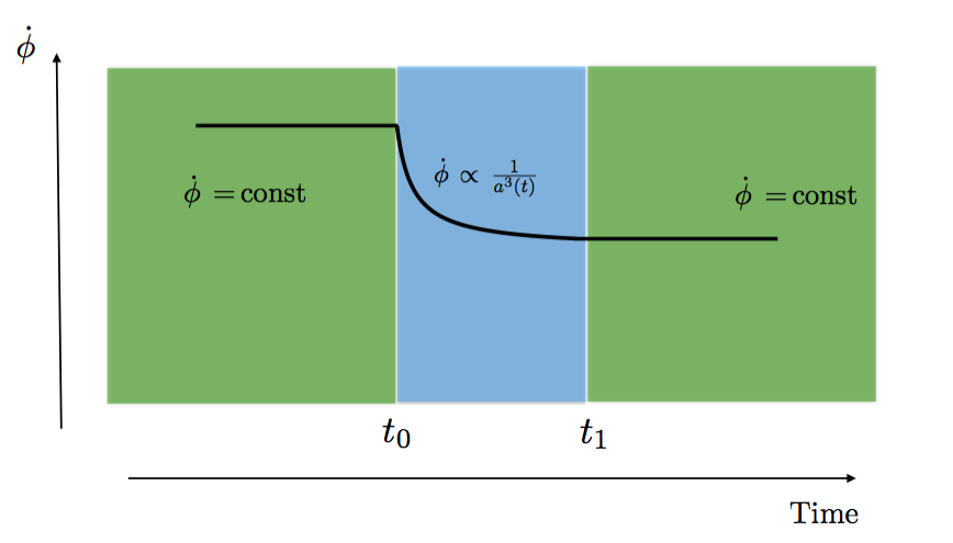
Figure 1: Schematic behaviour of the scalar field derivative in our system. Notice the intermediate non-attractor phase $\dot{\phi}\sim 1/a^{3}$. During the entire inflationary evolution the background geometry corresponds to pure de Sitter space.

From now on we make the hypothesis that $\alpha_{2}$ is very small such that for $t>t_{0}$ the system enters a short non-attractor phase, with rapidly decreasing field velocity

$$\dot{\phi}\propto\frac{1}{a^{3}}\,,$$ (40)

lasting from $t=t_{0}$ until $t\,=\,t_{1}$ when

$$\alpha_{2}\,\approx\frac{\alpha_{1}}{\,a^{3}(t_{1})}\,\frac{(-\rho_{2}+\delta_{2}+\beta_{2}+\sigma_{2})}{(-\rho_{1}+\delta_{1}+\beta_{1}+\sigma_{1})}\,.$$ (41)

For $t>t_{1}$ the scalar time derivative returns to being a constant, with value

$$\dot{\phi} = -\frac{H_{0}^{2}\,\alpha_{2}}{3\left(-\rho_{2}+\delta_{2}+\beta_{2}+\sigma_{2}\right)}\,.$$ (42)

The last phase of slow-roll evolution, $t>t_{1}$, is the least interesting one for our purposes – additional changes will be needed in the parameter space to gracefully exit the phase of pure de Sitter expansion, that will further modify the scalar profile. We do not consider this stage any further, since it occurs after the non-attractor regime we are interested in.

So far we have assumed that our background corresponds to a pure de Sitter universe, with constant Hubble parameter that we dub $H_{0}$ in all phases of evolution. Examining eq. (37), we learn that for $t<t_{0}$, when the scalar time derivative is constant, the Friedmann equation can be satisfied with constant Hubble parameter $H_{0}$, by choosing the constant potential $V_{1}$ as follows

$$V_{1}\,=\,\frac{H_{0}^{4}}{18}\,\frac{\alpha_{1}^{2}\left(-\rho_{1}+2\delta_{1}+3\beta_{1}+4\sigma_{1}\right)}{\left(-\rho_{1}+\beta_{1}+\delta_{1}+\sigma_{1}\right)^{2}}\,.$$ (43)

When $t>t_{0}$, the scalar field is rapidly varying, and at first sight it seems difficult to satisfy the Friedmann eq. (37) with $H(t)=H_{0}$ constant. But we can explore the non-linear structure of the kinetic sector of Horndeski action: we set the potential to zero, $V_{2}=0$, so that the background evolution eq. (37) becomes

$$0\,=\,\frac{\dot{\phi}^{2}}{2}\left(-\rho_{2}+2\,\delta_{2}\,\frac{H(t)}{H_{0}}+3\beta_{2}\frac{H^{2}(t)}{H_{0}^{2}}+4\sigma_{2}\frac{H^{3}(t)}{H_{0}^{3}}\right)\,.$$ (44)

The parenthesis in the previous equation is a polynomial in the Hubble parameter $H(t)$, and we can select our parameters so that it admits a real constant root: the choice we adopt for this purpose is

$$\rho_{2}\,=2\delta_{2}+3\beta_{2}+4\sigma_{2}\,,$$ (45)

which makes the parenthesis in eq. (44) vanish when $H(t)=H_{0}$. This is a ‘self-accelerating’ de Sitter branch of solutions, where the non-standard kinetic terms allow us to have a pure de Sitter expansion also in a phase where the scalar field is rapidly varying.

After determining the homogeneous background configurations for our system, we now analyze the behaviour of tensor and scalar fluctuations.

4.4 Dynamics of fluctuations

The dynamics of primordial tensor and scalar fluctuations for inflationary models based on Horndeski theory have been explored in detail [70]. See instead e.g. [87, 88] for systematic studies on the dynamics of cosmological fluctuations in inflationary models with parameter discontinuities. Tensor fluctuations around a FRW background metric with homogeneous scalar profile are controlled by the following quadratic action

$$S^{(2)}_{T} = \frac{1}{8}\int dt\,d^{3}x\,a^{3}\,\left[{\cal G}_{T}\left(\partial_{t}{h}_{ij}\right)^{2}-\frac{{\cal F}_{T}}{a^{2}}\,\left(\vec{\nabla}h_{ij}\right)^{2}\right]\,,$$ (46)

where (recall we are focussing on kinetically driven scenarios, where the functions $G_{a}$ only depend on $X$)

$${\cal G}_{T} = 2\,\left[G_{4}-2XG_{4X}-XH\dot{\phi}G_{5X}\right]\,,$$ (47)

$${\cal F}_{T} = 2\,\left[G_{4}-X\ddot{\phi}G_{5X}\right].$$ (48)

Scalar fluctuations are described by the quadratic action

$$S^{(2)}_{S} = \frac{1}{2}\int dt\,d^{3}x\,a^{3}\,\left[{\cal G}_{S}\left(\partial_{t}{\cal R}\right)^{2}-\frac{{\cal F}_{S}}{a^{2}}\,\left(\vec{\nabla}\cal R\right)^{2}\right]\,,$$ (49)

where:

$${\cal G}_{S} = \frac{\Sigma}{\Theta^{2}}\mathcal{G}_{T}^{2}+3\mathcal{G}_{T}\,,$$ (50)

$${\cal F}_{S} = \frac{1}{a}\frac{d}{dt}\left(\frac{a}{\Theta}\mathcal{G}_{T}^{2}\right)-\mathcal{F}_{T}\,,$$ (51)

and the explicit expressions of $\Sigma$ and $\Theta$ in terms of the functions $G_{a}$ are given in the appendix A. Tensor and scalar fluctuations are then characterised by the functions ${\cal G}_{T}$, ${\cal F}_{T}$, ${\cal G}_{S}$, ${\cal F}_{S}$ defined above. In the limit of very small $\alpha_{2}$ we are adopting

$$\alpha_{2}\ll 1\,,$$ (52)

which is the relevant regime to have a phase of non-attractor inflationary evolution, we find that each of these functions is proportional to $\dot{\phi}^{2}/H_{0}^{2}$ in both phases of evolution, namely:

$${\cal G}_{Ti} = g_{ti}\,\frac{\dot{\phi}^{2}}{H_{0}^{2}}\hskip 22.76228pt,\hskip 22.76228pt{\cal G}_{Si}\,=\,g_{si}\,\frac{\dot{\phi}^{2}}{H_{0}^{2}}\,,$$ (53)

$${\cal F}_{Ti} = f_{ti}\,\frac{\dot{\phi}^{2}}{H_{0}^{2}}\hskip 22.76228pt,\hskip 22.76228pt{\cal F}_{Si}\,=\,f_{si}\,\frac{\dot{\phi}^{2}}{H_{0}^{2}}\,.$$ (54)

The parameters $g_{ti}$, $g_{si}$, $f_{ti}$, $f_{si}$, are constant, and we need them to be positive to avoid instabilities.

In the first part of the evolution, $t\leq t_{0}$, we set $\delta_{1}=0$ (for simplicity) and find the following expressions for the constant parameters entering eqs. (53), (54),

$$f_{t1} = -\frac{\beta_{1}}{6}\,,$$ (55)

$$g_{t1} = \frac{\beta_{1}+3\sigma_{1}}{6}\,,$$ (56)

$$g_{s1} = \frac{\left(\beta_{1}+3\sigma_{1}\right)\left(3\beta_{1}^{2}+\rho_{1}(\beta_{1}+3\sigma_{1})+2\sigma_{1}(4\beta_{1}+3\sigma_{1})\right)}{18(\beta_{1}+2\sigma_{1})^{2}}\,,$$ (57)

while the quantity $f_{s1}$ satisfies the condition

$$f_{s1}\,=\,\frac{\left(f_{t1}-g_{t1}\right)^{2}}{2g_{t1}-f_{t1}}\,,$$ (58)

which relates its value to the remaining quantities. The stability of fluctuations in the first phase of the evolution thus requires the following relations: $\beta_{1}<0$, $\beta_{1}+3\sigma_{1}>0$ (implying $\sigma_{1}>0$) and $\beta_{1}+3\sigma_{1}>-\beta_{1}/2$. With these choices, one can easily satisfy $g_{s1}>0$ by choosing $\rho_{1}$ appropriately.

The second part of the evolution, $t_{0}\,<\,t\,<\,t_{1}$, is the most interesting since $\dot{\phi}\propto a^{-3}$ and we are in a non-attractor phase which enhances tensor fluctuations. In this case, we find that the parameters of eqs. (53), (54) read

$$f_{t2} = -\frac{\beta_{2}+9\sigma_{2}}{6}\,,$$ (59)

$$g_{t2} = \frac{\beta_{2}+3\sigma_{2}}{6}\,,$$ (60)

$$f_{s2} = \frac{-2\beta_{2}^{2}+\delta_{2}(\beta_{2}+9\sigma_{2})+3\sigma_{2}(\beta_{2}+3\sigma_{2})}{6\left(3\beta_{2}+\delta_{2}+6\sigma_{2}\right)}\,.$$ (61)

Moreover, we find the relations

$$g_{s2} = \frac{3}{5}\,\left(f_{s2}+f_{t2}+5g_{t2}\right)\,,$$ (62)

$$\rho_{2} = -\frac{f_{t2}\left(f_{s2}+f_{t2}\right)+19g_{t2}\left(f_{s2}+f_{t2}\right)+60g_{t2}^{2}}{f_{s2}+f_{t2}}\,,$$ (63)

where we used (45). Note that these relations imply $\rho_{2}<0$, and hence $g_{s2}>0$ whenever $f_{t2},g_{t2},f_{s2}>0$. Imposing the condition (45) in the second phase of the evolution, we require the following relations to hold in order to avoid instabilities of the tensor and scalar fluctuations: $\beta_{2}>0$, $\sigma_{2}<0$, $\delta_{2}<0$ where $\beta_{2}+9\sigma_{2}<0$, $\beta_{2}+3\sigma_{2}>0$ and $f_{s2}>0$ by choosing an appropriate $\delta_{2}$.

As we explained above, we are not interested in investigating the last stage of slow-roll evolution, for $t\geq t_{1}$ (see eq. (41)) when the size of the parameter $\alpha_{2}$ becomes important. This phase occurs after the non-attractor phase we wish to investigate, and the properties of the system and the evolution of fluctuations can change and are not necessarily described by the action we are interested in.

We now analyse an explicit choice of quantities within the available parameter space which satisfies the aforementioned stability conditions, and discuss the corresponding physical consequences. See also appendix B for an investigation of our system in a ‘Einstein frame’ where tensor fluctuation at quadratic order obey a standard action.

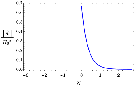
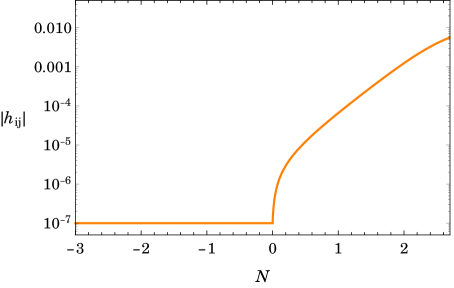
Figure 2: The behavior of $\dot{\phi}$ and $|h_{ij}|$ through the transition to the non-attractor phase where we used the expressions (4.3) and (8) respectively. On the right, we have set $\mathcal{C}_{2}=\mathcal{C}_{1}(H_{0}/c_{T})$ with $\mathcal{C}_{1}=10^{-7}$ in (8) to show the evolution of $|h_{ij}|$. For both plots, we have the following choice of parameters: $\alpha_{1}=1,\,\beta_{1}=-1,\,\sigma_{1}=2.5,\,\rho_{1}=1,\,\delta_{1}\,=\,0$, $\alpha_{2}\,=\,10^{-3},\,\beta_{2}\,=\,1.5,\,\sigma_{2}\,=\,-0.2,\,\delta_{2}\,=\,-4,\,\rho_{2}\,=\,-4.3$ where $N=0$ corresponds to the transition point. In these plots, the non-attractor phase lasts approximately $\Delta N\simeq 2.7$ e-folds.

Enhancement of spectra of fluctuations during the non-attractor phase

In the non-attractor phase we are considering, both tensor and scalar fluctuations can be enhanced. The tensor pump field during the non-attractor phase is given by

$$\tilde{z}_{T}=\frac{a}{2}\left({\cal G}_{T}{\cal F}_{T}\right)^{1/4}\,=\,\frac{a\dot{\phi}}{2H_{0}}\,(g_{t2}f_{t2})^{1/4}\,,$$ (64)

whereas the scalar pump field is given by the following expression:

$$\tilde{z}_{S}=\sqrt{2}a\left({\cal G}_{S}{\cal F}_{S}\right)^{1/4}=\,\frac{\sqrt{2}a\dot{\phi}}{H_{0}}\,(g_{s2}f_{s2})^{1/4}\,.$$ (65)

In both of the expressions for $\tilde{z}_{T}$ and $\tilde{z}_{S}$, the scalar field velocity reads

$$\dot{\phi}\approx-\frac{H_{0}^{2}\,\alpha_{1}}{3\left(-\rho_{1}+\delta_{1}+\beta_{1}+\sigma_{1}\right)}\,a^{-3}\,.$$ (66)

As $\dot{\phi}\propto a^{-3}$, we realise the condition (23) we identified before. We therefore realize the tensor duality and as can be anticipated from the expression in (22), we will have an enhancement of the tensor power spectrum: modes that leave the horizon within the time interval $t_{0}\,<\,t\,<\,t_{1}$ corresponding to the non-attractor phase will receive an exponential enhancement proportional to $a^{6}$. Notice that since fluctuations evolve beyond the Hubble horizon, the tensor and scalar power spectra should be evaluated at the end of the non-attractor phase which we denote by $t_{1}$. Therefore, using (41), the tensor power spectrum at the end of the non-attractor phase can be amplified with respect to the one during the preceeding slow-roll by the following amount

$$\frac{{\cal P}_{\tilde{h}}}{{\cal P}_{h}}~{}~{}\bigg{\rvert}_{t=t_{1}}\,=\,\left(\frac{z_{T}}{\tilde{z}_{T}}\right)^{2}\,\bigg{\rvert}_{t=t_{1}} = a(t_{1})^{6}\left(\frac{g_{t1}f_{t1}}{g_{t2}f_{t2}}\right)^{1/2}$$ (67)

$$\simeq \left(\frac{\alpha_{1}}{\alpha_{2}}\right)^{2}\,\frac{(-\rho_{2}+\delta_{2}+\beta_{2}+\sigma_{2})^{2}}{(-\rho_{1}+\delta_{1}+\beta_{1}+\sigma_{1})^{2}}\left(\frac{\beta_{1}(\beta_{1}+3\sigma_{1})}{(\beta_{2}+3\sigma_{2})(\beta_{2}+9\sigma_{2})}\right)^{1/2}.$$

It is worth emphasizing again that we can enhance the power in the fluctuations while maintaining a scale invariant statistics deep in the non-attractor regime. This behavior can be particularly interesting to build models with an enhanced tensor power spectrum detectable at interferometer scales, see the brief discussion in section 5. See also [89] for a scenario able to amplify the tensor-to-scalar ratio $r$ at small scales, by reducing the size of the spectrum of scalar fluctuations.

Similarly to the tensor fluctuations, scalar fluctuations grow during the non-attractor regime since the scalar pump field $\tilde{z}_{S}$ has a similar structure to $\tilde{z}_{T}$. Using Wands’ duality (see footnote 1) we have

$$\frac{{\cal P}_{\tilde{\mathcal{R}}}}{{\cal P}_{\mathcal{R}}}~{}~{}\bigg{\rvert}_{t=t_{1}}\,=\,\left(\frac{z_{S}}{\tilde{z}_{S}}\right)^{2}\,\bigg{\rvert}_{t=t_{1}}=a^{6}(t_{1})\,\left(\frac{g_{s1}f_{s1}}{g_{s2}f_{s2}}\right)^{1/2},$$ (68)

where $g_{s1}$, $f_{s1}$, $f_{s2}$ and $g_{s2}$ defined as in (57),(58), (61) and (62) respectively.

As a specific example, we take the following set of parameters

$$\left({\alpha_{i},\beta_{i},\,\delta_{i},\,\rho_{i},\,\sigma_{i}}\right)\,=\,\left\{\begin{array}[]{l}\left({1,\,-1,\,0,\,1,\,2.5}\right)\hskip 139.41832ptt\,<\,t_{0}\\ \\ \left({10^{-3},\,1.5,\,-4,\,-4.3,\,-0.2}\right)\hskip 85.35826ptt\,>\,t_{0}.\end{array}\right.$$ (69)

For this choice, the corresponding field velocity $\dot{\phi}$ and the amplification of $|h_{ij}|$ using the super-horizon expression in (8) are shown in Figure 2. However, we reiterate that equation (8) can be only used as a rough indicator of the enhancement of the fluctuations as it relies on strict super-horizon limit $k=0$ (see [69] ). On the other hand, to obtain a more accurate estimate on the enhancement we use the expressions based on the duality in (67) and (68) with the parameter choices in (69). We find that the tensor power spectrum can be enhanced by a factor of $\approx 5\times 10^{7}$ and the scalar power spectrum by a factor of $\approx 5\times 10^{6}$ while the system satisfies all the stability constraints in both sectors. In general, looking at the structure of the equations (68) and (67), we see that the level of enhancement of the scalar and tensor power spectrum is mainly controlled by the duration of the non-attractor regime, in particular by the ratio $\alpha_{1}/\alpha_{2}$ whereas the other parameters in the model mainly serve to satisfy the stability conditions of the fluctuations.

We finally comment on the propagation speed of the fluctuations in the model we consider in this paper. As both the scalar and tensor fluctuations have kinetic functions that satisfy the relations: ${\cal F}_{T}\neq{\cal G}_{T}$ and ${\cal F}_{S}\neq{\cal G}_{S}$, they exhibit non-trivial sound speeds given by the following expressions

$$c_{S}^{2}\,=\,\left\{\begin{array}[]{l}f_{s1}/g_{s1}\,,\hskip 56.9055ptt\,<\,t_{0}\,,\\ \\ f_{s2}/g_{s2}\,,\hskip 56.9055ptt\,>\,t_{0}\,,\end{array}\right.$$ (70)

and

$$c_{T}^{2}\,=\,\left\{\begin{array}[]{l}f_{t1}/g_{t1}\,,\hskip 56.9055ptt\,<\,t_{0}\,,\\ \\ f_{t2}/g_{t2}\,,\hskip 56.9055ptt\,>\,t_{0}\,.\end{array}\right.$$ (71)

For the specific parameter choices we made in (69), we learn that during both phases of the inflationary evolution, for $t<t_{0}$ and $t>t_{0}$, the scalar and tensor sound speed is less than unity, i.e $c_{T}^{2}<1$ and $c_{S}^{2}<1$. In particular, in the slow-roll phase, the tensor sound speed is $c_{T}^{2}\approx 0.15$ and it increases to $c_{T}^{2}=0.33$ during the non-attractor phase. Similarly, scalar sound speed is given by $c_{S}^{2}\approx 0.69$ during the slow-roll era and increases to $c_{S}^{2}\approx 0.89$ in the non-attractor era.

Non-gaussianity

We conclude this section with some comments on tensor non-Gaussianity, an observable that can be useful for discriminating among primordial and astrophysical stochastic gravitational wave background detectable with interferometers [90]. Tensor non-Gaussianity is also an important observable for charactizing the primordial stochastic gravitational wave background at CMB scales, and have been explored in other contexts, see e.g. [91, 47, 50]. We briefly consider tensor non-Gaussianity with a shape enhanced in the squeezed limit: other shapes of tensor non-Gaussianity can be produced in single field inflation – see [92] – but we do not consider them in this context. This shape is controlled by the following third order action, obtained by expanding up to third order in tensor fluctuations the Horndeski set-up we are examining [92]

$$S_{T}^{(3)}\,=\,\int dt\,d^{3}x\,a\,\frac{{\cal F}_{T}}{4}\,\left(h_{ik}h_{jl}-\frac{1}{2}h_{ij}h_{kl}\right)\,\partial_{k}\partial_{l}\,h_{ij}\,.$$ (72)

Considering the tensor dual of a slow-roll phase as described in section 3, we learn that in terms of the tensor dual variable $\tilde{h}_{ij}\,=\,\left(z_{T}/\tilde{z}_{T}\right)\,h_{ij}$ the overall factor in the previous third order action changes to

$$S_{\tilde{T}}^{(3)}\,=\,\int dt\,d^{3}x\,a\,\frac{{\cal F}_{T}}{4}\,\left(\frac{z_{T}}{\tilde{z}_{T}}\right)^{3}\,\left(\tilde{h}_{ik}\tilde{h}_{jl}-\frac{1}{2}\tilde{h}_{ij}\tilde{h}_{kl}\right)\,\partial_{k}\partial_{l}\,\tilde{h}_{ij}\,.$$ (73)

Hence, if the ratio $z_{T}/\tilde{z}_{T}$ is large as for the tensor dual of a slow-roll phase, see Section 3.1, the amplitude of squeezed tensor non-Gaussianity can increase in the tensor dual regime. It would be interesting to develop further this subject, and investigate its consequences for the detectability of tensor non-Gaussianity at interferometers, as explored in [90]. We plan to do so in a forthcoming work.

5 Outlook

In this work we discussed a new mechanism to amplify tensor fluctuations during single field inflation, by exploiting a phase of non-attractor evolution. We have identified the necessary condition for amplifying the tensor spectrum at super-horizon scales, which is that the tensor pump field, defined in eq. (6), decreases with time during a phase of the inflationary evolution. The would-be decaying tensor mode gets then enhanced and increases the size of tensor fluctuations. We determined a criterium, which we dub tensor duality, that allows us to analytically estimate the statistical properties of the amplified tensor fluctuations during the non-attractor era. We then built and investigated in detail a concrete model of kinetically driven inflation able to satisfy our conditions, and analytically determined the properties of the enhanced spectrum of tensor modes in this set-up. Much work is left for the future:

• Our concrete scenario is based on G-inflation, since we need a non-trivial kinetic mixing between scalar and metric to realise our mechanism. It will be interesting to understand whether other realisations can exist, for example by means of sudden changes in the tensor sound speed due to effects of new heavy physics or string theory, as in [93].

• The quadratic tensor action we obtained in our system is distinct from the one of single field inflation with standard kinetic terms, but a sequence of conformal and disformal transformations can recast it in standard form [94]. In Appendix B we show that our system, during the non-attractor era we have investigated, can be disformally related to a rapidly contracting universe. It will be interesting to further explore the physical implications of disformal transformations during non-attractor regimes.

• We provided evidence that the spectrum of tensor fluctuations can be non-Gaussian, besides being enhanced. It will be important to analytically study in more details the amplitude and shape of non-Gaussianity of tensor modes in our set-up.

• Finally, it will be important to build a complete, realistic scenario (based on G-inflation or on other theories) able to sufficiently amplify tensor modes at interferometer scales, and study prospects for the detectability of the stochastic primordial tensor background and its non-Gaussianity.

We hope to further report soon on these topics.

Acknowledgments

MM, OÖ, GT and IZ are partially supported by the STFC grant ST/P00055X/1.

Appendix A Background equations in Generalized G-Inflation and functions $\Sigma$ and $\Theta$

In a FRW universe, the equations describing the background evolution can be written in an analogous way to the minimally coupled canonical scalar field. Since we are dealing with a shift symmetric system, the background equations are simpler compared to the general expressions given in [70]. In this case, the generalized energy and the sum of energy and pressure densities can be expressed in the following way

$$\dot{\phi}J-G_{2}+2X\left[6H^{2}G_{4X}+2H^{3}\dot{\phi}G_{5X}\right]=6H^{2}G_{4},$$ (74)

$$\dot{\phi}J-2X\ddot{\phi}G_{3X}+2\frac{{\rm d}}{{\rm d}t}\left[2H(G_{4}-2XG_{4X})-H^{2}X\dot{\phi}G_{5X}\right]=0,$$ (75)

where

$$J=\dot{\phi}\left[G_{2X}+3H\dot{\phi}G_{3X}+6H^{2}(G_{4X}+2XG_{4XX})+H^{3}\dot{\phi}(3G_{5X}+2XG_{5XX})\right]$$ (76)

The generalized Friedman equations above can be combined with the scalar-field equation

$$\frac{1}{a^{3}}\frac{{\rm d}}{{\rm d}t}(a^{3}J)=0\,,$$ (77)

to close the system of equations. On the other hand, the functions $\Sigma$ and $\Theta$ appearing in the kinetic functions $\mathcal{F}_{S}$ and $\mathcal{G}_{S}$ (50) of the scalar fluctuations are given by the following expressions

$$\Sigma\equiv XG_{2X}+2X^{2}G_{2XX} +12H\dot{\phi}XG_{3X}+6H\dot{\phi}X^{2}G_{3XX}-6H^{2}G_{4}$$

$$+6H^{2}(7XG_{4X}+16X^{2}G_{4XX}+4X^{3}G_{4XXX})$$

$$+30H^{3}\dot{\phi}XG_{5X}+26H^{3}\dot{\phi}X^{2}G_{5XX}+4H^{3}\dot{\phi}X^{3}G_{5XXX},$$ (78)

and

$$\Theta=-\dot{\phi}XG_{3X}+2HG_{4}-8HXG_{4X}-8HX^{2}G_{4XX}-H^{2}\dot{\phi}(5XG_{5X}+2X^{2}G_{5XX}).$$ (79)

Appendix B Disformal and conformal transformation of the tensor action

In [94] it has been shown that a combination of conformal and disformal transformations allows one to recast the quadratic tensorial action into a form identical to the action of tensor modes in standard slow-roll inflation. See also [95] for an analysis of the consequences of disformal transformation for cosmological fluctuations. We discuss the implications of such transformations for our set-up.

We follow the prescription of [94, 96] in defining the conformal and disformal transformations, and we redefine the time coordinate and scale factor as

$$\begin{split}{\rm d}{t}=(c_{T}\mathcal{F}_{T})^{-1/2}~{}{\rm d}{\hat{t}},\quad a=\left(\frac{c_{T}}{\mathcal{F}_{T}}\right)^{1/2}\hat{a}.\end{split}$$ (80)

(here $c_{T}^{2}\,=\,\mathcal{F}_{T}/\mathcal{G}_{T}$) to ensure the metric acquires a standard FRW form. With these redefinitions, the tensor action now reads

$$\begin{split}S&=\frac{1}{8}\int d{\hat{t}}\,d^{3}{x}\,\hat{a}^{3}\bigg{[}(\partial_{\hat{t}}h_{ij})^{2}-(\nabla h_{ij})^{2}\bigg{]}.\end{split}$$ (81)

as in standard single field inflation in an Einstein frame. Using relations (80), we can compare the Hubble parameter associated with the new scale factor $\hat{a}(\hat{t})$ with the quantities defined in terms of the original time $t$:

$$\hat{H}=\frac{1}{\hat{a}}\frac{d\,\hat{a}}{d\hat{t}}=(c_{T}\mathcal{F}_{T})^{-1/2}\left[H+\frac{1}{2}\left(\frac{\dot{\mathcal{F}_{T}}}{\mathcal{F}_{T}}-\frac{\dot{c}_{T}}{c_{T}}\right)\right],$$ (82)

We then use the structure of the relations (53), (54) to evaluate the right hand side of (82). When focussing on the first phase of slow-roll regime, we find, as expected, that the new Hubble parameter $\hat{H}$ is proportional to the original one $H$.

But when evaluated in the non-attractor phase, using the relations (see eqs (53) and (54))

$${\cal F}_{T}=f_{t2}\,\frac{\dot{\phi}^{2}}{H_{0}^{2}},~{}~{}~{}~{}~{}~{}{\cal G}_{T}=g_{t2}\,\frac{\dot{\phi}^{2}}{H_{0}^{2}},~{}~{}~{}~{}~{}~{}c_{T}=\sqrt{\frac{f_{t2}}{g_{t2}}}$$ (83)

and the fact that $\dot{\phi}\,=\,\phi_{0}/a^{3}$ for a constant $\phi_{0}$, we find the following expresion for the Hubble parameter in the Einstein frame

$$\hat{H}\, = \,-\frac{2\,g_{t2}^{1/4}H^{2}\,a^{3}}{\,f_{t2}^{3/4}\,|\phi_{0}|}\,,$$ (84)

$$= -\sqrt{\frac{4H\phi_{0}g_{t2}^{5/4}}{f_{t2}^{3/4}}}~{}~{}\hat{a}^{-3/2},$$ (85)

where in the second line we used the second relation in (80) between the scale factors in the two frames. Hence in the Einstein frame where tensor fluctuations are controlled by action (81), the background geometry in the non-attractor regime is described in terms of a dust dominated contracting universe.

This impliest that, within the Einstein frame description developed in this appendix, the Universe undergoes a short phase of contraction - lasting a few e-folds - during which the amplitude of tensor fluctuations can grow. This perspective offers another point of view for the results in the main text, within a frame where the action for quadratic tensor fluctuations is standard. It would be interesting to embed our scenario in a set-up with smooth transition between expanding and contracting phases, and study in detail the matching and stability issues for fluctuations. Possible instabilities in the bouncing transition phase can be tamed in sufficiently rich scalar-tensor systems related to the set-up we use in this work. A detailed analysis of this subject is beyond the scope of this article, and we leave it for future investigations.

References

- [1] V. F. Mukhanov, H. A. Feldman, and R. H. Brandenberger, “Theory of cosmological perturbations. Part 1. Classical perturbations. Part 2. Quantum theory of perturbations. Part 3. Extensions,” Phys. Rept. 215 (1992) 203–333.
- [2] S. Inoue and J. Yokoyama, “Curvature perturbation at the local extremum of the inflaton’s potential,” Phys. Lett. B524 (2002) 15–20, arXiv:hep-ph/0104083 [hep-ph].
- [3] A. D. Linde, “Fast roll inflation,” JHEP 11 (2001) 052, arXiv:hep-th/0110195 [hep-th].
- [4] W. H. Kinney, “Horizon crossing and inflation with large eta,” Phys. Rev. D72 (2005) 023515, arXiv:gr-qc/0503017 [gr-qc].
- [5] J. Martin, H. Motohashi, and T. Suyama, “Ultra Slow-Roll Inflation and the non-Gaussianity Consistency Relation,” Phys. Rev. D87 no. 2, (2013) 023514, arXiv:1211.0083 [astro-ph.CO].
- [6] H. Motohashi, A. A. Starobinsky, and J. Yokoyama, “Inflation with a constant rate of roll,” JCAP 1509 (2015) 018, arXiv:1411.5021 [astro-ph.CO].
- [7] Z. Yi and Y. Gong, “On the constant-roll inflation,” JCAP 1803 no. 03, (2018) 052, arXiv:1712.07478 [gr-qc].
- [8] K. Dimopoulos, “Ultra slow-roll inflation demystified,” Phys. Lett. B775 (2017) 262–265, arXiv:1707.05644 [hep-ph].
- [9] C. Pattison, V. Vennin, H. Assadullahi, and D. Wands, “The attractive behaviour of ultra-slow-roll inflation,” arXiv:1806.09553 [astro-ph.CO].
- [10] A. A. Starobinsky, “Spectrum of adiabatic perturbations in the universe when there are singularities in the inflation potential,” JETP Lett. 55 (1992) 489–494. [Pisma Zh. Eksp. Teor. Fiz.55,477(1992)].
- [11] D. Wands, “Duality invariance of cosmological perturbation spectra,” Phys. Rev. D60 (1999) 023507, arXiv:gr-qc/9809062 [gr-qc].
- [12] J. Garcia-Bellido, “Massive Primordial Black Holes as Dark Matter and their detection with Gravitational Waves,” J. Phys. Conf. Ser. 840 no. 1, (2017) 012032, arXiv:1702.08275 [astro-ph.CO].
- [13] M. Sasaki, T. Suyama, T. Tanaka, and S. Yokoyama, “Primordial black holes?perspectives in gravitational wave astronomy,” Class. Quant. Grav. 35 no. 6, (2018) 063001, arXiv:1801.05235 [astro-ph.CO].
- [14] B. Carr, F. Kuhnel, and M. Sandstad, “Primordial Black Holes as Dark Matter,” Phys. Rev. D94 no. 8, (2016) 083504, arXiv:1607.06077 [astro-ph.CO].
- [15] J. Garcia-Bellido and E. Ruiz Morales, “Primordial black holes from single field models of inflation,” Phys. Dark Univ. 18 (2017) 47–54, arXiv:1702.03901 [astro-ph.CO].
- [16] C. Germani and T. Prokopec, “On primordial black holes from an inflection point,” Phys. Dark Univ. 18 (2017) 6–10, arXiv:1706.04226 [astro-ph.CO].
- [17] H. Motohashi and W. Hu, “Primordial Black Holes and Slow-Roll Violation,” Phys. Rev. D96 no. 6, (2017) 063503, arXiv:1706.06784 [astro-ph.CO].
- [18] G. Ballesteros and M. Taoso, “Primordial black hole dark matter from single field inflation,” Phys. Rev. D97 no. 2, (2018) 023501, arXiv:1709.05565 [hep-ph].
- [19] J. M. Ezquiaga, J. Garcia-Bellido, and E. Ruiz Morales, “Primordial Black Hole production in Critical Higgs Inflation,” Phys. Lett. B776 (2018) 345–349, arXiv:1705.04861 [astro-ph.CO].
- [20] M. Cicoli, V. A. Diaz, and F. G. Pedro, “Primordial Black Holes from String Inflation,” JCAP 1806 no. 06, (2018) 034, arXiv:1803.02837 [hep-th].
- [21] O. Ozsoy, S. Parameswaran, G. Tasinato, and I. Zavala, “Mechanisms for Primordial Black Hole Production in String Theory,” JCAP 1807 no. 07, (2018) 005, arXiv:1803.07626 [hep-th].
- [22] M. Biagetti, G. Franciolini, A. Kehagias, and A. Riotto, “Primordial Black Holes from Inflation and Quantum Diffusion,” JCAP 1807 no. 07, (2018) 032, arXiv:1804.07124 [astro-ph.CO].
- [23] R. Saito, J. Yokoyama, and R. Nagata, “Single-field inflation, anomalous enhancement of superhorizon fluctuations, and non-Gaussianity in primordial black hole formation,” JCAP 0806 (2008) 024, arXiv:0804.3470 [astro-ph].
- [24] K. Kannike, L. Marzola, M. Raidal, and H. Veerm e, “Single Field Double Inflation and Primordial Black Holes,” JCAP 1709 no. 09, (2017) 020, arXiv:1705.06225 [astro-ph.CO].
- [25] S. Chongchitnan and G. Efstathiou, “Prospects for direct detection of primordial gravitational waves,” Phys. Rev. D73 (2006) 083511, arXiv:astro-ph/0602594 [astro-ph].
- [26] M. Kamionkowski and E. D. Kovetz, “The Quest for B Modes from Inflationary Gravitational Waves,” Ann. Rev. Astron. Astrophys. 54 (2016) 227–269, arXiv:1510.06042 [astro-ph.CO].
- [27] M. Maggiore, Gravitational Waves. Vol. 1: Theory and Experiments. Oxford Master Series in Physics. Oxford University Press, 2007. http://www.oup.com/uk/catalogue/?ci=9780198570745.
- [28] M. Maggiore, Gravitational Waves. Vol. 2: Astrophysics and Cosmology. Oxford University Press, 2018.
- [29] J. L. Cook and L. Sorbo, “Particle production during inflation and gravitational waves detectable by ground-based interferometers,” Phys. Rev. D85 (2012) 023534, arXiv:1109.0022 [astro-ph.CO]. [Erratum: Phys. Rev.D86,069901(2012)].
- [30] L. Senatore, E. Silverstein, and M. Zaldarriaga, “New Sources of Gravitational Waves during Inflation,” JCAP 1408 (2014) 016, arXiv:1109.0542 [hep-th].
- [31] D. Carney, W. Fischler, E. D. Kovetz, D. Lorshbough, and S. Paban, “Rapid field excursions and the inflationary tensor spectrum,” JHEP 11 (2012) 042, arXiv:1209.3848 [hep-th].
- [32] M. Biagetti, M. Fasiello, and A. Riotto, “Enhancing Inflationary Tensor Modes through Spectator Fields,” Phys. Rev. D88 (2013) 103518, arXiv:1305.7241 [astro-ph.CO].
- [33] M. Biagetti, E. Dimastrogiovanni, M. Fasiello, and M. Peloso, “Gravitational Waves and Scalar Perturbations from Spectator Fields,” JCAP 1504 (2015) 011, arXiv:1411.3029 [astro-ph.CO].
- [34] C. Goolsby-Cole and L. Sorbo, “Nonperturbative production of massless scalars during inflation and generation of gravitational waves,” JCAP 1708 no. 08, (2017) 005, arXiv:1705.03755 [astro-ph.CO].
- [35] L. Sorbo, “Parity violation in the Cosmic Microwave Background from a pseudoscalar inflaton,” JCAP 1106 (2011) 003, arXiv:1101.1525 [astro-ph.CO].
- [36] M. M. Anber and L. Sorbo, “Non-Gaussianities and chiral gravitational waves in natural steep inflation,” Phys. Rev. D85 (2012) 123537, arXiv:1203.5849 [astro-ph.CO].
- [37] N. Barnaby and M. Peloso, “Large Nongaussianity in Axion Inflation,” Phys. Rev. Lett. 106 (2011) 181301, arXiv:1011.1500 [hep-ph].
- [38] N. Barnaby, J. Moxon, R. Namba, M. Peloso, G. Shiu, and P. Zhou, “Gravity waves and non-Gaussian features from particle production in a sector gravitationally coupled to the inflaton,” Phys. Rev. D86 (2012) 103508, arXiv:1206.6117 [astro-ph.CO].
- [39] O. Ozsoy, “On Synthetic Gravitational Waves from Multi-field Inflation,” JCAP 1804 no. 04, (2018) 062, arXiv:1712.01991 [astro-ph.CO].
- [40] A. Maleknejad and M. M. Sheikh-Jabbari, “Gauge-flation: Inflation From Non-Abelian Gauge Fields,” Phys. Lett. B723 (2013) 224–228, arXiv:1102.1513 [hep-ph].
- [41] E. Dimastrogiovanni and M. Peloso, “Stability analysis of chromo-natural inflation and possible evasion of Lyth’s bound,” Phys. Rev. D87 no. 10, (2013) 103501, arXiv:1212.5184 [astro-ph.CO].
- [42] P. Adshead, E. Martinec, and M. Wyman, “Gauge fields and inflation: Chiral gravitational waves, fluctuations, and the Lyth bound,” Phys. Rev. D88 no. 2, (2013) 021302, arXiv:1301.2598 [hep-th].
- [43] P. Adshead, E. Martinec, and M. Wyman, “Perturbations in Chromo-Natural Inflation,” JHEP 09 (2013) 087, arXiv:1305.2930 [hep-th].
- [44] I. Obata, T. Miura, and J. Soda, “Chromo-Natural Inflation in the Axiverse,” Phys. Rev. D92 no. 6, (2015) 063516, arXiv:1412.7620 [hep-ph]. [Addendum: Phys. Rev.D95,no.10,109902(2017)].
- [45] A. Maleknejad, “Axion Inflation with an SU(2) Gauge Field: Detectable Chiral Gravity Waves,” JHEP 07 (2016) 104, arXiv:1604.03327 [hep-ph].
- [46] E. Dimastrogiovanni, M. Fasiello, and T. Fujita, “Primordial Gravitational Waves from Axion-Gauge Fields Dynamics,” JCAP 1701 no. 01, (2017) 019, arXiv:1608.04216 [astro-ph.CO].
- [47] A. Agrawal, T. Fujita, and E. Komatsu, “Large Tensor Non-Gaussianity from Axion-Gauge Fields Dynamics,” arXiv:1707.03023 [astro-ph.CO].
- [48] P. Adshead and E. I. Sfakianakis, “Higgsed Gauge-flation,” JHEP 08 (2017) 130, arXiv:1705.03024 [hep-th].
- [49] R. R. Caldwell and C. Devulder, “Axion Gauge Field Inflation and Gravitational Leptogenesis: A Lower Bound on B Modes from the Matter-Antimatter Asymmetry of the Universe,” Phys. Rev. D97 no. 2, (2018) 023532, arXiv:1706.03765 [astro-ph.CO].
- [50] A. Agrawal, T. Fujita, and E. Komatsu, “Tensor Non-Gaussianity from Axion-Gauge-Fields Dynamics : Parameter Search,” arXiv:1802.09284 [astro-ph.CO].
- [51] J. R. Espinosa, D. Racco, and A. Riotto, “A Cosmological Signature of the SM Higgs Instability: Gravitational Waves,” arXiv:1804.07732 [hep-ph].
- [52] S. Endlich, A. Nicolis, and J. Wang, “Solid Inflation,” JCAP 1310 (2013) 011, arXiv:1210.0569 [hep-th].
- [53] N. Bartolo, D. Cannone, A. Ricciardone, and G. Tasinato, “Distinctive signatures of space-time diffeomorphism breaking in EFT of inflation,” JCAP 1603 no. 03, (2016) 044, arXiv:1511.07414 [astro-ph.CO].
- [54] A. Ricciardone and G. Tasinato, “Primordial gravitational waves in supersolid inflation,” Phys. Rev. D96 no. 2, (2017) 023508, arXiv:1611.04516 [astro-ph.CO].
- [55] A. Ricciardone and G. Tasinato, “Anisotropic tensor power spectrum at interferometer scales induced by tensor squeezed non-Gaussianity,” JCAP 1802 no. 02, (2018) 011, arXiv:1711.02635 [astro-ph.CO].
- [56] G. Domènech, T. Hiramatsu, C. Lin, M. Sasaki, M. Shiraishi, and Y. Wang, “CMB Scale Dependent Non-Gaussianity from Massive Gravity during Inflation,” JCAP 1705 no. 05, (2017) 034, arXiv:1701.05554 [astro-ph.CO].
- [57] G. Ballesteros, D. Comelli, and L. Pilo, “Massive and modified gravity as self-gravitating media,” Phys. Rev. D94 no. 12, (2016) 124023, arXiv:1603.02956 [hep-th].
- [58] D. Cannone, J.-O. Gong, and G. Tasinato, “Breaking discrete symmetries in the effective field theory of inflation,” JCAP 1508 no. 08, (2015) 003, arXiv:1505.05773 [hep-th].
- [59] C. Lin and L. Z. Labun, “Effective Field Theory of Broken Spatial Diffeomorphisms,” JHEP 03 (2016) 128, arXiv:1501.07160 [hep-th].
- [60] D. Cannone, G. Tasinato, and D. Wands, “Generalised tensor fluctuations and inflation,” JCAP 1501 no. 01, (2015) 029, arXiv:1409.6568 [astro-ph.CO].
- [61] M. Akhshik, “Clustering Fossils in Solid Inflation,” JCAP 1505 no. 05, (2015) 043, arXiv:1409.3004 [astro-ph.CO].
- [62] C. Lin and M. Sasaki, “Resonant Primordial Gravitational Waves Amplification,” Phys. Lett. B752 (2016) 84–88, arXiv:1504.01373 [astro-ph.CO].
- [63] M. Biagetti, E. Dimastrogiovanni, and M. Fasiello, “Possible signatures of the inflationary particle content: spin-2 fields,” JCAP 1710 no. 10, (2017) 038, arXiv:1708.01587 [astro-ph.CO].
- [64] E. Dimastrogiovanni, M. Fasiello, and G. Tasinato, “Probing the inflationary particle content: extra spin-2 field,” JCAP 1808 no. 08, (2018) 016, arXiv:1806.00850 [astro-ph.CO].
- [65] T. Fujita, S. Kuroyanagi, S. Mizuno, and S. Mukohyama, “Blue-tilted Primordial Gravitational Waves from Massive Gravity,” arXiv:1808.02381 [gr-qc].
- [66] N. Bartolo et al., “Science with the space-based interferometer LISA. IV: Probing inflation with gravitational waves,” JCAP 1612 no. 12, (2016) 026, arXiv:1610.06481 [astro-ph.CO].
- [67] O. Seto, J. Yokoyama, and H. Kodama, “What happens when the inflaton stops during inflation,” Phys. Rev. D61 (2000) 103504, arXiv:astro-ph/9911119 [astro-ph].
- [68] S. M. Leach and A. R. Liddle, “Inflationary perturbations near horizon crossing,” Phys. Rev. D63 (2001) 043508, arXiv:astro-ph/0010082 [astro-ph].
- [69] S. M. Leach, M. Sasaki, D. Wands, and A. R. Liddle, “Enhancement of superhorizon scale inflationary curvature perturbations,” Phys. Rev. D64 (2001) 023512, arXiv:astro-ph/0101406 [astro-ph].
- [70] T. Kobayashi, M. Yamaguchi, and J. Yokoyama, “Generalized G-inflation: Inflation with the most general second-order field equations,” Prog. Theor. Phys. 126 (2011) 511–529, arXiv:1105.5723 [hep-th].
- [71] F. Finelli and R. Brandenberger, “On the generation of a scale invariant spectrum of adiabatic fluctuations in cosmological models with a contracting phase,” Phys. Rev. D65 (2002) 103522, arXiv:hep-th/0112249 [hep-th].
- [72] M. Gasperini and G. Veneziano, “The Pre - big bang scenario in string cosmology,” Phys. Rept. 373 (2003) 1–212, arXiv:hep-th/0207130 [hep-th].
- [73] S. Gratton, J. Khoury, P. J. Steinhardt, and N. Turok, “Conditions for generating scale-invariant density perturbations,” Phys. Rev. D69 (2004) 103505, arXiv:astro-ph/0301395 [astro-ph].
- [74] L. A. Boyle, P. J. Steinhardt, and N. Turok, “A New duality relating density perturbations in expanding and contracting Friedmann cosmologies,” Phys. Rev. D70 (2004) 023504, arXiv:hep-th/0403026 [hep-th].
- [75] Y.-S. Piao, “On the dualities of primordial perturbation spectrums,” Phys. Lett. B606 (2005) 245–250, arXiv:hep-th/0404002 [hep-th].
- [76] L. E. Allen and D. Wands, “Cosmological perturbations through a simple bounce,” Phys. Rev. D70 (2004) 063515, arXiv:astro-ph/0404441 [astro-ph].
- [77] J. Khoury and F. Piazza, “Rapidly-Varying Speed of Sound, Scale Invariance and Non-Gaussian Signatures,” JCAP 0907 (2009) 026, arXiv:0811.3633 [hep-th].
- [78] J. Khoury and G. E. J. Miller, “Towards a Cosmological Dual to Inflation,” Phys. Rev. D84 (2011) 023511, arXiv:1012.0846 [hep-th].
- [79] D. Battefeld and P. Peter, “A Critical Review of Classical Bouncing Cosmologies,” Phys. Rept. 571 (2015) 1–66, arXiv:1406.2790 [astro-ph.CO].
- [80] R. Brandenberger and P. Peter, “Bouncing Cosmologies: Progress and Problems,” Found. Phys. 47 no. 6, (2017) 797–850, arXiv:1603.05834 [hep-th].
- [81] C. Burrage, C. de Rham, D. Seery, and A. J. Tolley, “Galileon inflation,” JCAP 1101 (2011) 014, arXiv:1009.2497 [hep-th].
- [82] T. Kobayashi, M. Yamaguchi, and J. Yokoyama, “G-inflation: Inflation driven by the Galileon field,” Phys. Rev. Lett. 105 (2010) 231302, arXiv:1008.0603 [hep-th].
- [83] S. Hirano, T. Kobayashi, and S. Yokoyama, “Ultra slow-roll G-inflation,” Phys. Rev. D94 no. 10, (2016) 103515, arXiv:1604.00141 [astro-ph.CO].
- [84] X. Chen, H. Firouzjahi, M. H. Namjoo, and M. Sasaki, “A Single Field Inflation Model with Large Local Non-Gaussianity,” EPL 102 no. 5, (2013) 59001, arXiv:1301.5699 [hep-th].
- [85] X. Chen, H. Firouzjahi, E. Komatsu, M. H. Namjoo, and M. Sasaki, “In-in and calculations of the bispectrum from non-attractor single-field inflation,” JCAP 1312 (2013) 039, arXiv:1308.5341 [astro-ph.CO].
- [86] Y.-F. Cai, X. Chen, M. H. Namjoo, M. Sasaki, D.-G. Wang, and Z. Wang, “Revisiting non-Gaussianity from non-attractor inflation models,” JCAP 1805 no. 05, (2018) 012, arXiv:1712.09998 [astro-ph.CO].
- [87] J. A. Adams, B. Cresswell, and R. Easther, “Inflationary perturbations from a potential with a step,” Phys. Rev. D64 (2001) 123514, arXiv:astro-ph/0102236 [astro-ph].
- [88] J.-O. Gong, “Breaking scale invariance from a singular inflaton potential,” JCAP 0507 (2005) 015, arXiv:astro-ph/0504383 [astro-ph].
- [89] R. K. Jain, P. Chingangbam, L. Sriramkumar, and T. Souradeep, “The tensor-to-scalar ratio in punctuated inflation,” Phys. Rev. D82 (2010) 023509, arXiv:0904.2518 [astro-ph.CO].
- [90] N. Bartolo, V. Domcke, D. G. Figueroa, J. Garcia-Bellido, M. Peloso, M. Pieroni, A. Ricciardone, M. Sakellariadou, L. Sorbo, and G. Tasinato, “Probing non-Gaussian Stochastic Gravitational Wave Backgrounds with LISA,” arXiv:1806.02819 [astro-ph.CO].
- [91] B. Thorne, T. Fujita, M. Hazumi, N. Katayama, E. Komatsu, and M. Shiraishi, “Finding the chiral gravitational wave background of an axion-SU(2) inflationary model using CMB observations and laser interferometers,” Phys. Rev. D97 no. 4, (2018) 043506, arXiv:1707.03240 [astro-ph.CO].
- [92] X. Gao, T. Kobayashi, M. Yamaguchi, and J. Yokoyama, “Primordial non-Gaussianities of gravitational waves in the most general single-field inflation model,” Phys. Rev. Lett. 107 (2011) 211301, arXiv:1108.3513 [astro-ph.CO].
- [93] A. Achucarro, J.-O. Gong, S. Hardeman, G. A. Palma, and S. P. Patil, “Features of heavy physics in the CMB power spectrum,” JCAP 1101 (2011) 030, arXiv:1010.3693 [hep-ph].
- [94] P. Creminelli, J. Gleyzes, J. Nore a, and F. Vernizzi, “Resilience of the standard predictions for primordial tensor modes,” Phys. Rev. Lett. 113 no. 23, (2014) 231301, arXiv:1407.8439 [astro-ph.CO].
- [95] G. Doménech, A. Naruko, and M. Sasaki, “Cosmological disformal invariance,” JCAP 1510 no. 10, (2015) 067, arXiv:1505.00174 [gr-qc].
- [96] D. Baumann, H. Lee, and G. L. Pimentel, “High-Scale Inflation and the Tensor Tilt,” JHEP 01 (2016) 101, arXiv:1507.07250 [hep-th].