Reconciliation of quantum local master equations with thermodynamics

Abstract

The study of open quantum systems often relies on approximate master equations derived under the assumptions of weak coupling to the environment. However when the system is made of several interacting subsystems such a derivation is in many cases very hard. An alternative method, employed especially in the modelling of transport in mesoscopic systems, consists in using local master equations containing Lindblad operators acting locally only on the corresponding subsystem. It has been shown that this approach however generates inconsistencies with the laws of thermodynamics. In this paper we demonstrate that using a microscopic model of local master equations based on repeated collisions all thermodynamic inconsistencies can be resolved by correctly taking into account the breaking of global detailed balance related to the work cost of maintaining the collisions. We provide examples based on a chain of quantum harmonic oscillators whose ends are connected to thermal reservoirs at different temperatures. We prove that this system behaves precisely as a quantum heat engine or refrigerator, with properties that are fully consistent with basic thermodynamics.

I Introduction

The description and manipulation of energy transfer at the quantum scale is a problem of fundamental and technological importance, receiving increasing attention in recent years. On one side, the study of energy transport through mesoscopic or atomic systems has found applications in disparate systems: from solid state devices GiazottoNature2012; Dutta2017 to light harvesting complexes Caruso2009; Schlawin2013; LeggioEPL2015a; DoyeuxPRA2017; from ultra-cold atomic systems Brantut2013; Brunelli2016a; Landig2016 to trapped ions Barreiro2011; Bermudez2013; Freitas2016. On the other side, coherent manipulation of energy is at the core of quantum thermodynamics, whose aims include the understanding of the emergence of thermodynamic laws from quantum mechanics Jarzynski1997; Crooks1998; Tasaki2000; Mukamel2003; Jarzynski2004a; CampisiRMP2011; XuerebReview; AndersReview; GooldReview and the design of thermal machines made with quantum devices Scovil1959; Geva1992; HePRE2002; QuanPRE2007; LindenPRL2010; Kosloff2014; CorreaSR2014; ZhengPRE2014; Uzdin2015; LeggioPRA2015; LeggioEPL2015b; LeggioPRE2016; DoyeuxPRE2016; AbahEPL2016; NiedenzuNJP2016; KosloffEntropy2017; RouletPRE2017; Reid2017; Scopa2018a; Hewgill2018.

The starting point for addressing these phenomena is the theory of open quantum systems Heidelberg1987; Gardiner2004; Breuer2007; rivas2012open. In this framework, the reduced dynamics of the state of the system under scrutiny, when in contact with an environment, is cast in the form of a master equation after a series of approximations. Under this category fall very common models studied in the literature, such as the spin-boson or the Caldeira-Leggett models Caldeira1981a; LeggettRMP1987; Caldeira2014b.

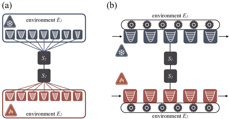
The situation becomes more involved when the system $S$ is made up of several interacting subsystems $S_{1},\ldots,S_{n}$ and each subsystem interacts with a local environment $E_{i}$, possibly held at different temperatures $T_{i}$ (see Fig. 1(a)). This type of scenario is the basis for the description of transport properties in quantum systems. Microscopic derivations in this case usually lead to global master equations (GMEs), in which the environment introduces jump operators that allow for incoherent excitation transfers between the different subsystems Rivas2010b; Purkayastha2016; Santos2016; Gonzalez2017; HoferNJP2017. However, these derivations are in general quite involved since they require knowledge of the full set of eigenvalues and eigenvectors of the system’s Hamiltonian, something which quickly becomes prohibitive when the number of subsystems increases. Moreover, depending on the approximations employed, one may also arrive at equations which do not generate completely positive maps (the so-called Redfield equations Purkayastha2016), or equations which contain unphysical heat currents Wichterich2007. For these reasons, microscopic derivations of master equations for systems connected to multiple environments still continues, nowadays, to be a topic of great interest.

An alternative, more heuristic, approach consists in deriving a master equation for the individual subsystems, neglecting the interaction with the remaining subsystems. The resulting master equation will then contain only local jump operators describing exchanges between the environment $E_{i}$ and its corresponding subsystem $S_{i}$. Such equations, which we shall henceforth refer to as local master equations (LME) (also frequently called boundary-driven master equations), are typically accurate when the dissipation rates are larger than the interaction between subsystems. Due to their computational simplicity, they have been extensively employed over the last two decades in the study of transport in non-equilibrium quantum systems Karevski2009; Karevski2013; Asadian2013; Landi2014b; Landi2015a; Schuab2016a; Guimar2016; Cui2015; Prosen2011b; Prosen2011; Prosen2008a; Prosen2012; Prosen2013a; NicacioPRE2015; CampbellSR2016; NicacioPRA2016; Ozgur1; Chanda; PereiraPRE2018.

Figure 1: We consider in this paper a system $S$ composed of several sub-systems $S_{1},\ldots,S_{N}$ (in the figure $N=2$). Each sub-system $S_{i}$ is connected to a local environment $E_{i}$ prepared in a different temperature $T_{i}$. (a) The standard bosonic heat bath model: the environment is assumed to consist of an ensemble of independent quantum harmonic oscillators with different frequencies in thermal equilibrium and coupled permanently to the system. (b) In this paper we focus instead on the framework of the repeated interactions method: the environment $E_{i}$ is divided into a series of ancillas (in this case represented by individual bosonic modes with identical frequencies) which interact with $S_{i}$ sequentially. This type of method leads to local master equations (LMEs), irrespective of the internal interactions between $S_{i}$ and $S_{j}$.

It turns out, however, that the nonlocal terms neglected in the LME may still lead to non-thermal steady states Cresser1992 and play a significant role if the heat exchanges are small, even for weakly interacting parts. As a consequence, it has been found that LMEs may lead to apparent thermodynamic inconsistencies, as pointed out recently by Levy and Kosloff LevyKosloffEPL2014. They have shown that the LME for two coupled quantum harmonic oscillators (QHO) may predict currents from a cold to a hot thermal reservoir, or the existence of currents even in the absence of a temperature gradient. Moreover, both may occur even in the limit of weakly coupled oscillators. The origin of these effects, as shown in LevyKosloffEPL2014, lies in the fact that the heat fluxes become of the same order of magnitude as the neglected nonlocal terms. They thus suggest to use the GME to fix such thermodynamic anomalies. These findings generated a considerable stream of investigations on the comparison between global and local master equations Rivas2010b; CorreaPRE2013; Guimar2016; Volovich; Gonzalez2017; HoferNJP2017; Stockburger2017; Decordi2017; MitchisonNJP2018; naseem2018thermodynamic; shammah2018open as well as clever possible alternatives Katz2016; SeahPRE2018.

Recent results indicate, however, that it is possible to construct a consistent thermodynamic framework for LMEs, resolving these seeming contradictions. First and foremost, it is important to mention that, unlike Redfield equations, LMEs are in Lindblad form and therefore generate completely positive trace preserving (CPTP) maps. Second, LMEs, being CPTP maps, can be microscopically derived in a controlled way using the idea of repeated interactions (collisional models) ScaraniPRL2002; ZimanPRA2002; Karevski2009; PalmaGiovannetti; Landi2014b; Barra2015; Strasberg2016; Manzano2016. In this approach, each environment is divided into an ensemble of identically prepared auxiliary systems, called units, which interact sequentially with an individual subsystem for a short time $\tau$ (see Fig. 1(b)). In the limit $\tau\to 0$ this leads to a LME, irrespective of the internal system interactions. Thirdly, Barra recently showed that since the interaction between the auxiliary units and the system is time dependent, there is an inherent external work required for generating the dissipative evolution described by the LME Barra2015. Hence, it is possible to put forth a consistent thermodynamic framework for the repeated interactions scheme, including definitions of heat, work and entropy production Barra2015; Strasberg2016.

The goal of this paper is to advance further on this reconciliation between LMEs and thermodynamics. Using the techniques of eigenoperators, we show that while LMEs satisfy local detailed balance, in general global detailed balance is broken. Moreover, we find that there is a fundamental work cost associated with this breaking of global detailed balance. By taking this exact work cost into account, we then show that LMEs become fully reconciled with thermodynamics. Quite surprisingly, the discrete nature of the repeated interactions method allows us to establish a direct mapping between non-equilibrium steady-states and limit-cycles of quantum heat engines. Hence, we find that the anomalous situation in which heat flows from cold to hot baths corresponds simply to a refrigerator, requiring positive injection of work to operate.

As our main application, we focus on the case of a system of two coupled quantum harmonic oscillators (QHO), which has been the subject of considerable interest due to potential applications in trapped ions Barreiro2011; Bermudez2013, optomechanical systems Ockeloen-Korppi2018; Brunelli2016a and ultra-cold atoms Brunelli2016a; Landig2016. Several interesting features of this model are studied in detail. First we show how to engineer the system to behave as a refrigerator, a heat engine or an accelerator. We study the efficiency and/or coefficient of performance for this model and show that they reach the optimal value of the Otto cycle in the case where the oscillators interact without counter-rotating terms in the Hamiltonian: including counter-rotating terms only degrades the operation of the system. We also discuss how to reconcile these results with a theorem by Martinez and Paz MartinezPaz, which states that no autonomous refrigeration is possible with equilibrium harmonic oscillators linearly coupled.

Let us mention that, given a physical system, the actual choice of whether to describe it using an LME or a GME approach depends ultimately on the system itself. Here we stress that the LME approach per se does not give rise to thermodynamic inconsistencies, provided the mechanism for its emergence is fully taken into account.

In order to clearly present the motivation behind our study and the main features of our approach, we begin in Sec. II with the simplest example of a LME, consisting of two coupled QHOs. We first review the seeming thermodynamic inconsistencies that may stem from this model and then go on to show how the results obtained using the method of repeated interactions can be used to completely remove them. Then, in Sec. III we carry out our main theoretical development, showing how the eigenoperator technique may be used to directly access thermodynamic quantities and describe the possible breaking of global detailed balance. Finally, in Sec. IV we return to the oscillator model and show how the full machinery of our approach may be employed to study the interplay between different types of interactions between the two oscillators. Finally, in Sec. V we summarise our results and conclude. Our paper also contains three appendices with various details of the derivations of our main results. In Appendix A we review the technique of Lyapunov equations for dealing with Gaussian continuous variable systems. In Appendix B we provide additional mathematical details on the developments of Sec. III. In Appendix LABEL:sec:prod we compute the entropy production showing that it is always positive.

II Steady-state of two harmonic oscillators subject to a local master equation

In order to motivate our study and provide an intuitive summary of our main results, we begin by discussing the model studied by Levy and Kosloff LevyKosloffEPL2014, consisting of two coupled harmonic oscillators, $S_{1}$ and $S_{2}$, each coupled to its own local heat bath via a LME (see Fig. 1(a)). The Hamiltonian is taken to be

$$H_{S}=H_{1}+H_{2}+H_{I},$$ (1)

where

$$H_{i}=\frac{1}{2}(p_{i}^{2}+\omega_{i}^{2}x_{i}^{2})=\omega_{i}(a_{i}^{\dagger}a_{i}+\nicefrac{{1}}{{2}}),$$ (2)

and

$$H_{I}=\epsilon(a^{\dagger}_{1}a_{2}+a_{1}a^{\dagger}_{2}).$$ (3)

Here $a_{i}$ are the annihilation operators of each harmonic oscillator and $(x_{i},p_{i})$ the corresponding position and momentum ($\hbar=k_{B}=1$). Both oscillators are assumed to have unit mass, but different frequencies $\omega_{i}$. The interaction (3) is taken to be of the typical tight-binding form, which conserves the number of quanta in the case of equal frequencies, $\omega_{1}=\omega_{2}$. More general interactions will be discussed in Sec. IV

The system is also subject to two baths $E_{1}$ and $E_{2}$, which we assume can be modeled by LMEs acting only on $S_{1}$ and $S_{2}$. Hence, we take the system to evolve according to the Lindblad master equation

$$\frac{\,\mathrm{d}\rho_{S}}{\,\mathrm{d}t}=-i[H_{S},\rho_{S}]+D_{1}(\rho_{S})+D_{2}(\rho_{S}),$$ (4)

where

$$D_{i}(\rho_{S})=\gamma(n_{i}+1)\mathcal{L}[a_{i},\rho]+\gamma n_{i}\mathcal{L}[a^{\dagger}_{i},\rho].$$ (5)

Here $\gamma$ is the dissipation rate, $n_{i}$ is the average excitation number for the Bose-Einstein distribution,

$$n_{i}=\frac{1}{e^{\beta_{i}\omega_{i}}-1},$$ (6)

with inverse temperature $\beta_{i}=(T_{i})^{-1}$ and

$$\mathcal{L}[A,\rho]=A\rho A^{\dagger}-\frac{1}{2}\{A^{\dagger}A,\rho\},$$ (7)

is the dissipator in Lindblad form. Henceforth, we always assume that $T_{1}<T_{2}$ (see Fig. 1(a)). Below, it will also be useful to keep in mind that $n_{i}$ is a monotonically increasing function of $T_{i}/\omega_{i}$.

II.1 Predictions for the steady-state

Due to the form of the Hamiltonian and the jump operators, the steady-state of the master equation (4) will be Gaussian and can therefore be easily found using the standard Lyapunov equation technique. A review of this method is given for completeness in Appendix A. Here we only focus on the main results, which can be summarized by the following expectation values: rCl ⟨a_1^†a_1 ⟩&= n_1 + 2ϵ2Δ2 (n_2 - n_1),
⟨a_2^†a_2 ⟩= n_2 - 2ϵ2Δ2 (n_2 - n_1),
⟨a_2^†a_1 ⟩= ϵΔ2(ω_1 - ω_2 + i γ)(n_1 - n_2). where $\Delta^{2}=\gamma^{2}+4\epsilon^{2}+(\omega_{1}-\omega_{2})^{2}$. Using Eq. (2) we then find that the energy of oscillator 1 will be

$$\langle H_{1}\rangle=\langle H_{1}\rangle_{\text{th}}+\frac{2\omega_{1}\epsilon^{2}}{\Delta^{2}}(n_{2}-n_{1}),$$ (8)

where $\langle H_{1}\rangle_{\text{th}}=\omega_{1}(n_{1}+\nicefrac{{1}}{{2}})$ is the energy the oscillator would have if it were in thermal equilibrium with its corresponding bath. An equivalent expression can be obtained for the second oscillator replacing $1\leftrightarrow 2$. Similarly, the heat flux from the first oscillator to the second will be

$$\dot{Q}_{1\to 2}=-i\left\langle[H_{S},H_{1}]\right\rangle=-i\omega_{1}\epsilon\langle a^{\dagger}_{1}a_{2}-a_{1}a^{\dagger}_{2}\rangle=\frac{2\gamma\epsilon^{2}\omega_{1}}{\Delta^{2}}(n_{2}-n_{1}),$$ (9)

which is consistent with the expression obtained in Ref. LevyKosloffEPL2014.

The relevant point to highlight from these results is that the sign of the $\epsilon^{2}$-terms in Eqs. (8) and (9) will depend on the relative magnitudes of $n_{1}$ and $n_{2}$ and not of $T_{1}$ and $T_{2}$. This simple fact, when combined with the definition of $n_{i}$ in Eq. (6), introduces several properties which, at first sight, seem to violate the second law of thermodynamics. First, it implies that oscillator 1 can be cooled to a temperature smaller than the temperature $T_{1}$ of the coldest reservoir, in the sense that it could reach a state with lower energy than that of the thermal state it would reach if it were in contact only with the coldest reservoir. Second, one may obtain a non-zero heat current even if both baths are at the same temperature, $T_{1}=T_{2}$. And third, if $T_{1}<T_{2}$ but we happen to satisfy

$$n_{1}>n_{2}\quad\leftrightarrow\quad\frac{T_{1}}{\omega_{1}}>\frac{T_{2}}{\omega_{2}},$$ (10)

then there will be a current flowing from the cold to the hot bath ($\dot{Q}_{1\to 2}<0$).

As pointed out in Ref. LevyKosloffEPL2014, these results seem to violate the second law of thermodynamics, a fact which the authors attribute to the inadequacy of local master equations to describe transport processes. The result of the cooling of the first oscillator below the temperature of the coldest environment also seems to suggest that this master equation could be used to design Gaussian (quadratic) absorption refrigerators, which would contradict a general theorem proved by Martinez and Paz MartinezPaz.

Table 1: The three modes of operation of the steady-state of the two oscillators, always assuming $E_{1}$ is the cold reservoir ($T_{1}<T_{2}$). In this paper positive heat or work always means energy entering the system. So $\dot{Q}_{i}>0$ means energy entered $S$ through $E_{i}$ and $\dot{W}_{\rm ext}>0$ means work was performed on the system by an external agent.

Mode of operation		$\dot{Q}_{1}$	$\dot{Q}_{2}$	$\dot{W}$	Operation regime
Refrigerator		$\dot{Q}_{1}>0$	$\dot{Q}_{2}<0$	$\dot{W}>0$	$\omega_{1}<\omega_{2}T_{1}/T_{2}$
Consumes work to make heat flow from cold to hot.
Engine		$\dot{Q}_{1}<0$	$\dot{Q}_{2}>0$	$\dot{W}<0$	$\omega_{2}T_{1}/T_{2}<\omega_{1}<\omega_{2}$
Uses hot bath to produce useful work, dumping the remainder in the cold bath.
Accelerator (oven)		$\dot{Q}_{1}<0$	$\dot{Q}_{2}>0$	$\dot{W}>0$	$\omega_{1}>\omega_{2}$
Consumes work to heat the cold reservoir more than it would with spontaneous thermal conduction.

II.2 Resolving the thermodynamic inconsistencies

Using Eq. (4) one finds that the total rate of change of the system Hamiltonian (1) is given by rCl d⟨HS⟩dt &= γ(n_1 - ⟨a_1^†a_1 ⟩) + γ(n_2 - ⟨a_2^†a_2 ⟩)
- γϵ⟨a_1^†a_2 + a_2^†a_1 ⟩. However, this change in energy cannot be associated only with heat flowing to the reservoirs Barra2015. Instead, there is an associated work cost which, as we show below, is related to the breaking of global detailed balance. Quoting the results that will be derived in Sec. III, we now discuss how one can remove all the inconsistencies by including this work cost.

In particular, we find that the correct splitting of Eq. (II.2) is of the form

$$\frac{\,\mathrm{d}\langle H_{S}\rangle}{\,\mathrm{d}t}=\dot{Q}_{1}+\dot{Q}_{2}+\dot{W}_{\rm ext},$$ (11)

where

$$\dot{Q}_{i}={\rm tr}\left[D_{i}(\rho_{S})H_{i}\right]=\gamma\omega_{i}(n_{i}-\langle a_{i}^{\dagger}a_{i}\rangle),$$ (12)

is the heat rate flowing from each reservoir to the system (see Eq. (31) for the general expression) and

$$\dot{W}_{\rm ext}={\rm tr}\left\{\left[D_{1}(\rho_{S})+D_{2}(\rho_{S})\right]H_{I}\right\}=-\gamma\epsilon\langle a_{1}^{\dagger}a_{2}+a_{2}^{\dagger}a_{1}\rangle.$$ (13)

is the required work rate (see Eq. (33) for the general expression). From Eqs. (II.1)-(II.1) we then find that in the steady-state rCl ˙Q_1 &= 2γϵ2Δ2ω_1(n_1-n_2),
˙Q_2 = -2γϵ2Δ2ω_2(n_1-n_2),
˙W_ext = -2γϵ2Δ2 (ω_1 - ω_2)(n_1 - n_2).

These are very important results, which we shall now discuss in depth. But before doing so, some consistency checks are in order. First, $\dot{W}_{\rm ext}$ tends to zero as $\epsilon\to 0$, in which case global detailed balance is recovered. Second, the work required is proportional to $\gamma\epsilon^{2}$. As discussed in Ref. Gonzalez2017, the local master equation can be shown to be correct for small interactions $\epsilon$ up to the same order (see comment in Sec. II D in that paper). Third, in the steady-state $\,\mathrm{d}\langle H_{S}\rangle/\,\mathrm{d}t=0$ so that we should have

$$\dot{W}_{\rm ext}=-\dot{Q}_{1}-\dot{Q}_{2},$$ (14)

as can indeed be easily verified.

Figure 2: The three regimes of operation in Table 1, for the steady-state of two harmonic oscillators. (a)-(c) $\dot{Q}_{1}$, $\dot{Q}_{2}$ and $\dot{W}_{\rm ext}$, Eqs. (13)-(13), as a function of $\omega_{1}/\omega_{2}$. (d) $\dot{Q}_{1}/\dot{W}_{\rm ext}$, which follows precisely the Otto value $\omega_{1}/(\omega_{2}-\omega_{1})$. (e) $\dot{W}_{\rm ext}/\dot{Q}_{2}$ which also follows the Otto value $\omega_{1}/\omega_{2}-1$. All curves are plotted for $\gamma\epsilon^{2}/\Delta^{2}=\omega_{2}$, assuming $T_{1}/T_{2}=1/2$. The vertical lines represent $\omega_{1}/\omega_{2}=T_{1}/T_{2}$ and $\omega_{1}=\omega_{2}$.

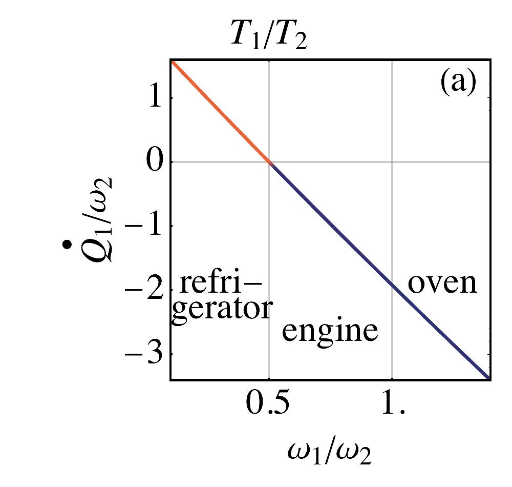
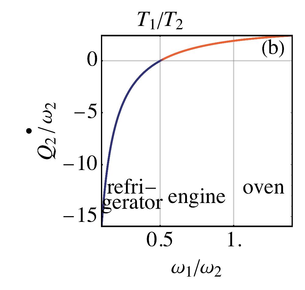
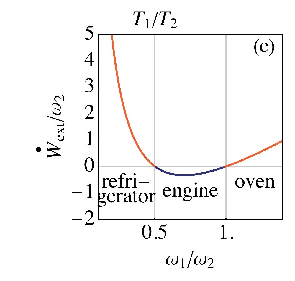
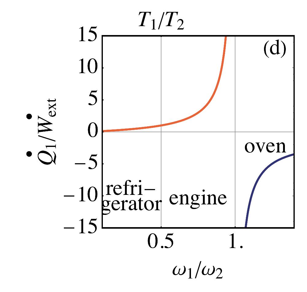
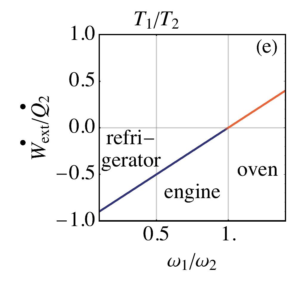
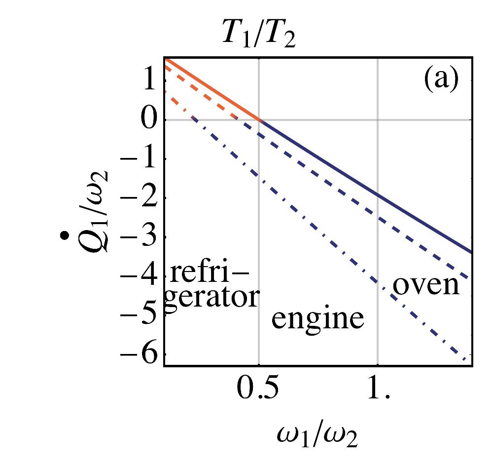
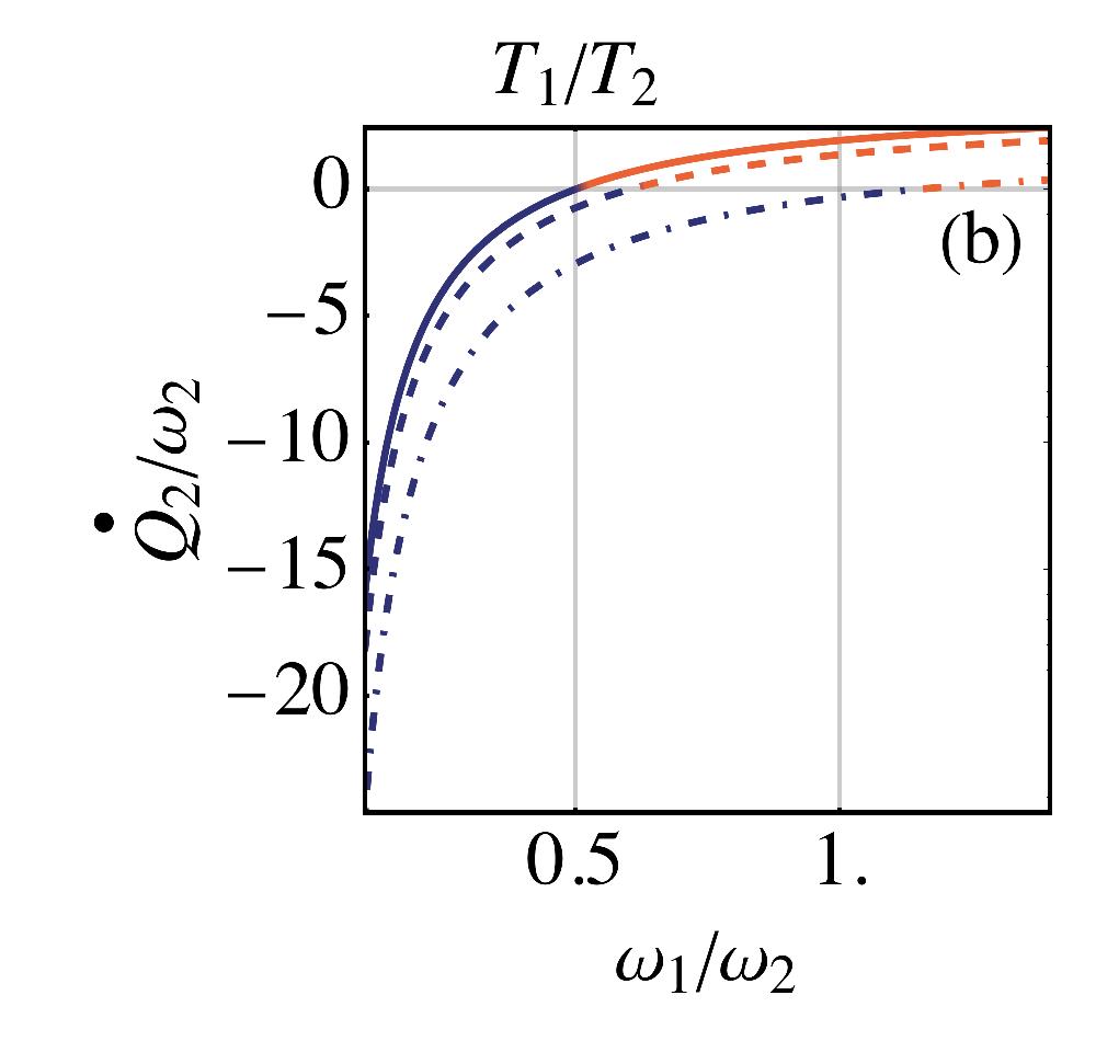
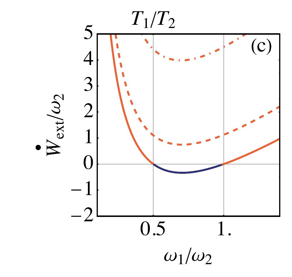
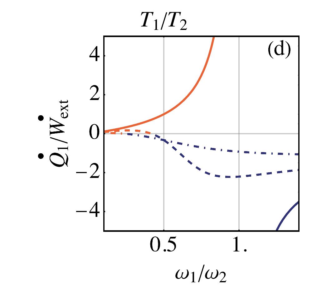
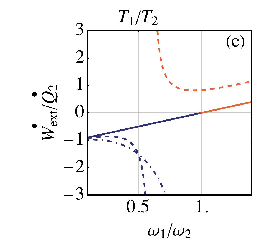
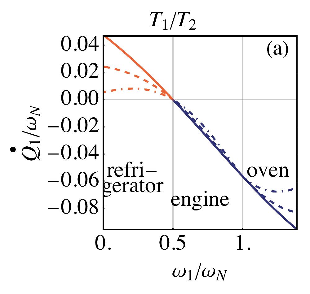
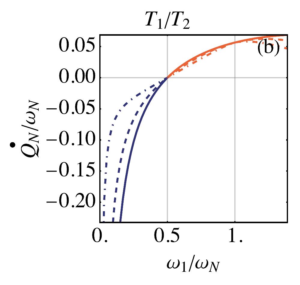
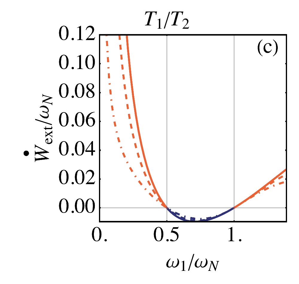
We now show that, once this work cost is correctly attributed, the two-oscillator system at steady-state functions precisely as a heat engine, with two reservoirs and a work source. Indeed, we find from Eqs. (13)-(13) that the system can be tuned to function as a refrigerator, a thermal engine or an accelerator (oven). The description of each mode of operation and what they mean in terms of $\dot{Q}_{1}$, $\dot{Q}_{2}$ and $\dot{W}$ is presented in Table 1. We also show in Fig. 2 a plot of these 3 quantities illustrating the typical operation regimes.

We begin with the case of a refrigerator, $\dot{Q}_{1}>0$. According to Eq. (13), this requires $n_{1}>n_{2}$ which is tantamount to the condition (10). But we now see that when this condition is satisfied, one also has $\dot{W}_{\rm ext}>0$. Thus, for the two oscillators to act as a refrigerator, they must absorb work from an external agent. Hence, we see that there are no violations of the second law. Instead, by taking into account this work cost, one recovers a fully consistent thermodynamic description. The coefficient of performance (COP) of the refrigerator is the ratio of the heat extracted from the cold environment divided by the work invested:

$${\rm COP}=\frac{\dot{Q}_{1}}{\dot{W}_{\rm ext}}=\frac{\omega_{1}}{\omega_{2}-\omega_{1}}$$ (15)

which coincides with the COP of the Otto cycle. As will become clear in Sec. III, this connection between a steady-state and the limit-cycle of a heat engine, can actually be traced back to the basic idea of the repeated interactions method, which models the steady-state as a sequence of (extremely short) strokes, each having an associated work rate and heat rate. Notwithstanding, we should also mention that an Otto COP is a special consequence of this type of interaction. As will be shown in Sec. IV, the introduction of counter-rotating terms only reduces the COP below the Otto value.

Increasing $\omega_{1}$ in the interval

$$\frac{T_{1}}{T_{2}}\omega_{2}<\omega_{1}<\omega_{2},$$ (16)

we find that the two-oscillator system in its steady-state functions as a thermal machine, extracting heat from the hot bath, producing work and dumping heat in the cold bath. In this regime the machine’s efficiency will be:

$$\eta=\frac{|\dot{W}_{\rm ext}|}{\dot{Q}_{2}}=1-\frac{\omega_{1}}{\omega_{2}}$$ (17)

which is again the Otto efficiency for a thermal machine. Finally, for $\omega_{2}<\omega_{1}$ we necessarily have $n_{1}<n_{2}$ and therefore $\dot{Q}_{1}<0$, $\dot{Q}_{2}>0$ and $\dot{W}_{\rm ext}>0$. Thus the device transports heat from the hot to the cold environment and at the same time transforms work into heat which is damped in the cold bath: $|\dot{Q}_{1}|=\dot{W}_{\rm ext}+\dot{Q}_{2}>\dot{Q}_{2}$. Hence, it functions as an accelerator (i.e. an oven) Buffoni2018, heating the cold reservoir faster than it would with spontaneous thermal conduction.

Notice that at the special value $\omega_{1}/\omega_{2}=T_{1}/T_{2}$, the system operates as a thermal machine with the Carnot efficiency and zero power.

We conclude this section by emphasising that within the repeated interactions framework one is able to resolve all of the seeming thermodynamic inconsistencies of local master equations. The zeroth law does not apply since the system is externally driven. The first law is satisfied, as we accounted for the energy balance of the whole system plus environment, including the required work cost. The second law is satisfied, as refrigeration is not spontaneous, but accompanied by external work. And finally, the LMEs do not violate the theorem by Martinez and Paz MartinezPaz, which states that no autonomous refrigeration is possible with equilibrium harmonic oscillators. In fact, in our framework, there is also work associated with the environment-system interaction so the machine is not autonomous.

We now move on to the mathematical development of LMEs using eigenoperators and the repeated interactions.

III The method of repeated interactions

We now turn to the microscopic derivation of LMEs using the method of repeated interactions ScaraniPRL2002; ZimanPRA2002; Karevski2009; PalmaGiovannetti; CiccarelloPRA2013; LorenzoPRA2015; Landi2014b; LorenzoPRL2015; Barra2015; Strasberg2016; Manzano2016; Ciccarello2017; PezzuttoNJP2016; pezzutto2018out; cusumano2018entropy; CampbellPRA2018; GrossQST2018, which will form the basis for our thermodynamic description. The basic idea behind the method of repeated interactions is to model the environment as a set of units, each prepared in a thermal state. At time $t=0$ the system $S$ is allowed to interact for a certain time $\tau$ with one such unit, which we generically refer to as $E$. After this time the unit is discarded and a fresh new one is introduced, again in the same initial state. The process is then repeated sequentially. For $\tau\to 0$ this method generates a continuous time description which can be modelled by a Lindblad master equation that is, in general, local. We emphasise that a larger class of non-Markovian master equations including the global master equation can be engineered in a similar way PalmaGiovannetti and realised experimentally as proposed in Ref. JinPRA2015.

We consider here this method implemented in the general scenario of Fig. 1(b) and derive the results of the previous section as particular cases. Our system $S$ is therefore assumed to be composed of $N$ subsystems $S_{1},\ldots,S_{N}$, where each $S_{i}$ interacts with its own environment $E_{i}$. The Hamiltonian of the system is taken to be

$$H_{S}=\sum\limits_{i=1}^{N}H_{S_{i}}+H_{I},$$ (18)

where $H_{S_{i}}$ is the Hamiltonian of subsystem $S_{i}$ and $H_{I}$ summarises all interactions between subsystems. Moreover, the total Hamiltonian comprising the system, the environments and all interactions, is taken as

$$H_{\text{tot}}=H_{S}+\sum\limits_{i=1}^{N}H_{E_{i}}+\frac{1}{\sqrt{\tau}}\sum\limits_{i=1}^{N}V_{i},$$ (19)

where $H_{E_{i}}$ is the Hamiltonian of environment $E_{i}$ and $V_{i}$ is the interaction between $S_{i}$ and $E_{i}$. We also follow the customary approach of scaling the $V_{i}$ by the interaction time $\tau$, which is convenient, although not necessary, for taking the continuous time limit Landi2014b; Barra2015; Strasberg2016. Following the usual repeated interactions approach, the reduced density matrix of the system $\rho_{S}(t)$ will then evolve according to the map

$$\rho_{S}((n+1)\tau)=\operatorname{tr}_{E}\bigg{\{}e^{-i\tau H_{\text{tot}}}\;\rho_{S}(n\tau)\rho_{E}\;e^{i\tau H_{\text{tot}}}\bigg{\}},$$ (20)

where

$$\rho_{E}=\bigotimes\limits_{i=1}^{N}\frac{e^{-\beta_{i}H_{E_{i}}}}{\operatorname{tr}e^{-\beta_{i}H_{E_{i}}}},$$ (21)

is the thermal state of the environments.

Expanding Eq. (20) in a power series in $\tau$ one then finds, up to first order, the LME,

$$\frac{\,\mathrm{d}\rho_{S}}{\,\mathrm{d}t}=-i[H_{S},\rho_{S}]+\sum\limits_{i=1}^{N}D_{i}(\rho_{S}),$$ (22)

where $H_{S}$ is given in (18) and

$$D_{i}(\rho_{S})=-\frac{1}{2}\operatorname{tr}_{E_{i}}[V_{i},[V_{i},\rho_{S}\rho_{E_{i}}]].$$ (23)

The interesting aspect of this approach is that the structure of the dissipative terms are completely independent on the choice of $H_{S}$. Or, more specifically, on the interaction terms $H_{I}$. This is a consequence of the short interaction times between the system and environment which do not allow for the information of each $E_{i}$ to scramble towards different $S_{j}$ Campisi2017a; Garttner2017.

III.1 Local vs. Global detailed balance

Up to now the discussion makes no reference to the structure of the system-environment interactions $V_{i}$. A particularly interesting situation, which is in practice the most widely studied case, is when the $V_{i}$ satisfy local detailed balance with respect to each subsystem, but do not necessarily satisfy global detailed balance due the system-system interactions $H_{I}$. To make this argument more precise we introduce the idea of eigenoperators.

By using the method of eigenoperators, we can cast the conditions of detailed balance in terms solely of the algebra of operators. This therefore allows us to introduce the notion of local vs. global detailed balance, as referring to the local or global Hamiltonian of the system. We note that here this terminology is being used in a slightly different context as, for instance, Ref. Barra2015. There the term is employed in the standard sense of “detailed balance” KatzPRB1983.

Let $H$ be an arbitrary Hamiltonian. An operator $A$ is called an eigenoperator of $H$ if it satisfies $[H,A]=-\omega A$, for some $\omega>0$ (usually referred to as a Bohr, or transition, frequency). Due to this algebra, $A$ and $A^{\dagger}$ function as lowering and raising operators for the $H$, causing transitions between energy levels $E$ and $E^{\prime}$ separated by an energy $\omega$.

Returning to our problem, we shall assume that the $V_{i}$ have the form

$$V_{i}=\sum\limits_{k}g_{i,k}(L_{i,k}^{\dagger}A_{i,k}+L_{i,k}A_{i,k}^{\dagger}),$$ (24)

where $g_{i,k}$ are constants, while $L_{i,k}$ and $A_{i,k}$ are eigenoperators of $H_{S_{i}}$ and $H_{E_{i}}$ respectively. That is: rCl [H_S_i, L_i,k] = - ω_i,k L_i,k,
[H_E_i, A_i,k] = - ω_i,k A_i,k, where, for each $S_{i}$, $\{\omega_{i,k}\}$ represents the set of transition frequencies of the Hamiltonian $H_{S_{i}}$. The rationale behind these expressions is the following. For each subsystem $S_{i}$, the set of Bohr frequencies $\{\omega_{i,k}\}$ can be viewed as the set of transitions which are activated in that subsystem, due to the contact with its local bath. For instance, in the case of a harmonic oscillator, a dissipator such as (5) is characterized by an eigenoperator $a$, which only induces transitions between neighboring levels. Hence, the only Bohr frequency would be $\omega$ (the natural frequency of the oscillator). Similarly, a system-environment interaction containing $a^{2}$ would induce transitions with Bohr frequencies $2\omega$.

In an interaction such as (24), however, there is also the additional assumption that whenever there is a transition of $+\omega_{i,k}$ in the system, the corresponding transition in $E_{i}$ occurs with energy $-\omega_{i,k}$ Hence, it follows that

$$[H_{S_{i}}+H_{E_{i}},V_{i}]=0,$$ (25)

meaning that all the energy that leaves system $S_{i}$ enters bath $E_{i}$. This equation, together with the assumption that the bath is thermal, implies local detailed balance.

However, a similar relation does not hold for the total system Hamiltonian $H_{S}$, due to the interaction $H_{I}$ between subsystems. The reason is that, in general, $L_{i,k}$ are not eigenoperators of $H_{I}$. Hence,

$$[H_{S}+H_{E},V]=[H_{I},V]\neq 0,$$ (26)

where $H_{E}=\sum_{i=1}^{N}H_{E_{i}}$ and $V=\sum_{i=1}^{N}V_{i}$. This means that even though detailed balance may hold locally, it is violated globally. As will be shown below, taking into account this fact is essential for providing a consistent thermodynamic description of LMEs.

Substituting Eq. (24) in Eq. (23) one may obtain a more explicit formula for the LME dissipators. To do so one notices that since the environments are in equilibrium, it follows that $\langle A_{i,k}A_{i,q}\rangle=0$ and $\langle A_{i,k}^{\dagger}A_{i,q}\rangle\propto\delta_{k,q}$. Hence, Eq. (23) reduces to

$$D_{i}(\rho_{S})=\sum\limits_{k}\gamma_{i,k}^{-}\;\mathcal{L}[L_{i,k},\rho_{S}]+\gamma_{i,k}^{+}\;\mathcal{L}[L_{i,k}^{\dagger},\rho_{S}]$$ (27)

where $\mathcal{L}[A,\rho]$ is the Lindblad dissipator defined in Eq. (7), whereas rCl γ_i,k^- &= g_i,k^2   ⟨A_i,k A_i,k^†⟩,

γ_i,k^+ = g_i,k^2   ⟨A_i,k^†A_i,k ⟩. Since the $A_{i,k}$ are eigenoperators of the bath which is in equilibrium at inverse temperature $\beta_{i}$, it follows that

$$\frac{\gamma_{i,k}^{+}}{\gamma_{i,k}^{-}}=e^{-\beta_{i}\omega_{i,k}},$$ (28)

which is another manifestation of local detailed balance.

III.2 Example: two harmonic oscillators

To show how these results may be applied, we consider again the two harmonic oscillators $a_{1}$ and $a_{2}$ treated in Sec. II. We assume that the environmental units $E_{1}$ and $E_{2}$ are themselves harmonic oscillators with operators $b_{1}$ and $b_{2}$  , and we take the total Hamiltonian to be

$$H_{\text{tot}}=H_{S}+\sum\limits_{i=1,2}\bigg{\{}\omega_{i}b_{i}^{\dagger}b_{i}+g(a_{i}^{\dagger}b_{i}+b_{i}^{\dagger}a_{i})\bigg{\}},$$ (29)

where $H_{S}$ is given in Eq (1). Since the frequency $\omega_{1}$ of $S_{1}$ and $E_{1}$ are the same, the operators $a_{1}$ and $b_{1}$ are eigenoperators of $H_{1}=\omega_{1}a_{1}^{\dagger}a_{1}$ and $H_{E_{1}}=\omega_{1}b_{1}^{\dagger}b_{1}$. Hence, local detailed balance, Eq. (25), is satisfied. However, $a_{1}$ is not an eigenoperator of $H_{S}$ due to the interaction term $H_{I}=\epsilon(a_{1}^{\dagger}a_{2}+a_{1}a_{2}^{\dagger})$ [Eq. (3)] so that global detailed balance is in general broken.

Applying Eq. (27) with $L_{i,k}=a_{i}$ and $A_{i,k}=b_{i}$ we then immediately find the master equation (4) with the transition rates $\gamma_{i,k}^{\pm}$ given by

$$\gamma_{i}^{+}=g^{2}\langle b_{i}^{\dagger}b_{i}\rangle:=\gamma n_{i},\qquad\gamma_{i}^{-}=g^{2}\langle b_{i}b_{i}^{\dagger}\rangle=\gamma(n_{i}+1).$$ (30)

which are the coefficients in Eq. (5).

III.3 Thermodynamics of the repeated interactions method

We now turn to a description of the thermodynamics of the repeated interactions method. Since the global S+E interaction is unitary, we may study the changes in the energy of the system and environment individually for a given stroke. The heat $\delta Q_{i}$ exchanged between the system and environment $i$ in one stroke must then be simply $\langle H_{E_{i}}\rangle_{0}-\langle H_{E_{i}}\rangle_{\tau}$. Dividing by $\tau$ and taking the limit $\tau\to 0$ will give the heat current $\dot{Q}_{i}$ to environment $E_{i}$. The explicit calculation is postponed to Appendix B. As a result, we find the surprisingly simple formula:

$$\dot{Q}_{i}=\sum\limits_{k}\omega_{i,k}\bigg{\{}\gamma_{i,k}^{+}\langle L_{i,k}L_{i,k}^{\dagger}\rangle-\gamma_{i,k}^{-}\langle L_{i,k}^{\dagger}L_{i,k}\rangle\bigg{\}}.$$ (31)

For example, in the case of the two harmonic oscillators, Eq. (31) gives precisely the heat-rate formula (12) that was used in Sec. II.

In addition to the heat rates, however, there will in general also be a work contribution. The simplest way of seeing this is to note that for each interaction stroke one must turn the system-environment coupling on and off, so that the total Hamiltonian (19) must actually be time-dependent. Since the global S-E system is isolated, the work in an individual stroke between times $n\tau$ and $(n+1)\tau$ may be unambiguously defined as

$$\delta W_{\rm ext}=\int\limits_{n\tau}^{(n+1)\tau}\left\langle\frac{\partial H_{\text{tot}}}{\partial t}\right\rangle\,\mathrm{d}t.$$ (32)

Again, dividing by $\tau$ and taking the limit $\tau\to 0$ yields the work rate $\dot{W}_{\rm ext}$. As shown in Appendix B, carrying out this computation yields

$$\dot{W}_{\rm ext}=\frac{1}{2}\sum\limits_{i,k}\bigg{\{}\gamma_{i,k}^{-}\langle L_{i,k}^{\dagger}F_{i,k}\rangle-\gamma_{i,k}^{+}\langle F_{i,k}L_{i,k}^{\dagger}\rangle\bigg{\}}+\text{c.c.},$$ (33)

where $F_{i,k}=[H_{I},L_{i,k}]$ and c.c. stands for complex conjugate. Hence, we see that the work rate is related precisely to the non-commutativity of the jump operators $L_{i,k}$ with the system-system interaction $H_{I}$. If global detailed balance, Eq. (26), is recovered, then the work cost is identically zero. Otherwise, whenever global detailed balance is broken, there will be an associated work cost. As an example, in the case of the two QHOs, $[H_{I},a_{1}]=-\epsilon a_{2}$, so that a direct application of Eq. (33) leads to expression (13).

From a practical point of view, Eqs. (31) and (33) are our main results, as they offer general expressions that may be applied over a broad range of situations. These results generalise Barra’s findings Barra2015 to arbitrary bath and system’s structure. In Appendix LABEL:sec:prod, we calculate the entropy production showing that it is indeed always positive in agreement with the second law. We now return to the problem of coupled harmonic oscillators and show how they can be applied to the study of more complex situations.

Figure 3: Similar to Fig. 2, but examining the influence of the counter-rotating term $\eta$ in the Hamiltonian (34). The solid curves are the same as Fig. 2. The dashed curves correspond to Eqs. (37)-(IV.1) for $\eta=0.3\omega_{2}$ (dashed) and $\eta=0.6\omega_{2}$ (dot-dashed). The curves were plotted for $\epsilon^{2}/\gamma=\omega_{2}$, assuming $T_{1}/T_{2}=1/2$. The vertical lines correspond to $\omega_{1}/\omega_{2}=T_{1}/T_{2}$ and $\omega_{1}=\omega_{2}$.

IV Quantum Harmonic Oscillators

We consider once again the problem studied in Sec. II, but we now make the following generalizations. First, we assume to have a one-dimensional chain of $N$, instead of 2, oscillators, with the first and last coupled to local baths. Second, we consider a more general type of interaction between them, so that we take the system Hamiltonian to be

$$H_{S}=\sum\limits_{i=1}^{N}\omega_{i}a_{i}^{\dagger}a_{i}+\sum\limits_{i=1}^{N-1}\bigg{\{}\epsilon(a_{i}^{\dagger}a_{i+1}+a_{i+1}^{\dagger}a_{i})+\eta(a_{i}^{\dagger}a_{i+1}^{\dagger}+a_{i+1}a_{i})\bigg{\}}$$ (34)

When $\eta=0$ we recover the excitation-conserving tight-binding model. Conversely, $\eta=\epsilon$ corresponds to a position-position coupling $x_{i}x_{i+1}$. The total system evolves according to the master equation

$$\frac{\,\mathrm{d}\rho_{S}}{\,\mathrm{d}t}=-i[H_{S},\rho_{S}]+D_{1}(\rho_{S})+D_{N}(\rho_{S}),$$ (35)

where $D_{i}(\rho_{S})$ is given in Eq (5).

Using Eq. (31) we find that the heat rate to the first and last environments will be

$$\dot{Q}_{i}=\gamma\omega_{i}(n_{i}-\langle a_{i}^{\dagger}a_{i}\rangle),\qquad i=1,N.$$ (36)

The work rate, on the other hand, is found using Eq. (33) and reads rCl ˙W &= γϵ2 ⟨a_1^†a_2 + a_1 a_2^†+ a_N^†a_N-1 + a_N a_N-1^†⟩
+ γη2 ⟨a_1 a_2 + a_1 a_2 + a_N a_N-1 + a_N a_N-1 ⟩. If $N=2$ and $\eta=0$ this reduces to Eq. (13).

IV.1 Degradation of the engine’s operation due to counter-rotating terms

As a first application, we return to the case of $N=2$ oscillators but generalize the results of Sec. II to include the counter-rotating terms $\eta$. We then show that, interpreting our steady-state as a heat engine, as in Fig. 2, the presence of this term only degrades the machine’s operation. We once again use the Lyapunov equation technique of Appendix A. Although the steady-state may be trivially found numerically, it turns out that the analytical expression for the covariance matrix becomes extremely cumbersome when $\eta\neq 0$. For the purpose of illustration, we therefore present here results that are valid when the bath coupling $\gamma$ is much larger than all other energy scales in the problem. In this case we find the following simple expressions for the heat rates (36) and the work rate (36):

$$\dot{Q}_{1} = \frac{2\omega_{1}}{\gamma}\bigg{[}\epsilon^{2}(n_{1}-n_{2})-\eta^{2}(n_{1}+n_{2}+1)\bigg{]},$$ (37)

$$\dot{Q}_{2} = -\frac{2\omega_{2}}{\gamma}\bigg{[}\epsilon^{2}(n_{1}-n_{2})+\eta^{2}(n_{1}+n_{2}+1)\bigg{]},$$ (38)

$$\dot{W}_{\rm ext} = -\frac{2}{\gamma}\bigg{[}\epsilon^{2}(n_{1}-n_{2})(\omega_{1}-\omega_{2})+$$

$$- \eta^{2}(\omega_{1}+\omega_{2})(n_{1}+n_{2}+1)\bigg{]}.$$

If $\eta=0$ we recover Eqs. (13)-(13), provided we also approximate $\Delta\simeq\gamma$.

The influence of $\eta$ in these thermodynamic quantities is shown in Fig. 3, which compares the results with those of Fig. 2 corresponding to $\eta=0$. As can be seen, the region in which the machine operates as a refrigerator or an engine is severely reduced by the presence of $\eta$. Moreover, as can be easily verified from Eqs. (37)-(IV.1), in the case $\eta=\epsilon$ of a position-position coupling all of these operation regimes become inaccessible. This type of behavior has already been observed experimentally in the case of opto-mechanical systems, in which the interplay between $\eta$ and $\epsilon$ can be tuned by appropriately choosing the pump’s sideband. And indeed, what is observed, is that since the $\eta$ interaction tends to entangle the two oscillators (since it leads to an evolution described by a two-mode squeezing operator), it has the general tendency of heating them up Wang2013; Woolley2014; Ockeloen-Korppi2018, which is precisely what is observed in Fig. 3.

IV.2 Analysis for a chain of $N$ oscillators

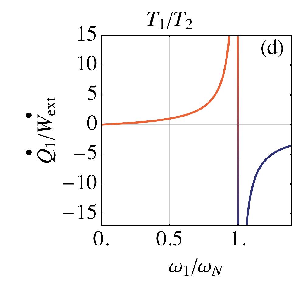
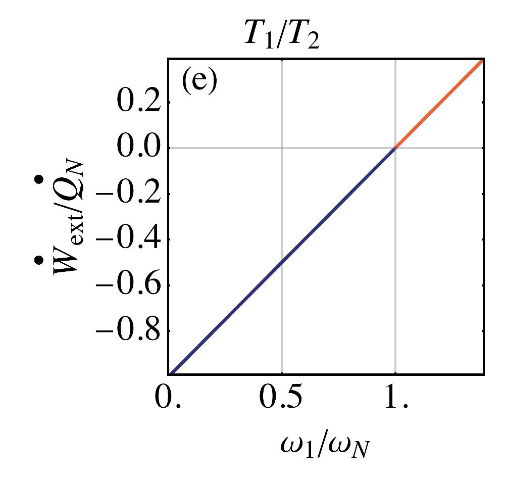
We next carry on a numerical analysis for the case of a chain of $N$ oscillators, assuming for simplicity that $\eta=0$. The steady-state in this case is obtained by solving the Lyapunov equation numerically (Appendix A). A set of results is presented in Fig. 4 for the case of a linear function profile

$$\omega_{i}=\frac{(N-i)\omega_{1}+(i-1)\omega_{N}}{N-1}.$$ (40)

As can be seen, in general the thermodynamic quantities depend on the system size. However, the ratios between heat and work are independent of size and only depend on the frequencies $\omega_{1}$ and $\omega_{N}$ of the initial and final oscillators. This can be proven rigorously after writing the continuity equation for the number of excitations of each oscillator using techniques similar to those employed in Ref. Asadian2013; Landi2014b:

$$\frac{d\langle a^{\dagger}_{1}a_{1}\rangle}{dt} = -i\epsilon\langle a^{\dagger}_{1}a_{2}-a_{1}a^{\dagger}_{2}\rangle+\gamma\left(n_{1}-\langle a^{\dagger}_{1}a_{1}\rangle\right),$$ (41)

$$\frac{d\langle a^{\dagger}_{i}a_{i}\rangle}{dt} = -i\epsilon\langle a^{\dagger}_{i}a_{i+1}-a_{i}a^{\dagger}_{i+1}\rangle,\quad i=2,\dots,N-1$$ (42)

$$\frac{d\langle a^{\dagger}_{N}a_{N}\rangle}{dt} = i\epsilon\langle a^{\dagger}_{N-1}a_{N}-a_{N-1}a^{\dagger}_{N}\rangle+\gamma\left(n_{N}-\langle a^{\dagger}_{N}a_{N}\rangle\right).$$ (43)

Hence, at steady state we have:

$$\gamma\left(n_{1}-\langle a^{\dagger}_{1}a_{1}\rangle\right)=-\gamma\left(n_{N}-\langle a^{\dagger}_{N}a_{N}\rangle\right)$$ (44)

and replacing this in the expressions for the heat flows (36) we obtain:

$$\dot{Q}_{1}=\gamma\omega_{1}\left(n_{1}-\langle a^{\dagger}_{1}a_{1}\rangle\right)=-\frac{\omega_{1}}{\omega_{N}}\dot{Q}_{N}.$$ (45)

Finally, using the first law of thermodynamics: $\dot{W}_{\rm ext}+\dot{Q}_{1}+\dot{Q}_{N}=0$ we obtain:

$$\frac{\dot{Q}_{1}}{\dot{W}_{\rm ext}}=\frac{\omega_{1}}{\omega_{N}-\omega_{1}};\quad\frac{\dot{W}_{\rm ext}}{\dot{Q}_{N}}=-1+\frac{\omega_{1}}{\omega_{N}}.$$ (46)

We remark that these ratios coincide with those of Otto thermal machines and refrigerators operating with a single harmonic oscillator driven between frequencies $\omega_{1}$ and $\omega_{N}$. Moreover, the universal ratios (46) would hold if we replace the linear chain with a harmonic lattice of arbitrary geometry or replace the quantum harmonic oscillators with coupled qubits for which a continuity equation equivalent to Eqs. (41)-(43).

Figure 4: Similar to Fig. 2, but for a chain of $N=2$, 5 and 20 oscillators (solid, dashed and dot-dashed respectively) following a linear frequency profile [Eq. (40)]. The parameters were $\gamma=2\omega_{N}$, $\epsilon=0.25\omega_{N}$, $\eta=0$ and $T_{1}/T_{2}=1/2$.

V Summary and Conclusions

In this paper we have systematically analysed the external work required for local master equations based on the repeated interaction model. Specifically, we have provided explicit expressions, Eq. (31) and (33), for the relevant thermodynamics quantities as a function of the reservoir jump operators for a generic master equation in Lindblad form (with time independent rates). We have found that, at steady state, this external work is directly related to the breaking of global detailed balance stemming from the internal system-system interactions. Our analysis is general and can be applied to any array of interacting $d-$level systems.

For the purpose of illustration, we have chosen to provide a detailed analysis of a chain of harmonic oscillators described by local master equations, a problem which has attracted considerable attention from the quantum thermodynamics and open quantum systems communities. We find that the heat transport through the chain is dramatically affected by the boundary driving and can even be inverted, leading to a flow of heat from the cold to the hot bath. However, this does not violate any thermodynamic law as this regime requires introducing positive work into the system, the latter effectively realising a quantum refrigerator.

Our findings therefore provide clear evidence that in order to be consistent with thermodynamics, one must take into consideration the microscopic model associated with a particular dynamical equation. Moreover, for a given process, complete positivity ensures that a quantum microscopic model can always be found. Hence, by taking into account all sources of energy exchange, we prove that the thermodynamic laws will always be satisfied.

Appendix A The Lyapunov equation

We discuss here how to compute the steady-state of Gaussian preserving master equations. For concreteness, we focus on the problem discussed in Sec. II, more specifically Eq. (4). The extension to multiple oscillators (Sec. IV) is straightforward. Since the master equation is Gaussian preserving, the steady-state must necessarily be Gaussian. Hence, it is completely determined by the second moments of the oscillators’ positions and momenta, arranged for convenience in the vector:

$$Y^{T}=\left(x_{1},p_{1},x_{2},p_{2}\right).$$ (47)

We introduce the drift matrix containing the couplings and decay constants:

$$K=\left(\begin{array}[]{cccc}-\gamma/2&1&0&\lambda\\ -\omega_{1}^{2}&-\gamma/2&-\mu&0\\ 0&\lambda&-\gamma/2&1\\ -\mu&0&-\omega_{2}^{2}&-\gamma/2\end{array}\right)$$ (48)

where:

$$\lambda=\frac{2\epsilon}{\sqrt{\omega_{1}\omega_{2}}},\quad\quad\mu=2\epsilon\sqrt{\omega_{1}\omega_{2}}$$ (49)

and the system’s covariance matrix $V$ with entries:

$$V(i,j)=\frac{1}{2}\langle\;\{Y(i),Y(j)\}\;\rangle$$ (50)

the average being done on the state of the system. By calculating the equation of motion for all the elements of the covariance matrix, we obtain the following Lyapunov equation for the covariance matrix:

$$\dot{V}=KV+VK^{T}+D$$ (51)

where

$$D= \operatorname{diag}\left[\frac{\gamma(2n_{1}+1)}{2\omega_{1}},\frac{\gamma\omega_{1}(2n_{1}+1)}{2},\right.$$

$$\left.\frac{\gamma(2n_{2}+1)}{2\omega_{2}},\frac{\gamma\omega_{2}(2n_{2}+1)}{2}\right].$$

The steady-state is then determined by the algebraic equation

$$KV+VK^{T}+D=0.$$ (52)

In absence of coupling between the first and second oscillator, $\epsilon=0$, the stationary state of each oscillator is thermal at its respective temperature:

$$V=\left(\begin{array}[]{cccc}\frac{2n_{1}+1}{2\omega_{1}}&0&0&0\\ 0&\frac{(2n_{1}+1)\omega_{1}}{2}&0&0\\ 0&0&\frac{2n_{2}+1}{2\omega_{2}}&0\\ 0&0&0&\frac{(2n_{2}+1)\omega_{2}}{2}\end{array}\right)$$ (53)

When $\epsilon\neq 0$, one finds instead the following expression for the entries of $V$ (recall that $V_{ij}=V_{ji}$):

$$V_{11} = \frac{1}{2\omega_{1}}\left(\frac{4\epsilon^{2}(n_{2}-n_{1})}{\Delta^{2}}+2n_{1}+1\right),$$ (54)

$$V_{22} = \frac{1}{2}\omega_{1}\left(\frac{4\epsilon^{2}(n_{2}-n_{1})}{\Delta^{2}}+2n_{1}+1\right),$$ (55)

$$V_{33} = \frac{1}{2\omega_{2}}\left(\frac{4\epsilon^{2}(n_{1}-n_{2})}{\Delta^{2}}+2n_{2}+1\right),$$ (56)

$$V_{44} = \frac{1}{2}\omega_{2}\left(\frac{4\epsilon^{2}(n_{1}-n_{2})}{\Delta^{2}}+2n_{2}+1\right),$$ (57)

$$V_{13} = \frac{\epsilon(n_{1}-n_{2})(\omega_{1}-\omega_{2})}{\sqrt{\omega_{1}\omega_{2}}\Delta^{2}},$$ (58)

$$V_{14} = \frac{\gamma\omega_{2}\epsilon(n_{2}-n_{1})}{\sqrt{\omega_{1}\omega_{2}}\Delta^{2}},$$ (59)

$$V_{23} = \frac{\gamma\omega_{1}\epsilon(n_{1}-n_{2})}{\sqrt{\omega_{1}\omega_{2}}\Delta^{2}},$$ (60)

$$V_{24} = \frac{\epsilon(n_{1}-n_{2})(\omega_{1}-\omega_{2})\sqrt{\omega_{1}\omega_{2}}}{\Delta^{2}},$$ (61)

$$V_{12} = V_{34}=0.$$ (62)

which are tantamount to Eqs. (II.1)-(II.1).

Appendix B Details of the repeated interactions derivation

In this section we provide additional details on how to establish the thermodynamic quantities within the method of repeated interactions. A single interaction stroke between system and environment is described by the unitary map

$$\rho_{SE}^{\prime}=e^{-i\tau H_{\text{tot}}}\;\rho_{S}\rho_{E}\;e^{i\tau H_{\text{tot}}},$$

where $H_{\text{tot}}$ is given in Eq. (19) (with $V_{i}\to V_{i}/\sqrt{\tau}$, as discussed in the main text). Hence, the evolution of any observable $\mathcal{O}$ (from either the system or from the environments) due to this interaction is given by

$$\langle\mathcal{O}\rangle^{\prime}=\langle e^{i\tau H_{\text{tot}}}\;\mathcal{O}e^{-i\tau H_{\text{tot}}}\rangle,$$ (63)

where the unprimed average in the right-hand side is computed with respect to the initial state before the evolution. Using this idea we find that the change in the energy of the system $H_{S}$ and of each environment $H_{E_{i}}$ is up to order $\tau$ rCl ΔH_S &= - τ2 ∑_i=1^N ⟨[V