∎
Tel.: +1 (505) 667-7052
22email: metivier@lanl.gov 33institutetext: Shamik Gupta 44institutetext: Department of Physics, Ramakrishna Mission Vivekananda University, Belur Math, Howrah 711202, India
44email: shamik.gupta@rkmvu.ac.in
Bifurcations in the time-delayed Kuramoto model of coupled oscillators: Exact results
Abstract
In the context of the Kuramoto model of coupled oscillators with distributed natural frequencies interacting through a time-delayed mean-field, we derive as a function of the delay exact results for the stability boundary between the incoherent and the synchronized state and the nature in which the latter bifurcates from the former at the critical point. Our results are based on an unstable manifold expansion in the vicinity of the bifurcation, which we apply to both the kinetic equation for the single-oscillator distribution function in the case of a generic frequency distribution and the corresponding Ott-Antonsen(OA)-reduced dynamics in the special case of a Lorentzian distribution. Besides elucidating the effects of delay on the nature of bifurcation, we show that the approach due to Ott and Antonsen, although an ansatz, gives an amplitude dynamics of the unstable modes close to the bifurcation that remarkably coincides with the one derived from the kinetic equation. Further more, quite interestingly and remarkably, we show that close to the bifurcation, the unstable manifold derived from the kinetic equation has the same form as the OA manifold, implying thereby that the OA-ansatz form follows also as a result of the unstable manifold expansion. We illustrate our results by showing how delay can affect dramatically the bifurcation of a bimodal distribution.
Keywords:
Nonlinear dynamics and chaos Synchronization Coupled Oscillators Bifurcation analysis1 Introduction
The Kuramoto model enjoys a unique status in the field of nonlinear dynamics Kuramoto:1984 ; Strogatz:2000 ; Acebron:2005 ; Gupta:2014-2 ; Rodrigues:2016 ; Gherardini:2018 ; Gupta:2018 . It provides arguably the minimal framework to model the phenomenon of spontaneous synchronization commonly observed in nature Pikovsky:2001 ; Strogatz:2003 , for example, among groups of fireflies flashing on and off in unison Buck:1988 , in cardiac pacemaker cells Peskin:1975 , in electrochemical Kiss:2002 and electronic Temirbayev:2012 oscillators, in Josephson junction arrays Benz:1991 and in electrical power-grid networks Rohden:2012 , to name a few. Modeling the individual units in a synchronizing system as nearly-identical limit-cycle oscillators, the Kuramoto model arises on considering the individual limit-cycles to be interacting weakly with one another, with the strength of coupling being the same for every pair of oscillators Pikovsky:2001 ; Gupta:2018 . Specifically, the model comprises a set of oscillators with distributed natural frequencies . Denoting by the phase of the -th oscillator, the dynamics of the model is given by a set of coupled equations of the form Kuramoto:1984
| (1) |
where is the coupling constant. The scaling of by ensures that the associated term is well behaved in the thermodynamic limit , which is indeed the limit of interest to us in this paper and which also models the fact that in this limit, the coupling between any pair of oscillators is weak, scaling as . The frequencies denote a set of quenched disordered random variables distributed according to a common distribution , with the latter obeying the normalization .
The coherence among the phases of the oscillators in the Kuramoto model is conveniently measured by the complex order parameter , defined as
| (2) |
where the quantity measures the amount of coherence. A perfectly synchronized state corresponds to , while in an incoherent state, when the phases are uniformly distributed in , one has . In terms of the order parameter, one may rewrite the equation of motion (1) as
| (3) |
which makes it evident that the phase of an oscillator at a given time evolves due to the effect of the instantaneous mean field built up in the system from the interaction of the oscillator with all the other oscillators.
The setting of the Kuramoto model is really the simplest one can conceive. It has indeed been very successful in addressing theoretically the emergence of synchrony in diverse dynamical settings involving coupled oscillators, showing in particular in the limit and for a given distribution of natural frequencies of the oscillators that the system exhibits a spontaneous transition from incoherence to synchrony as the coupling strength is increased beyond a certain critical value Kuramoto:1984 ; Strogatz:2000 . Nevertheless, one does encounter situations where due to time delay in propagation of signals between the interacting units, the evolution of the dynamical variables is determined not entirely by their instantaneous values but has an essential dependence also on the values of the dynamical variables at an earlier time instant. Time delay is known to have important consequences, for example, for synchronization of biological clocks Oates:2010 , in networks of digital phase-locked loops Wetzel:2017 , and in the case of information propagation through a neural network in which delay is known to influence the temporal characteristics of oscillatory behavior of neural circuits Blondeau:1992 . It has been argued that presence of even a small time delay may affect in general the global dynamics of ensembles of limit-cycle oscillators Niebur:1991 .
To assess the effects of time delay, a pioneering work within the ambit of the Kuramoto model was pursued by Yeung and Strogatz in Ref. Yeung:1999 , in which they considered a generalization that allows for a time-delayed mean-field interaction between the oscillating units. Specifically, in terms of a time delay , the phases evolve in time according to the dynamics
| (4) |
In terms of , the dynamics (4) takes the form
| (5) |
which puts in evidence the presence of a delayed mean-field: the time evolution of oscillator phases at time is affected by the value of the mean-field measuring the macroscopic state of the system at a previous instant . Here, is the so-called phase frustration parameter Sakaguchi:1986 . Note that setting the phase frustration parameter and the time delay to zero, , reduces the dynamics (4) to that of the Kuramoto model (1).
We may anticipate that introducing delay in the Kuramoto model may lead to a richer and more complex dynamical scenario, which would at the same time be theoretically more challenging to analyze. Indeed, Ref. Yeung:1999 unraveled a range of new phenomena including bistability between synchronized and incoherent states and unsteady solutions with time-dependent order parameters that do not occur in the original Kuramoto model (1). In the particular case of oscillators with identical natural frequencies and with , Yeung and Strogatz were able to derive exact formulas for the stability boundaries between the incoherent and synchronized states. For the general case of oscillators with distributed natural frequencies, still with , they adduced numerical results for the case of a Lorentzian frequency distribution to suggest the occurrence of bifurcation of the incoherent state as a function of , which could be either sub- or supercritical depending on the precise value of the delay parameter . A relevant work that followed the work of Yeung and Strogatz is Ref. Montbrio:2006 , which obtained the regions of parameter space corresponding to synchronized and incoherent solutions, but for particular frequency distributions. The complex dynamical scenario did not allow a straightforward analytical treatment to answer the following obvious questions that may be raised for generic frequency distributions: Can one predict analytically as a function of the time delay the nature of bifurcation of the incoherent state that one would observe on changing the value of the coupling constant from low to high values? What is the critical value of the coupling constant at which the incoherent state loses its stability? What are the effects of the phase frustration parameter ? Starting from the aforementioned developments and with an aim to answer the questions just raised, in this work, we embark on a detailed analytical characterization of bifurcation in model (4).
In this work, we will consider to be a distribution symmetric about its center given by . The quantity coincides with the mean of for cases in which the latter exists. Note that unlike (1), the dynamics (4) is not invariant under the transformation that tantamounts to viewing the dynamics in a frame rotating uniformly at frequency with respect to an inertial frame. From Eq. (4), it is evident that viewing the dynamics in such a frame is equivalent to replacing with . From now on, we will consider such a choice of the reference frame and consequently the dynamics
| (6) | |||||
where the ’s are to be regarded as distributed according to a distribution that is centered at zero: .
The dynamics (6) in the limit is described by a kinetic equation for the time evolution of the single-oscillator distribution function that counts the fraction of oscillators with natural frequency that have their phase equal to at time . The kinetic equation turns out to be an infinite-dimensional delay differential equation (DDE), which has the incoherent state as its stationary solution existing for all values of . In order to answer our queries raised above, namely, the bifurcation from the incoherent state that occurs as is increased to high values, as a first step, we specialize to a Lorentzian distribution for the frequencies, and employ the celebrated Ott-Antonsen (OA) ansatz to deduce from the kinetic equation a simpler DDE satisfied by the order parameter .
The Ott-Antonsen (OA) approach offers a powerful exact method to study the dynamics of coupled oscillator ensembles Ott:2008 ; Ott:2009 . The approach allows to rewrite in the thermodynamic limit the dynamics of coupled networks of phase oscillators in terms of a few collective variables. In the context of the Kuramoto model (1) with a Lorentzian distribution of the oscillator frequencies, the ansatz studies the evolution in phase space by considering in the space of all possible single-oscillator distribution functions a particular class defined on and remaining confined to a manifold in under the time evolution of the phases. The OA ansatz obtains for this particular class of a single first-order ordinary differential equation for the evolution of the synchronization order parameter . The most remarkable result of the approach, which explains its power and its widespread applicability in studying oscillator ensembles, is its ability to capture precisely and quantitatively through this single equation all, and not just some, of the order parameter attractors and bifurcations of the Kuramoto dynamics (which may be obtained either by performing numerical integration of the coupled non-linear equations (1) for and evaluating in numerics, or, by simulating the kinetic system Acebron:2005 ; Balmforth:2000 ; Carrillo:2018 ), for a Lorentzian . The ansatz has since its proposition been successfully applied to a variety of setups involving coupled oscillators. A few recent contributions are Refs. Wolfrum:2016 ; Pazo:2016 ; Martens:2016 ; Laing:2016 ; Ott:2017 ; Goldobin:2017 ; Zhang:2017 .
Starting with the derived OA-ansatz-reduced dynamics for the order parameter, we perform both a linear and a nonlinear stability analysis of the incoherent state, based on a general formalism to treat DDE Hale:1963 ; Hale:1993 . The linear analysis locates the critical threshold above which a synchronized state bifurcates from the linearly-unstable incoherent state. On the other hand, the nonlinear analysis, developed in the spirit of Refs. Crawford:1994 ; Crawford:1994-1 ; Crawford:1995 ; Crawford:1995-1 ; Crawford:1999 ; Barre:2016 , treats the dynamical flow on the unstable manifold passing through , thereby obtaining the amplitude dynamics of the linearly unstable modes for . The form of amplitude dynamics describing the flow in the regime of weak linear instability, namely, as , allows to directly obtain the nature of bifurcation from the incoherent state occurring as soon as is increased beyond . In the second part of our analysis, we relax the choice of a Lorentzian and perform the linear and nonlinear stability analysis directly on the kinetic equation for to derive the amplitude dynamics of the linearly unstable modes close to the bifurcation of the incoherent state, that is, as . Remarkably, we find that the amplitude equation derived in the general case has the same form as that obtained from the OA-ansatz-reduced dynamics derived for Lorentzian , thus confirming the power and general applicability of the OA ansatz. Viewing the analysis of the OA-ansatz-reduced dynamics vis-à-vis that of the kinetic equation, we may comment that the former is after all based on an ansatz that works only for Lorentzian , but allows to derive an amplitude dynamics that works for any . On the other hand, the analysis based on the kinetic equation is more general in the sense that there is no ansatz and no specific choice of involved, but a disadvantage is that the derived amplitude dynamics is valid only close to the bifurcation, namely, for . Quite interestingly and remarkably, we find that close to the bifurcation, the unstable manifold derived from the kinetic equation has the same form as the OA manifold, so we may say that the OA-ansatz form may be obtained also as a result of the unstable manifold expansion.
Furthermore, we demonstrate with our exact results a remarkable effect of time delay: Considering a sum of two Lorentzians as a representative example of a bimodal distribution, it is known that in the absence of delay, the bifurcation of the synchronized from the incoherent state is subcritical Martens:2009 . We show here that presence of even a small amount of delay suffices to completely change the nature of the bifurcation and make it supercritical !
The paper is organized as follows. In Section 2, we discuss the characterization of the dynamics (6) in the thermodynamic limit in terms of a kinetic equation for the single-oscillator distribution function . In Section 3, we apply for the special case of a Lorentzian distribution for the natural frequencies the Ott-Antonsen ansatz to replace the kinetic equation with an equation for the order parameter. The linear and nonlinear stability analysis of the incoherent state is then pursued in detail in Section 5, based on a formalism for treating DDE summarized in Section 4. A similar analysis for the case of general frequency distributions and applied directly to the kinetic equation is taken up in Section 6, obtaining results similar to those in Section 5 for Lorentzian . The paper ends with conclusions and perspectives.
2 Description of the dynamics in terms of kinetic equation
In the limit , the state of the oscillator system (6) at time may be characterized by the time-dependent single-oscillator distribution function , defined such that gives the fraction of oscillators with frequency that have their phase in at time . The function is -periodic in , i.e., , and is normalized as
| (7) |
Since the dynamics (6) conserves in time the number of oscillators with a given natural frequency, the function evolves in time according to a kinetic equation given by the continuity equation , which on using Eq. (6) yields (for a rigorous derivation, see Ref. Frank:2007 )
| (8) |
Here and in the following, stands for complex conjugation, and we have defined as functionals of the quantity
| (9) |
as the thermodynamic limit of Eq. (2).
3 The Ott-Antonsen-ansatz-reduced dynamics
The implementation of the Ott-Antonsen ansatz for the dynamics (6) has been discussed in Ref. Ott:2008 , which we briefly recall here for use in later parts of the paper. As is usual with OA ansatz implementation, we will make the specific choice of a Lorentzian distribution for :
| (10) |
where denotes the half-width-at-half-maximum of . Consider the function , which being -periodic in may be expanded in a Fourier series in :
| (11) |
where is the -th Fourier coefficient. Using , we check that the above expansion is consistent with Eq. (7).
The OA ansatz considers in the expansion (11) a restricted class of Fourier coefficients given by Ott:2008 ; Ott:2009
| (12) |
with an arbitrary function with the restriction that makes the infinite series in Eq. (11) a convergent one. In implementing the OA ansatz, it is also assumed that may be analytically continued to the whole of the complex- plane, that it has no singularities in the lower-half complex- plane, and that as Ott:2008 ; Ott:2009 . Using Eqs. (11) and (12) in Eq. (9), one gets
| (13) |
On substituting Eqs. (11), (12), and (13) in Eq. (8) and on collecting and equating the coefficient of to zero, we get
| (14) |
Note that even if the initial condition does not respect the OA ansatz, it has been shown that the OA manifold is attractive for the dynamics (8) with , (see, for example, Ref. dietert_asymp ).
For the Lorentzian , Eq. (10), one may evaluate by using Eq. (13) to get
| (15) | |||||
where the contour consists of the real- axis closed by a large semicircle in the lower-half complex- plane on which the integral in Eq. (15) gives zero contribution in view of as . The second equality in Eq. (15) is obtained by applying the residue theorem to evaluate the complex integral over the contour . Using Eqs. (14) and (15), we finally obtain the OA equation for the time evolution of the synchronization order parameter as the DDE Ott:2008
| (16) |
whose solution requires as an initial condition the value of over an entire interval of time , namely, . Note that for , Eq. (16) is a finite-dimensional ODE for that requires for its solution only the value of at as an initial condition. In this case, it has been demonstrated that this single equation contains all the bifurcations and attractors of the order parameter (2) as obtained through the evolution of the set of coupled differential equations (1) for a Lorentzian and in the limit . In order to effectively describe the bifurcation of the dynamics (16) between an incoherent and a synchronized state in the case , we need to put the system (16) into the so-called normal form, by reducing the dimensionality of the evolution (16) to get a simple ODE. We take up this program in Section 5 based on a general formalism for DDE that we summarize in the next section.
4 Theory of delay differential equation
It is evident from the form of equations (8) and (16) that both may be cast in the general form
| (17) |
where the function is either the function or the function depending on the case of interest. Here, we have introduced the notation for . To solve for using Eq. (17), one must specify as an initial condition the function . The time evolution of for is obtained as . We may then quite generally write
| (18) |
where we have
| (19) |
Around a stationary state of Eq. (18), we define the perturbation as . The time evolution of has the same form as Eq. (18), in which we now split the operator into a part that is linear in and a part that is nonlinear, to write
| (20) |
We will find it convenient to decompose the linear operator into a part that does not contain any term involving the delay and a part containing the delay terms: .
The adjoint of the linear operator may be defined through the definition of the scalar product Hale:1963
| (21) |
where the scalar product in the absence of any delay is either
| (22) |
for the finite dimensional case, or, the standard scalar product
| (23) |
for the kinetic case (infinite dimensional). The adjoint operator , which satisfies
| (24) |
is obtained as
| (25) |
Note that and belong to different functional spaces, for example, and .
5 Application to the Ott-Antonsen-reduced dynamics
We now apply the formalism of the DDE discussed in the preceding section to analyze Eq. (16), with the aim to reduce this infinite-dimensional equation to a finite-dimensional equation. The incoherent stationary state is always a solution of Eq. (16). It is of interest to study its stability as is varied, which may be done by studying the behavior of perturbations about , where the perturbations satisfy
| (26) |
with
| (27) |
and
| (28) |
The adjoint of the linear operator is given by
| (29) |
In these equations, we have
| (30) | |||
| (31) | |||
| (32) | |||
| (33) | |||
| (34) |
Small perturbations may be expressed as a linear combination of the eigenfunctions of the linear operator . To this end, let us then solve the eigenfunction equation
| (35) |
for ; we get . The equation for gives . With , we thus get the dispersion relation
| (36) |
The solution of the above equation gives the discrete eigenvalues (with ) in terms of the Lambert-W function , as
| (37) |
Without loss of generality, we may take . We thus conclude that is an eigenfunction of the linear operator for with eigenvalue provided that satisfies . In other words, a discrete set of eigenvalues correspond to for all values of . Perturbations may be expressed as a linear combination of the corresponding eigenfunctions. It then follows that the stationary solution will be linearly stable under the dynamics (26) so long as all the eigenvalues have a real part that is negative. Vanishing of the real part of the eigenvalue with the smallest real part then signals criticality above which is no longer a linearly-stable stationary solution of Eq. (26). Denoting by the imaginary part of the eigenvalue with the smallest real part, we thus have at criticality the following equations obtained from Eq. (36):
| (38) | |||
We want to study the behavior of as , the goal being to uncover the weakly nonlinear dynamics occurring beyond the exponential growth taking place due to the instability as . To this end, we want to study the behavior of on the unstable manifold, which by definition is tangential to the unstable eigenspace spanned by the eigenfunctions at the equilibrium point . This manifold may be shown to be an attractor of the dynamics for the type of DDE under consideration Hale:1993 ; Murdock:2006 ; Guo:2013 and is therefore of interest to study. To proceed, we need the eigenfunctions of the adjoint operator , which will be useful in discussing the unstable manifold expansion. It is easily checked that has the eigenfunction associated with the eigenvalue satisfying , that is, we get the same dispersion relation as for . We may choose such that . Using Eq. (21), and noting that in the present case, , we get
| (39) |
yielding
| (40) |
where we chose without loss of generality .
The unstable manifold expansion of for reads
| (41) |
where , which is at least quadratic in (in fact, one can prove that it is cubic in in the present case), denotes the component of transverse to the unstable eigenspace, so that . On using the latter equation, together with in Eq. (41), we get . The time evolution of is then obtained as
| (42) | |||||
where the dot denotes derivative with respect to time. Here, in arriving at the second and the third equality, we have used Eqs. (26) and (41), while in obtaining the last equality, we have used in the third step . Since we can prove that is , while we see that is of order three in , the leading-order contribution to the nonlinear term on the right hand side of Eq. (42) is obtained as . Using this result and Eq. (40) in Eq. (42), we get eventually the so-called normal form for the time evolution of as
| (43) |
The above is the desired finite-dimensional ordinary differential equation corresponding to the infinite-dimensional equation (26), which allows to decide the bifurcation behavior of as . The relevant parameter to study the type of bifurcation is given by the sign of the second term on the right hand side. Denoting this term by , we then need to study the sign of the real part of as the real part of approaches zero, so that is purely imaginary:
| (44) |
Note that a similar approach was pursued in yguo .
6 Application to the kinetic equation
It is of interest to consider the formalism of the DDE and the unstable manifold expansion applied in the previous section to the OA-ansatz-reduced dynamics (16), and to apply it directly to the kinetic system, Eq. (8), so as to reduce this infinite-dimensional equation to a finite-dimensional one. The advantage of such an application stems from the fact that while the OA-ansatz-reduced-dynamics is obtained for a Lorentzian , the kinetic system is valid for any generic . A disadvantage is that the computations for the kinetic system are only formal in the sense that standard theorems proving the attracting property of the unstable manifold do not apply straightforwardly for the type of kinetic equation under consideration because of the existence of the continuous spectrum (see below). y attractiveness of a manifold is meant that almost all trajectories during the course of the dynamical evolution come at long times arbitrarily close to the manifold so that their eventual evolution coincides with evolution of trajectories lying on the manifold itself. The reader is referred to Refs. Chiba:2013 ; Dietert:2016 for a mathematical proof of the statement in the non-delayed model, that, is, for .
Let us give at the outset an outline of the current rather technical section. We start off with rewriting of the kinetic equation (8), of which the incoherent state represents a stationary solution, in the form of a DDE for perturbations around . The DDE involves a linear evolution operator and a nonlinear one. In the next step, we obtain the eigenvalues and the eigenvectors of and of the corresponding adjoint operator . As is usual with linear stability analysis Strogatz-book , the knowledge of the eigenvalues allows to locate the critical value of the coupling above which the incoherent state becomes linearly unstable and a synchronized stationary state bifurcates from it. Following this, we perform for an unstable manifold expansion of along the two unstable eigenvectors (representing respectively the eigenvectors of and ) and the unstable manifold passing through . By invoking a convenient Fourier expansion of the relevant quantities and working at slightly greater than , we obtain the amplitude dynamics describing the evolution of perturbations in the regime of weak linear instability, . The form of the amplitude dynamics allows to directly obtain the nature of bifurcation occurring as soon as is increased beyond : The amplitude dynamics has a leading linear term, followed by a nonlinear (cubic) term, and according to elements of bifurcation theory well known in the literature Strogatz-book , it is the sign of this cubic term that dictates the precise nature of the bifurcation (positive and negative leading respectively to subcritical and supercritical bifurcation). We show explicitly how the sign of the cubic term varies as a function of the delay , for two separate cases, namely, that of a unimodal and a bimodal Lorentzian frequency distribution. A remarkable result of this section is that close to the bifurcation, the unstable manifold that we derive in this section based on the kinetic equation (8) has the same form as the Ott-Antonsen manifold discussed in Section 3. We now proceed to a detailed derivation of our results.
Similar to the preceding section, we rewrite Eq. (8) in the form of Eq. (18). We consider perturbations around the incoherent stationary state of (8), namely, , so that . From Eq. (7), it follows that . Perturbations will evolve according to
| (45) |
with
| (46) |
and
| (47) |
The adjoint of the linear operator is given by
| (48) |
Here, we have
| . | (53) |
To study the linear stability of , similar to what was done in the preceding section, we first solve the eigenfunction equation
| (54) |
for ; we get for arbitrary . Since we will in the following expand in terms of , we would need to choose as , where -periodicity of implies that so should be . Consequently, we may expand in a Fourier series in , as , so that . Using the equation for and in the Fourier expansion of , it may be easily seen with the condition that and give two independent eigenfunctions of with eigenvalues and , respectively, where the latter satisfy , and
| (55) | |||
| (56) |
For , one has a continuous spectrum sitting on the imaginary axis; this feature is characteristic of kinetic equations of the type of Eq. (8) Crawford:1989 ; Crawford:1994 ; Strogatz:1991 . For , when the incoherent stationary state is linearly unstable, the unstable eigenspace is spanned by the eigenfunctions and .
The stationary solution will be neutrally stable, thanks to the continuous spectrum sitting on the imaginary axis that generates a dynamics similar to that of Landau damping Strogatz:1992 ; Yeung:1999 , when there are no eigenvalues with a positive real part. Vanishing of the real part of the eigenvalue with the smallest real part then signals criticality above which becomes a linearly unstable stationary solution of Eq. (26). Denoting by the imaginary part of the eigenvalue with the smallest real part, we thus have at criticality the following equations obtained from Eq. (56):
| (57) | |||||
where stands for principal value. One then has to have in order to have a solution of the first equation. For the particular choice of the Lorentzian distribution, Eq. (10), Eq. (57) reduces to Eq. (36), as it should.
The eigenfunctions of the adjoint operator are given by and with eigenvalues and , respectively, where we fix by requiring that . We thus get , and hence,
| (58) |
Similar to Eq. (41), we now decompose perturbations along the two unstable eigenvectors and the unstable manifold, as
| (59) |
with the relations yielding . We require to be at least quadratic in .
Let us define the following Fourier expansion needed for further analysis:
| (60) | |||
| (61) | |||
| (62) |
Using Eq. (53), we then get
| (63) |
Note that we have , so that Eq. (59) gives ; this feature is a major difference with respect to a similar kinetic equation, the Vlasov equation Crawford:1995-1 . By symmetry on the unstable manifold, we have Crawford:1995-1 ; Guo:2013 and for , . From Eq. (59), we get and for , . The amplitude may be related to the order parameter close to the bifurcation by . Using Eq. (59), we obtain via the projection and the time evolution of and as
| (64) | |||||
| (65) |
where stands for complex conjugate. Here, in arriving at the last equation, we have used . From (63), we get at first order
| (66) |
where we have denoted the leading order of the second harmonic .
Using the second harmonic of Eq. (65) and gives for , . The equation for with Eq. (63) for gives
| (67) |
We thus get
| (68) |
Plugging Eqs. (68), (66), and (64) in Eq. (64), we obtain the desired normal form for the time evolution of :
| (69) |
where the cubic coefficient is given by
| (70) | |||
| (71) |
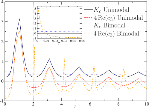
Here, we have used Eq. (56), together with the property that , to obtain the last equality. The sign of given by the last equation gives the nature of the bifurcation as . Note that contrary to similar unstable manifold analysis Crawford:1995 ; Crawford:1995-1 ; Barre:2016 is not diverging as , which validates formally the asymptotic analysis. Equations (57) and (71) suggest that at bifurcation, the effects of changing at a fixed are the same as those from changing at a fixed keeping constant. Interestingly, the sign of predicted by our analysis, which determines the nature of bifurcation, shows oscillations with delay (see Fig. 1) that agree qualitatively with what is observed in many oscillator systems with delayed coupling or control vanderpol:2014 ; delayed_control_2007 ; delay_feedback_2014 .
For a fixed and by varying , one may plot the sign of by computing at criticality and . The result for is shown in Fig. 1 for the case of the Lorentzian frequency distribution, Eq. (10), and also for the case of a sum of two Lorentzians given by
| (72) |
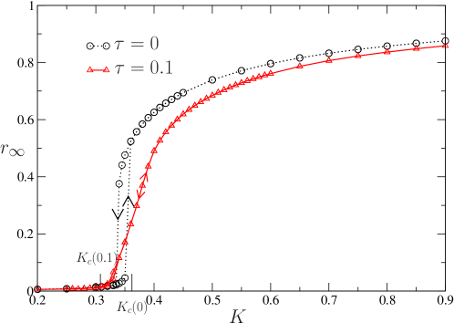
where is the width parameter of each Lorentzian and their center frequencies ( has two separated maxima for ). We show in Fig. 2 that as predicted in Fig. 1 (inset) via the sign of , a very small delay (here ) can suppress the subcritical bifurcation present with a bimodal distribution in the absence of delay and turn it into a supercritical bifurcation. In effect, a subcritical bifurcation means that in the bifurcation regime, a small change in the value of the coupling leads to a large change in the value of the order parameter, that is, an incoherent state becomes with a small change of a synchronized state, and vice versa. On the contrary, a supercritical bifurcation implies that a small change in leads to only a small change in the order parameter, so that tuning of leads to a continuous change of the incoherent into a synchronized state, and vice versa. In the former case of a subcritical bifurcation, it is well known that an adiabatic tuning of , in which is tuned in time at a rate slow enough that the system is very close to the stationary state at every instant, and concomitant monitoring of leads to a hysteresis behavior of as a function of Strogatz-book .
While Fig. 1 represents the results for Lorentzians, it is evident from the nature of the expression (71) that it would be quite a daunting task to make just on the basis of this expression general remarks on the nature of bifurcation for general frequency distributions, and every distribution has to be investigated on a case-by-case basis.
It may be noted that for some special values of delay satisfying for , presence of delay in the cosine term of Eq. (6) has no effect. In this case, if the eigenvalue triggering the instability of the incoherent state is real (for the distribution (72), it corresponds to ), it will be of multiplicity two, so that our derived two-dimensional unstable manifold is still valid. However, if there is a pair of complex eigenvalues (for the distribution (72), it corresponds to ), each one will have a multiplicity of two, and consequently, one should consider instead a four-dimensional unstable manifold, as done for in Ref. Crawford:1994-1 . For , there is a pair of complex eigenvalue of multiplicity one, so that our two-dimensional unstable manifold expansion holds good.
For the Lorentzian distribution, (10), one may check that the normal form obtained from the OA-reduced-dynamics, Eq. (43), and the kinetic equation, Eq. (69), are the same.
For generic , we may decompose as in Eq. (11), with Fourier coefficients , where the ’s are the Fourier coefficients on the unstable manifold. Using Eq. (7), we get . From Eqs. (55) and (59), we get
| (73) |
Notice that expression (73) explicitly satisfies the assumption made by the OA ansatz that as . We cannot prove within the current framework the validity of the OA assumption that . Similarly, Eqs. (68) and (59) give
| (74) |
As in Eq. (67), we may write equations for the Fourier modes with , obtaining
| (75) | |||
| (76) |
where we have used , and the fact that the dominant contribution in Eq. (63) always involves for the term and not . By induction, we deduce for that
| (77) |
and by taking the complex conjugate of the last equation, we obtain the corresponding equation for . These equations clearly show that the unstable manifold has exactly the same form as the OA manifold close to the bifurcation. Note that this feature is valid both in the absence and presence of delay. It is worthwhile to mention that the OA ansatz fails on adding a second harmonic (that is, with the form of interaction ) to Eq. (1), and even the relation (77) obtained with Eq. (76) is also not valid in this case. In fact in this case (without delay) the unstable manifold has been shown to be singular Crawford:1995 ; Crawford:1999 . Nonetheless, the unstable manifold reduction still provided precious informations on the bifurcation. The singularities denote a profound change in the nature of the problem. Studying how Eq. (76) is modified by the addition of a second harmonic or noise could be a starting point for investigations into generalizations of the OA ansatz.
7 Conclusions and perspectives
In this work, we analyzed in detail the consequences of a time delay in the interaction in the case of the Kuramoto model of globally-coupled oscillators with distributed natural frequencies, for generic choice of the frequency distribution . We derived as a function of the delay exact results for the stability boundary between the incoherent and the synchronized state and the nature in which the latter bifurcates from the former at the critical point. Our results are obtained in two independent ways: one, by considering the kinetic equation for the time evolution of the single-oscillator distribution, and two, by considering for the specific choice of a Lorentzian distribution a reduced equation for the order parameter derived from the kinetic equation by invoking the celebrated Ott-Antonsen ansatz. In either case, the incoherent state, in which the oscillators are completely unsynchronized, is a stationary solution for all values of the coupling constant between the oscillators, but which is linearly stable only below a critical value of the coupling. To examine how a stable synchronized state bifurcates from the incoherent state as the coupling crosses the value , we employed an unstable manifold expansion of perturbations about the incoherent state in the vicinity of the bifurcation, which we applied both to the kinetic equation and to the corresponding Ott-Antonsen-reduced dynamics. We found that the nature of the bifurcation is determined by the sign of the coefficient of the cubic term in the equation describing the amplitude dynamics of the unstable modes in the regime of weak linear instability, namely, as . Remarkably, we found that the amplitude equation derived from the kinetic equation has the same form as that obtained from the OA-ansatz-reduced dynamics for the particular case of a Lorentzian , thus confirming the power and general applicability of the OA ansatz. Moreover, quite interestingly, we found that close to the bifurcation, the unstable manifold has the same form as that of the OA manifold. This may have important bearings on their inter-relationship to be unravelled in future. As an explicit physical effect of the presence of delay, we demonstrated with our exact results that for a sum of two Lorentzians as a representative example of a bimodal frequency distribution, while absence of delay leads to a bifurcation of the synchronized from the incoherent state that is subcritical, even a small amount of delay changes completely the nature of the bifurcation and makes it supercritical.
Acknowledgements.
This work was initiated while DM was affiliated to Laboratory J.A. Dieudonné, Université Côte d’Azur, Nice, France and was finalized with DM being affiliated to Los Alamos National Laboratory (LANL). DM gratefully acknowledges the support of the U.S. Department of Energy through the LANL/LDRD Program and the Center for Non Linear Studies, LANL. The paper was written up during the visit of DM and SG to the International Centre for Theoretical Physics – South American Institute for Fundamental Research, São Paulo, Brazil in May 2018 and during SG’s extended stay at the Universidade Federal de São Carlos and the Centro de Pesquisa em Óptica e Fotônica, Sào Carlos, Brazil during June 2018. The authors thank these institutions for warm hospitality and financial support.References
- (1) Y. Kuramoto, Chemical oscillations, waves, and turbulence (Springer-Verlag, Berlin, 1984).
- (2) S. H. Strogatz, From Kuramoto to Crawford: Exploring the onset of synchronization in populations of coupled oscillators, Physica D 143, 1 (2000).
- (3) J. A. Acebrón, L. L. Bonilla, C. J. Pérez Vicente, F. Ritort and R. Spigler, The Kuramoto model: A simple paradigm for synchronization phenomena, Rev. Mod. Phys. 77, 137 (2005).
- (4) S. Gupta, A. Campa and S. Ruffo, Kuramoto model of synchronization: Equilibrium and non-equilibrium aspects, J. Stat. Mech.: Theory Exp. R08001 (2014).
- (5) F. A. Rodrigues, T. K. DM. Peron, P. Ji and J. Kurths, The Kuramoto model in complex networks, Phys. Rep. 610, 1 (2016).
- (6) S. Gherardini, S. Gupta and S. Ruffo, Spontaneous synchronization and nonequilibrium statistical mechanics of coupled phase oscillators, Contemporary Physics 59, 229 (2018).
- (7) S. Gupta, A. Campa and S. Ruffo, Statistical physics of synchronization (Springer-Verlag, Berlin, 2018).
- (8) A. Pikovsky, M. Rosenblum and J. Kurths, Synchronization: a Universal concept in nonlinear sciences (Cambridge University Press, Cambridge, 2001).
- (9) S. H. Strogatz, Sync: the emerging science of spontaneous order (Hyperion, New York, 2003).
- (10) J. Buck, Synchronous rhythmic flashing of fireflies. II., Q. Rev. Biol. 63, 265 (1988).
- (11) C. S. Peskin, Mathematical aspects of heart physiology (Courant Institute of Mathematical Sciences, New York, 1975).
- (12) I. Kiss, Y. Zhai and J. Hudson, Emerging coherence in a population of chemical oscillators, Science 296, 1676 (2002).
- (13) A. A. Temirbayev, Z. Zh. Zhanabaev, S. B. Tarasov, V. I. Ponomarenko and M. Rosenblum, Experiments on oscillator ensembles with global nonlinear coupling, Phys. Rev. E 85, 015204(R) (2012).
- (14) S. P. Benz and C. J. Burroughs, Coherent emission from two‐dimensional Josephson junction arrays, Appl. Phys. Lett. 58, 2162 (1991).
- (15) M. Rohden, A. Sorge, M. Timme and D. Witthaut, Self-Organized synchronization in decentralized power grids, Phys. Rev. Lett. 109, 064101 (2012).
- (16) L. Herrgen, S. Ares, L. G. Morelli, C. Schröter, F. Jülicher and A. C. Oates, Intercellular coupling regulates the period of the segmentation clock, Curr. Biol. 20, 1244 (2010).
- (17) L. Wetzel, D. J. Jörg, A. Pollakis, W. Rave, G. Fettweis and F. Jülicher, Self-organized synchronization of digital phase-locked loops with delayed coupling in theory and experiment. PLoS ONE 12, e0171590 (2017).
- (18) F.-C. Blondeau and G. Chauvet, Stable, oscillatory, and chaotic regimes in the dynamics of small neural networks with delay, Neural Netw. 5, 735 (1992).
- (19) E. Niebur, H. G. Schuster and D. M. Kammen, Collective frequencies and metastability in networks of limit-cycle oscillators with time delay, Phys. Rev. Lett. 67, 2753 (1991).
- (20) M. K. S. Yeung and S. H. Strogatz, Time delay in the Kuramoto Model of coupled oscillators, Phys. Rev. Lett. 82, 648 (1999).
- (21) H. Sakaguchi and Y. Kuramoto, A soluble active rotator model showing phase transitions via mutual entrainment, Prog. Theor. Phys. 76, 576 (1986).
- (22) E. Montbrió, D. Pazó and J. Schmidt, Time delay in the Kuramoto model with bimodal frequency distribution, Phys. Rev. E 74, 056201 (2006).
- (23) E. Ott and T. M. Antonsen, Low dimensional behavior of large systems of globally coupled oscillators, Chaos 18, 037113 (2008).
- (24) E. Ott and T. M. Antonsen, Long time evolution of phase oscillator systems, Chaos 19, 023117 (2009).
- (25) N. J. Balmforth and R. Sassi, A shocking display of synchrony, Physica D, 143, 21 (2000).
- (26) J. A. Carrillo, Y. P. Choi and L. Pareschi, Structure preserving schemes for the continuum Kuramoto model: phase transitions, arXiv preprint arXiv:1803.03886 (2018).
- (27) M. Wolfrum, S. V. Gurevich and O. E. Omel’chenko, Turbulence in the Ott-Antonsen equation for arrays of coupled phase oscillators, Nonlinearity 29, 257 (2016).
- (28) D. Pazó and E. Montbrió, From quasiperiodic partial synchronization to collective chaos in populations of inhibitory neurons with delay, Phys. Rev. Lett. 116, 23 (2016).
- (29) E. A. Martens, C. Bick and M. J. Panaggio, Chimera states in two populations with heterogeneous phase-lag, Chaos 26, 094819 (2016).
- (30) C. R. Laing, Traveling waves in arrays of delay-coupled phase oscillators, Chaos 26, 094802 (2016).
- (31) E. Ott and T. M. AntonsenJr., Frequency and phase synchronization in large groups: Low dimensional description of synchronized clapping, firefly flashing, and cricket chirping, Chaos 27, 051101 (2017).
- (32) D. S. Goldobin, A. V. Pimenova, M. Rosenblum and A. Pikovsky, Competing influence of common noise and desynchronizing coupling on synchronization in the Kuramoto-Sakaguchi ensemble, EPJ ST 226, 1921 (2017).
- (33) X. Zhang, A. Pikovsky and Z. Liu, Dynamics of oscillators globally coupled via two mean fields, Sci. Rep. 7, 2104 (2017).
- (34) J. K. Hale, Linear functional differential equations with constant coefficients, Contributions to Differential Equations 2, 291 (1963).
- (35) J. K. Hale and S. M. V. Lunel, Introduction to functional differential equations (Springer-Verlag, New York, 1993).
- (36) J. D. Crawford, Amplitude expansions for instabilities in populations of globally-coupled oscillators, J. Stat. Phys. 74, 1047 (1994).
- (37) J. D. Crawford, Universal trapping scaling on the unstable manifold for a collisionless electrostatic mode, Phys. Rev. Lett. 73, 656 (1994).
- (38) J. D. Crawford, Scaling and singularities in the entrainment of globally coupled oscillators, Phys. Rev. Lett. 74, 4341 (1995).
- (39) J. D. Crawford, Amplitude equations for electrostatic waves: universal singular behavior in the limit of weak instability, Physics of Plasmas 2, 97 (1995).
- (40) J. D. Crawford and K. T. R. Davies, Synchronization of globally coupled phase oscillators: singularities and scaling for general couplings, Physica D 125, 1 (1999).
- (41) J. Barré and D. Métivier, Bifurcations and singularities for coupled oscillators with inertia and frustration, Phys. Rev. Lett. 117, 214102 (2016).
- (42) E. A. Martens, E. Barreto, S. H. Strogatz, E. Ott, P. So and T. M. Antonsen Exact results for the Kuramoto model with a bimodal frequency distribution, Phys. Rev. E 79, 026204 (2009).
- (43) T. D. Frank, Kramers-Moyal expansion for stochastic differential equations with single and multiple delays: Applications to financial physics and neurophysics, Phys. Lett. A 360, 552 (2007).
- (44) Dietert H and Fernandez B. The mathematics of asymptotic stability in the Kuramoto model, Proceedings of the Royal Society A. (2018) 12;474(2220):20180467.
- (45) J. Murdock, Normal forms and unfoldings for local dynamical systems (Springer-Verlag, New York, 2006).
- (46) S. Guo and J. Wu, Bifurcation theory of functional differential equations (Springer-Verlag, New York, 2013).
- (47) B. Niu and Y. Guo, Bifurcation analysis on the globally coupled Kuramoto oscillators with distributed time delays, Physica D 266, 23 (2014).
- (48) H. Chiba, A proof of the Kuramoto conjecture for a bifurcation structure of the infinite-dimensional Kuramoto model, Ergodic Theory and Dynamical Systems 35, 762 (2013).
- (49) H. Dietert, Stability and bifurcation for the Kuramoto model, Journal de Mathématiques Pures et Appliquées 105, 451 (2016).
- (50) S. H. Strogatz, Nonlinear Dynamics and Chaos: with Applications to Physics, Biology, Chemistry, and Engineering (Westview Press, Boulder, 2014).
- (51) J. D. Crawford and P. D. Hislop, Application of the method of spectral deformation to the Vlasov-poisson system, Annals of Physics 189, 265 (1989).
- (52) S. H. Strogatz and R. E. Mirollo, Stability of incoherence in a population of coupled oscillators, J. Stat. Phys. 63, 613 (1991).
- (53) S. H. Strogatz, R. E. Mirollo and P. C. Matthews, Coupled nonlinear oscillators below the synchronization threshold: relaxation by generalized Landau damping, Phys. Rev. Lett. 68, 2730 (1992).
- (54) A. Y. T. Leung, H. X. Yang and P. Zhu, Periodic bifurcation of Duffing-van der Pol oscillators having fractional derivatives and time delay, Communications in Nonlinear Science and Numerical Simulation 19, 1142 (2014).
- (55) X. Xu, H. Y. Hu and H. L. Wang, Stability, bifurcation and chaos of a delayed oscillator with negative damping and delayed feedback control, Nonlinear Dyn 49, 117 (2007).
- (56) Chol-Ung Choe, Ryong-Son Kim, Hyok Jang, P. Hövel and E. Schöll, Delayed-feedback control: arbitrary and distributed delay-time and noninvasive control of synchrony in networks with heterogeneous delays, Int. J. Dynam. Control 2, (2014).