Digitization of Scalar Fields for Quantum Computing

Abstract

Qubit, operator and gate resources required for the digitization of lattice $\lambda\phi^{4}$ scalar field theories onto quantum computers are considered, building upon the foundational work by Jordan, Lee and Preskill, with a focus towards noisy intermediate-scale quantum (NISQ) devices. The Nyquist-Shannon sampling theorem, introduced in this context by Macridin, Spentzouris, Amundson and Harnik building on the work of Somma, provides a guide with which to evaluate the efficacy of two field-space bases, the eigenstates of the field operator, as used by Jordan, Lee and Preskill, and eigenstates of a harmonic oscillator, to describe $0+1$- and $d+1$-dimensional scalar field theory. We show how techniques associated with improved actions, which are heavily utilized in Lattice QCD calculations to systematically reduce lattice-spacing artifacts, can be used to reduce the impact of the field digitization in $\lambda\phi^{4}$, but are found to be inferior to a complete digitization-improvement of the Hamiltonian using a Quantum Fourier Transform. When the Nyquist-Shannon sampling theorem is satisfied, digitization errors scale as $|\log|\log|\epsilon_{\rm dig}|||\sim n_{Q}$ (number of qubits describing the field at a given spatial site) for the low-lying states, leaving the familiar power-law lattice-spacing and finite-volume effects that scale as $|\log|\epsilon_{\rm latt}||\sim N_{Q}$ (total number of qubits in the simulation). For localized(delocalized) field-space wavefunctions, it is found that $n_{Q}\sim 4(7)$ qubits per spatial lattice site are sufficient to reduce theoretical digitization errors below error contributions associated with approximation of the time-evolution operator and noisy implementation on near-term quantum devices.

I Introduction

While offering the potential to greatly refine calculations that can be performed through classical computation, Quantum Computing (QC) also holds the potential to enable calculations of quantities in quantum field theories and other quantum many-body systems that are not possible with classical techniques Lloyd (1996); Ortiz et al. (2001); Somma et al. (2002); Byrnes and Yamamoto (2006); Ovrum and Hjorth-Jensen (2007); Jordan et al. (2011, 2012, 2014, 2018); Zohar et al. (2013, 2012); Banerjee et al. (2012, 2013); Wiese (2013); Marcos et al. (2014); Wiese (2014); Zohar et al. (2017); Bermudez et al. (2017); Banuls et al. (2017); Kaplan and Stryker (2018). In particular, real-time dynamics, such as the fragmentation of quarks into hadrons at particle accelerators, the dynamics of non-equilibrium systems, and the nature of finite-density systems for which sampling with classical computation is limited by sign problems, are key areas for which a quantum advantage is anticipated to be achieved. Quantum devices with a range of underlying qubit architectures without error correction are now becoming available for domain scientists to seek inroads into these problems and other important scientific applications, and to envisage attributes of quantum devices necessary to outperform classical computations of scientific significance. The performance of present day quantum devices is limited by a number of basic attributes, including coherence times and the number of gates (specifically entangling gates) that can be applied prior to decoherence, the accuracy and precision of applied gates, the number and interconnectivity of qubits, and the lack of error correction. While significant efforts are in progress to reduce or eliminate these deficiencies, and remarkable progress is being made, these limitations are expected to persist in near-term quantum devices. This has led John Preskill to name the present and upcoming time period the “NISQ era” (Noisy Intermediate-Scale Quantum era) Preskill (2018). While formidable in its destruction of pure quantum states, quantum noise has been recently suppressed sufficiently for a number of small quantum simulations of physical systems Martinez et al. (2016); O’Malley et al. (2016); Kandala et al. (2017); Dumitrescu et al. (2018); Klco et al. (2018); Hempel et al. (2018), encouraging the expectation of meaningful scientific applications of NISQ-era devices.

Scalar field theories are ubiquitous in physics, from describing densities in condensed matter systems, to fundamental fields in the electroweak sector from which the Higgs Boson emerges after spontaneous symmetry breaking. The quantum theory describing the dynamics of a self-interacting, real scalar field represents, perhaps, the simplest quantum field theory (QFT) that can be explored through direct digitization of the field with a quantum computer. Such studies are anticipated to provide important insights into how quantum devices can be used to simulate gauge field theories, such as quantum electrodynamics (QED) and quantum chromodynamics (QCD) that describe the interactions in electronic systems and between quarks and gluons responsible for the nuclear forces and the structure and dynamics of strongly interacting matter. It is exciting to observe the advances that are being made in developing Jordan et al. (2011, 2012, 2014, 2018); Wiese (2013, 2014); García-Álvarez et al. (2015); Bazavov et al. (2015); Zohar et al. (2016); Pichler et al. (2016); Bermudez et al. (2017); Banuls et al. (2017); Moosavian and Jordan (2017); Gonzalez-Cuadra et al. (2017); Macridin et al. (2018a); Klco et al. (2018); Zhang et al. (2018); Macridin et al. (2018b); Kaplan and Stryker (2018); Bender et al. (2018); Zohar and Cirac (2018); Zohar (2018); Jefferson and Myers (2017); Alsup et al. (2016); Yeter-Aydeniz and Siopsis (2018); Marshall et al. (2015); Bradler et al. (2016) and implementing Zohar et al. (2013, 2012); Banerjee et al. (2013, 2012); Marcos et al. (2014); Marshall et al. (2015); Zohar et al. (2017); Martinez et al. (2016); Muschik et al. (2017); Klco et al. (2018) algorithms for both Abelian and non-Abelian gauge theories and scalar field theories that may be useful for QFT calculations with quantum computers.

It is not expected that NISQ-era devices will surpass the computational capabilities of classical devices for the evolution of scalar fields discussed in this paper. While an advantage may be found in a contrived endeavour for increased precision in the ground state energy of a non-local spatial wavefunction (see section IV.3.1), the more-likely regimes of quantum advantage in simulation are those highlighted at the beginning of this introduction. Creating a computational framework making these systems accessible, taking advantage of superpositions and interference while remaining robust to quantum noise, is arduous and has become the focus of many current avenues of research; porting the knowledge and understanding of high-performance classical computation will be vital but insufficient to achieve this goal. As is the case in classical computing, performance and scaling of quantum devices for scientific application cannot be completely understood before computations are implemented at scale on hardware. While quantum calculations at scale are unreasonable today and the currently-available hardware is likely far from future fault-tolerant devices, this document examines scalar quantum field theory calculations on near-term quantum devices in preparation for a future in which substantial quantum resources allow exploration of classically-unattainable states of matter.

In a series of foundational papers, Jordan, Lee and Preskill (JLP) formulated and analyzed scalar field theories for quantum computers Jordan et al. (2011, 2012, 2014, 2018) and estimated the resource-requirement scaling of calculations of static properties and of elastic and inelastic particle scattering processes determined through direct time evolution. A real scalar field, $\phi({\bf x})$, is discretized on a spatial lattice using techniques that are standard in lattice QCD (LQCD) calculations using classical computers. The spacing between lattice sites along a cartesian axis is denoted by $a$ and the extent of each spatial direction is denoted by $L$, and $\phi({\bf x})$ is subject to, for example, periodic boundary conditions (PBCs) or twisted boundary conditions (e.g. Refs. Lin et al. (2001); Sachrajda and Villadoro (2005); Bedaque (2004); Briceno et al. (2014)) in each direction. However, in NISQ-era quantum computations, $\phi({\bf x})$ can only assume values from a modest-sized set of possibilities, with extreme values of $|\phi({\bf x})|\leq\phi_{\rm max}$ and a digitization $\delta_{\phi({\bf x})}$. Therefore, the computational layout of these JLP simulations is that a number of qubits, $n_{Q}$, describe the value of $\phi({\bf x})$ at each position ${\bf x}$, with a total number of qubits of $N_{Q}=n_{Q}\left(L/a\right)^{d}$ for spatial dimension, $d$. This system is evolved under the action of the time-evolution operator, $\hat{U}(t)=e^{-i\hat{H}t}$ where $\hat{H}$ is the Hamiltonian operator, to evolve isolated wave packets forward in time to determine scattering amplitudes.

In nice work by Macridin, Spentzouris, Amundson and Harnik (MSAH) Macridin et al. (2018a, b), focused on phonon-electron interactions and building upon work by Somma Somma (2016), it was emphasized that the Nyquist-Shannon (NS) sampling theorem should be considered in the architecture of a quantum computer, the mapping of $\phi({\bf x})$ and the implementation of the Hamiltonian to achieve the desired accuracies in quantum simulations. The localization of the $\phi({\bf x})$ wavefunction in $\phi$-space and its curvature determine the extent and interval of sampling in $\phi$-space, i.e. $\phi_{\rm max}$ and $\delta_{\phi({\bf x})}$ (which dictate $n_{Q}$), required to reproduce the $\phi$-space wavefunction with exponential precision, scaling as $|\log|\log|\epsilon_{\rm dig}|||\sim n_{Q}$, where $\epsilon_{\rm dig}$ is the error introduced through digitization, thereby removing inaccuracies due to field digitization. These studies of the NS sampling theorem determined the minimum number of qubits per phonon field required to accurately describe harmonic oscillator (HO) wavefunctions up to a given excitation level of the phonon field Somma (2016); Macridin et al. (2018a, b). The digitization errors make contributions that are parametrically smaller than spatial lattice-spacing artifacts and spatial finite-volume effects, which typically scale as $|\log|\epsilon_{\rm latt}||\sim N_{Q}$, where $\epsilon_{\rm latt}$ is the error introduced by the non-zero spatial lattice spacing.

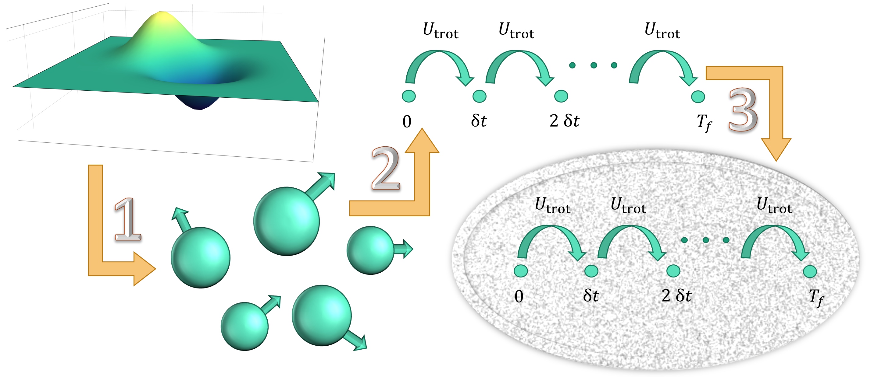
Figure 1: Identifying three distinct sources of error in quantum simulations of scalar field theory: (1) the error of digitizing and latticizing the continuous field onto qubit degrees of freedom; (2) the error of simulation due to the use of approximations to the exact digitized propagator; (3) the error due to noise in the quantum device’s implementation of the approximate digitized propagator. The first two sources of error are independent of the quantum hardware. The first is the main focus of this paper.

The use of $\epsilon$ in this paper indicates the precision to which the ground state energy of the continuous scalar field can be reproduced by a Hamiltonian digitized with qubit degrees of freedom (step (1) of Fig. 1). This is a theoretical source of systematic error accompanying the formulation of the Hamiltonian before it is implemented on hardware or employed in a simulation algorithm. Most importantly, this is not the $\epsilon$ commonly used in the quantum simulation literature to express the precision with which properties of a given Hamiltonian can be extracted on quantum hardware (steps (2,3) of Fig. 1). Thus, $\epsilon$ here characterizes the physics of field-digitization necessary to map the system onto a qubit Hamiltonian, and does not include precision reductions entering from the Hamiltonian simulation (e.g., Trotterization) or phase estimation that may be implemented to extract features of this system on quantum hardware. Examples of progress in bounding these latter sources of error can be found in Refs. Wecker et al. (2014); Reiher et al. (2017); Poulin et al. (2015); Babbush et al. (2015); Hao Low and Chuang (2016). The distinction between these three sources of error are depicted in Fig. 1. The scalar field begins in a continuous representation in a formally-infinite-dimensional Hilbert space. With the reduction in step (1), this infinite dimensional Hilbert space is truncated, digitized, and formulated on qubit degrees of freedom. Step (2) designs a quantum simulation algorithm to approximate the time evolution of the quantum state e.g., Trotterization, which introduces errors scaling polynomially in the temporal digitization step size $\delta t$. Step (3) implements this approximate time evolution on quantum hardware susceptible to noise and (likely) without quantum error correction in the NISQ-era.

The digitization errors represented in step (1) of Fig. 1 are the only errors considered in the main text of this paper. The results presented in this work establish the precision of low-energy calculations that could be obtained on an ideal quantum device with exact implementation of the time evolution operator based upon formal considerations of digitizations and discretizations that must be performed when formulating the field theories onto quantum devices with a modest number of qubits. These are presented in order to determine the best-case scenarios for modest-sized devices of the near term, and intentionally neglect the errors of steps (2,3) necessary to accurately reflect the precision attainable with realistic NISQ-era devices. Simulations of the effects of first-order Trotterization (2) and simple unitary gate noise (3) can be found in Appendix H. Together, Appendix H and the main text indicate that digitization errors (1) may be controlled to high precision with a number of qubits reasonable for the NISQ era, leaving the steps (2,3) to dominate the current scalar simulation error budget.

In this work, we consider implications of the digitization of scalar fields when mapped to qubit degrees of freedom, with a focus on the associated limits in accuracy of calculations on NISQ-era scale devices. In particular, we examine digitizing 0+1 and 1+1 dimensional $\lambda\phi^{4}$ scalar field theory describing a single real scalar field, including estimating qubit requirements, estimating the number of operators and number of gates required for such simulations, and extrapolating these estimates to $d$+1-dimensional simulations . As the sign of the mass-squared term in the Hamiltonian determines whether the ground state of these theories are localized around $\phi=0$ or are delocalized around two minima of the potential, estimates are provided for both situations. Making a connection with classical calculations of lattice QFTs, we discuss Hamiltonian improvement that can be included to parametrically reduce the impact of the field digitization by powers of $\delta_{\phi({\bf x})}^{2}$. However, as used in Refs. Jordan et al. (2011, 2012, 2014, 2018) and emphasized in Refs. Somma (2016); Macridin et al. (2018a, b), the use of the Quantum Fourier Transform (QuFoTr) on the $n_{Q}$ qubits at each spatial site to evaluate the action of the conjugate-momentum term in the Hamiltonian, and the freedom it provides in applying phases in field conjugate-momentum space, provides the opportunity to arbitrarily improve the digitized Hamiltonian, removing all polynomials in $\delta_{\phi({\bf x})}$ and rendering digitization effects to be exponentially small (once the conditions imposed by the NS sampling theorem are satisfied). Analogous implementations have been utilized previously in Monte-Carlo calculations of non-relativistic systems Bulgac et al. (2008); Endres et al. (2013). We present the complete operator structure required to implement simulations with $n_{Q}=3,4,5$ qubits per spatial site, along with associated quantum circuits for $n_{Q}=3$. As different bases in $\phi$-space can be used to span the Hilbert space at each point in space, we examine the JLP implementation using the eigenstates of the $\phi$-operator and a basis defined by the eigenstates of a harmonic oscillator (HO), that is distinct from the frameworks developed in Refs. Somma (2016); Macridin et al. (2018b, a). From our analysis, we conclude that the properties and dynamics of interacting scalar field theories may be simulated with only a modest number of qubits per site required to render digitization artifacts negligible compared to other expected systematic errors in the NISQ-era.

II Lattice Scalar Field Theory with Qubits

The continuum Lagrange density describing the dynamics of a scalar field with self interactions, retaining only renormalizable terms in 3+1 dimensions, is

$${\cal L} = {1\over 2}(\partial_{\mu}\phi)^{2}-{1\over 2}m^{2}\phi^{2}-{\lambda\over 4!}\phi^{4}\ \ \ ,$$ (1)

with a Hamiltonian density of

$${\cal H} = {1\over 2}\Pi^{2}+{1\over 2}({\bm{\nabla}}\phi)^{2}+{1\over 2}m^{2}\phi^{2}+{\lambda\over 4!}\phi^{4}\ \ \ .$$ (2)

The conjugate momentum operator, $\Pi({\bf x})$ has the standard equal-time commutation relation with the field operator, $\left[\ \phi({\bf x}),\Pi({\bf y})\ \right]=i\delta^{3}({\bf x}-{\bf y})$. Numerical evaluation of observables resulting from this Hamiltonian density can be accomplished by discretizing space with a cubic grid with a distance between adjacent lattice sites on the Cartesian axes of $a$ (the lattice spacing) and extent $L$ in each direction, as previously defined. The number of sites in each spatial direction is $L/a$. The discretized Hamiltonian on a $d$-dimensional spatial lattice is

$$H = a^{d}\ \sum_{\bf x}\ {1\over 2}\Pi^{2}-{1\over 2}\phi{\bm{\nabla}}^{2}_{a}\phi+{1\over 2}m_{0}^{2}\phi^{2}+{\lambda_{0}\over 4!}\phi^{4}\ \ \ ,$$ (3)

where the discretized Laplacian operator is defined as ${\bm{\nabla}}^{2}_{a}\phi({\bf x})=\sum\limits_{j=1}^{d}\left(\phi({\bf x}+a\hat{\mu}_{j})+\phi({\bf x}-a\hat{\mu}_{j})-2\phi({\bf x})\right)/a^{2}$ where $\hat{\mu}_{j}$ is the unit vector in the $j^{\rm th}$ direction. The quantities $m_{0}$ and $\lambda_{0}$ are bare parameters that are tuned to recover, for example, correct values of the $\phi$ mass, $M_{\phi}$, and the $4\phi$ scattering amplitude. The conjugate momentum is required to satisfy

$$\left[\ \phi({\bf x}),\Pi({\bf y})\ \right] = {i\over a^{d}}\delta^{d}_{{\bf x},{\bf y}}\ \hat{I}\ \ \ ,$$ (4)

where $\hat{I}$ is the identity operator in field space. Redefining the fields, Hamiltonian and mass as $\hat{\phi}=a^{(d-1)/2}\phi$, $\hat{\Pi}=a^{(d+1)/2}\Pi$, $\hat{H}=aH$, $\hat{m}_{0}=am_{0}$, $\hat{\lambda}_{0}=a^{3-d}\lambda_{0}$, Eq. (3) can be written in terms of dimensionless quantities,

$$\hat{H} = \sum_{\bf x}\ {1\over 2}\hat{\Pi}^{2}-{1\over 2}\hat{\phi}\hat{\bm{\nabla}}^{2}_{a}\hat{\phi}+{1\over 2}\hat{m}_{0}^{2}\hat{\phi}^{2}+{\hat{\lambda}_{0}\over 4!}\hat{\phi}^{4}\ \ \ ,$$ (5)

with an equal-time commutator of

$$\left[\ \hat{\phi}({\bf x}),\hat{\Pi}({\bf y})\ \right] = i\delta^{d}_{{\bf x},{\bf y}}\ \hat{I}\ \ \ .$$ (6)

The eigenstates of the momentum operator, $|{\bf k}\rangle$, satisfy $\hat{\cal K}|{\bf k}\rangle={\bf k}|{\bf k}\rangle$ where ${\bf k}$ is quantized by the boundary conditions, and, for example, takes the values ${\bf k}={\bf n}{2\pi\over L}$ for PBCs, where the integer-triplets ${\bf n}$ are constrained to lie within the first Brillouin zone $|n_{x,y,z}|<{L\over 2a}$. The finite-difference operator that is used to define the latticized $\hat{\bf K}=\hat{\bm{\nabla}}^{2}_{a}\hat{\phi}$ has eigenvalues such that $\hat{\bf K}|{\bf k}\rangle=\hat{\bf k}|{\bf k}\rangle$ with $\hat{k}_{j}={2\over a}\sin\left({k_{j}a\over 2}\right)$.

The construction of the latticized Hamiltonian in Eq. (5) is such that the long-distance, or low-energy, quantities (compared to $\pi/a$) will be faithfully reproduced in numerical evaluations up to corrections that are polynomial in the lattice spacing, $\sim(aE)^{n}$, or exponential in the volume, $\sim e^{nM_{\phi}L}$ (for spatially localized states). Therefore, such lattice frameworks should be considered as low-energy effective field theories (EFTs), with an ultra-violet (UV) cut-off set by the inverse lattice spacing. Considerable effort by the LQCD community has been put in to construct improved actions in which additional terms are added to the Lagrange density that are parametrically suppressed by powers of the lattice spacing and consistent with the underlying (hyper-)cubic symmetry of the spacetime lattice. The additional terms in the QCD action are termed the Symanzik action Symanzik (1983a, b). Coefficients of the operators in the Symanzik action depend upon the lattice spacing and the discretized action, and are determined both by tree-level matching and nonperturbatively through tuning for higher precision. As an example, the Wilson discretization of the light-quark field in LQCD calculations leads to spatial finite-difference discretization errors that scale linearly with the lattice spacing, ${\cal O}(a)$. By adding one dimension-5 operator to the lattice action, the Sheikholeslami-Wohlert term Sheikholeslami and Wohlert (1985), and tuning its coefficient, this improved action produces low-energy and long-distance observables that have errors at ${\cal O}(a^{2})$. In principle, an arbitrary number of operators in the Symanzik action can be included in numerical computations to improve the action to high orders. However, the requirements for such calculations that include, for instance, four-quark operators, make this impractical. We will apply similar considerations when proposing improvements for the digitization of the scalar field onto quantum degrees of freedom.

III Implications of the Nyquist-Shannon Sampling Theorem

The work of MSAH Macridin et al. (2018a, b) stressed the importance of the NS Sampling Theorem, implicit in the work of Somma Somma (2016), which is central to signal processing, communications and data compression, to quantum computations. It is worth reminding the reader of its main elements and implications. While the results of this theorem are used implicitly in the formulation and analysis of LQCD calculations, connections between the two are typically not dwelt upon.

Consider the reconstruction of a real function, $C(x)$, that has support only between $x=0$ and $x=x_{\rm max}$ in position space and between $k=-k_{\rm max}$ and $k=+k_{\rm max}$ in momentum space, from discrete sampling. If $C(x)$ is sampled over the interval $x\in\left[0,L\right]$ with $L>x_{\rm max}$ and at intervals of $\delta x<{\pi\over k_{\rm max}}$ then the NS Sampling Theorem ensures that $C(x)$ can be reconstructed up to corrections that are exponentially small. The Poisson resummation formula is at the heart of this result, which is also used extensively in deriving, for example, finite-volume effects in LQCD calculations. The implications of this theorem are clear. As long as the function is sampled in both position-space and momentum-space over the entire region where the function has support, then it can be reconstructed with only exponentially small errors introduced by the discretization. In quantum simulations of field theories, and in particular the computation of the low-lying eigenstates and eigenvalues, this imposes constraints for both the spatial discretization and the digitization of the field at any given spatial site. From the viewpoint of lattice calculations, this dictates that the lattice spacing must be small enough to include all spatial-momentum states that contribute (to the level of precision to which the calculation is being performed), and the volume large enough to contain the eigenstates of interest, in order for deviations between the calculated eigenstates and eigenvalues and the true eigenstates and eigenvalues to be exponentially small. For LQCD calculations, this underpins Lüscher’s finite-volume analysis of QCD observables Lüscher (1986a, b, 1991), which is used extensively to both quantify uncertainties and to extract S-matrix elements.

The NS theorem does not specify how to “cover” the region of support in position-space and momentum-space, i.e. what basis should be used to span the spaces, and some bases will be better than others for any given function. For smooth functions that fall exponentially (or as a Gaussian) at large distances, the plane-wave basis is efficient, defined over the spatial interval where the function has support and with a discretization that encompasses its highest frequency component. For a more localized function, such as those that fall as a Gaussian at large distance, eigenstates of the HO that are approximately tuned to the function can also be efficient.

For quantum computations of a field theory using a given set of basis functions to define the spatial discretization and the field digitization, including plane waves or eigenstates of the HO, this theorem dictates the number of qubits required to achieve a desired accuracy. The number of qubits and the number and complexity of operators required to execute the computation are basis dependent. Identifying the optimal basis with which to perform the quantum computation requires examining both the number of qubits and the number of gates required to perform the computation with the desired precision.

It is worth commenting that the NS sampling bounds are likely satisfied in LQCD calculations of localized quantities, such as hadron masses and nuclear bound states. Therefore, the eigenvalues and eigenstates obtained in such calculations would be exponentially close to the values associated with the lattice Hamiltonian if infinite statistics were accumulated in the stochastic sampling of the quantum fields. The power-law deviations that scale as $\sim(aE)^{n}$ result from deviations in the lattice Hamiltonian from the continuum Hamiltonian and are not due to under-sampling in the NS sense. We are unaware of the NS theorem being implemented in classical quantum Monte-Carlo calculations, and consider the possibility worthwhile to explore.

IV 0+1 Dimensional Scalar Field Theory

In order to demonstrate some important features of the construction presented in the previous section, we examine a 0+1 dimensional non-interacting scalar field theory, which is simply a HO. After a further field and Hamiltonian redefinition, $\hat{\phi}={1\over\sqrt{\hat{m}_{0}}}\bar{\phi}$, $\hat{\Pi}=\sqrt{\hat{m}_{0}}\bar{\Pi}$, $\hat{H}=\hat{m}_{0}\bar{H}$, the HO is described by the Hamiltonian,

$$\bar{H} = {1\over 2}\bar{\Pi}^{2}+{1\over 2}\bar{\phi}^{2}\ \ \ ,$$ (7)

with a commutation relation $\left[\ \bar{\phi},\bar{\Pi}\ \right]=i\hat{I}$. It is the digitization of this system that was studied by Somma Somma (2016) and by MSAH Macridin et al. (2018a, b) with the identification $\bar{\phi}\rightarrow X$, $\bar{\Pi}\rightarrow P$ and $\bar{H}\rightarrow H_{h}$. Without field digitization, $\delta_{\bar{\phi}}=0$, this is simply the Hamiltonian describing a HO without self-interactions, with energy eigenstates $|\psi_{n}\rangle$ and energy eigenvalues $E_{n}=n+{1\over 2}$. The conjugate momentum operator can be identified with a derivative in field space, $\bar{\Pi}=-i{d\over d\bar{\phi}}$, to satisfy the equal-time commutation relation.

IV.1 Jordan-Lee-Preskill Basis

When the field is digitized, $\bar{\phi}\rightarrow\tilde{\phi}$ (using the notation of MSAH), and sampled at regular intervals $\delta_{\tilde{\phi}}\neq 0$, the conjugate momentum operator can be replaced by a finite difference operator in field space, in analogy with lattice field theory spatial discretization. It has a matrix representation in $\tilde{\phi}$-space of

$$\langle\tilde{\phi}^{\prime}|\ \tilde{\Pi}^{2}\ |\tilde{\phi}\rangle = {1\over\delta_{\bar{\phi}}^{2}}\ \left(\begin{array}[]{cccccc}2&-1&0&0&\cdots&-1\\ -1&2&-1&0&0&\cdots\\ \vdots&\vdots&\vdots&\vdots&\vdots&\vdots\\ 0&0&\cdots&-1&2&-1\\ -1&0&0&\cdots&-1&2\\ \end{array}\right)\ \ \ ,$$ (13)

and acts in the space defined by field values $-\bar{\phi}_{\rm max},-\bar{\phi}_{\rm max}+\delta_{\tilde{\phi}},\cdots,-\frac{\delta_{\tilde{\phi}}}{2},\frac{\delta_{\tilde{\phi}}}{2},\cdots,\bar{\phi}_{\rm max}-\delta_{\tilde{\phi}},\bar{\phi}_{\rm max}$. For a space spanned by $n_{s}=2^{n_{Q}}$ basis states in field space, the field takes values

$$\bar{\phi} = -\bar{\phi}_{\rm max}\ +\ \delta_{\tilde{\phi}}\ \beta_{\phi}\ \ ,\ \ \delta_{\tilde{\phi}}\ =\ {2\bar{\phi}_{\rm max}\ \over n_{s}-1}\ \ \ ,$$ (14)

where $\beta_{\phi}\ =\ 0,1,...,n_{s}-1$. Note that this formulation allows the field operator to be decomposed as $\phi=\frac{\bar{\phi}_{\rm max}}{n_{s}-1}\sum\limits_{j=0}^{n_{Q}-1}2^{j}\sigma^{z}_{j}$ (with qubits labeled right to left in tensor product spaces) and thus requires only single-qubit Pauli-Z operators for its implementation. As is familiar from classical lattice simulations, the momentum modes of this system satisfying PBCs are,

$$k_{\tilde{\phi}} = -k_{\tilde{\phi}}^{\rm max}+\beta_{k}\ \delta k_{\tilde{\phi}}\ \ ,\ \ k_{\tilde{\phi}}^{\rm max}\ =\ {\pi\over\delta_{\tilde{\phi}}}\ \ ,\ \ \delta k_{\tilde{\phi}}\ =\ {2\pi\over\delta_{\tilde{\phi}}n_{s}}\ \ \ ,$$ (15)

with $\beta_{k}\ =\ 1,2,...,n_{s}$. It is interesting to note that this conjugate momentum-space basis may not be optimal in terms of the number of gates in a quantum circuit required to apply the Hamiltonian to any given state. Satisfying the NS theorem does not require any particular momentum components to be present in the conjugate momentum-space basis set and, as such, there is freedom to shift each momentum state by the same constant momentum. It is convenient to shift each basis state in conjugate momentum space by $\Delta k_{\tilde{\phi}}=-\delta k_{\tilde{\phi}}/2$, so that

$$k_{\tilde{\phi}}^{\Delta} = -k_{\tilde{\phi}}^{\rm max}+\left(\beta_{k}-{1\over 2}\right)\ \delta k_{\tilde{\phi}}\ \ \ ,$$ (16)

which is equivalent to imposing twisted boundary conditions in field space Lin et al. (2001); Sachrajda and Villadoro (2005); Bedaque (2004); Briceno et al. (2014), resulting in $+1$’s in the off-diagonal corners of Eq. (13) and momentum states that are symmetrically distributed within the edges of the first Brillouin zone between values of $\pm\frac{\pi}{\delta_{\tilde{\phi}}}\frac{n_{s}-1}{n_{s}}$. For any choice of basis states spanning conjugate momentum space, the finite-difference operator has matrix elements

$$\langle k_{\tilde{\phi}}^{\prime}|\ \tilde{\Pi}^{2}\ |k_{\tilde{\phi}}\rangle = \hat{k}_{\tilde{\phi}}^{2}\ \delta_{k_{\tilde{\phi}},k_{\tilde{\phi}}^{\prime}}\ \ \ ,\ \ \ \ \hat{k}_{\tilde{\phi}}^{2}\ =\ {4\over\delta_{\tilde{\phi}}^{2}}\ \sin^{2}\left({k_{\tilde{\phi}}\ \delta_{\tilde{\phi}}\over 2}\right)\ \ \ .$$ (17)

The Hamiltonian resulting from this field digitization is denoted by $\bar{H}\rightarrow\tilde{H}$. The precision expected from computations on an ideal quantum computer for a range of values of $\bar{\phi}_{\rm max}$ is shown in Fig. 2. Encouragingly, this calculation indicates that a $\bar{\phi}_{\rm max}$ of 4.7 for a 4-qubit representation of the scalar field can achieve a precision of better than $10^{-3}$% on the energies of the lowest 5 eigenstates of the HO with an ideal quantum simulation.

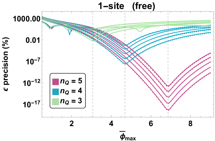
Figure 2: The precision of the energies of the lowest five states of the HO in Eq. (7) expected from calculations on an ideal quantum computer with JLP digitizations over a range of values of $\bar{\phi}_{\rm max}$ for a system digitized on $n_{Q}=3$, $n_{Q}=4$ and $n_{Q}=5$ qubits (minimized at $\bar{\phi}_{\rm max}=$3.1, 4.7, and 6.9, respectively) . The vertical gray-dashed lines correspond to saturation of the NS sampling bound.

For explicit examples of this field digitization implementation with three, four, and five qubits per site, see Appendix A.

With any finite computing device, classical or quantum, only a finite representation of a continuous quantity is possible. In the JLP formulation, $|\phi|$ is bounded by $\phi_{\rm max}$ and sampled at intervals dictated by the number of qubits per site. Focusing on the $\phi_{\rm max}$ truncation of the scalar field and allowing an infinite momentum-space coverage, formal quantum field theory studies Meurice (2002); Kessler et al. (2004) have shown that the asymptotic perturbative series becomes convergent. For a sufficiently large $\phi_{\rm max}$, results for low-lying quantities are exponentially close to those obtained with unbounded values of the field.

In a quantum simulation of this HO, the JLP framework using the eigenstates of $\tilde{\phi}$ and its conjugate momentum can be used, as discussed above. By tuning $\bar{\phi}_{\rm max}$ to be larger than the spatial support of the $n^{\rm th}$ state of the HO at some level of precision, the NS sampling bound will be satisfied for these levels as long as the largest value of $|k_{\tilde{\phi}}|$ in Eq. (15) is greater than the region of support in conjugate momentum-space of the $n^{\rm th}$ state. The action of the Hamiltonian on this set of qubits is most easily accomplished in two parts, as prescribed by JLP. First, the $\tilde{\phi}^{2}$ operator, represented by a diagonal matrix in this basis, is directly evaluated. Second, a QuFoTr is performed to render the matrix representation of $\tilde{\Pi}^{2}$ diagonal and thus easily evaluated. The ability to move back and forth between representations in which $\tilde{\phi}$ or $\tilde{\Pi}$ is diagonal is typically not practical in classical field theory computations and permits more freedom in choosing the operators that can be applied in either representation. Using the $\tilde{\Pi}$ operator in momentum space that is conjugate to the finite-difference operator, Eq. (17), yields exponentially-converged eigenvalues and eigenvectors for the lowest $n$ states (by the NS sampling theorem). However, these quantities differ from the corresponding HO quantities by even powers of $\delta_{\tilde{\phi}}$ because of the difference between $\hat{k}_{\tilde{\phi}}^{2}$ and $k_{\tilde{\phi}}^{2}$ in Eq. (17), as shown in Fig. 3. However, if instead, the $k_{\tilde{\phi}}^{2}$ eigenvalues in $\tilde{\Pi}^{2}$ are used in the quantum computation, corresponding to using $\bar{\Pi}^{2}$ and not $\tilde{\Pi}^{2}$, the eigenvalues and eigenvectors of the lowest $n$ states are exponentially close to the $\delta_{\tilde{\phi}}=0$ undigitized HO quantities Somma (2016); Macridin et al. (2018a, b), as can be observed in Fig. 3. In performing the quantum simulations discussed in this paragraph, as the number of qubits is increased from being insufficient to satisfy the NS sampling bound to exceeding the bound for a given state, the deviation between the true and calculated energies will reduce as a polynomial in $\delta_{\tilde{\phi}}^{2}$ until the NS sampling bound is satisfied, from which point on the gains will become exponentially small. It would appear that working at this saturation point is an effective way to perform such computations.

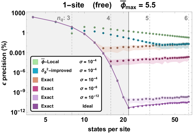
Figure 3: The precision of the ground state energy of the HO in Eq. (7) for unimproved, improved and exact conjugate-momentum operators, over a range of digitizations of $\bar{\phi}$ with different levels of gate noise. The light-green points correspond to implementing the finite-difference conjugate momentum operator, the light-blue corresponds to the ${\cal O}(\delta_{\tilde{\phi}}^{2})$-improved conjugate momentum operator, and the purple-points correspond to the exact conjugate momentum operator. Gaussian noise with a width $\sigma$ is added to the diagonal elements of the eigenvalues of the conjugate momentum operators (resembling a simplified version of process (3) in Fig. 1). The maximum value of the field is fixed to be $\bar{\phi}_{\rm max}=5.5$, enabling a precision of $\sim 10^{-12}$ for an ideal quantum computer. The vertical light-gray dashed lines correspond to the number of qubits associated with the number of states, while the solid darker-gray line corresponds to the naïve estimate of saturation of the NS sampling bound based upon the properties of the HO ground state wavefunction (the six calculations cross the latter of these lines top-to-bottom in the order of the legend). For the computational errors anticipated in the NISQ-era, 4 qubits are seen to be sufficient to eliminate the digitization of the scalar field as a source of important error.

IV.1.1 Perturbatively Improved Hamiltonian

It is interesting to note that terms can be added to the finite-difference conjugate-momentum operator $\tilde{\Pi}$ in Eq. (13) to systematically improve it by powers of $\delta_{\tilde{\phi}}^{2}$. Finding the improvement term is straightforward in conjugate-momentum space, which can then be transformed into $\tilde{\phi}$ space. By including appropriate terms to systematically cancel deviations from the true conjugate-momentum operator,

$$\hat{k}_{\tilde{\phi}}^{2} = {4\over\delta_{\tilde{\phi}}^{2}}\ \sin^{2}\left({k_{\tilde{\phi}}\ \delta_{\tilde{\phi}}\over 2}\right)\ \rightarrow\ k_{\tilde{\phi}}^{2}\ -\ {k_{\tilde{\phi}}^{4}\ \delta_{\tilde{\phi}}^{2}\over 12}\ +\ ...$$

$$\hat{k}_{\tilde{\phi}}^{\prime 2} = {4\over\delta_{\tilde{\phi}}^{2}}\ \sin^{2}\left({k_{\tilde{\phi}}\ \delta_{\tilde{\phi}}\over 2}\right)\ +\ {4\over 3\delta_{\tilde{\phi}}^{2}}\ \sin^{4}\left({k_{\tilde{\phi}}\ \delta_{\tilde{\phi}}\over 2}\right)\ \rightarrow\ k_{\tilde{\phi}}^{2}\ -\ {k_{\tilde{\phi}}^{6}\ \delta_{\tilde{\phi}}^{4}\over 90}\ +\ ...\ \ \ .$$ (18)

and the corresponding effective action can be derived that is parametrically improved. In $\tilde{\phi}$-space, the first term in this improvement is reproduced by an additional term in the Hamiltonian of the form,

$$\delta\tilde{H} = {1\over 24}\ \delta_{\tilde{\phi}}^{2}\ \tilde{\Pi}^{4}\ \ \ .$$ (19)

The quadratic improvement in the energy of the ground state of the HO due to the inclusion of this improvement term in the Hamiltonian is shown in Fig. 3. Numerical improvements on the order of one to two orders of magnitude in the accuracy of the improved calculations versus the unimproved calculations are found, and that the residual dependence on $\delta_{\tilde{\phi}}$ becomes ${\cal O}\left(\delta_{\tilde{\phi}}^{4}\right)$.

For systematic errors arising from approximation of the conjugate-momentum operator with a finite difference operator, the exact form of errors introduced into the Hamiltonian are well known. If the situation was not so fortunate, the polynomial digitization errors could still be systematically removed. Through a series of modest-sized calculations (in which $\bar{\phi}_{\text{max}}$ is chosen large enough) at a range of digitization scales, the leading polynomial dependence on the small parameter, $\delta_{\tilde{\phi}}$, may be calculated and removed through the introduction of additional Hamiltonian terms. While the form of such terms may be systematically informed perturbatively or by the simple availability of independent higher-dimension operators Weinberg (1979), their choice is not unique as the necessity is only to provide polynomial dependence at the correct order for cancellation. This follows the procedure of Symanzik improvement Symanzik (1983a); Sheikholeslami and Wohlert (1985); Luscher et al. (1996) as discussed at the end of Sec. II in the context of lattice QCD. Such improvement procedures are broadly applicable and have been crucial for calculating observables in lattice gauge theories—modestly increasing the complexity of the action rather than calculating closer to the continuum.

IV.1.2 The Impact of Noise

In the previous sections, we have considered a full non-perturbative improvement of the field conjugate-momentum operator implemented in field space through a QuFoTr, and a perturbative improvement that systematically eliminates increasing orders in the digitization introduced by finite-difference approximations of derivatives in field space. These correspond to different matrices for $\bar{\Pi}^{2}$ acting on the basis states in field conjugate-momentum space. The exact $\bar{\Pi}^{2}$ provides exponential precision in the low-lying eigenstates of the system, but deviations from this matrix may lead to only polynomial precision—as evidenced from the behavior of the perturbatively improved Hamiltonians and Fig. 3. Imperfect gates and decoherence will result in an imperfect application of $\bar{\Pi}^{2}$—introducing errors into calculations of observables and potentially making superfluous, at a practical level, the exponentially small improvements in digitization errors below the threshold of quantum noise.

In the presence of noisy gates and decoherence, it remains preferable to work with the exact $\bar{\Pi}^{2}$ operator, but the precision of its application is limited. For a given level of desired precision, the digitization and extent of the field basis required to ensure that the precision matches that of the noise can be determined. This would require an iterative tuning procedure in which multiple measurements are performed, systematically increasing $\bar{\phi}_{\rm max}$ and decreasing $\delta_{\tilde{\phi}}$ until the results of calculations become stable. These may or may not correspond to a situation that satisfies the NS sampling bound, depending upon the magnitude of the noise. In Fig. 3, the results of calculations are shown with the use of the unimproved, improved and exact conjugate-momentum operator through QuFoTr with the inclusion of different levels of gate-noise. The noise is included as an offset to each diagonal element of $\bar{\Pi}^{2}$ after QuFoTr from a Gaussian distribution of width $\sigma$ in conjugate-momentum space. The value of $\bar{\phi}_{\rm max}=5.5$ is chosen to allow for a precision of $\sim 10^{-12}$ for an ideal quantum computer for digitizations below a critical value of $\delta_{\tilde{\phi}}$. For a given gate-noise level, there is a value of $\delta_{\tilde{\phi}}$ below which smaller digitizations do not improve the precision of the calculation. The conclusion is that the error associated with digitization can be reduced below errors from other sources for an arbitrary number of low-lying energy eigenstates with only a small number of qubits.

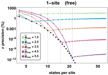
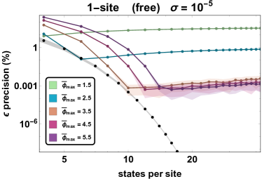
Figure 4: The precision of calculations of the ground state energy of the HO in Eq. (7). The left panel shows expectations for an ideal quantum computer for different values of $\bar{\phi}_{\rm max}$ as a function of the number of states. The vertical gray-dashed lines correspond to the location of inflection points predicted by the NS sampling theorem for the indicated values of $\bar{\phi}_{\rm max}$. A fit to the grey points calculated at the NS saturation point indicates $\epsilon\sim(1.8(2)\times 10^{3})\ 2^{-2.234(4)n_{s}}$, quantifying the double-exponential scaling between $\epsilon$ and $n_{Q}$. The right panel shows the expected precision from a device with noise at the level of $\sigma=10^{-5}$ in the application of the field conjugate-momentum operator (as described in the text). In both panels, the NS saturation points arise left-to-right in the top-to-bottom order of the legend.

The impact of different sampling ranges in $\bar{\phi}$ space upon the precision of calculations with an ideal quantum computer (perfect gates), is shown in the left panel of Fig. 4. The employed value of $\bar{\phi}_{\rm max}$ limits the overall precision of calculations as $\delta_{\tilde{\phi}}\rightarrow 0$ (states per site $n_{s}\rightarrow\infty$) due to under sampling of the field at large $\bar{\phi}$, which is suppressed by $\sim e^{-\phi^{2}/2}$ for a HO wavefunction. The field truncation also limits the precision of calculations for large values of $\delta_{\tilde{\phi}}$ due to under sampling of the field in momentum space. In between these regimes, the NS saturation point is found—perceived as a simple discontinuity in the first derivative—where the position-space sample rate becomes sufficient to capture the structure of momentum-space. Tracking this saturation point with the gray band of Fig. 4 shows a precision that increases exponentially in the number of states and thus double-exponentially in the number of qubits ($n_{s}=2^{n_{Q}}$). The coefficients of this precision scaling are calculated to be $\epsilon\sim(1.8(2)\times 10^{3})\ 2^{-2.234(4)n_{s}}$, which serves as a general estimate for qubit requirements to capture the low-energy Hilbert space of localized scalar fields.

An interesting observation that can be drawn from Fig. 3 is that, for the parameters of the calculations explored, reducing the amount of noise in the application of the field conjugate-momentum operator below $\sim 10^{-13}$ will have little impact on the precision of the extracted final result. The demonstration is made more concrete in the right panel of Fig. 4, where the noise level is fixed and the precision of calculations are determined over a range of $\bar{\phi}_{\rm max}$. For this noise level, there is no improvement in precision as $\bar{\phi}_{\rm max}$ is increased beyond $\sim 3.5$. These are simple special cases of a general conclusion, that for a given calculation designed with a set of digitization parameters, there is a level of noise in the quantum device(s) below which the precision of the results will be only minimally impacted. This general conclusion works in both directions and emphasizes the importance of matching precision in the qubit representation to that available from the NISQ hardware. Exceeding precision in either direction would result in a wasteful use of quantum resources—using extra qubits and gates to represent the physical system with a precision beyond the quantum hardware’s capability to resolve or using a noise-resilient quantum device to probe physics beyond that represented in the qubit representation of the system.

One plausible scenario in which it may be beneficial to exceed the precision of the quantum hardware with the qubit mapping is in the presence of post-measurement noise-mitigation techniques as shown for implementations of variational quantum eigensolvers in McClean et al. (2016); Kandala et al. (2017); Klco et al. (2018). By extrapolating in a parameter scaling with the noise of the system (in the NISQ-era, this is conventionally a number increasing with the number of two-qubit interactions), the precision of a calculation can be improved beyond the precision capable for any ensemble measurement with the device at a fixed noise parameter. In this case, it is the extrapolated precision of the quantum hardware that needs to be balanced with the theoretical precision of the qubit mapping in order to optimize the use of quantum resources.

It can be seen from Figs. 3 and 4 that the simple , yet physically-motivated, noise model implemented here does not significantly modify the results of calculations above the effective noise level. As has been shown for the use of momentum-space phases associated with finite difference field-space $\tilde{\Pi}^{2}$ operators in section IV.1.1, there exist simple modifications to the conjugate-momentum space phases that modify the precision convergence by introducing polynomial sources of error. Having now determined that gaussian random noise on conjugate-momentum space phase gates does not result in such a dramatic degradation of the calculation’s precision above the noise tolerance, we proceed with noiseless calculations—remembering that this property must be monitored as noise models become more accurate and relevant to specific hardware implementations.

IV.2 Harmonic Oscillator Basis

As we have discussed previously, any set of basis states can be used to digitize the field, $\bar{\phi}$, in $\bar{H}$ in Eq. (7). If the basis spans the $\bar{\phi}$-space and $\bar{\Pi}$-space of the lowest-lying eigenstates, the NS sampling theorem ensures exponential convergence to those eigenstates and associated eigenvalues. A basis that is commonly used, beyond the eigenstates of the $\bar{\phi}$ operator, is formed by a finite set of eigenstates of a HO with angular frequency $\omega_{\phi}$ that is tuned to optimize convergence in the number of states. If $\omega_{\phi}$ is tuned to $\omega_{\phi}=1$, the basis states are the eigenstates of $\bar{H}$ in Eq. (7) and the evolution matrix is diagonal in the basis, and the number of basis states required to converge to the lowest $N$ eigenstates is obviously equal to $N$. For $\omega_{\phi}\neq 1$, the basis states are not eigenstates, and the evolution matrix is not diagonal.

It should be emphasized that bases formed from HO eigenstates, that are explored in this section, are different in nature to those formed from digitized HO eigenstates, that have been considered previously Somma (2016); Macridin et al. (2018a, b). In those works, the eigenstates of the HO were digitized onto the eigenstates of the field operator, e.g. $\langle\bar{\phi}|\psi_{n}\rangle\rightarrow\langle\bar{\phi}_{i}|\psi_{n}^{d}\rangle$, reducing each field-space eigenstate from a continuous function to a discrete set. It was the properties and time-evolution of the $|\psi_{n}^{d}\rangle\sim\sum\limits_{i}\psi_{n}(\phi_{i})|\phi_{i}\rangle$ using the JLP framework that were examined in Refs. Somma (2016); Macridin et al. (2018a, b). A HO basis was also used in the pioneering calculations of the deuteron ground state energy using the IBM and Rigetti quantum hardware by an ORNL team Dumitrescu et al. (2018). The mapping of the system onto qubits was accomplished using a 2nd quantization framework, where occupancy of quantum states is encoded in the orientation of the qubit. In contrast, we consider a first quantized mapping with HO basis states mapped directly onto states of the quantum register.

Unlike the situation found with the JLP digitization of $\bar{\phi}$ in terms of eigenstates of the $\bar{\phi}$ operator, where it is valuable to QuFoTr into conjugate-momentum space to evaluate the exact action of $\bar{\Pi}^{2}$, digitization of the field space is accomplished explicitly by the HO basis with the coverage in field and conjugate-momentum spaces determined by the maximum number of basis states and the value of $\omega_{\phi}$. As such, quantum circuits implementing the action of the Hamiltonian in the HO basis can be constructed in $\bar{\phi}$ space only. The Hamiltonian and ladder operators defining the basis states are,

$$H_{\rm basis} = {1\over 2}\bar{\Pi}^{2}+{1\over 2}\omega_{\phi}^{2}\ \bar{\phi}^{2}\ =\ \omega_{\phi}\left(a_{\omega_{\phi}}^{\dagger}a_{\omega_{\phi}}+{1\over 2}\right)$$

$$a_{\omega_{\phi}} = \sqrt{\omega_{\phi}\over 2}\ \bar{\phi}+i\sqrt{1\over 2\omega_{\phi}}\bar{\Pi}\ \ ,\ \ a_{\omega_{\phi}}^{\dagger}\ =\ \sqrt{\omega_{\phi}\over 2}\ \bar{\phi}-i\sqrt{1\over 2\omega_{\phi}}\bar{\Pi}\ \ \ ,$$ (20)

and the Hamiltonian in Eq. (7) can be conveniently written in terms of the basis operators,

$$\bar{H} = {1\over 2}\bar{\Pi}^{2}\ +\ {1\over 2}\omega_{\phi}^{2}\bar{\phi}^{2}+{1\over 2}\left(1-\omega_{\phi}^{2}\right)\bar{\phi}^{2}\ =\ H_{\rm basis}\ +\ \delta H_{\omega_{\phi}}\ \ \ .$$ (21)

The eigenvalues and eigenstates of $\bar{H}$, in Eq. (7), are determined by diagonalizing the Hamiltonian matrix formed from matrix elements of $\bar{H}$ in a truncated basis of eigenstates of $H_{\rm basis}$, in Eq. (20). An explicit example of the HO basis for three qubits-per-site may be found in the Appendix Sec. C. Figure 5 shows the precision of calculations of the ground state energy of the HO Hamiltonian in Eq. (7) expected on an ideal quantum computer as a function of the size of the HO basis for different values of $\omega_{\phi}$.

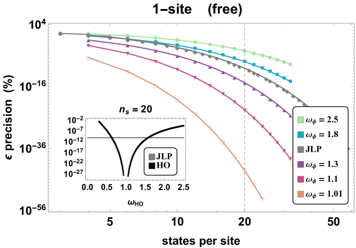
Figure 5: The expected precision of the ground state energy of the HO Hamiltonian in Eq. (7) on an ideal quantum computer using a HO basis defined by $\omega_{\phi}$ in Eq. (20) as a function of the number of basis states. The inset figure shows the scaling for a HO basis of 20 states, which is a slice of the main figure indicated by a vertical gray dashed line (the calculations cross this line top-to-bottom in the order of the legend). In the limit of $\omega_{\phi}=1$ the lowest-lying basis state is an eigenstate, and $\epsilon=0$. Tuning $\omega_{\phi}$ to be in the vicinity of the optimal value $\omega_{\phi}=1$ outperforms field-space digitization, shown by the gray JLP curve.

Obviously, when $\omega_{\phi}=1$ the error vanishes. For $\omega_{\phi}$ tuned to be in the vicinity of $\omega_{\phi}=1$ the precision obtained with the HO basis is better than that obtained with field-space digitization discussed in the previous sections. However, poor choices of $\omega_{\phi}$ lead to inferior precision compared with field-space digitization.

The time-evolution induced by $H_{\rm basis}$ is simple, involving only single-phases, and the quantum circuit to implement it corresponds to only phases applied to each qubit. Since there are no interactions in this basis, all operators commute and there is no need for a Trotter decomposition, as the total phase can be determined and applied in one application. When detuned away from $\omega_{\phi}=1$, the size of the Trotter step required to time-evolve the system will be determined by the detuning. In such a detuned scenario, the operator structure from $\delta H_{\omega_{\phi}}$ involves interactions between all qubits, as evidenced from Eq. (39).

Basis	$n_{Q}$	0-body	1-body	2-body	3-body	4-body	5-body	6-body	$QFT$	CNOTs
	2	1	8	2					$\checkmark$	8
	3	1	14	6					$\checkmark$	24
JLP	4	1	20	12					$\checkmark$	48
	5	1	26	20					$\checkmark$	80
	6	1	32	30					$\checkmark$	120
JLP	$n_{Q}$	1	$6n_{Q}-4$	$2*\binom{n_{Q}}{2}$					$\checkmark$	$8\binom{n_{Q}}{2}$
	2	1	2							0
	3	1	3							0
HOω≡1	4	1	4							0
	5	1	5							0
	6	1	6							0
HOω≡1	$n_{Q}$	1	$n_{Q}$							0
	2	1	3	1						2
	3	1	4	4	3					20
HOω≠1	4	1	5	5	11	7				96
	5	1	6	6	16	26	15			352
	6	1	7	7	22	42	57	31		1120

Table 1: Resource requirements for one step in the Trotterized time evolution of a HO in the field-digitization JLP basis, a tuned HO basis, and a detuned HO basis. CNOT counts are based upon a standard multi-Pauli implementation requiring $2(k-1)$ CNOTs for each $k$-body operator. When a QuFoTr is required (JLP), the standard CNOT counts of $2\binom{n_{Q}}{2}$ for this operation (and its inverse) are included. With the expected limitations in the number of gate operations applied in NISQ-era devices, only systems with $n_{Q}\leq 4$ may be practical.

In Table 1, comparisons in the types and numbers of operations and gates required to time-evolve the HO described by $\bar{H}$ in Eq. (7) between the field-digitization basis and a tuned/detuned HO basis are presented. The 2-qubit, CNOT gate requirements are distinguished separately as their presence often represents the largest source of noise on NISQ-era quantum hardware. The numbers in Table 1 are accumulated for a standard implementation of multi-Pauli gates Nielsen and Chuang (2011) and do not represent expected reductions of the HO basis operations through parity calculation or cancellations that may occur for particular choices of the operator ordering Hastings et al. (2015). From Table 1, it is clear that a tuned HO basis requires significantly fewer operations to evolve a free HO than does the field-digitization basis. This is because the eigenstates of the system correspond exactly to the basis states. However, a detuned HO basis involves an exponentially-growing number of multi-qubit operations, leading to significantly more operations than the field-digitization basis. Even when the eigenbasis is unknown, JLP has resource requirements limited to 2-body operators. As a detuned HO basis shares features of a self-interacting system (detailed subsequently), we conclude that, for this very simple system, the field-digitization basis examined in detail in the works of JLP is more robust than a generic HO basis. By this, we mean that for the evolution of an arbitrary, apriori unknown system, the field-digitization basis will typically require fewer quantum computational resources while possibly requiring fewer qubits, as seen from Fig. 5.

It is interesting to consider whether the tuned HO could be used as a “standard candle” for the calibration of quantum hardware. Its eigenstates and eigenenergies are known to infinite precision and thus could be considered not only as a calibration source but also as a calculation to distinguish the computational precision capable on classical and quantum hardware. Using the details above and specifically the information of Table 1, it can be seen that the tuned HO requires 0 two-qubit gates to implement. As such, it contains no entanglement and thus no unique signal that could not be generated with other pre-determined rotation gates to quantify and explore noise in NISQ-era hardware.

IV.3 $\lambda\phi^{4}$ Scalar Field Theory: Comparing Bases

After the field and Hamiltonian redefinition of Eq. (7), the interacting 0+1 scalar field is described by,

$$\bar{H} = {1\over 2}\bar{\Pi}^{2}+{1\over 2}\bar{\phi}^{2}+\frac{\bar{\lambda}_{0}}{4!}\bar{\phi}^{4}\ \ \ ,$$ (22)

where $\hat{\phi}={1\over\sqrt{\hat{m}_{0}}}\bar{\phi}$, $\hat{\Pi}=\sqrt{\hat{m}_{0}}\bar{\Pi}$, $\hat{H}=\hat{m}_{0}\bar{H}$, and $\hat{\lambda}_{0}=\hat{m}_{0}\bar{\lambda}_{0}$. This system has been numerically studied previously by Somma Somma (2016). A value of $\bar{\lambda}_{0}=32$ will be chosen as a representative case of strong coupling, where the system is no longer a HO (nor perturbatively close) and the basis selection for the description of the wavefunction between JLP digitization and HO basis functions is relevant within the multi-dimensional space of precision, qubits, gate decompositions, and tuning requirements.

When using the digitization techniques of JLP, introducing additional interactions does not introduce new challenges. The only necessary modifications to the method are rescalings of the sampling distributions (applying considerations for both field and conjugate-momentum space coverage).

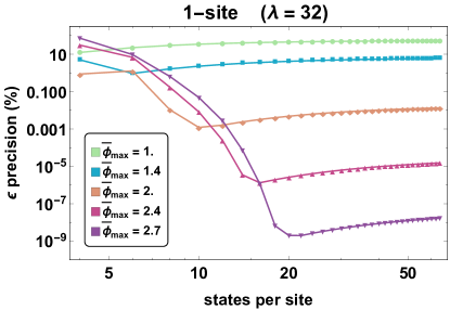
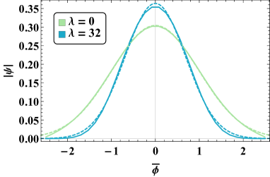
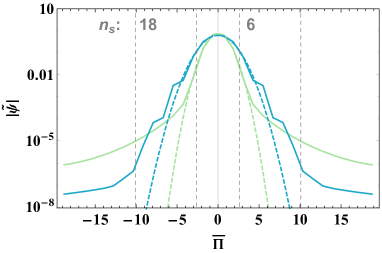
Figure 6: The panel in the upper row shows the expected precision of calculations of the ground-state energy of a 1-site $\lambda\phi^{4}$ scalar field theory performed with an ideal quantum computer for different values of $\bar{\phi}_{\rm max}$ as a function of the number of states (the NS saturation points arise left-to-right in the top-to-bottom order of the legend). The lower row shows the field and conjugate-momentum space wavefunctions (left and right, respectively) for the free(green or lightly-shaded) and interacting(blue or darkly-shaded), 1-site $\lambda\phi^{4}$ shown at constant $\bar{\phi}_{\rm max}=2.5$. The introduction of non-zero $\lambda$ reduces the spatial support of the wavefunction while increasing its support in momentum space. The small-dashed green(lightly-shaded) and blue(darkly-shaded) lines in the right panel are Fourier transforms of Gaussian fits to the wavefunctions in the left panel. The vertical, gray dashed lines in the right panel show the truncations in $\bar{\Pi}$ for 6 and 18 states—the location of NS saturation for $\bar{\phi}_{\rm max}=2.5$ as seen in Figs. 4 and the first row here.

In the case of $\lambda\phi^{4}$ with $\lambda=32$, introduction of the self-interaction shrinks the domain over which the wavefunction has support as shown in the lower left panel of Fig. 6. As a result, smaller values of $\bar{\phi}_{\rm max}$ may be used for precise calculations. This can be seen in a comparison between Fig. 4 and the upper panel of Fig. 6. For a $\bar{\phi}_{\rm max}$ of 2.5, the highest precision attainable with $\lambda=0$ and $\lambda=32$ differs by $\sim 5$ orders of magnitude. The precision with $\bar{\phi}_{\rm max}$ of 2.5 saturates with 18 states for $\lambda=32$, but saturates with only 6 states for $\lambda=0$, indicating that the value of $\bar{\Pi}_{\rm max}$ has also increased with the introduction of the self-interaction, requiring a smaller value of $\delta_{\tilde{\phi}}$ in order to accurately represent the enlarged Fourier space. This trade-off can be seen in the lower-right panel of Fig. 6. To capture the Gaussian structure of the free HO requires only the inclusion of a small region of $\bar{\Pi}$ around zero. For 6 states, the maximum value of the momentum can be determined by Eq. (15) to be $\pm 2.62$. This value is indicated by the vertical, gray dashed lines in Fig. 6. Outside of this region, the exponential behavior turns power-law and inclusion of this portion of the wavefunction no-longer informs the sampling about the physical momentum space, only about artifacts of the truncation. By fitting a continuous Gaussian of infinite spatial extent to the wavefunction at left and plotting its Fourier transform on the right (small-dashed curves), 6 states are found to lead to a $\delta_{\tilde{\phi}}$, and thus a maximum $k_{\tilde{\phi}}$, that captures the Gaussian central region of the wave function. For $\lambda=32$, this maximum value in momentum space is no longer sufficient to saturate the NS sampling limit. There is a significantly larger domain in momentum space before the wavefunction transitions to power-law behavior, not appearing until $\bar{\Pi}$ values of $\sim\pm 10$. Again, with Eq. (15), 18 states per site are seen to be required for this truncation in momentum space, a value in agreement with the location of the NS saturation point seen in the upper panel of Fig. 6.

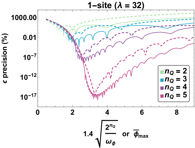
Figure 7: Exploration of sensitivity in JLP field digitization (dashed lines) and the HO basis (solid lines) to tuning of digitization parameters determining the low-energy states in momentum space. For JLP, the relevant parameter is $\bar{\phi}_{\rm max}$, while for the HO basis it is a combination of the frequency defining the basis, $\omega_{\phi}$ and the number of states, $\sim\sqrt{2^{n_{Q}}/\omega_{\phi}}$. The horizontal axes of the HO curves have been rescaled to $1.4\sqrt{2^{n_{Q}}/\omega_{\phi}}$ to align them with the JLP curves. These tuning curve pairs are minimized with smaller values of $\epsilon$ in the top-to-bottom order of the legend.

By comparing the gray band in Fig. 4, the scaling of the NS saturation for the free 1-site HO, with the highest precisions attained in the upper panel of Fig. 6, it can be seen that the number of states (or qubits) required to achieve a particular precision is relatively stable for this self-interaction. The values of $\bar{\phi}_{\rm max}$ along this band are skewed from those in the free theory, but the maximum precision attained through distribution of a fixed number of wavefunction sample points is not. As this self-interaction causes a smooth deformation of the wavefunction, trading extent in field space for that in conjugate-momentum space, it is not surprising that the interacting ground state wavefunction achieves similar precision given similar quantum resources.

When using a basis of HO wavefunctions, the main consideration is, again, assuring that the chosen representation of the wavefunction sufficiently spans both field and conjugate-momentum space. With JLP, $\bar{\phi}_{\rm max}$ is used to control the domain of support in field space while $\delta_{\tilde{\phi}}$ (or equivalently the number of states per site) is used to control the domain of support in momentum space. With the HO basis functions, the parameters to be tuned are $\omega_{\phi}$ and the number of states. Unlike the lattice-parameters of JLP, these parameters give correlated modifications to field and conjugate-momentum space. Increasing $\omega_{\phi}$ creates basis functions that are more localized in field space while exploring higher momentum-space truncations. Increasing the number of states also increases the momentum-space truncation, but expands the field-space region of support. Because of these correlations, it is meaningful to compare JLP’s dependence of $\bar{\phi}_{\rm{max}}$ with a combination of $n_{Q}$ and $\omega_{\phi}$ dictating the extent of the HO wavefunction basis, $\sqrt{\frac{2^{n_{Q}}}{\omega_{\phi}}}$, reflecting the fact that $\sqrt{\langle\phi^{2}\rangle}\sim\sqrt{2^{n_{Q}}}$ and $\sim 1/\sqrt{\omega_{\phi}}$.

Basis	$n_{Q}$	0-body	1-body	2-body	3-body	4-body	5-body	6-body	$QFT$	CNOT${}_{\text{uncompiled}}$	CNOT${}_{\text{compiled}}$
	2	1	8	2					$\checkmark$	8	8
	3	1	14	6					$\checkmark$	24	24
JLP	4	1	20	12		1			$\checkmark$	54	52
	5	1	26	20		5			$\checkmark$	110	96
	6	1	32	30		15			$\checkmark$	210	164
JLP	$n_{Q}$	1	$4n_{Q}-6$	$2*\binom{n_{Q}}{2}$		$\binom{n_{Q}}{4}$			$\checkmark$	$8\binom{n_{Q}}{2}+6\binom{n_{Q}}{4}$
	2	1	3	2						4
	3	1	5	9	4					34
HO	4	1	6	16	18	10				164
	5	1	7	22	32	44	22			612
	6	1	8	29	44	84	98	46		1982

Table 2: Resource requirements for one first-order-Trotterized step of time evolution for 1-site $\lambda\phi^{4}$ scalar field theory in the field-digitization JLP basis and HO basis. CNOT counts are based upon a standard multi-Pauli implementation requiring $2(k-1)$ CNOTs for each $k$-body operator. When the QFT is required (JLP), the standard CNOT counts of $2\binom{n_{Q}}{2}$ for this operation (and its inverse) are included in the second-to-last column. The last column contains the required CNOT gates after manual compilation (see Appendix B). With the expected limitations in the number of gate operations applied in NISQ-era devices, only systems with $n_{Q}\leq 4$ may be practical.

In Fig. 7, the expected precision of the ground-state energy is shown as a function of $\bar{\phi}_{\rm max}$ and $\sqrt{\frac{2^{n_{Q}}}{\omega_{\phi}}}$ for JLP (dashed) and HO (solid) bases, respectively. Values on the left of the minimum of each curve have reduced precision due to insufficient sampling in field space, while to the right of the minimum, the precision is reduced due to insufficient sampling in momentum space. Only at the minimum is the sampling in both spaces optimal. It can be concluded that for these parameters, values of $\bar{\phi}_{\rm max}$ or $\omega_{\phi}$ can be selected (for $n_{Q}\geq 3$) such that the errors introduced by digitization are significantly smaller than those expected from computations on NISQ-era hardware. As such, the digitization of the scalar field is not expected to limit the accuracy of NISQ-era computations. For $n_{Q}<3$, the field digitization is expected to provide a limit to the accuracy of NISQ-era computations. Comparing the basis choices given a fixed number of qubits, there is a value of the HO basis parameters that produce a higher-precision result in this system than a $\bar{\phi}_{\rm max}$-tuned JLP wavefunction digitization. For a desired precision, the HO basis offers a larger acceptable window in the basis tuning parameters than does the JLP field digitization basis. This translates, through the circuit descriptions of Figs. 12 and 14, to reduced sensitivity on the exact angles applied in the Z-axis rotation gates. This sensitivity will be relevant in the NISQ era with imperfect gate fidelities, and will continue to be relevant once fault-tolerant quantum computing is available (where the precision determines the number of $T$ gates  needed to decompose any Z-axis rotation with expected scaling of $\big{|}\log_{2}|\epsilon_{\theta}|\big{|}$ Selinger (2015); Ross and Selinger (2016); Kliuchnikov et al. (2013). )

While Fig. 7 shows desirable qualities when using HO basis functions to digitally describe the wavefunction, quantum simulations of quantum systems have many resource requirements to consider beyond qubit number and necessary precision of rotation angles. Specifically, a large consideration in the feasibility of successfully implementing a quantum calculation in the NISQ era is the number and type of gates required to implement a single Trotter step of the time-evolution operator. These gate counts are detailed in Table 2. For JLP, the 1-body operators from the QFT and $\binom{n}{2}$ 2-body operators from the terms quadratic in the field and its conjugate momentum are still present. The $\lambda\phi^{4}$ interaction term introduces only $\binom{n}{4}$ 4-body operators and additional contributions to the identity and 2-body operators. The latter can be consolidated with the operators previously identified and thus does not contribute to the gate cost (it does, however necessitate separate operator coefficient structures in field and conjugate-momentum space, e.g., $\mathcal{O}_{0}$ from Eq.(26) can be written as $\mathcal{O}_{\tilde{\Pi}}$ and $\mathcal{O}_{\tilde{\phi}}$ which contain the same operators but with different relative coefficients). The fact that operators are limited to interacting between a number of qubits equal to the highest power of field interaction included in the Hamiltonian is a feature of JLP not shared by the HO basis. Here, the additional 2-qubit CNOT gates required to implement the QuFoTr for JLP field digitization are quickly outnumbered by the CNOT gates required to implement the $k$-body operators for $k$ limited by the number of qubits in the site-register.

The fact that the scaling of CNOTs in the JLP basis is limited to $n_{Q}^{4}$ is advantageous when considering the noise landscape of NISQ-era hardware dominated by 2-qubit interactions. In Table 1 and Table 2, the CNOT gate counts generally do not include cancellations that may occur for particular operator orderings in the Trotterization Hastings et al. (2015). In the JLP basis, we have performed a manual circuit compilation of the $\lambda\phi^{4}$ scalar field theory, eliminating pairs of adjacent CNOT gates, resulting in the CNOT gate counts shown in the right-most column of Table 2. While the $\bar{\phi}^{2}$ operator set by itself does not permit a reduction of the number of gates, in combination with the $\bar{\phi}^{4}$ operator set, and also among the $\bar{\phi}^{4}$ operators, redundant CNOT operations in the leading Trotter expansion can be removed. While a similar reduction can be applied to the circuits of the HO basis, many changes of Pauli bases between operations make systematic cancellation difficult. As was the case with the JLP basis, it is not expected that carrying out this elimination in the HO basis will change the scaling of the CNOT-operator accumulation. A discussion of this manual compilation is given in Appendix B.

IV.3.1 Delocalized Wavefunctions: $m^{2}<0$

As mentioned in the introduction, $\lambda{\bm{\phi}}^{4}$ scalar field theory in $3+1$ dimensions is a cornerstone of the standard model of electroweak interactions Glashow (1961); Weinberg (1967); Salam (1968), where ${\bm{\phi}}$ is an electroweak doublet of complex real scalar fields. At low energies, its potential is such that the vev of $\langle{\bm{\phi}}\rangle\neq 0$, breaking the electroweak gauge group SU(2)${}_{L}\otimes\text{U(1)}_{Y}\rightarrow\text{U(1)}_{Q}$ down to that of quantum electrodynamics. This minimal symmetry-breaking mechanism, the Higgs mechanism, generates masses for the weak gauge bosons and the fermions, and gives rise to a single physical scalar particle, the Higgs boson Higgs (1964); Englert and Brout (1964); Aad et al. (2012); Chatrchyan et al. (2012).

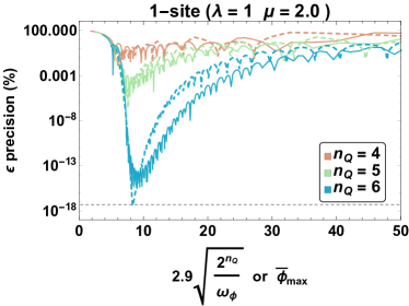
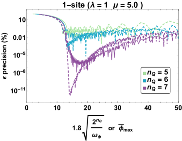
Figure 8: Exploration of the sensitivity in JLP field digitization (dashed lines) and the HO basis (solid lines) to tuning of digitization parameters determining the low-energy states for a 0+1-dimensional scalar field theory with $m^{2}<0$, with $\mu=2$ (left panel) and $\mu=5$ (right panel), resulting in delocalized wavefunctions. For JLP, a relevant parameter is $\bar{\phi}_{\rm max}$, while for the HO basis it is a combination of the frequency defining the HO basis, $\omega_{\phi}$, and the number of states per site. The horizontal axes of the HO curves have been rescaled to $2.9\sqrt{2^{n_{Q}}/\omega_{\phi}}$ in the left panel and $1.8\sqrt{2^{n_{Q}}/\omega_{\phi}}$ in the right panel to align them with the JLP curves. The black-dashed horizontal line in the left panel corresponds to the precision required to distinguish between the ground state and $1^{st}$ excited state for $\mu=2$. The corresponding line for $\mu=5$ in the right panel lies many orders of magnitude beyond the range of the figure. In both panels, the tuning curve pairs are minimized with smaller values of $\epsilon$ in the top-to-bottom order of the legend.

In a 0+1 dimensional theory, the parameter regime $-\mu^{2}=m^{2}<0$ produces a potential that contains two minima located at $\phi=\pm\frac{\sqrt{3!}\mu}{\sqrt{\lambda}}$. For any physical value of $\mu$, the ground state wavefunction of the Hamiltonian is symmetric under $\phi\rightarrow-\phi$ and non-degenerate and, as such, respects the discrete global $Z_{2}$ symmetry of the Hamiltonian, with a vev of $\langle\phi\rangle=0$. However, it is delocalized with maxima near the two minima of the potential. The wavefunction of the $1^{st}$-excited-state of the system is similar to that of the ground state, but it is antisymmetric under $\phi\rightarrow-\phi$. As $\mu$ becomes large, and the components of both wavefunctions become increasingly localized around the minima of the potential, the energy difference between the ground state and the $1^{st}$-excited-state becomes exponentially small, determined by the barrier-penetration amplitude for transitioning from $+\phi$ to $-\phi$.

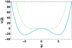
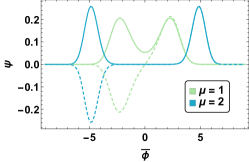
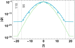
Figure 9: The potentials (left panel) and wavefunctions (center and right panels) of the ground states (solid curves) and $1^{st}$ excited states (dashed curves) for systems with $m^{2}<0$. The center panel shows the spatial wavefunctions for $\lambda=1$ and $\mu=1,2$, while the right panel shows the corresponding momentum-space wavefunctions. These wavefunctions result from using the JLP basis with $\overline{\phi}_{\rm max}=9$ and $n_{Q}=7$ qubits. (The vertical dashed-grey lines in the right panel indicate the number of states at which the NS bound is saturated and thus an increase in $\bar{\phi}_{\rm max}$ would be profitable over an increase in quantum states).

It is again relevant to consider alternate digitizations for representing the distributions in field and conjugate-momentum space. For large $\mu^{2}>0$, (where the quantity $\frac{\mu}{\sqrt{\lambda}}$ is large with respect to the wavefunction’s natural spatial extent), the field space wavefunction expands toward two localized and distinct regions of support. This is the case for the parameter values of $\mu=2,5$ and $\lambda=1$ chosen in Fig. 8 and in Fig. 9. This enlarged field-space coverage demands similarly-large values of $\bar{\phi}_{\rm max}$ when working in the JLP digitization, or smaller values of $\omega_{\phi}$ in defining the HO basis. Achieving these requirements can be accomplished in either basis when they are tuned, as shown in Fig. 8. An additional consideration in considering the configuration of quantum simulations is that the $1^{st}$-excited-state is becoming very close in energy with the ground state, a feature that is not present in the previously considered situations. A low-precision calculation, resulting from the use of a small number of qubits, will be unable to resolve the ground state from the $1^{st}$-excited-state, and the wavefunctions emerging from such calculations will likely be arbitrary combinations of the two. Higher-precision calculations, requiring a larger number of qubits, will be required to resolve the low-lying states in such systems. For such delocalized states, in contrast to the results obtained from a potential with $m^{2}>0$ in Fig. 7, the JLP basis can be tuned to produce higher precision in the ground-state energy than the HO basis with the same number of qubits. This outcome is not surprising—if the wavefunction is deformed into a distribution that is far from Gaussian, as seen in Fig. 9, a set of HO basis functions is no longer expected to offer superior coverage in the digital sampling. An interesting result of this demonstration is the degree to which the formulation of JLP, in which the basis is a periodic collection of delta functions agnostic to the structure of the wavefunction, is capable of exceeding the precision of a basis specialized for an alternate symmetry of the low-lying wavefunctions. The ability of JLP to perform with precision when applied to a range of systems, and thus require little knowledge of the structure of the low-lying states, will be a desirable feature of quantum simulations of more sophisticated, strongly-interacting field theories.

In these types of systems, and others, with near-degenerate low-lying states, the impact of noise in the quantum device upon correctly identifying the ground state wavefunction is expected to be significant. As discussed in Appendix H, the noise levels (from either the propagator approximation of step (2) or the intrinsic gate implementation noise of step (3) in Fig. 1) present in calculations with multiple degenerate extrema in the potential producing delocalized low-lying states will limit the systems that can be reliably explored as energy splittings are buried below the software (2) and hardware (3) noise levels.

V 1+1 Dimensional $\lambda\phi^{4}$ Scalar Field Theory

The detailed analysis of $0+1$ scalar field theory presented in the previous sections provides a solid foundation with which to consider scalar field theory in higher spatial dimensions with NISQ-era quantum computers. In section II, the Hamiltonian for scalar field theory in $d+1$ dimensions was presented, along with its naïve layout on a spatial lattice. The operator structure for multiple spatial sites is the same as for one spatial site except for the presence of the $\phi\nabla^{2}\phi$ operator, which includes contributions from particle motion into the Hamiltonian. The naïve representation of this operator as $\phi\nabla_{a}^{2}\phi$ introduces terms that couples the fields at two adjacent spatial sites. In general, smearing the fields to tame high-energy quantum fluctuations, while preserving low-energy observables, will introduce couplings beyond adjacent spatial sites, but these can be implemented with operations on two sites also.

In the situation with $d>0$, the text-book way to construct field theory calculations is to work with HO’s for each spatial-momentum mode, i.e. define fields in terms of quanta with well-defined spatial momentum. In perturbative calculations that can be performed by hand, this method is extremely efficient. In numerical computations of non-perturbative field theories, such as LQCD, the system is typically defined with regard to fields in position space, while components of calculations involve determining eigenvectors of the Dirac operator in the presence of a particular configuration of gauge fields. In the study of systems with few sites in each spatial direction, it is likely the case that calculating with the momentum-space modes is efficient Yeter-Aydeniz and Siopsis (2018). First implementation of this quantization procedure on quantum devices has been completed by an ORNL team Yeter-Aydeniz et al. (2019). However, as argued by JLP Jordan et al. (2011, 2012, 2014, 2018), as the interactions that are local in position space, such as $\lambda\phi^{4}$, become non-local in momentum space (distant momentum oscillators are capable of producing momentum-conserving contributions to the Hamiltonian), time evolving the system to a given state defined in momentum-space will become increasingly inefficient with increasing system size relative to a state defined in position space Jordan et al. (2011, 2012, 2014, 2018); McClean et al. (2014). For the remaining discussion, we will limit ourselves to states and operations defined in position space.

Figure 10: The ground and first-excited state wavefunctions for 2-site $\lambda\phi^{4}$ scalar field theory with $\lambda=0$ and $\lambda=32$ (top and bottom, respectively). The first excited state shows positive correlation between the oscillations at the two spatial sites $\left(\bar{\phi}_{0},\bar{\phi}_{1}\right)$.

Application of the $d+1$-dimensional $\lambda\phi^{4}$-Hamiltonian time evolution operator to a position-space state can be accomplished site-by-site, and involve at most $d$ neighboring two-site interactions at each site. Therefore, for a system with $\left(L/a\right)^{d}$ spatial lattice sites, this will require $\left(L/a\right)^{d}$ such applications. This being the case, study of the 2-site $1+1$ dimensional $\lambda\phi^{4}$ theory provides a complete inventory of the operations and gate counts required to perform a $d+1$-dimensional $\lambda\phi^{4}$ calculation, and we have performed such estimates and numerical calculations in this 2-site theory. Given this 2-site locality and quantum hardware capable of parallelizing the implementation of gates acting in separate tensor product spaces, application of the Hamiltonian to a position-space state can be accomplished with a circuit of constant depth with increasing lattice size Lloyd (1996). The field-space wavefunctions associated with the ground state and first-excited state of the 2-site $1+1$ dimensional theory are shown in Fig. 10, with the wavefunction at site-0 denoted by $\bar{\phi}_{0}$ and at site-1 by $\bar{\phi}_{1}$. A large value of the self-interaction coupling, $\lambda$, focuses this correlation in $\left(\bar{\phi}_{0},\bar{\phi}_{1}\right)$.

Figure 11: The precision of the calculated ground-state energy for the 2-site lattice $\lambda\phi^{4}$ scalar field theory with $\lambda=32$ performed with an ideal quantum computer for different numbers of qubits as a function of support in field space. For JLP, the relevant parameter is $\bar{\phi}_{\rm max}$, while for the HO basis it is a combination of the frequency defining the HO basis, $\omega_{\phi}$, and the number of states per site. The shown precision does not include deviations of this 2-site $1+1$ dimensional theory from the continuum limit of the $1+1$ dimensional theory for which the number of spatial sites approaches infinity for a fixed spatial extent. The horizontal axes of the HO curves have been rescaled to $1.4\sqrt{2^{n_{Q}}/\omega_{\phi}}$ to align them with the JLP curves. These tuning curve pairs are minimized with smaller values of $\epsilon$ in the top-to-bottom order of the legend.

As seen in Fig. 11, the 2-site $\lambda\phi^{4}$ theory experiences double-exponential convergence in $n_{Q}$ to the un-digitized value. However, just as the use of a finite-difference operator in the field-space implementation of $\bar{\Pi}^{2}$ introduced polynomial deviations in $\delta_{\bar{\phi}}$ (see results from local and improved operators in Fig. 3), the finite-difference implementation of $\phi\nabla_{a}^{2}\phi$ in position space introduces analogous polynomial deviations in $a$ from the continuum limit. These lattice-spacing errors are not shown in Fig. 11. Thus, this method converges to the continuum value with lattice-spacing errors that scale as $\epsilon\sim 2^{N_{Q}}$. Of course, with a large quantum computer, it could become possible to remove these polynomial lattice-spacing artifacts through use of the QuFoTr and subsequent implementation of the exact lattice phases in Fourier space to create a smeared, non-local gradient operator (exactly as was done in field space). Rather than requiring a QuFoTr to be applied on each of the modest-sized qubit registers associated with individual lattice sites, this proposal would require a QuFoTr across the entire lattice—an entangling operation amongst all $N_{Q}$ qubits. At least in the NISQ era, it is expected that such global operations will be prohibitive both in gate fidelity as well as coherence time. For this reason, the finite-difference form of the gradient operator, demanding only local interactions between the qubit registers at neighboring sites, appears to be optimal Jordan et al. (2011, 2012, 2014, 2018).

Basis	$n_{Q}$	2-body	3-body	4-body	5-body	6-body	7-body	8-body	9-body	10-body	11-body	12-body	CNOT
	2	4											8
	3	9											18
JLP	4	16											32
	5	25											50
	6	36											72
	$n_{Q}$	$n_{Q}^{2}$											$2n_{Q}^{2}$
	2	1	6	9									80
	3	1	8	30	56	49							1,152
HO	4	1	10	47	140	271	330	225					11,264
	5	1	12	68	244	630	1204	1668	1612	961			89,600
	6	1	14	93	392	1186	2772	5154	7560	8541	7182	3969	626,688

Table 3: Operators associated with the additional $\bar{\phi}(x)\bar{\phi}(x+1)$ operator resulting from the finite-difference spatial gradient operator $\phi\nabla_{a}^{2}\phi$ for time evolution of 2-site lattice $\lambda\phi^{4}$ scalar field theory in the JLP and HO field-digitization bases. CNOT counts are based upon a standard multi-Pauli implementation requiring $2(k-1)$ CNOTs for each $k$-body operator.

When implementing the gradient operator as a finite difference, there is only one set of operators $\bar{\phi}(x)\bar{\phi}(x+1)$ acting between the spatial sites that need be additionally considered. Table 3 shows the nature and number of pauli terms associated with this additional operator in the $1+1$-dimensional Hamiltonian. In this 1+1-dimensional system, the coefficient of the mass term in field space is modified by two of the terms in the $\phi\nabla_{a}^{2}\phi$ operator, but the operator structure is unaltered. As mentioned above, the quantum resources calculated in this paper may be easily combined to determine the requirements for larger lattices in $d$-dimensions, for example

$${\rm CNOT}_{lattice}(n_{Q},d,L/a)=L^{d}a^{-d}\ {\rm CNOT}_{\text{1-site}}(n_{Q})+dL^{d}a^{-d}\ {\rm CNOT}_{\bar{\phi}(x)\bar{\phi}(x+1)}(n_{Q})$$ (23)

expresses the total number of CNOT gates required to evolve the field across a lattice with CNOT${}_{\text{1-site}}(n_{Q})$ extracted from Tables 1 or 2 for the free or self-interacting fields, respectively, CNOT${}_{\bar{\phi}(x)\bar{\phi}(x+1)}(n_{Q})$ extracted from Table 3, $n_{Q}$ the number of qubits used to digitize the field at each site, $d$ the dimensionality of space, $L$ the spatial extent in each dimension, and $a$ the lattice spacing in each dimension. The nearest-neighbor interactions between sites in the JLP digitization requires all $n_{Q}^{2}$ 2-body operators that can be created between the two site registers. This is contrasted by the HO basis where operators between the two site registers are not limited to 2-body qubit interactions, but require tensor product Pauli operators acting on up to all $2n_{Q}$ qubits. Because of this dramatic difference in the structure of necessary operators, even for the smallest number of qubits per spatial site, the JLP basis requires fewer resources to implement the $\phi\nabla_{a}^{2}\phi$ operator—emphasizing the importance of an application’s physical representation onto qubit degrees of freedom in quantification of its required quantum resources.

VI Summary and Outlook

Quantum computing and quantum information science is anticipated to provide disruptive changes to scientific computing and to the ways that we think about addressing scientific challenges. The prospect of being able to explore quantities in quantum many-body systems, including quantum gauge field theories such as quantum chromodynamics, that require exponentially-large classical computing resources, such as for dense matter or in the time-evolution of non-equilibrium systems, is truly exciting. In this work, we have built upon foundational works by Jordan, Lee and Preskill Jordan et al. (2011, 2012, 2014, 2018) on how to formulate scalar field theory on quantum computers to determine properties of the scalar particle and interactions, both elastic and inelastic, between particles. In an attempt to understand the magnitude of resources required for even modest quantum computations in a simple field theory, our work has focused on the digitization of scalar field theories with only a small number of qubits per spatial lattice site. The recent work by Macridin, Spentzouris, Amundson and Harnik Macridin et al. (2018a, b), which, building upon the work of Somma Somma (2016), emphasized the utility of the Nyquist-Shannon (NS) sampling theorem, is a theme for our work as it provides an important guide for tuning digitization parameters in quantum field theories for the accurate representation of field and conjugate-momentum spaces on quantum devices (and may also have implications for classical calculations).

In addition to an in-depth exploration of the requirements for a basis of eigenstates of the field operator, as introduced by JLP, we have introduced and explored the resources required for, and the utility of, a basis of harmonic oscillator eigenstates. We have performed operator decompositions of the Hamiltonians for a small number of qubits in $0+1$ and $1+1$ dimensional systems. As tunings are required in both bases for an optimal computation on an ideal quantum device, we find that both bases are effective, but that the JLP basis appears to be more robust for systems that are delocalized in field space or not smooth in either field or conjugate-momentum space. We considered the impact of noise on calculations in such systems and found that parameters defining the field theory should be tuned given the limits in precision imposed by the quantum device in order to optimize the scientific productivity of the calculation. In either basis, when tuned, a quantum device with $n_{Q}=3$ or $n_{Q}=4$ qubits used to define the field at each spatial lattice site is found to be able to provide a precision of better than $\sim 10^{-6}$ for a given lattice spacing for a potential with $m^{2}>0$. Separating the spatial lattice-spacing systematic error from the digitization systematic error in field space, the digitization error in the space of low-lying energy eigenstates, $\epsilon_{\rm dig}$, is found to scale as $|\log|\log|\epsilon_{\rm dig}|||\sim n_{Q}$ for $n_{Q}$ qubits per site, while the lattice spacing error, $\epsilon_{\rm latt}$, scales as $|\log|\epsilon_{\rm latt}||\sim N_{Q}$ where $N_{Q}$ is the total number of qubits in the simulation.

The lessons learned from studying the digitization of a scalar field onto qubit degrees of freedom have been numerous. The following is an itemized summarization of those lessons appearing in 0+1 dimensional field theory—before the additional complications of a lattice spacing and spatial momentum are introduced in section V.

1. The scalar field digitization techniques of Jordan-Preskill-Lee Jordan et al. (2011, 2012, 2014, 2018); Somma (2016); Macridin et al. (2018a, b), a momentum-space mode expansion Yeter-Aydeniz and Siopsis (2018) and a harmonic oscillator basis are relevant for NISQ-era hardware implementations. The number of qubits per site needed to reduce the digitization and discretization systematic errors below near-term hardware noise levels are $n_{Q}\sim 4$ for potentials with $m^{2}>0$ and $n_{Q}\raisebox{-3.01385pt}{$\stackrel{{\scriptstyle\textstyle>}}{{\sim}}$ }6$ for potentials with $m^{2}<0$. These qubit requirements are consistent with those of Refs. Somma (2016); Macridin et al. (2018a, b) and extend these modest requirements to delocalized field-space wavefunctions.

2. When the Nyquist-Shannon sampling bound, introduced in this context by Macridin, Spentzouris, Amundson and Harnik Macridin et al. (2018a, b), building on work by Somma Somma (2016), is saturated, field and conjugate-momentum space are described to comparable accuracy and the ground-state energy can be reproduced with a precision scaling with the number of qubits in the site register as $|\log|\log|\epsilon|||\sim n_{Q}$. For a free theory in 0+1 dimensions, the coefficients of this relationship are calculated to be $\epsilon_{(\%)}=(1.8(2)\times 10^{3})\ 2^{-2.234(4)n_{s}}$. This rapid convergence is responsible for item 1.

3. In order to enjoy the double-exponential convergence of item 2, the conjugate-momentum operator must be constructed with exact phases in momentum space, leading to a highly-non-local operator in field space. This is possible through use of the quantum Fourier transform as an efficient entangling operation among all qubits in the register Somma (2016); Macridin et al. (2018a, b). Note that for spatial dimensions greater than zero, the size of the qubit register that undergoes QuFoTr grows with precision of the scalar field digitization, and not the size of the spatial lattice. Given the qubit estimates of item 1, global entanglement within this register is a reasonable goal for NISQ-era hardware.

4. The implementation of exact phases required in item 3 does not supersede the effects of noise. Under a generic noise model on phases in conjugate-momentum space, the double-exponential convergence stated in item 2 is only seen up to a precision barrier set by the magnitude of the noise. In spite of this physical limitation, the use of exact phases is still recommended as it minimizes the number of states needed in the quantum system and is no more costly than implementation of conjugate-momentum operators local in field space. As an additional feature, using exact phases in momentum space yields symmetry between the gates required in field and conjugate-momentum space. This analysis, shown in Figs. 3 and 4, informs a balancing between the noise level of the quantum system and the precision with which the quantum field theory is mapped onto qubits. It is naturally expected that there will be advantages in “matching” the precision of a calculation to the noise level in a given quantum device or vice-versa.

5. While the relative precision attainable with the JLP and HO bases depends on the structure of the low-energy wavefunctions, the comparatively-burdensome operator structure of the HO basis may be a deciding factor in the NISQ era. While JLP Pauli operators are limited to 1-, 2-, and $m$-body qubit interactions for $\lambda\phi^{m}$, the HO basis includes all $k$-body operators up to $k=n_{Q}$. These operators necessitate larger numbers of CNOT gates, the two-qubit entangling gates dominating the error contribution for many instances of near-term hardware.

6. Gate decompositions can be sensitive to symmetries that may be broken through classically-inconsequential truncation artifacts. When truncating spaces to contain states that have interactions beyond the truncated space (e.g., in the HO basis), it is preferable to truncate after construction of the Hamiltonian in an enlarged space to remove edge-effects in the interactions. When deciding upon boundary conditions (e.g., in the JLP basis), it is beneficial to consider alternatives (such as twisted boundary conditions) that symmetrize the distribution of wavefunction samples in Fourier space.

7. For the near-term, including and beyond the NISQ-era, digitization and discretization of the field onto qubits need not limit the accuracy obtained in simulations of scalar field theory. Rather, the software approximation of the propagator (e.g., through Trotterization) and hardware gate-error rates (currently above $10^{-4}$ in the simple model of Appendix H) are expected to be the dominant limitations to simulations of the scalar field.

The content of this paper has provided information to make a hardware-specific, informed decision on the parameters chosen to implement a scalar field on quantum devices. For example, imagine a future in which the application of CNOT gates become relatively inexpensive , rotation gates contain small but non-negligible errors in their rotation angle, and a hypothetical goal is to simulate a 0+1-dimensional scalar field with quartic self-interaction to at least $10^{-11}\%$ precision. Both the JLP and HO bases are capable of achieving this goal, as seen in Fig. 7. However, given the wider range of tuning parameters allowable in the HO basis, making the precision more robust to noise in the rotation gates’ angles, an informed choice might be to work with a HO basis. Imagine, as a modification to this scenario, that gates are expensive (either due to short coherence times or to their imperfect fidelity) but qubits are cheap. In this case, the contents of Table 2 raise concerns over the 612 entangling gates required to implement the Trotterized circuit in the HO basis. Instead, it may be logical to use JLP digitization, add one qubit to increase the range of the tuning parameter $\bar{\phi}_{\rm max}$ capable of satisfying the above precision requirement, and as a result require only one third of the previous number of CNOT gates for each Trotter step, a number also more amenable to the NISQ era. It is further found that small calculations of $\lambda\phi^{4}$ scalar field theories can be performed with a modest number of qubits. For example, an ideal $\sim 60$-qubit device could be used to describe such a system with up to $\sim 20$ spatial lattice sites (with three qubits per site defining the field digitization), arranged in a number of dimensions, at the $10^{-6}$ level. Observing that this error is below that expected for digital gate implementation on NISQ-era devices of this size indicates that properties of a scalar field independent of digitization artifacts will be accessible to quantum devices with fewer than 100 qubits. Beyond the digitization errors (step (1) of Fig. 1) that have here been demonstrated to be controllable with qubit requirements appropriate for the NISQ era, the quantum simulation errors arising from necessary approximation of the time evolution operator (step (2) of Fig. 1) and imperfect implementation on noisy hardware (step (3) of Fig. 1) now remain as the dominant sources of uncontrolled error in calculations of the scalar field implemented on quantum hardware.

Analyses such as we have presented in this work, are expected to play a role in optimizing the output of quantum devices in any scientific application domain. Their use in tuning digitization parameters to “match” the precision of calculations to specific hardware will become increasingly important to make the best use of available hardware at any given time, as is the case in classical high-performance computing. With rapid development of quantum hardware in the NISQ era, it is likely that the optimal layout of a quantum system onto qubit degrees of freedom will have significant variability, both with choice of quantum architecture and with time. Having a detailed map of the resource landscape is thus critical for creating informed decisions for implementing calculations across a range of quantum architectures.

Appendix A Jordan-Lee-Preskill Basis Example: Three Qubits

In order to provide explicit examples to reinforce the generalities described in the main text, quantum computations of the HO in Eq. (7) performed with 3 qubits, $n_{Q}=3$ (with $n_{s}=8$ quantum states), are considered in detail. With 8 states, $\bar{\phi}$ is sampled at the field and conjugate-momentum values

$$\tilde{\phi}_{i} = \{\pm 1,\pm{5\over 7},\pm{3\over 7},\pm{1\over 7}\}\ \bar{\phi}_{\rm max}\ \ ,\ \ k_{\tilde{\phi}}\ =\ \{\pm{7\over 8},\pm{5\over 8},\pm{3\over 8},\pm{1\over 8}\}\ {\pi\over\delta_{\tilde{\phi}}}\ \ ,\ \ \delta_{\tilde{\phi}}={2\bar{\phi}_{\rm max}\over 7}\ \ \ ,$$ (24)

where we have dropped the “$\Delta$” superscript on $k_{\tilde{\phi}}^{\Delta}$ in Eq. (16).

The operator decomposition of the Hamiltonian for this system is straightforward. It is useful to extend the basis of Pauli operators to include the identity matrix, $\bar{\sigma}=\left(\sigma^{x},\sigma^{y},\sigma^{z},I_{2}\right)$, and to define the general tensor product of $n_{Q}$ operators $T^{ijk}=\bar{\sigma}^{i}\otimes\bar{\sigma}^{j}\otimes\bar{\sigma}^{k}$

$$T^{ijk} = \bar{\sigma}^{i}\otimes\bar{\sigma}^{j}\otimes\bar{\sigma}^{k}\ \ ,\ \ {\rm Tr}\left[\ T^{ijk}\ T^{i^{\prime}j^{\prime}k^{\prime}}\ \right]\ =\ 8\ \delta^{ii^{\prime}}\delta^{jj^{\prime}}\delta^{kk^{\prime}}\ ,$$ (25)

where the orthogonality of the $T^{ijk}$ is helpful in decomposing the Hamiltonian into qubit operators. Projecting against the $T^{ijk}$, it is straightforward to show that

$$\tilde{\phi}^{2} = {4\over 49}\ \bar{\phi}_{\rm max}^{2}\ {\cal O}_{0}^{(n_{Q}=3)}\ \ ,\ \ \tilde{\Pi}^{2}\ =\ {49\pi^{2}\over 64\ \bar{\phi}_{\rm max}^{2}}\ {\cal O}_{0}^{(n_{Q}=3)}\ \ \ \ ,$$

$${\cal O}_{0}^{(n_{Q}=3)} = 4\ \sigma^{z}\otimes\sigma^{z}\otimes I_{2}\ +\ 2\ \sigma^{z}\otimes I_{2}\otimes\sigma^{z}\ +\ I_{2}\otimes\sigma^{z}\otimes\sigma^{z}\ +\ {21\over 4}\ I\ \ \ \ ,$$ (26)

$$= {\cal O}_{03}^{(n_{Q}=3)}\ +\ {21\over 4}\ I\ \ \ ,$$

where $I_{2}$ is the identity operator acting on a single qubit, and where the operator has been split into an overall identity and non-identity terms. As expected from the JLP explicit construction, the decomposition of the digitized HO Hamiltonian into Pauli operators acting on individual qubits is quite simple, and easily extended to larger numbers of qubits . The structure of the operators, and their extensions to larger systems, is interesting. The only nontrivial operators that appear involve operations on 2 qubits only, without the appearance of higher-qubit operators, such as those involving 3-, 4- or 5-qubits. This simple operator structure extends to larger systems. If instead of applying the exact conjugate-momentum operator, the finite-difference conjugate-momentum operator is applied, the resulting operator structure is more complicated, involving higher-qubit operators beyond 2-qubits. For instance, in the case of $n_{Q}=4$ there is a contribution to $\tilde{\Pi}^{2}$ of the form $\sigma^{z}\otimes\sigma^{z}\otimes\sigma^{z}\otimes\sigma^{z}$ from the operator in Eq. (13), which is absent in the operator decomposition of $k_{\tilde{\phi}}$ in Eq. (16). For the $n_{Q}=6$ qubit system, there are all combinations of operators involving two $\sigma^{z}$’s, four $\sigma^{z}$’s, and one six-qubit operator of the form ${}^{\otimes 6}\sigma^{z}$. As the resource costs of applying circuits to implement higher-qubit operators are significantly more than those for two-qubit operators, significantly more resources are required to simulate the finite-difference Hamiltonian (with power-law deviations from exact results) than it is to simulate the exact Hamiltonian (that provides results that are exponentially close to the exact result on an ideal quantum computer). It is amusing to note that most of the resources required to simulate the finite-difference Hamiltonian would be expended to determine polynomial deviations from the exact result.

Quantum circuits to implement the action of the operator(s) in Eq. (26), in particular for the action of the evolution operator, $e^{-i\tilde{H}t}$, for an arbitrary number of qubits have been presented by MSAH Macridin et al. (2018a, b) in terms of controlled-rotation gates. In terms of CNOT gates and single qubit phase rotations, the quantum circuit implementing the exponentiated action of the non-identity operators in Eq. (26), ${\cal O}_{03}^{(n_{Q}=3)}$,

$$\Phi_{3}(\theta) = e^{-i\theta{\cal O}_{03}^{(n_{Q}=3)}}\ \ \ ,$$ (29)

is given in the upper panel in Fig. 12. Because the three operators contributing to ${\cal O}_{03}^{(n_{Q}=3)}$ commute, the operations can be performed in any order.

Figure 12: A quantum circuit required to perform Trotterized time evolution of the HO Hamiltonian in Eq. (7), digitized with $n_{Q}=3$ qubits in JLP digitization, denoted by $\tilde{H}_{3}$. The upper circuit implements the operator $\Phi_{3}(\theta)$ defined in Eq. (29), with an arbitrary angle, $\theta$, while the lower circuit implements that circuit in both $\tilde{\phi}$ and $\tilde{\Pi}$ space, making use of a symmetric QuFoTr and its inverse, to achieve Trotterized Hamiltonian evolution of the system defined by $\tilde{H}_{3}$. These circuits are equivalent to controlled-rotation gate circuits appearing in MSAH Macridin et al. (2018a, b).

One application of $\Phi_{3}(\theta)$ to the $n_{Q}=3$ qubit system requires 6 CNOT gates and 3 single-qubit phase operations. One application of the (simplest-) Trotterized time-evolution operator associated with $\tilde{H}$ in Eq. (7), over a time-step $\Delta t=\frac{t}{M}$, is accomplished by acting with $\Phi_{3}(\theta)$ with $\theta={2\over 49}\bar{\phi}_{\rm max}^{2}\Delta t$ to evolve with $e^{-i\tilde{\phi}^{2}/2}$, followed by a symmetric QuFoTr, followed by acting with $\Phi_{3}(\theta^{\prime})$ with $\theta^{\prime}={49\ \pi^{2}\over 128\ \bar{\phi}_{\rm max}^{2}}\Delta t$ to evolve with $e^{-i\tilde{\Pi}^{2}/2}$, followed by the inverse symmetric QuFoTr. This sequence is shown in the lower panel of Fig. 12. Appendix D provides circuits and associated discussions for a symmetric QuFoTr (which is similar to the permuted QuFoTr introduced by Somma Somma (2016) for the same purpose on a different conjugate-momentum-space basis). The total gate-counts for one application of the (unimproved-) Trotterized evolution-operator associated with $\tilde{H}$ in Eq. (7) on $n_{Q}=3$ qubits, including those from the symmetric QuFoTr(s), are 24 CNOT gates, 6 Hadamard gates and 24 single-qubit phase rotations.

Appendix B Jordan-Lee-Preskill Circuit Compilation

Constructing optimal quantum circuits for implementing desired quantum operations is an optimization problem often inhibited by large dimensionality Hastings et al. (2015); Selinger (2015); Ross and Selinger (2016); Kliuchnikov et al. (2013); Cincio et al. (2018); Arrazola et al. (2018). Similar to the work of Ref. Hastings et al. (2015), it is possible to eliminate neighboring CNOT operators from the naïve, uncompiled estimates in the tables in the main text. Because all operators implemented between QuFoTr operations are diagonal in the JLP basis, this cancellation may be accomplished systematically. Without the $\lambda\bar{\phi}^{4}$ operators, the mass term is introduced with all possible two-body operators, which contain identical CNOTs only separated by single-qubit rotations. Thus, there is no cancellation of CNOT operators before the field self-interaction term is introduced. Note that a similar argument indicates an absence of CNOT cancellations for implementation of the finite-difference gradient operator as $\bar{\phi}(x)\bar{\phi}(x+1)$ introduces only two-body operators, extended between qubit registers for neighboring sites of the lattice. Thus, for the JLP basis, the only regime in which CNOT cancellation is expected to occur is in the position-space implementation of an interacting field.

Figure 13: Partial circuit for one first-order-Trotterized step of time evolution for a single site of the interacting scalar field $\bar{\phi}^{2}$ and $\bar{\phi}^{4}$ terms with $n_{Q}=6$ in the JLP basis. Boxes indicate CNOT pairs that can be eliminated, resulting in the reduced circuit in second expression.

Determining the possible eliminations of CNOT pairs requires understanding the combinatorics of available operators and ordering them to maximize the number of qubits shared by neighboring operators in leading-order Trotterization. Upon implementation, a convenient way to organize these orderings is through connected “strings”—maximal sets of operators that may be connected through CNOT cancellation. An example of such a string may be seen in Fig. 13 where the leading-order Trotterization of the first six four-body operators is implemented. The string begins with a two-body operator that, due to cancellation, is implemented without increase in the CNOT cost. Dashed boxes around pairs of CNOT gates indicate where cancellations occur and are removed in the reduced circuit of the third line. This string implements all six four-body operators that contain both the first and second qubits. As a result, the entanglement between these two qubits needs only to be established once at the beginning and finally removed at the end. A similar argument is made for the second pair of qubits in the operators, matching with the second and third qubits for the first three operators and the second and fourth qubits for the next two operators. To complete the $15$ four-body operators for $n_{Q}=6$, it can be shown that two other strings are necessary—beginning with a two-body operator either between qubits (3,4) or (4,5) containing 5 and 4 operators, respectively.

The resulting gate counts after elimination of redundant CNOTs may be found in the last column of Table 2 in the main text. It is important to note that the cancellation demonstrated here does not reduce the naïve scaling of CNOT gate cost as was found in Ref. Hastings et al. (2015), where the CNOT cost for implementing four-orbital operators in quantum chemistry is reduced by one polynomial power in the number of orbitals used to describe a molecule. The scaling improvement of Ref. Hastings et al. (2015) was found by reducing the cost of a Jordan-Wigner (JW) string (the collections of sequential CNOT gates used to enforce fermionic statistics on a register of qubits) from linear in the number of orbitals to constant. Because the scalar field is bosonic, there are no JW strings and it remains expected that gate costs will scale with the fourth power (for the four-qubit operators of $\lambda\bar{\phi}^{4}$) of the number of qubits per lattice site. While the gate compilation of the HO basis is significantly more cumbersome due to abundant changes in bases truncating the possible operator strings, a similar lack of modified scaling is expected.

Appendix C Harmonic Oscillator Basis Example: Three Qubits

The gate decomposition for a basis of 8 states distributed on $n_{Q}=3$, of the matrices,  $H_{\rm basis}={1\over 2}\omega_{\phi}\ {\rm diag}\left(1,3,5,7,9,11,13,15\right)$ and

$$\delta H_{\omega_{\phi}} = {1-\omega_{\phi}^{2}\over\omega_{\phi}}\ \left(\begin{array}[]{cccccccc}\frac{1}{4}&0&\frac{1}{2\sqrt{2}}&0&0&0&0&0\\ 0&\frac{3}{4}&0&\frac{\sqrt{\frac{3}{2}}}{2}&0&0&0&0\\ \frac{1}{2\sqrt{2}}&0&\frac{5}{4}&0&\frac{\sqrt{3}}{2}&0&0&0\\ 0&\frac{\sqrt{\frac{3}{2}}}{2}&0&\frac{7}{4}&0&\frac{\sqrt{5}}{2}&0&0\\ 0&0&\frac{\sqrt{3}}{2}&0&\frac{9}{4}&0&\frac{\sqrt{\frac{15}{2}}}{2}&0\\ 0&0&0&\frac{\sqrt{5}}{2}&0&\frac{11}{4}&0&\frac{\sqrt{\frac{21}{2}}}{2}\\ 0&0&0&0&\frac{\sqrt{\frac{15}{2}}}{2}&0&\frac{13}{4}&0\\ 0&0&0&0&0&\frac{\sqrt{\frac{21}{2}}}{2}&0&\frac{15}{4}\\ \end{array}\right)\ \ \ .$$ (38)

is

$$H_{\rm basis} = \omega_{\phi}\ \left(4\ I\ -\ 2\ \sigma^{z}\otimes I_{2}\otimes I_{2}\ -\ I_{2}\otimes\sigma^{z}\otimes I_{2}\ -\ {1\over 2}\ I_{2}\otimes I_{2}\otimes\sigma^{z}\right)\ \ \ ,$$

$$\delta H_{\omega_{\phi}} = {1-\omega_{\phi}^{2}\over\omega_{\phi}}\ \left({\sqrt{3}-\sqrt{5}\over 8}\sigma^{x}\otimes\sigma^{x}\otimes\sigma^{z}\ +\ {\sqrt{3}+\sqrt{5}\over 8}\sigma^{x}\otimes\sigma^{x}\otimes I_{2}\right.$$ (39)

$$\left.\ +\ {\sqrt{3}-\sqrt{5}\over 8}\sigma^{y}\otimes\sigma^{y}\otimes\sigma^{z}\ +\ {\sqrt{3}+\sqrt{5}\over 8}\sigma^{y}\otimes\sigma^{y}\otimes I_{2}\right.$$

$$\left.\ +\ {1-\sqrt{3}+\sqrt{21}-\sqrt{15}\over 8\sqrt{2}}\sigma^{z}\otimes\sigma^{x}\otimes\sigma^{z}\ +\ {1+\sqrt{3}-\sqrt{21}-\sqrt{15}\over 8\sqrt{2}}\sigma^{z}\otimes\sigma^{x}\otimes I_{2}\right.$$

$$\left.\ +\ {1-\sqrt{3}-\sqrt{21}+\sqrt{15}\over 8\sqrt{2}}\ I_{2}\otimes\sigma^{x}\otimes\sigma^{z}\ +\ {1+\sqrt{3}+\sqrt{21}+\sqrt{15}\over 8\sqrt{2}}\ I_{2}\otimes\sigma^{x}\otimes I_{2}\right.$$

$$\left.\ -\ \sigma^{z}\otimes I_{2}\otimes I_{2}\ -\ {1\over 2}\ I_{2}\otimes\sigma^{z}\otimes I_{2}\ -\ {1\over 4}\ I_{2}\otimes I_{2}\otimes\sigma^{z}\ +\ 2I\right)\ \ \ .$$

For $H_{\rm basis}$, there are only 3 nontrivial commuting single-qubit operators and an identity operator. However, for $\delta H_{\phi}$, there are 3 three-qubit operators, 4 two-qubit operators, and 4 single-qubit operators. Circuit-representations of the propagators for both the tuned and detuned HO can be seen in Fig. 14.

Figure 14: Quantum circuits required to perform time evolution of the HO Hamiltonian in Eq. (7) using a HO basis with $n_{Q}=3$. The upper circuit is applied when the HO basis can be precisely tuned to the HO being simulated. When detuned, the lower circuit is necessary with coefficients, $c_{ijk}$, attained from the corresponding operators in Eq. (39).

As an example, in a situation considered by MSAH, electron-phonon interactions can be described via a linear coupling to the field-space coordinate of a HO. For such a system, mapped onto 3 qubits, the operator decomposition of the $\bar{\phi}$ operator contains 7 3-qubit operators, 4 2-qubit operators, and 1 single-qubit operator.

$$\bar{\phi} =\frac{1}{\sqrt{\omega_{\phi}}}\left(\frac{\sqrt{2}-\sqrt{6}-\sqrt{10}+\sqrt{14}}{8}\sigma^{z}\otimes\sigma^{z}\otimes\sigma^{x}\ +\ \frac{2-2\sqrt{3}}{8}\sigma^{z}\otimes\sigma^{y}\otimes\sigma^{y}\right.$$

$$\qquad\qquad+\ \frac{2-2\sqrt{3}}{8}\sigma^{z}\otimes\sigma^{x}\otimes\sigma^{x}\ +\ \frac{1}{2\sqrt{2}}\sigma^{y}\otimes\sigma^{y}\otimes\sigma^{x}\ +\ \frac{1}{2\sqrt{2}}\sigma^{y}\otimes\sigma^{x}\otimes\sigma^{y}$$

$$\qquad\qquad-\frac{1}{2\sqrt{2}}\sigma^{x}\otimes\sigma^{y}\otimes\sigma^{y}+\frac{1}{2\sqrt{2}}\sigma^{x}\otimes\sigma^{x}\otimes\sigma^{x}+\frac{\sqrt{2}+\sqrt{6}-\sqrt{10}-\sqrt{14}}{8}\sigma^{z}\otimes I_{2}\otimes\sigma^{x}$$

$$\qquad\qquad+\frac{\sqrt{2}-\sqrt{6}+\sqrt{10}-\sqrt{14}}{8}I_{2}\otimes\sigma^{z}\otimes\sigma^{x}\ +\ \frac{2+2\sqrt{3}}{8}I_{2}\otimes\sigma^{y}\otimes\sigma^{y}$$

$$\qquad\qquad+\left.\frac{2+2\sqrt{3}}{8}I_{2}\otimes\sigma^{x}\otimes\sigma^{x}\ +\ \frac{\sqrt{2}+\sqrt{6}+\sqrt{10}+\sqrt{14}}{8}I_{2}\otimes I_{2}\otimes\sigma^{x}\right)\ \ \ .$$ (40)

Notice that the 3-body operators present in this interaction term are not repeated versions of the 3-body operators already present and thus increase gate requirements. Decompositions of the $\bar{\phi}$ interactions in Eq. (40) for larger $n_{Q}$ look similar, in terms of the quantum resources of Table 1, to those of the detuned HO with only a single one-qubit operator and double the number of $n_{Q}$-qubit operators. Therefore, while the free HO evolution is computationally inexpensive when using a basis of tuned HO eigenstates, an interaction requires many multi-qubit interactions.

Appendix D Symmetric Quantum Fourier Transform

Small modifications to the symmetry properties of operators can impact the gate decomposition necessary for implementation on quantum hardware. As discussed by Somma Somma (2016) who presented a circuit for the permuted QuFoTr, a different choice of conjugate-momentum eigenstates requires a different circuit to accomplish a QuFoTr. In this Appendix, a circuit is provided for the symmetric QuFoTr that is used in the time-evolution of the systems considered in this work. By acting with a set of single-qubit phase gates before the standard QuFoTr, the states in momentum space may be distributed symmetrically between $\pm\pi$, avoiding both edges of the first Brillouin zone. Because this structure now resembles that of field space, distributed around zero between $\pm\bar{\phi}_{\rm max}$, the gate decompositions within these two conjugate spaces are identical (differing only in rotation angles) for a free theory.

For a position-space register written in binary,

$$|x\rangle=|x_{n-1}x_{n-2}\cdots x_{0}\rangle=\Big{\lvert}\sum_{i=0}^{n-1}x_{i}2^{i}\Big{\rangle}\ \ \ ,$$ (41)

the symmetric QuFoTr implements the following transformation

$$|x\rangle=\frac{1}{\sqrt{2^{n}}}\sum_{k=-\frac{2^{n}-1}{2}}^{\frac{2^{n}-1}{2}}e^{\frac{2\pi ix\cdot k}{2^{n}}}|k\rangle\ \ \ .$$ (42)

This differs from the standard QuFoTr only in the introduction of an additional $k$-independent phase,

$$\exp\left[2\pi i\frac{1}{2^{n+1}}\left(-\sum_{j=0}^{n-1}2^{j}\right)\left(\sum_{i=0}^{n-1}x_{i}2^{i}\right)\right]\ \ \ ,$$ (43)

determined only by the value of the $x$ register. This dependence suggests that it should be applied prior to the transformation to Fourier space. Indeed, this phase can be implemented with a single layer of single-qubit phase gates. With the usual definition of $R(\theta)=\begin{pmatrix}1&0\\ 0&e^{i\pi\theta}\end{pmatrix}$ and defining $M=\sum\limits_{j=0}^{n-1}2^{j}$, the symmetric QuFoTr may be written as:

$$QFT^{sym}_{ij} =\frac{1}{\sqrt{n_{s}}}e^{i\frac{2\pi x_{i}k_{j}}{n_{s}}}\quad x=\left\{0,...,n_{s}-1\right\}\ \ k=\left\{-\frac{n_{s}-1}{2},...,\frac{n_{s}-1}{2}\right\}$$ (44)

$$QFT^{sym}_{n_{q}=3} =$$

QFTsym&=@C=1em@R=0.7emR(-M2)3QFTR(-M4)QFT⋮QFT

Note that the swap network conventionally required to reverse the qubit orderings in Fourier space is neglected as written here. This reversal (and the one appearing in the inverse symmetric QuFoTr returning the calculation to position space) will be implemented instead by simply reading the qubits backwards when applying the $\bar{\Pi}^{2}$ operator in momentum space. This reading inversion is notated by crossing qubit lines so that e.g., the first qubit is associated with the last input to the momentum phase gate as shown in Fig. 12. In this way, two depth-$n_{Q}$ swap networks (per lattice site and per Trotter step) each containing $\lfloor{\frac{n_{Q}}{2}}\rfloor\lceil{\frac{n_{Q}}{2}}\rceil+\lfloor{\frac{n_{Q}-1}{2}}\rfloor\lfloor{\frac{n_{Q}}{2}}\rfloor$ swap gates can be removed from the quantum circuit with an addition of negligible classical preprocessing.

In application to scalar field theory, where the $\tilde{\phi}$ and $\tilde{\Pi}$ operators (in position and conjugate-momentum space, respectively) can be written as tensor products of single-qubit operators leading to only 2-qubit operators in the free Hamiltonian, the advantage of the symmetric QuFoTr is dominantly aesthetic (and potentially experimentally-convenient) as the operator structure applied in position and momentum space is identical, as shown in Sec. IV.1.2 for a free HO. Had the standard QuFoTr been used, single-qubit diagonal gates would also be present in the Fourier-space implementation of $\tilde{\Pi}^{2}$, a factor of 2 fewer single-qubit rotations than needed to symmetrize the QuFoTr and its inverse. However, when all $k$-body operators with $k\leq n$ are required to implement phases in Fourier space (as is the case when a finite-difference or polynomially-corrected operator is chosen for $\tilde{\Pi}$), use of the symmetric QuFoTr results in removal of all operators with odd values of $k$, or roughly a factor of 2 reduction in the exponential (in $n_{Q}$) number of operators required for a Pauli decomposition of the necessary phases.

Appendix E Field Conjugate-Momentum Operators

In this Appendix, we show explicitly the finite-difference, $\delta_{\bar{\phi}}^{2}$-corrected, and the exact conjugate-momentum operators in position space, and show that the structure of the finite-difference operator is increasingly smeared to form the exact lattice $\bar{\Pi}^{2}$ operator. Having the capability of implementing these operators directly as diagonal operators in Fourier space is an advantage of working in a qubit formulation.

In the case of PBCs imposed on the field space spanned by $n_{Q}=3$ qubits, with momentum eigenvalues $k={\pi\over\delta_{\bar{\phi}}}\left(-{3\over 4},-{1\over 2},-{1\over 4},0,{1\over 4},{1\over 2},{3\over 4},1\right)$, the finite-difference, $\delta_{\bar{\phi}}^{2}$-corrected, and the exact conjugate-momentum operators in position space are

$$\tilde{\Pi}^{2}_{\rm finite-difference}=\frac{1}{\delta_{\bar{\phi}}^{2}}\left(\begin{array}[]{cccccccc}2&-1&0&0&0&0&0&-1\\ -1&2&-1&0&0&0&0&0\\ 0&-1&2&-1&0&0&0&0\\ 0&0&-1&2&-1&0&0&0\\ 0&0&0&-1&2&-1&0&0\\ 0&0&0&0&-1&2&-1&0\\ 0&0&0&0&0&-1&2&-1\\ -1&0&0&0&0&0&-1&2\\ \end{array}\right)\ \ \ ,$$ (60)

$$\tilde{\Pi}^{2}_{\delta_{\bar{\phi}}^{2}-\rm{improved}}=\frac{1}{\delta_{\bar{\phi}}^{2}}\left(\begin{array}[]{cccccccc}2.5&-1.3&0.083&0&0&0&0.083&-1.3\\ -1.3&2.5&-1.3&0.083&0&0&0&0.083\\ 0.083&-1.3&2.5&-1.3&0.083&0&0&0\\ 0&0.083&-1.3&2.5&-1.3&0.083&0&0\\ 0&0&0.083&-1.3&2.5&-1.3&0.083&0\\ 0&0&0&0.083&-1.3&2.5&-1.3&0.083\\ 0.083&0&0&0&0.083&-1.3&2.5&-1.3\\ -1.3&0.083&0&0&0&0.083&-1.3&2.5\\ \end{array}\right)\ \ \ ,$$ (69)

$$\bar{\Pi}^{2}_{\rm exact}=\frac{1}{\delta_{\bar{\phi}}^{2}}\left(\begin{array}[]{cccccccc}3.39&-2.11&0.617&-0.361&0.308&-0.361&0.617&-2.11\\ -2.11&3.39&-2.11&0.617&-0.361&0.308&-0.361&0.617\\ 0.617&-2.11&3.39&-2.11&0.617&-0.361&0.308&-0.361\\ -0.361&0.617&-2.11&3.39&-2.11&0.617&-0.361&0.308\\ 0.308&-0.361&0.617&-2.11&3.39&-2.11&0.617&-0.361\\ -0.361&0.308&-0.361&0.617&-2.11&3.39&-2.11&0.617\\ 0.617&-0.361&0.308&-0.361&0.617&-2.11&3.39&-2.11\\ -2.11&0.617&-0.361&0.308&-0.361&0.617&-2.11&3.39\\ \end{array}\right)\ \ .$$ (78)

“Heat maps” of the entries in each of the previous operators are shown in Fig. 15.

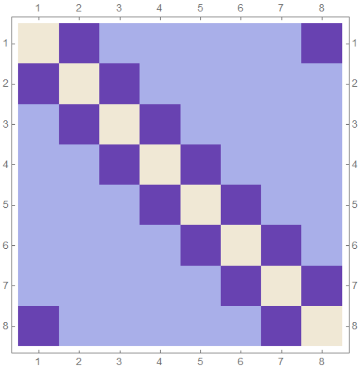
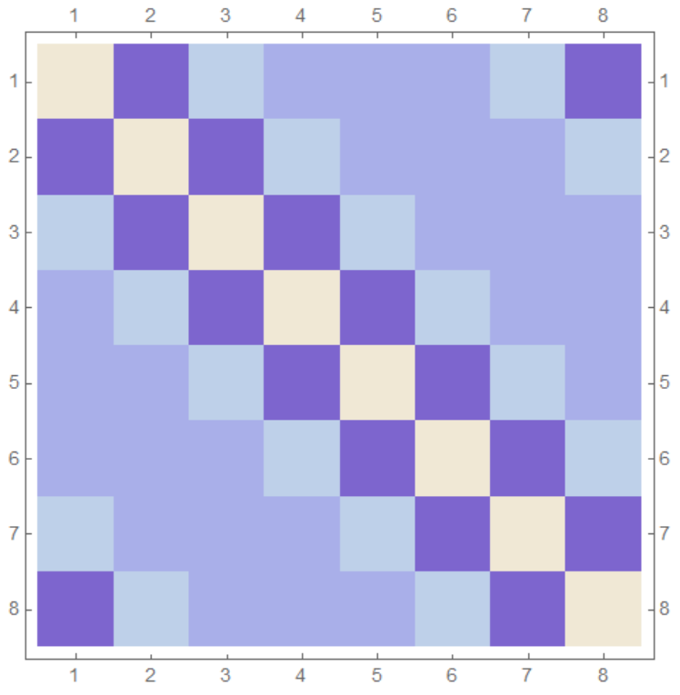
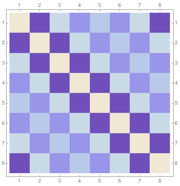
Figure 15: Visual representations of Eqs. (60)-(78). From left to right, the finite-difference, $\delta_{\bar{\phi}}^{2}$-improved, and exact field conjugate-momentum operators obtained from PBCs show increasing non-locality in field space.

Twisted BCs are used for the calculations performed in this work, For the $n_{Q}=3$ system, as defined in Eq. (16). with momentum eigenvalues $k={\pi\over\delta_{\bar{\phi}}}\left(-{7\over 8},-{5\over 8},-{3\over 8},-{1\over 8},{1\over 8},{3\over 8},{5\over 8},{7\over 8}\right)$, the finite-difference, $\delta_{\bar{\phi}}^{2}$-corrected, and the exact conjugate-momentum operators in field space are

$$\tilde{\Pi}^{2}_{\rm finite-difference}=\frac{1}{\delta_{\bar{\phi}}^{2}}\left(\begin{array}[]{cccccccc}2&-1&0&0&0&0&0&1\\ -1&2&-1&0&0&0&0&0\\ 0&-1&2&-1&0&0&0&0\\ 0&0&-1&2&-1&0&0&0\\ 0&0&0&-1&2&-1&0&0\\ 0&0&0&0&-1&2&-1&0\\ 0&0&0&0&0&-1&2&-1\\ 1&0&0&0&0&0&-1&2\\ \end{array}\right)\ \ \ ,$$ (87)

$$\tilde{\Pi}^{2}_{\delta_{\bar{\phi}}^{2}-\rm{improved}}=\frac{1}{\delta_{\bar{\phi}}^{2}}\left(\begin{array}[]{cccccccc}2.5&-1.3&0.083&0&0&0&-0.083&1.3\\ -1.3&2.5&-1.3&0.083&0&0&0&-0.083\\ 0.083&-1.3&2.5&-1.3&0.083&0&0&0\\ 0&0.083&-1.3&2.5&-1.3&0.083&0&0\\ 0&0&0.083&-1.3&2.5&-1.3&0.083&0\\ 0&0&0&0.083&-1.3&2.5&-1.3&0.083\\ -0.083&0&0&0&0.083&-1.3&2.5&-1.3\\ 1.3&-0.083&0&0&0&0.083&-1.3&2.5\\ \end{array}\right)\ \ \ ,$$ (96)

$$\bar{\Pi}^{2}_{\rm exact}=\frac{1}{\delta_{\bar{\phi}}^{2}}\left(\begin{array}[]{cccccccc}3.24&-1.95&0.436&-0.138&0&0.138&-0.436&1.95\\ -1.95&3.24&-1.95&0.436&-0.138&0&0.138&-0.436\\ 0.436&-1.95&3.24&-1.95&0.436&-0.138&0&0.138\\ -0.138&0.436&-1.95&3.24&-1.95&0.436&-0.138&0\\ 0&-0.138&0.436&-1.95&3.24&-1.95&0.436&-0.138\\ 0.138&0&-0.138&0.436&-1.95&3.24&-1.95&0.436\\ -0.436&0.138&0&-0.138&0.436&-1.95&3.24&-1.95\\ 1.95&-0.436&0.138&0&-0.138&0.436&-1.95&3.24\\ \end{array}\right)\ \ .$$ (105)

The corresponding “heat maps” of the entries in each of the twisted operators are shown in Fig. 16.

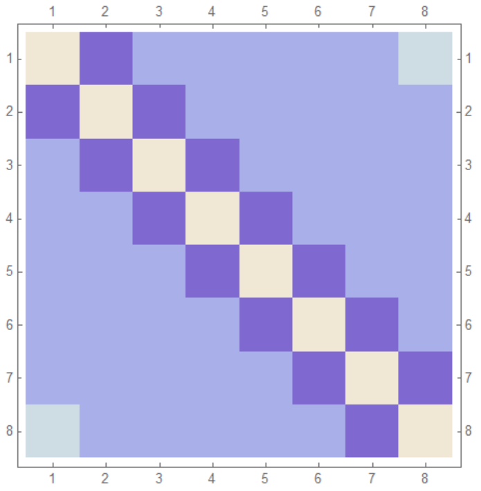
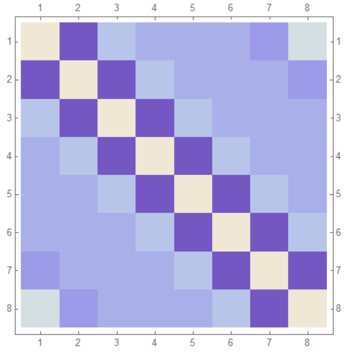
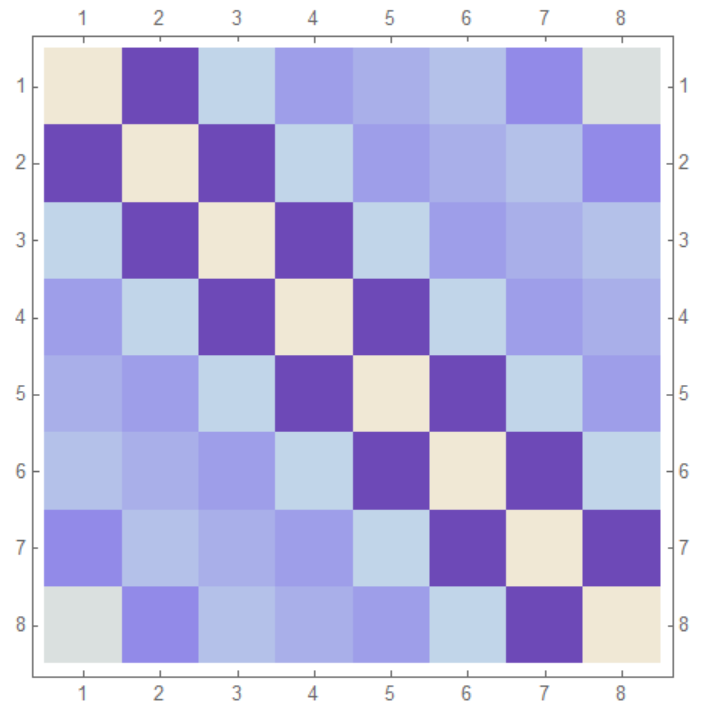
Figure 16: Visual representations of Eqs. (87)-(105). From left to right, the finite-difference, $\delta_{\bar{\phi}}^{2}$-improved, and exact field conjugate-momentum operators obtained from twisted boundary conditions show increasing non-locality in field space.

Appendix F Basic Circuit Construction

In the art and science of quantum circuit development, improvements to generic circuits can often be found when considering the structure of the problem of interest. The techniques presented in this Appendix are well known and exist in standard literature e.g., Ref. Nielsen and Chuang (2011). Because the intended audience of this paper is diverse and a number of considerations for the digitization of the scalar field are made with the following circuit construction in mind, it will be useful to explicitly describe the basic methods for applying unitary operators of the form $e^{i\theta\sigma^{j}\otimes\sigma^{k}\otimes\cdots}$ on NISQ-era quantum hardware capable of implementing $z$-axis rotations $e^{i\theta\sigma^{z}}$. For the Trotterized time evolution of a Pauli-decomposed Hamiltonian, there are two degrees of freedom needed to modify this operation: increasing the number of qubits in the exponentiated tensor product of Paulis and changing the $z$-axis rotation to $x$- or $y$-axis rotations. In order to increase the number of qubits in the tensor product, a string of CNOT operators on either side of a single-qubit rotation may be applied. This computes (and subsequently un-computes) the parity of the of the qubit register down into the last qubit.

$$e^{i\theta\ \sigma^{z}\otimes\sigma^{z}\otimes\sigma^{z}\otimes\sigma^{z}}=\begin{gathered}\Qcircuit@R0.7em@C0.7em{&\ctrl{1}&\qw&\qw&\qw&\qw&\qw&\ctrl{1}&\qw\\ &\targ&\ctrl{1}&\qw&\qw&\qw&\ctrl{1}&\targ&\qw\\ &\qw&\targ&\ctrl{1}&\qw&\ctrl{1}&\targ&\qw&\qw\\ &\qw&\qw&\targ&\gate{e^{i\theta\sigma^{z}}}&\targ&\qw&\qw&\qw}\end{gathered}$$ (110)

To change the axis of rotation for any qubit, the following unitary transformations may be used:

$$\begin{gathered}\Qcircuit@R0.7em@C0.7em{&\gate{X}&\qw}\end{gathered}=\begin{gathered}\Qcircuit@R0.7em@C0.7em{&\gate{H}&\gate{Z}&\gate{H}&\qw}\end{gathered}\qquad\begin{gathered}\Qcircuit@R0.7em@C0.7em{&\gate{Y}&\qw}\end{gathered}=\begin{gathered}\Qcircuit@R0.7em@C0.7em{&\gate{S^{\dagger}}&\gate{H}&\gate{Z}&\gate{H}&\gate{S}&\qw}\end{gathered}$$ (115)

Because applying these transformations in the exponential is equivalent to applying them to the unitary operator itself, these basis-change operations can be implemented as multiplicative unitaries.

$$e^{i\theta\sigma^{x}}=\begin{gathered}\Qcircuit@R0.7em@C0.7em{&\gate{H}&\gate{e^{i\theta\sigma^{z}}}&\gate{H}&\qw}\end{gathered}\qquad e^{i\theta\sigma^{y}}=\begin{gathered}\Qcircuit@R0.7em@C0.7em{&\gate{S^{\dagger}}&\gate{H}&\gate{e^{i\theta\sigma^{z}}}&\gate{H}&\gate{S}&\qw}\end{gathered}$$ (118)

Combining these two degrees of freedom, the exponent of any tensor product of Pauli operators can be created from the single-qubit $z$-axis rotation through use of a CNOT-distributed parity calculation and a change of Pauli bases at the beginning and end of the circuit.

$$e^{i\theta\ \sigma^{x}\otimes\sigma^{y}\otimes\sigma^{x}\otimes\sigma^{z}\otimes\sigma^{y}}=\begin{gathered}\Qcircuit@R0.7em@C0.7em{&\qw&\gate{H}&\ctrl{1}&\qw&\qw&\qw&\qw&\qw&\qw&\qw&\ctrl{1}&\gate{H}&\qw&\qw\\ &\gate{S^{\dagger}}&\gate{H}&\targ&\ctrl{1}&\qw&\qw&\qw&\qw&\qw&\ctrl{1}&\targ&\gate{H}&\gate{S}&\qw\\ &\qw&\gate{H}&\qw&\targ&\ctrl{1}&\qw&\qw&\qw&\ctrl{1}&\targ&\qw&\gate{H}&\qw&\qw\\ &\qw&\qw&\qw&\qw&\targ&\ctrl{1}&\qw&\ctrl{1}&\targ&\qw&\qw&\qw&\qw&\qw\\ &\gate{S^{\dagger}}&\gate{H}&\qw&\qw&\qw&\targ&\gate{e^{i\theta\sigma^{z}}}&\targ&\qw&\qw&\qw&\gate{H}&\gate{S}&\qw}\end{gathered}$$ (124)

Before considering cancellations that usually occur when sequentially implementing operators for Trotterization in this way Hastings et al. (2015), these basic circuits lead to a CNOT contribution of $2(k-1)$ for the implementation of each unitary with a $k$-body Pauli operator in the exponent. This is the counting used for the resource estimates shown in Tables 1, 2, and 3.

Appendix G Lowest-Lying Energy Eigenvalues

The ground state and $1^{st}$ excited state energies of the systems studied in this work are given in Table 4.

System	GS	$1^{st}$
$0+1\ \ \lambda=0\ \ m=1$	${1\over 2}$	${3\over 2}$
$0+1\ \ \lambda=32\ m=1$	0.859 742 690 445 509 019 355 96	2.949 363 767 009 968 902 29
$0+1\ \ \lambda=1\ \ \mu=2$	-22.596 382 373 935 095 119 775 874	-22.596 382 373 935 095 118 634 895
$0+1\ \ \lambda=1\ \ \mu=5$	-933.966 134 532 634 985 047 797 739	-933.966 134 532 634 985 047 797 739
$1+1\ \ \lambda=32\ m=1$	2.124 233 123 438 790 185 081 206 39	4.141 788 964 874 434 527 967 370 80

Table 4: Values of the ground-state and $1^{st}$-excited-state energies for the 1-site and 2-site systems studied in this work. The eigenvalues of the 1-site theory with $\lambda=0$ and $m=1$ (HO) are known exactly. All other ground state values are displayed with a number of digits sufficient to produce the tuning and precision plots that appear in the main text.

Appendix H Noisy Simulations

In this Appendix, we show that in a simple model of quantum noise (step (3) of Fig. 1) representative of near-term quantum hardware, and using first-order Trotterized time evolution (step (2) of Fig. 1), simulation errors exceed the theoretical systematic errors of digitization (step (1) of Fig. 1). This identifies the simulation errors (steps 2,3) as the dominant source of uncertainty. This focuses future improvements on bolstering the system against simulation errors to have the greatest impact on the exploration of scalar fields on near-term quantum devices.

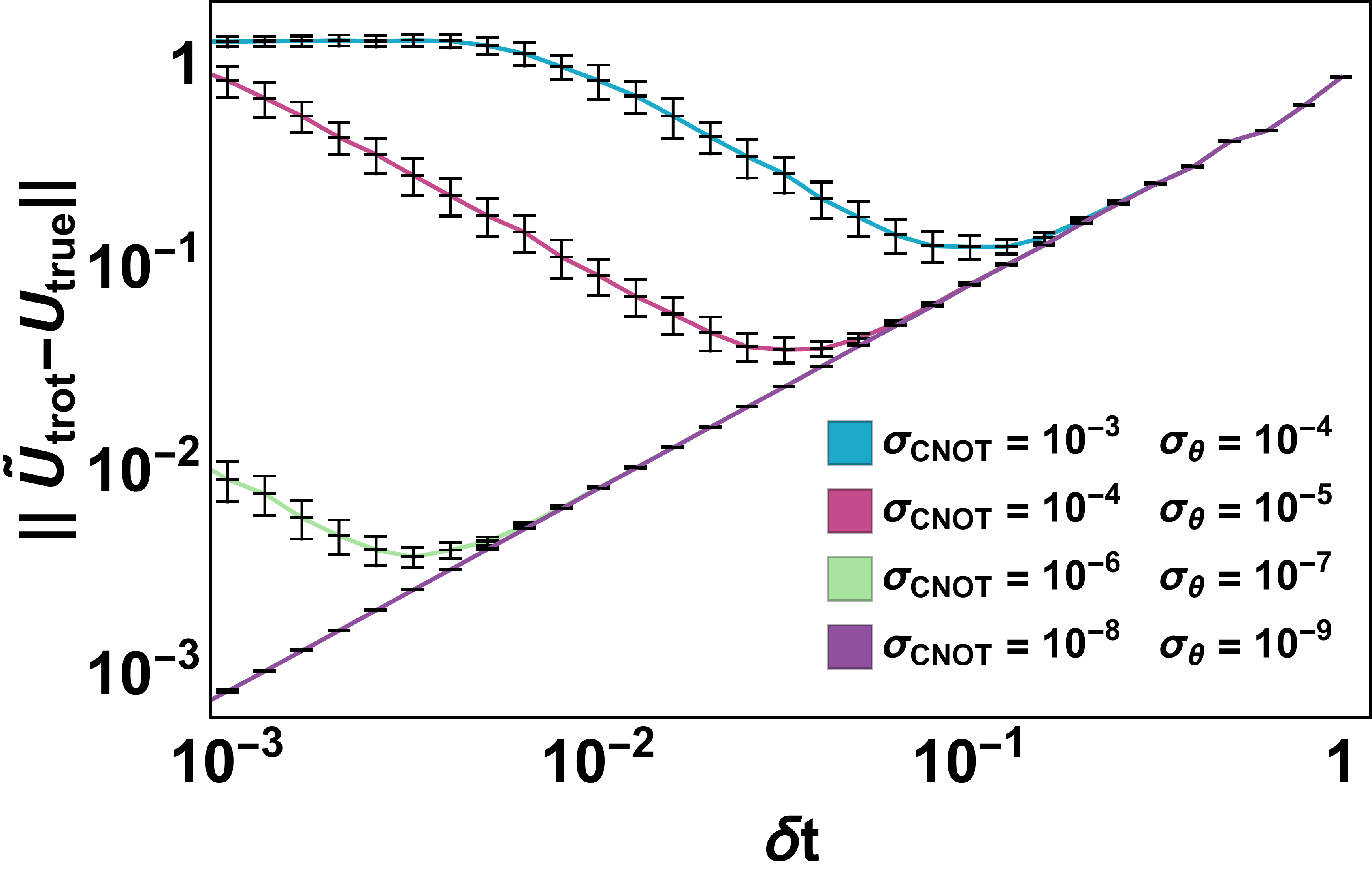
Figure 17: Distance measure (Schatten 1-norm) between the noisily-Trotterized and exactly-digitized time evolution operator (after step (3) and (1) of Fig. 1, respectively) as a function of the Trotter step size, $\delta t$, for an integrated evolution time of $T_{f}=1$. The noisy, first-order Trotterized propagator, $\tilde{U}_{\rm trot}$ is implemented with sampled error rates on 1- and 2- qubit gates set by $\sigma_{\theta}$ and $\sigma_{\rm CNOT}$, respectively. The digitization scheme is defined by $n_{Q}=3$ and $\bar{\phi}_{\rm max}=3.0$. From right-to-left, the calculations deviate from the from the ideal result in the top-to-bottom order of the legend with the last calculation at $\sigma_{\rm CNOT}=10^{-8}$ maintaining visual agreement for the entire plotted domain.

The first quantity to examine in assessing the error landscape specific to the scalar field is the Schatten 1-norm of the time evolution operator evolved to final time $T_{f}=1$ as shown in Fig. 17. The system studied in this and the following figures is the one-site, free scalar field digitized onto three qubits (the minimum number identified in the main text necessary to achieve $\sim 1\%$ errors on the low-energy eigenvalues). Referencing Fig. 2, the tuning of the JLP basis that places the calculation at the NS saturation point and thus optimizes the balance between field-space and momentum-space representations of the wavefunction may be chosen leading to a field-space truncation of $\bar{\phi}_{\rm max}=3.0$. In Fig. 17, $U_{\rm true}$ is the exact, eight-dimensional, digitized propagator described in the qubit system after step (1) in Fig. 1. The Schatten 1-norm of this propagator with the Trotterized propagator $U_{\rm trot}$ (after step (2) in Fig. 1) scales linearly with the Trotter step size, $\delta t$, and is degenerate in this figure with the minimum-error data defined by $\sigma_{\rm CNOT}=10^{-8}$. The noisy, Trotterized propagator $\tilde{U}_{\rm trot}$ (after step (3) in Fig. 1) deviates from this linear scaling at low values of $\delta t$ where the errors of $T_{f}/\delta t$ noisy Trotter steps have accumulated, effectively smearing the evolution. This type of accumulation of fluctuations in gate implementations may be easily visualized in the single qubit case where the uncertainty in the final quantum state eventually wraps a significant portion of the Bloch sphere’s surface. For long evolution, the accumulation of these errors leads to a constant, $\mathcal{O}(1)$ operator norm (as can be seen at $\delta t\sim 3\times 10^{-3}$ with $\sigma_{\rm CNOT}=10^{-3}$). As the noise model implemented here is unitary, containing no effects of decoherence or amplitude damping modeling quantum decoherence of the qubit hardware, this saturation indicates that the system has surpassed a software coherence time, a limit encountered due to imperfect gates (even if implemented on ideal qubits isolated from their environment). Of course, when the gate error rate is reduced, the software coherence time is increased and a longer circuit (smaller $\delta t$ for a fixed $T_{f}=1$) may be implemented before saturation of the propagator’s Schatten 1-norm with the ideal Trotterized propagator. It is a hardware-specific question for future investigation whether NISQ-era digital quantum simulations will be limited by hardware or software coherence times.

The noise model simulated in this Appendix is that of local, unitary errors correlated with the presence of computational operations. For each $m$-qubit gate, an $SU(2)^{\otimes m}$ operator is applied before and after its application with Euler angles sampled from a normal distribution centered at zero with a standard deviation of $\sigma_{\theta}$ and $\sigma_{\rm CNOT}$ for $m=1$ and $m=2$, respectively. All operators with $m>2$ are decomposed into 1- and 2-qubit gates as demonstrated in the main text before implementing this noise model. While this procedure neglects the possible non-unitary, non-Markovian, non-local quantum fluctuations that may plague the calculations implemented on NISQ-era hardware, examining its effects proves enlightening to the limitations imposed by even this simple form of quantum noise. Note that this formulation includes, and is more general than, the noise model used in the creation of Fig. 3 where Gaussian noise was implemented only on the phases applied in conjugate-momentum space. For the simulations of this Appendix, $\sigma_{\rm CNOT}$ is chosen to be one order of magnitude larger than $\sigma_{\theta}$ to express the dominance of 2-qubit errors anticipated in the NISQ-era. The error shown in Fig. 17 represent the standard deviation of the Schatten 1-norm propagated through sampling of the noisy, Trotterized time evolution operator.

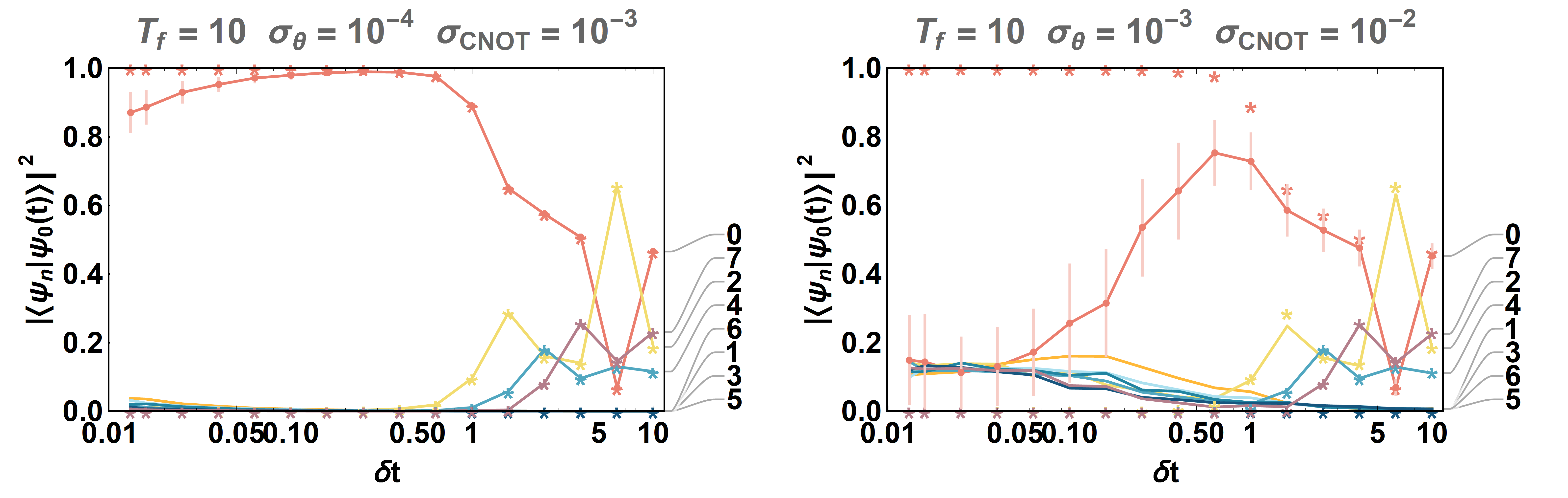
Figure 18: Ground state persistence of a 1-site, free scalar field propagated to time $T_{f}=10$ that has been digitized with $n_{Q}=3$ with $\bar{\phi}_{\rm max}=3.0$ as a function of Trotter step size, $\delta t$, for two error rates. The star-shaped points are calculated from a first-order Trotterized propagator without quantum noise and becomes exact in the limit $\delta t\rightarrow 0$. Points joined by colored lines are sampled with the noise model described in the text at error rates of $\sigma_{CNOT}=10^{-3},10^{-2}$ and $\sigma_{\theta}$ one order of magnitude smaller in each case. Eigenvector indices, $n$, are indicated at the right of each panel.

While the Schatten 1-norm is a succinct distance measure to quantify the effects of Trotterization and successive noisy implementation of the time evolution operator, it remains unclear, beyond perhaps placing loose bounds, how these errors propagate to physical observables likely to be extracted from the quantum calculation. To address quantities of direct relevance to the calculation results, two additional properties are examined: the ground state persistence and the evolution of the expectation value of the field $\langle\phi\rangle(t)$. Figure 18 shows the decomposition of the time evolved ground state across the t = 0 eigenbasis after a total evolution time of $T_{f}=10$ as a function of the Trotter step size, $\delta t$. The star-shaped points are noiseless Trotterizations of the digitized propagator (after step (2) in Fig. 1) and show that the ground state persists for sufficiently small $\delta t$ as $U_{\rm trot}$ becomes exact. When $\delta t$ is sufficiently large, the ground-state persistence diminishes due to errors that are polynomial in $\delta t$ affecting both the energies and eigenvalues of the Trotterized propagator. Moving through step (3) of Fig. 1, the joined points indicate that the ground state persistence falls also at small $\delta t$ where, as was the case with the Schatten 1-norm, noise in the propagator has accumulated. The left panel in Fig. 18 is calculated with $\sigma_{\rm CNOT}=10^{-3}$ while the right panel is calculated with larger fluctuations in the gate errors, $\sigma_{\rm CNOT}=10^{-2}$. The notable difference in the ground-state persistence between these error rates (both being relevant to NISQ-era hardware) is that the former is capable, for specific but existing choice of $\delta t$, of retaining the ground state content at the 1% level while the latter is not capable of achieving this for any choice of $\delta t$. Note that matrix elements to eigenstates 1, 3, 5, and 6 are not excited in the Trotterization and remain of negligible excitation in the noisy Trotterization. This feature dramatically limits the Hilbert-space mixing available to the noisy evolution by effectively decoupling half of the Hilbert space. Even with this structural advantage, the persistence of low-energy eigenstates is seen to be a significant obstacle at noise levels expected in the NISQ-era.

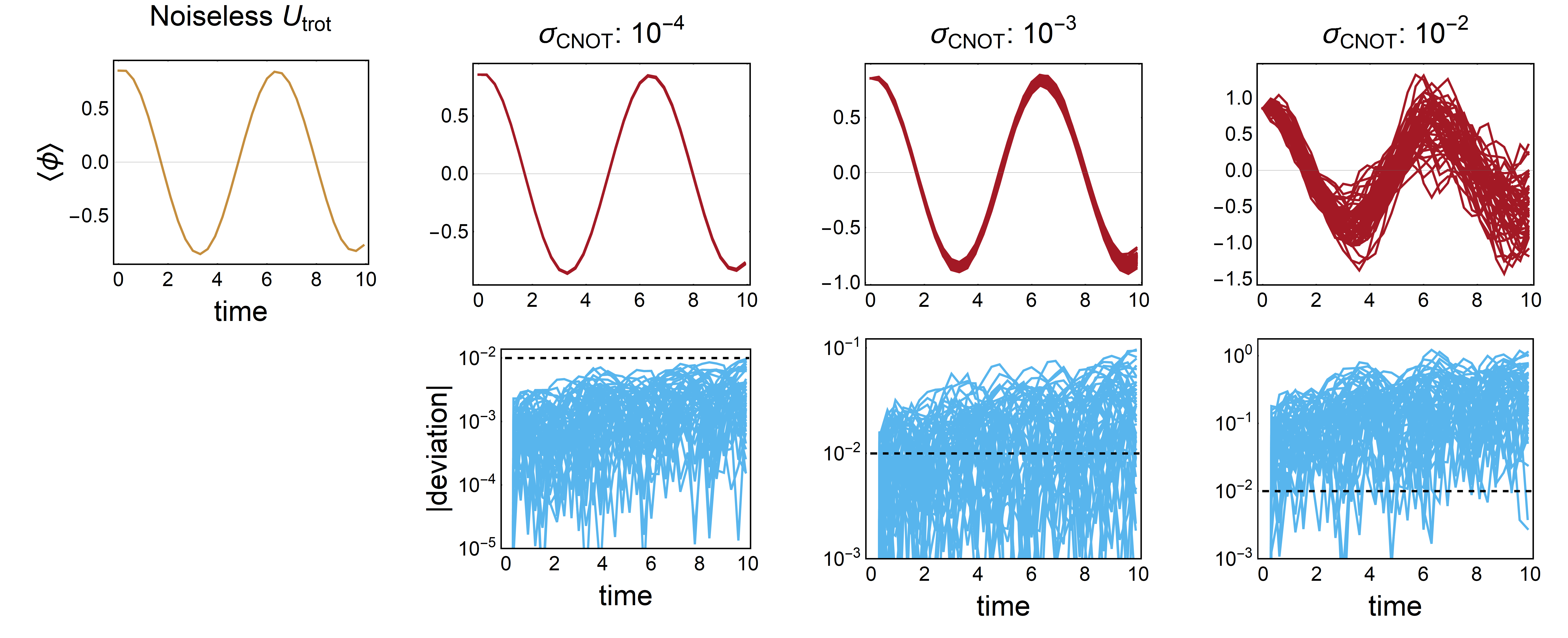
Figure 19: The time evolution of the expectation value of the field operator for a state initialized to the ground state rotated by a single site in $\phi$-space. The evolution in the upper left (gold curve) is the noiseless first-order Trotterization (after step (2) in Fig. 1) with $\delta t=0.3$. The gate-error rate $\sigma_{\rm CNOT}$ increases to the right with $\sigma_{\theta}$ an order of magnitude smaller in each case. The deviation shown in the second row is with respect to the noiseless Trotterization and represents only the errors arising from step (3) of Fig. 1.

For studying the time dependence of the expectation value of the field, $\langle\phi\rangle(t)$, we choose to initialize the system in a state $|\psi_{i}\rangle$ that is the ground state of the system rotated by one site in $\phi$-space. In this state, the expectation value of the field is $\langle\phi\rangle=0.8567$, a value dictated dominantly by the $\phi$-space lattice spacing $\delta_{\phi}=\frac{2\bar{\phi}_{\rm max}}{2^{n_{Q}}-1}=\frac{6}{7}$, with deviations due to the effects of the periodic boundary conditions. This state is in the low-energy sector of the Hilbert space, with the projections $|\langle\psi_{n}|\psi_{i}\rangle|^{2}$ into the lowest three eigenstates, $n=0,1,2$, of 69%, 25%, and 5%. Consequently, this evolution is particularly sensitive to the mixing of low-energy eigenstates. The inaccuracies in the time evolution of $\langle\phi\rangle$ for the highest error rate of $\sigma_{\rm CNOT}=10^{-2}$ are substantial, as can be seen in the right-hand column of Fig. 19. To isolate the noise in this observable (step (3) of Fig. 1), the deviation (light blue curves) between the full noisy expectation value (dark red curves) and that calculated from the noiseless Trotterized propagator (upper left panel, gold curve) is shown in the second row, with gate errors increasing to the right. Figure 19 indicates that the errors stemming from step (3) alone result in $\mathcal{O}(1)$ deviations for this observable with $\sigma_{\rm CNOT}=10^{-3}$. It is only when the error rate is decreased to $\sigma_{\rm CNOT}=10^{-4}$ and $\sigma_{\theta}=10^{-5}$ that $\langle\phi\rangle$ can be determined with $\sim 10^{-2}$ precision with respect to the ideal Trotterization, as emphasized by the black dashed reference line in the second row of Fig. 19. This level of precision is presently unavailable on NISQ-era hardware, indicating that non-negligible error mitigation is required for extracting observables in even small space-time volumes on quantum devices. This situation is expected to persist for an extended period.

We conclude that the digitization errors depicted in step (1) of Fig. 1 can be made a subdominant error source for NISQ-era applications through the tuning procedures described in the main text. The remaining simulation errors of the noisy implementation of a Trotterized time-evolution operator depicted in steps (2, 3) of Fig. 1 are found, under reasonable assumptions, to be significant barriers to implementing even the smallest representation of scalar field theory. While higher-order Trotterizations that would reduce the error in step (2) are known, the implementation of these improved temporal digitizations can require a significantly increased number of quantum gates, necessarily increasing the error in step (3) of Fig. 1. The results of this Appendix emphasize that further study is needed in the directions of algorithmic improvements and error mitigation strategies before the errors of steps (2,3) can be systematically controlled in the same way as in the main text of this paper for the digitization step (1).

It is important to remember that desired precision of a calculation need not be achieved with a single set of simulation parameters ($\delta t$, $\sigma_{\theta,\rm CNOT}$, etc.). While properties of a single parameter set were analysed here, it is also possible (and likely essential in the NISQ-era) to implement a collection of biased or lower-precision calculations and extrapolate to the unbiased or “zero-error” limit. Such an extrapolation in the regime of two-qubit gate errors has been shown to be vital to digitally calculate e.g., the deuteron binding energy Dumitrescu et al. (2018) and the dynamics of pair production in the Schwinger model Klco et al. (2018). In this way, it is possible to achieve precision in an observable beyond the noise levels of available quantum hardware. A thorough investigation for designing collections of quantum simulations ranging in computational expense allowing extrapolations of the effects of noise in NISQ-era devices is now, in the context of controllable digitization errors, a leading avenue for future algorithmic progress towards implementation of scalar fields on NISQ-era quantum devices. Of course, such a program of planning the distributions of resources is not unique to quantum computation, and has been essential in optimizing scientific productivity in high-performance (classical) computing projects, such as the lattice QCD production campaigns in high-energy and nuclear physics.