The [C II]  emission as a molecular gas mass tracer in galaxies at low and high redshift

Abstract

We present ALMA Band 9 observations of the [C II]158$\mu$m emission for a sample of 10 main-sequence galaxies at redshift $z$$\sim$2, with typical stellar masses ($\log$ M_⋆/M${}_{\odot}\sim$10.0–10.9) and star formation rates ($\sim$35–115 M_⊙ yr^-1). Given the strong and well understood evolution of the interstellar medium from the present to $z=2$, we investigate the behaviour of the [C II] emission and empirically identify its primary driver. We detect [C II] from six galaxies (four secure, two tentative) and estimate ensemble averages including non detections. The [C II]-to-infrared luminosity ratio ($L_{\rm[C~{}{\small II}]}$/$L_{\rm IR}$) of our sample is similar to that of local main-sequence galaxies ($\sim 2\times 10^{-3}$), and $\sim$ 10 times higher than that of starbursts. The [C II] emission has an average spatial extent of 4 – 7 kpc, consistent with the optical size. Complementing our sample with literature data, we find that the [C II]  luminosity correlates with galaxies’ molecular gas mass, with a mean absolute deviation of 0.2 dex and without evident systematics: the [C II]-to-H₂ conversion factor ($\alpha_{\rm[C~{}{\small II}]}\sim 30$ M_⊙/L_⊙) is largely independent of galaxies’ depletion time, metallicity, and redshift. [C II]  seems therefore a convenient tracer to estimate galaxies’ molecular gas content regardless of their starburst or main-sequence nature, and extending to metal-poor galaxies at low- and high-redshifts. The dearth of [C II] emission reported for $z>6$–7 galaxies might suggest either a high star formation efficiency or a small fraction of UV light from star formation reprocessed by dust.

1 Introduction

A tight correlation between the star formation rates (SFR) and stellar masses (M_⋆) in galaxies seems to be in place both in the local Universe and at high redshift (at least up to redshift $z\sim 7$, e.g. Bouwens et al. 2012, Steinhardt et al. 2014, Salmon et al. 2015): the so-called “main-sequence” (MS; e.g. Noeske et al. 2007, Elbaz et al. 2007, Daddi et al. 2007, Stark et al. 2009, followed by many others). The normalization of this relation increases with redshift. At fixed stellar mass ($\sim 10^{10}$ M_⊙), $z\sim 1$ galaxies have SFRs comparable to local Luminous Infrared Galaxies (LIRGs); at $z\sim 2$ their SFR is further enhanced and they form stars at rates comparable to local Ultra Luminous Infrared Galaxies (ULIRGs). However, the smooth dynamical disk structure of high-redshift main-sequence sources, together with the tightness of the SFR – M_⋆ relation, disfavour the hypothesis that the intense star formation activity of these galaxies is triggered by major mergers, as by contrast happens at $z=0$ for ULIRGs (e.g., Armus et al. 1987, Sanders & Mirabel 1996, Bushouse et al. 2002). The high SFRs in the distant Universe seem instead to be sustained by secular processes (e.g. cold gas inflows) producing more stable star formation histories (e.g., Noeske et al. 2007, Davé et al. 2012).

Main sequence galaxies are responsible for $\sim 90$% of the cosmic star formation rate density (e.g. Rodighiero et al. 2011, Sargent et al. 2012), whereas the remaining $\sim$ 10% of the cosmic SFR density is due to sources strongly deviating from the main sequence, showing enhanced SFRs and extreme infrared luminosities. Similarly to local ULIRGs, star formation in these starburst (SB) galaxies is thought to be ignited by major merger episodes (e.g., Elbaz et al. 2011, Nordon et al. 2012, Hung et al. 2013, Schreiber et al. 2015, Puglisi et al. 2017). Throughout this paper we will consider as starbursts all the sources that fall $>4$ times above the main sequence (Rodighiero et al., 2011).

To understand the mechanisms triggering star formation, it is crucial to know the molecular gas reservoir in galaxies, which forms the main fuel for star formation (e.g. Bigiel et al. 2008), at the peak of the cosmic star formation history ($z\sim 2$). Due to their high luminosities, the starbursts have been the main sources studied for a long time, although they only represent a small fraction of the population of star-forming galaxies. Only recently it has been possible to gather large samples of $z\sim$ 1 – 2 main-sequence sources and investigate their gas content thanks to their CO and dust emission (e.g. Genzel et al. 2010, Carilli & Walter 2013, Tacconi et al. 2013, Combes et al. 2013, Scoville et al. 2015, Daddi et al. 2015, Walter et al. 2016, Dunlop et al. 2017). Observing the CO transitions at higher redshift, however, becomes challenging since the line luminosity dims with cosmological distance, the contrast against the CMB becomes lower (e.g. da Cunha et al. 2013), and it weakens as metallicity decreases (as expected at high $z$). Some authors describe the latter effect stating that a large fraction of molecular gas becomes “CO dark”, meaning that the CO line no longer traces H₂ (e.g. Wolfire et al. 2010, Shi et al. 2016, Madden et al. 2016, Amorín et al. 2016, Glover & Smith 2016) and therefore the CO luminosity per unit gas mass is much lower on average for these galaxies. Similarly, the dust content of galaxies decreases with metallicity and therefore it might not be a suitable tracer of molecular gas at high redshift. An alternative possibility is to use other rest-frame far-infrared (IR) lines instead. Recently [C I]  has been proposed as molecular gas tracer (e.g., Papadopoulos & Greve 2004, Walter et al. 2011, Bothwell et al. 2016, Popping et al. 2017), although it is fainter than many CO transitions and this is still an open field of research. Alternatively the [C II]  ${}^{2}P_{3/2}$ – ${}^{2}P_{1/2}$ transition at 158 $\mu$m might be a promising tool to investigate the gas physical conditions in the distant Universe (e.g. Carilli & Walter 2013).

[C II]  has been identified as one of the brightest fine structure lines emitted from star-forming galaxies. It has a lower ionization potential than H I  (11.3 eV instead of 13.6 eV) and therefore it can be produced in cold atomic interstellar medium (ISM), molecular, and ionized gas. However, several studies have argued that the bulk of galaxies’ [C II]  emission originates in the external layers of molecular clouds heated by the far-UV radiation emitted from hot stars with $\gtrsim$ 60 – 95% of the total [C II]  luminosity arising from photodissociation regions (PDRs, e.g. Stacey et al. 1991, Sargsyan et al. 2012, Rigopoulou et al. 2014, Cormier et al. 2015, Diaz-Santos et al. 2017, Croxall et al. 2017). In particular, Pineda et al. (2013) and Velusamy & Langer (2014) showed that $\sim$ 75% of the [C II]  emission in the Milky Way is coming from the molecular gas; this is in good agreement with simulations showing that 60% – 85% of the [C II]  luminosity emerges from the molecular phase (Olsen et al. 2017, Accurso et al. 2017b, Vallini et al. 2015). There are also observational and theoretical models suggesting that [C II]  is a good tracer of the putative “CO dark” gas. The main reason for this is the fact that in the outer regions of molecular clouds, where the bulk of the gas-phase carbon resides, H₂ is shielded either by dust or self-shielded from UV photodissociation, whereas CO is more easily photodissociated into C and C⁺. This H₂ is therefore not traced by CO, but it mainly emits in [C II]  (e.g. Maloney & Black 1988, Stacey et al. 1991, Madden et al. 1993, Poglitsch et al. 1995, Wolfire et al. 2010, Pineda et al. 2013, Nordon & Sternberg 2016, Fahrion et al. 2017, Glover & Smith 2016). Another advantage of using the [C II]  emission line is the fact that it possibly traces also molecular gas with moderate density. In fact, the critical density needed to excite the [C II]  emitting level through electron impacts is $>$ 10 particle/cc ($\sim$ 5 - 50 cm^-3). For comparison, the critical density needed for CO excitation is higher ($\sim$ 1000 H/cc), so low-density molecular gas can emit [C II], but not CO (e.g. Goldsmith et al. 2012, Narayanan & Krumholz 2017). This could be an important contribution given the fact that $\sim$ 30% of the molecular gas in high-redshift galaxies has a density $<$ 50 H/cc (Bournaud et al. in prep., 2017), although detailed simulations of the [C II]  emission in turbulent disks are still missing and observational constraints are currently lacking.

The link between the [C II]  emission and star-forming regions is further highlighted by the well known relation between the [C II]  and IR luminosities ($L_{\mathrm{[C~{}{\small II}]}}$ and $L_{\mathrm{IR}}$ respectively, e.g. De Looze et al. 2010, De Looze et al. 2014, Popping et al. 2014, Herrera-Camus et al. 2015, Popping et al. 2016, Olsen et al. 2016, Vallini et al. 2016), since the IR luminosity is considered a good indicator of the SFR (Kennicutt, 1998). However, this relation is not unique and different galaxies show distinct $L_{\mathrm{[C~{}{\small II}]}}/L_{\mathrm{IR}}$ ratios. In fact,

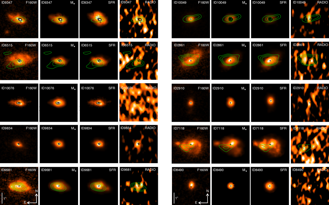
Figure 1: HST and ALMA observations of our sample galaxies. For each source we show the HST/WFC3 image taken with the F160W filter, the stellar mass map, the star formation rate map, and the radio observations taken with VLA. The overplotted black contours, when present, show the $>3\sigma$ [C II]  emission. The green contours indicate the $>3\sigma$ 850 $\mu$m continuum. The color scale in all panels is linear and it is chosen to show galaxies’ features at best. The units of the color bars are the following: counts s^-1 for F160W, 10⁹ M_⊙ for the stellar mass maps, M_⊙ yr^-1 for the SFR maps, and Jy for the radio.

in the local Universe main-sequence sources show a constant $\langle L_{\mathrm{[C~{}{\small II}]}}/L_{\mathrm{IR}}\rangle\sim$ 0.002 – 0.004, although with substantial scatter (e.g., Stacey et al. 1991, Malhotra et al. 2001, Stacey et al. 2010; Cormier et al. 2015, Smith et al. 2017, Diaz-Santos et al. 2017). Whereas when including also local starburst galaxies (LIRGs and ULIRGs) with $L_{\mathrm{IR}}>10^{11}$ L_⊙, the [C II]$/$IR luminosity ratio drops significantly by up to an order of magnitude (e.g. Malhotra et al. 1997, Stacey et al. 2010, Díaz-Santos et al. 2013, Farrah et al. 2013, Magdis et al. 2014). These sources are usually referred to as “[C II]  deficient” with respect to main-sequence galaxies. It has been shown that not only the [C II]  emission drops, but also other far-IR lines tracing both PDRs and H II  regions (e.g. [O I]145 $\mu$m, [N II]122 $\mu$m, [O III]88 $\mu$m, [O I]63 $\mu$m, [N III]57 $\mu$m, Graciá-Carpio et al. 2011, Zhao et al. 2013, Diaz-Santos et al. 2017) show a deficit when starbursts are considered. This is likely related to the enhanced star formation efficiency (SFE = SFR/$M_{\mathrm{mol}}$) of starbursts with respect to local main-sequence galaxies, consistent with the results by Daddi et al. (2010) and Genzel et al. (2010). This relation between the $L_{\mathrm{[C~{}{\small II}]}}/L_{\mathrm{IR}}$ and galaxies’ SFE could be due to the fact that the average properties of the interstellar medium in main-sequence and starburst sources are significantly different: the highly compressed and more efficient star formation in starburst could enhance the ionization parameters and drive to lower line to continuum ratios (Graciá-Carpio et al., 2011). At high redshift, observations become more challenging, mainly due to the fainter fluxes of the targets: so far $z>1$ studies have mainly targeted IR selected sources (e.g., the most luminous sub-millimeter galaxies and quasars), whereas measurements for IR fainter main-sequence targets are still limited (e.g., Stacey et al. 2010, Hailey-Dunsheath et al. 2010, Ivison et al. 2010, Swinbank et al. 2012, Riechers et al. 2014, Magdis et al. 2014, Huynh et al. 2014, Brisbin et al. 2015). Therefore it is not clear yet if high-$z$ main-sequence galaxies, which have similar SFRs as (U)LIRGs, are expected to be [C II]  deficient. With our sample we start to push the limit of current observations up to redshift $z\sim 2$.

The goal of this paper is to understand whether main-sequence, $z\sim 2$ galaxies are [C II]  deficient and investigate what are the main physical parameters the [C II]  emission line is sensitive to. Interestingly we find that its luminosity traces galaxies’ molecular gas mass and could therefore be used as an alternative to other proxies (e.g. CO, [CI], or dust emission). Given its brightness and the fact that it remains luminous at low metallicities where the CO largely fades, this emission line might become a valuable resource to explore the galaxies’ gas content at very high redshift. Hence understanding the [C II]  behaviour in $z\sim 2$ main-sequence galaxies, whose physical properties are nowadays relatively well constrained, will lay the ground for future explorations of the ISM at higher redshift.

The paper is structured as follows: in Section 2 we present our observations, sample selection, and data analysis; in Section 3 we discuss our results; in Section 4 we conclude and summarize. Throughout the paper we use a flat $\Lambda$CDM cosmology with $\Omega_{\mathrm{m}}=0.3$, $\Omega_{\mathrm{\Lambda}}=0.7$, and $H_{0}=70\,\mathrm{km\,s^{-1}Mpc^{-1}}$. We assumed a Chabrier (2003) initial mass function (IMF) and, when necessary, we accordingly converted literature results obtained with different IMFs.

2 Observations and data analysis

In this Section we discuss how we selected the sample and we present our ALMA observations together with available ancillary data. We also report the procedure we used to estimate the [C II]  and continuum flux of our sources. Finally, we describe the literature data that we used to complement our observations, for which full details are given in Appendix.

2.1 Sample selection and ancillary data

To study the ISM properties of high-redshift main-sequence galaxies, we selected targets in the GOODS-S field (Giavalisco et al. 2004, Nonino et al. 2009), which benefits from extensive multi-wavelength coverage.

Our sample galaxies were selected on the basis of the following criteria: 1) having spectroscopic redshift in the range $1.73<z<1.94$ to target the [C II]  emission line in ALMA Band 9. We made sure that the selected galaxies would have been observed in a frequency region of Band 9 with good atmospheric transmission. Also, to minimize overheads, we selected our sample so that multiple targets could be observed with the same ALMA frequency setup; 2) being detected in the available Herschel data; 3) having SFRs and M_⋆ typical of main-sequence galaxies at this redshift, as defined by Rodighiero et al. (2014, they all have sSFR/sSFR${}_{\mathrm{MS}}<$ 1.7); 4) having undisturbed morphologies, with no clear indications of ongoing mergers, as inferred from the visual inspection of HST images. Although some of the optical images of these galaxies might look disturbed, their stellar mass maps are in general smooth (Figure 1), indicating that the irregularities visible in the imaging are likely due to star-forming clumps rather than major mergers (see, e.g., Cibinel et al. 2015).

Our sample therefore consists of 10 typical star-forming, main-sequence galaxies at redshift $1.73\leq z\leq 1.94$. Given the high ionization lines present in its optical spectrum, one of them (ID10049) appears to host an active galactic nucleus (AGN). This source was not detected in [C II]  and retaining it or not in our final sample does not impact the implications of this work.

Deep Hubble Space Telescope (HST) observations at optical (HST/ACS F435W, F606W, F775W, F814W, and F850LP filters) and near-IR (HST/WFC3 F105W, F125W, and F160W filters) wavelengths are available from the CANDELS survey (Koekemoer et al. 2011, Grogin et al. 2011). Spitzer and Herschel mid-IR and far-IR photometry in the wavelength range 24 $\mu$m – 500 $\mu$m is also available (Elbaz et al. 2011, Wang et al. in prep. 2017). Finally, radio observations at $\sim$ 5 cm (6 GHz) were taken with the Karl G. Jansky Very Large Array (VLA) with 0.3” $\times$ 0.6” resolution (Rujopakarn et al., 2016).

Thanks to these multiwavelength data, we created resolved stellar mass and SFR maps for our targets, following the method described by Cibinel et al. (2015). In brief, we performed pixel-by-pixel spectral energy distribution (SED) fitting considering all the available HST filters mentioned above, after having convolved all the images with the PSF of the matched $H_{\mathrm{F160W}}$ band, useful also to increase the signal-to-noise (S/N). We considered Bruzual & Charlot (2003)

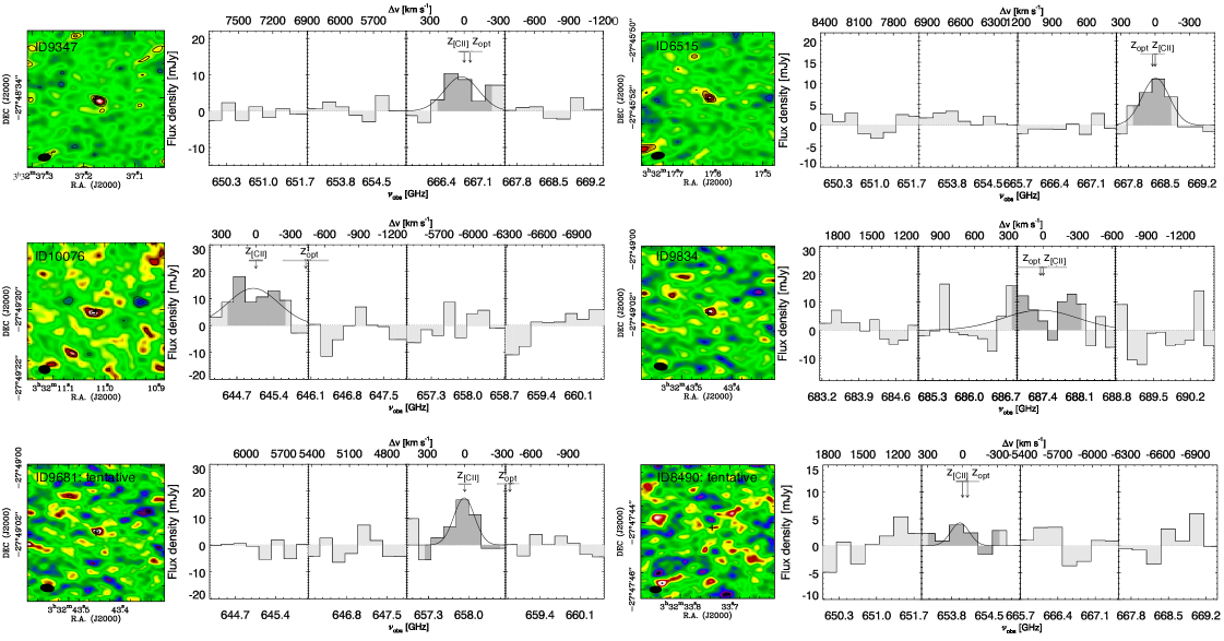
Figure 2: ALMA spectra of the [C II]  detections of our sample. Left panels: ALMA 2D maps of the [C II]  emission line. The black solid and dashed contours indicate respectively the positive and negative 3$\sigma$, 4$\sigma$, and 5$\sigma$ levels. The beam is reported as the black filled ellipse. Each stamp has a size of 4” $\times$ 4”. The black cross indicates the galaxy center, as estimated from the HST F160W imaging. Some tapering has been done for illustrative purposes, although we used the untapered maps for the analysis. Right panels: 1D spectra of the [C II]  detected sources extracted using a PSF to maximize the S/N (notice that in this figure we did not scale the fluxes of the spectra extracted with PSF to match those obtained when using an exponential function with larger size as reported in Table 2). The dark grey shaded areas indicate the 1-$\sigma$ velocity range over which the flux has been measured. The frequencies corresponding to the optical and [C II]  redshifts are marked with arrows. The horizontal bars indicate the 1$\sigma$ uncertainty associated to the optical (light gray) and [C II]  (dark gray) redshift estimate. For illustrative purposes we also report the Gaussian fit of the emission lines: it was not used to estimate the line fluxes, but only as an alternative estimate of the galaxies’ redshift (Section 2.3).

templates with constant SFR to limit the degeneracy with dust extinction. We corrected the fluxes for dust extinction following the prescriptions by Calzetti et al. (2000). The stellar population age in the models varied between 100 Myr and 2 Gyr, assuming fixed solar metallicity. In Figure 1 we show the resulting SFR and stellar mass maps, together with the HST $H_{\mathrm{F160W}}$-band imaging. The stellar mass computed summing up all the pixels of our maps is in good agreement with that estimated by Santini et al. (2014) fitting the global ultraviolet (UV) to IR SED (they differ $<$ 30% with no systematic trends). In the following we use the stellar masses obtained from the global galaxies’ SED, but our conclusions would not change considering the estimate from the stellar mass maps instead.

Spectroscopic redshifts for our sources are all publicly available and were determined in different ways: 5 of them are from the GMASS survey (Kurk et al., 2013), one from the K20 survey (Cimatti et al. 2002, Mignoli et al. 2005), 2 were determined by Popesso et al. (2009) from VLT/VIMOS spectra, one was estimated from our rest-frame UV Keck/LRIS spectroscopy as detailed below, and one had a spectroscopic redshift estimate determined by Pope et al. (2008) from PAH features in the Spitzer/IRS spectrum. With the exception of three sources, all the redshifts were estimated from rest-frame UV absorption lines. This is a notoriously difficult endeavour especially when, given the faint UV magnitudes of the sources, the signal-to-noise ratio (S/N) of the UV continuum is moderate, as for our targets. We note that having accurate spectroscopic redshifts is crucial for data like that presented here: ALMA observations are carried out using four, sometimes adjacent, sidebands (SBs) covering 1.875 GHz each, corresponding to only 800 km s^-1 rest-frame in Band 9 (or equivalently $\Delta z=0.008$). This implies that the [C II]  emission line might be outside the covered frequency range for targets with inaccurate spectroscopic redshift. In general we used at least two adjacent SBs (and up to all 4 in one favourable case) targeting, when possible, galaxies at comparable redshifts (Table 1).

Given the required accuracy in the redshift estimate, before the finalization of the observational setups, we carefully re-analyzed all the spectra of our targets to check and possibly refine the redshifts already reported in the literature. To this purpose, we applied to our VLT/FORS2 and Keck UV rest-frame spectra the same approach described in Gobat et al. (2017b, although both the templates we used and the wavelength range of our data are different). Briefly, we modelled the $\sim$ 4000 – 7000 Å  range of the spectra using standard Lyman break galaxy templates from Shapley et al. (2003), convolved with a Gaussian to match the resolution of our observations. The redshifts were often revised with respect to those published with variations up to $\sim$ a few $\times 10^{-3}$. Our new values, reported in Table 2, match those measured in the independent work of Tang et al. (2014) and have formal uncertainties $\lesssim 1$–2$\times 10^{-3}$ ($\lesssim$ 100$-200~{}$km s^-1), corresponding to an accuracy in the estimate of the [C II]  observed frequency of $\sim$ 0.25 GHz.

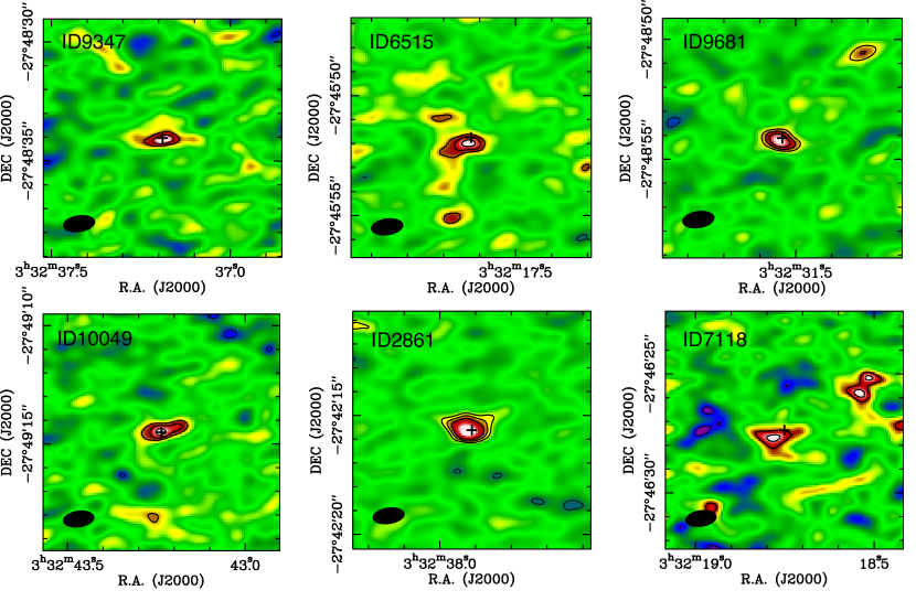
Figure 3: ALMA maps of the continuum detections at 850 $\mu$m. The black contours indicate the 3$\sigma$, 4$\sigma$, and 5$\sigma$ levels. The beam is reported as the black filled ellipse. Each stamp has a size of 10” $\times$ 10”. The black cross indicated the galaxy center, as estimated from the HST imaging. Some tapering has been done for illustrative purposes, although we used the untapered maps for the analysis.

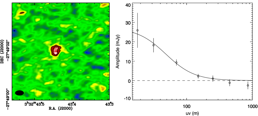
Figure 4: Stacking of the four secure [C II]  detections of our sample. Left panel: image obtained aligning the four galaxies at their HST peak positions and stacking their visibilities. From 3$\sigma$ and 4$\sigma$ contours are shown. Right panel: signal amplitude as a function of the uv distance (namely the baseline length). We fitted the data with an exponential model (black curve). A similar fit is obtained when fitting the data with a gaussian model with FWHM $\sim$ 0.6”.

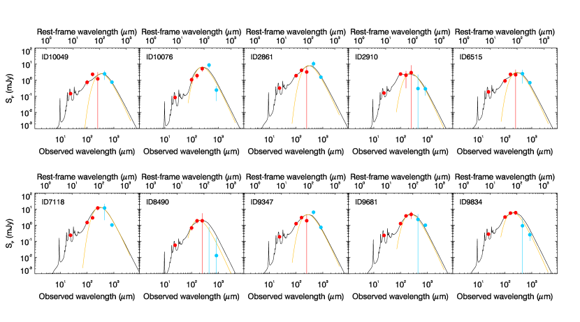
Figure 5: Spectral energy distribution fits for our sample galaxies. Herschel and Spitzer measurements are reported as red filled circles and the ALMA ones as cyan filled circles. The black curve is the best model fit and the yellow line indicates the best modified black body fit.

2.2 Details of ALMA observations

We carried out ALMA Band 9 observations for our sample during Cycle 1 (PI: E. Daddi, Project ID: 2012.1.00775.S) with the goal of detecting the [C II]  emission line at rest-frame 158 $\mu$m ($\nu_{\mathrm{rest-frame}}=1900.54$ GHz) and the underlying continuum, redshifted in the frequency range $\nu_{\mathrm{obs}}=645$ – $696$ GHz. Currently this is the largest sample of galaxies observed with ALMA at this redshift with available [C II]  measurements given the difficulty to carry out such observations in Band 9. We observed each galaxy, depending on its IR luminosity, for 8 – 13 minutes including overheads to reach a homogeneous sensitivity of 1.5 – 2 mJy/beam over a bandwidth of 350 km s^-1. We set a spectral resolution of 0.976 MHz (0.45 km s^-1 – later binning the data to substantially lower velocity resolutions) and we requested observations with a spatial resolution of about 1” (configuration C32-1) to get integrated flux measurements of our sources. However, the observations were taken in the C32-3 configuration with a synthesized beam FWHM $=$ 0.3” $\times$ 0.2” and a maximum recoverable scale of $\sim$ 3.5”. Our sources were therefore resolved. To check if we could still correctly estimate total [C II]  fluxes, we simulated with CASA (McMullin et al., 2007) observations in the C32-3 configuration of extended sources with sizes comparable to those of our galaxies, as detailed in Appendix A. We concluded that, when fitting the sources in the uv plane, we could measure their correct total fluxes, but with substantial losses in terms of effective depth of the data. Figure 12 in Appendix A shows how the total flux error of a source increases, with respect to the case of unresolved observations, as a function of its size expressed in units of the PSF FWHM (see also Equation 7 that quantifies the trend). Given that our targets are 3 – 4 times larger than the PSF, we obtained a flux measurement error 5 – 10 times higher than expected, hence correspondingly lower S/N ratios. The depth of our data, taken with 0.2” resolution, is therefore equivalent to only 10 – 30s of integration if taken with 1^′′ resolution. However, when preparing the observations we considered conservative estimates of the [C II]  flux and therefore several targets were detected despite the higher effective noise.

As part of the same ALMA program, besides the Band 9 data, we also requested additional observations in Band 7 to detect the 850 $\mu$m continuum, which is important to estimate dust masses for our targets (see Section 2.4). For each galaxy we reached a sensitivity of 140 $\mu$Jy/beam on the continuum, with an integration time of $\sim 2$ minutes on source. The synthesised beam has FWHM $=$ 1” $\times$ 0.5” and the maximum recoverable scale is $\sim$ 6”.

We note that there is an astrometry offset between our ALMA observations and the HST data released in the GOODS-S field (Appendix B). Although it is negligible in right ascension ($\Delta RA=0.06$”), it is instead significant in declination ($\Delta DEC=-0.2$”, $>3\sigma$ significant), in agreement with estimates reported by other studies (e.g. Dunlop et al. 2017, Rujopakarn et al. 2016, Barro et al. 2016, Aravena et al. 2016b, Cibinel et al. 2017). We accounted for this offset when interpreting our data by shifting the HST coordinate system to match that of ALMA. In Figure 1 we show the astrometry-corrected HST stamps. However, in Table 2 we report the uncorrected HST coordinates to allow an easier comparison with previous studies. The ALMA target positions are consistent with those from VLA.

2.3 [C II]  emission line measurements

The data were reduced with the standard ALMA pipeline based on the CASA software (McMullin et al., 2007). The calibrated data cubes were then converted to uvfits format and analyzed with the software GILDAS (Guilloteau & Lucas, 2000).

To create the velocity-integrated [C II]  line maps for our sample galaxies it was necessary to determine the spectral range over which to integrate the spectra. This in turn requires a 1D spectrum, that needs to be extracted at some spatial position and with a source surface brightness distribution model (PSF or extended). We carried out the following iterative procedure, similar to what described in Daddi et al. (2015 and in preparation) and Coogan et al. (2018).

We fitted, in the uv plane, a given source model (PSF, but also Gaussian and exponential profiles, tailored to the HST size of the galaxies) to all four sidebands and channel per channel, with fixed spatial position determined from the astrometry-corrected HST images. We looked for positive emission line signal in the resulting spectra. When a signal was present, we averaged the data over the channels maximizing the detection S/N and we fitted the resulting single channel dataset to obtain the best fitting line spatial position. If this was different from the spatial position of the initial extraction we proceeded to a new spectral extraction at the new position, and iterate the procedure until convergence was reached.

2.3.1 Individual [C II]  detections

Four galaxies converged to secure detections (Figure  2): they have emission line significance $>5\sigma$ in the optimal channel range. The detections are robust against the model used for the extraction of the 1D spectra: the frequency range used for the lines’ identification would not change if we extracted the 1D spectra with a Gaussian or exponential model instead of a PSF. The optimizing spatial positions for spectral extractions were consistent with the HST peak positions, typically within the PSF FWHM (Figure  2), and the spectra extracted with Gaussian or exponential models were in any case invariant with respect to such small spatial adjustments.

We estimated the redshift of the four detections in two ways, both giving consistent results (redshift differences $<0.001$) and similar formal redshift uncertainties: 1) we computed the signal-weighted average frequency within the line channels, and 2) we fitted the 1D spectrum with a Gaussian function. Following Coogan et al. (2018) simulations of a similar line detection procedure, and given the S/N of these detections, we concluded that redshift uncertainties estimated in this way are reliable. We compared our redshift estimates for these sources with those provided by our VLT and Keck data analysis, and in the literature (Section 2). They generally agree, with no significant systematic difference and a median absolute deviation (MAD) of 200 km s^-1 (MAD${}_{\rm z}=0.002$). This accuracy is fully within the expected uncertainties of both our optical and [C II] redshift (see Table 2), thus increasing the reliability of the detections considering that the line search was carried out over a total $\Delta z=0.035$.

Given the fact that our sources are extended, we estimated their total [C II]  flux by fitting their average emission line maps in the uv plane with exponential models (whereas by using a PSF model instead we would have underestimated the fluxes). We used the following procedure. Our sample is composed of disk-like galaxies as shown in Figure 1. Although in some cases (e.g. ID7118) some clumps of star formation are visible both in the HST imaging and in the spatially resolved SFR maps, the resolved stellar mass maps are smooth, as expected for unperturbed sources, and mainly show the diffuse disk seen also in our ALMA observations. We therefore determined the size of the galaxy disks by fitting the stellar mass maps with an exponential profile (Freeman, 1970), using the GALFIT algorithm (Peng et al., 2010). We checked that there were not structured residuals when subtracting the best-fit model from the stellar mass maps. We then extracted the [C II]  flux by fitting the ALMA data in the $uv$ plane, using the Fourier Transform of the 2D exponential model, with the GILDAS task uv_fit. We fixed the size and center of the model on the basis of the effective radius and peak coordinates derived from the optical images, corrected for the astrometric offset determined as in Appendix B. As a result, we obtained the total [C II]  flux of our sources. Given the larger uncertainties associated to extended source models with respect to the PSF case (Appendix B), this procedure returns $>3\sigma$ total flux measurements for the four sources (even if original detections were $>5\sigma$). We checked that fluxes and uncertainties determined with the uvmodelfit task provided by CASA would give consistent results. We also checked the robustness of our flux measurements against the assumed functional form of the model: fitting the data with a Gaussian profile instead of an exponential would give consistent [C II]  fluxes. Finally, we verified that the uncertainties associated to the flux measurement in each channel are consistent with the channel to channel fluctuations, after accounting for the continuum emission and excluding emission lines.

Table 1: Log of the observations

ID	Date	$z_{\mathrm{SB1}}$	$z_{\mathrm{SB2}}$	$z_{\mathrm{SB3}}$	$z_{\mathrm{SB4}}$	texp	Noise R.M.S.
						(min)	(mJy/beam)
(1)	(2)	(3)	(4)	(5)	(6)	(7)	(8)
9347	03 Nov 2013	1.8388 – 1.8468	1.8468 – 1.8548	1.9014 – 1.9098	1.9158 – 1.9242	17.14	16.83
6515	03 Nov 2013	1.8388 – 1.8468	1.8468 – 1.8548	1.9014 – 1.9098	1.9158 – 1.9242	17.14	15.76
10076	04 Nov 2013	1.8771 – 1.8852	1.8852 – 1.8935	1.9332 – 1.9418	1.9418 – 1.9503	10.58	21.69
9834	04 Nov 2013	1.7518 – 1.7593	1.7593 – 1.7668	1.7668 – 1.7744	1.7744 – 1.7820	11.09	15.39
9681	04 Nov 2013	1.8771 – 1.8852	1.8852 – 1.8935	1.9332 – 1.9418	1.9418 – 1.9503	10.58	18.72
10049	03 Nov 2013	1.8388 – 1.8468	1.8468 – 1.8548	1.9014 – 1.9098	1.9158 – 1.9242	15.12	11.60
2861	04 Nov 2013	1.7213 – 1.7291	1.7291 – 1.7364	1.8024 – 1.8102	1.8102 – 1.8180	9.58	30.10
2910	04 Nov 2013	1.7518 – 1.7593	1.7593 – 1.7668	1.7668 – 1.7744	1.7744 – 1.7820	11.09	14.36
7118	04 Nov 2013	1.7213 – 1.7291	1.7291 – 1.7364	1.8024 – 1.8102	1.8102 – 1.8180	9.58	51.00
8490	03 Nov 2013	1.8388 – 1.8468	1.8468 – 1.8548	1.9014 – 1.9098	1.9158 – 1.9242	16.13	15.44

Columns (1) Galaxy ID; (2) Date of observations; (3) Redshift range covered by the ALMA sideband #1; (4) Redshift range covered by the ALMA sideband #2; (5) Redshift range covered by the ALMA sideband #3; (6) Redshift range covered by the ALMA sideband #4. For the sources highlighted in bold all the four sidebands are contiguous; (7) Integration time on source; (8) Noise r. m. s.

However, the returned fluxes critically depend on the model size that we used and that we determined from the optical images. If we were to use a smaller (larger) size, the inferred flux would be correspondingly lower (higher). Unfortunately, the size of the emission cannot be constrained from the data on individual sources, given the limited S/N ratio. There have been claims that sizes estimated from optical data could be larger than those derived from IR observations (Díaz-Santos et al. 2013, Psychogyios et al. 2016). This could possibly bias our analysis and in particular our flux estimates to higher values. As a check, we aligned our [C II]  detections at the HST positions and stacked them (coadding all visibilities) to increase the S/N (Figure 4). In the uv space the overall significance of the stacked detection is $\sim 10\sigma$. The probability that the signal is not resolved (i.e., a point source, which would have constant amplitude versus uv distance) is $<10^{-5}$. We then fitted the stacked data with an exponential profile, leaving its size free to vary during the fit. We get an exponential scale length for the [C II]  emission of $0.65\pm 0.15^{\prime\prime}$ (corresponding to $\sim$ 4 – 7 kpc), corrected for the small broadening that could affect the stack due to the uncertainties in the determination of the sources’ exact position, and with a significance of S/N(size) $\sim 4\sigma$. The reported size uncertainty was estimated by GILDAS in the fit and the modelling of the signal amplitude versus uv range signal shows that it is reliable (Figure 4). This indicates that on average the optical sizes that we used in the analysis are appropriate for the fit of our ALMA data and that these four galaxies are indeed quite extended (the average optical size of the 4 galaxies is $\sim$ 0.7^′′, $2\sigma$, in good agreement with what measured in the [C II] stack).

We also used the stack of our four detected sources to further check our [C II] flux estimates. We compared the flux measured by fitting the stacking with that obtained by averaging the fluxes of individual detections. As mentioned above, the flux of the stacking critically depends on the adopted model size, but in any case the measurement was highly significant (S/N$>5$) even when leaving the size free to vary during the fit. When fitting the stack with a model having an exponential scale length $\sim 0.6$” we obtained estimates consistent with the average flux of individual sources.

2.3.2 Tentative and non detections

In our sample, six sources were not individually detected by the procedure discussed in the previous section. In these cases we searched for the presence of weaker [C II] signal in the data by evaluating the recovered signal when eliminating all degrees of freedom in the line search, namely measuring at fixed HST position, using exponential models with the fixed optical size for each galaxy and conservatively averaging the signal over a large velocity range tailored to the optical redshifts. In particular, we created emission line maps by averaging channels over 719 km s^-1, around the frequency corresponding to the optical redshift. This velocity width is obtained by summing in quadrature 3 times the MAD redshift accuracy (obtained considering optical and [C II] redshifts, as discussed above for the four detections) and the average FWHM of the detected emission lines. We find weak signal from two galaxies at S/N$>2.3$ (ID9681 and ID8490, see Table 2) and no significant signal from the others. Given that with this approach there are no degrees of freedom, the probability of obtaining each tentative detection (namely the probability of having a $>2.3\sigma$ signal) is Gaussian and equal to $\sim$ 0.01. Furthermore, when considering the six sources discussed above, we expect to find $<0.1$ false detections. We therefore conclude that the $2.3\sigma$ signal found for our two tentative detections is real.

For the four sources with no detected signal we considered $3\sigma$ flux upper limits, as estimated from emission line maps integrated over a 719 km s^-1 bandwidth. There are different possible reasons why these galaxies do not show any signal. Two of them (ID7118 and ID2861) have substantially worse data quality, probably due to the weather stability and atmosphere transparency during the observations, with about 3 times higher noise than the rest of the sample. Their $L_{\mathrm{[C~{}{\small II}]}}/L_{\mathrm{IR}}$ upper limits are not very stringent and are substantially higher than the rest of the sample (Table 2). Possible reasons for the other two non detections (ID2910 and ID10049) are the following. (i) These sources might be more extended than the others, and therefore their signal might be further suppressed. However this is unlikely, as their optical size is smaller than the average one of the detected sources (Table 3). (ii) They might have fainter IR luminosity than the other sample galaxies. The $L_{\mathrm{IR}}$ that we used to predict the [C II]  luminosity for these two undetected sources was overestimated before the observations. However, using the current $L_{\mathrm{IR}}$ values (Section 2.4), we obtain $L_{\mathrm{[C~{}{\small II}]}}/L_{\mathrm{IR}}$ upper limits comparable with the ratios estimated for the detected sources. (iii) A wrong optical redshift estimate can also explain the lack of signal from one of these undetected galaxies: ID10049 is an AGN with broad lines, and the determination of its systemic redshift obtained considering narrow line components ($z=1.920$) is possibly more uncertain than the redshift range covered by our ALMA observations ($z=1.9014$–1.9098 and $z=1.9158$–1.9242; Table 1; for comparison, the original literature redshift was 1.906). For ID2910 instead the optical spectrum seems to yield a solid redshift and the covered redshift range is the largest (Table 1), so the [C II] line should have been observed. This source probably has fainter [C II]  luminosity than the others (i.e. lower $L_{\mathrm{[C~{}{\small II}]}}/L_{\mathrm{IR}}$).

Finally, we stacked the four [C II]  non-detections in the $uv$ plane and fitted the data with an exponential profile, with size fixed to the average optical size of the sources entering the stacking. This still did not yield a detection. Since two non-detections have shallower data than the others and at least one might have wrong optical redshift, in the rest of the analysis we do not consider the average [C II]  flux obtained from the stacking of these sources.

The coordinates, sizes, [C II]  fluxes, and luminosities of our sample galaxies are presented in Table 2. We subtracted from the [C II]  fluxes the contribution of the underlying 158 $\mu$m rest-frame continuum as measured in our ALMA Band 9 data (Section 2.4). For galaxies with no detected continuum at 450 $\mu$m (see Section 2.4), we computed the predicted 158 $\mu$m rest-frame continuum flux from the best-fit IR SEDs and reduced the [C II]  fluxes accordingly.

2.3.3 Average [C II] signal

We have previously stacked the four detections to measure their average size, compare it with the optical one, and understand if we were reliably estimating the fluxes of our sources (Section 2.3.1). Now we want to estimate the average [C II]  signal of our sample to investigate its mean behaviour. We therefore add to the previous stack also the two tentative detections and one non-detected source. We report in the following the method that we used to stack these galaxies and the reasons why we excluded from the stack three non-detected sources.

We aligned the detections and tentative detections and stacked them coadding all visibilities. We also coadded the non-detected galaxy ID2910, but we do not include the other three sources for reasons outlined above. . We fitted the resulting map with an exponential model with size fixed to the average optical size of the sources entering the stacking. We finally subtracted the contribution of the rest-frame 158 $\mu$m continuum by decreasing the estimated flux by 10% (namely the average continuum correction applied to the sources of our sample, see Section 2.4). We obtained a $\sim 10\sigma$ detection that we report in Table 2.

Table 2: Measurements for our sample galaxies

ID	RA	DEC	$z_{\mathrm{opt}}$	$z_{\mathrm{[C~{}{\small II}]}}$	$F_{\mathrm{450\mu m}}$	$F_{\mathrm{850\mu m}}$	$F_{\mathrm{[C~{}{\small II}]}}$	$L_{\mathrm{[C~{}{\small II}]}}$	log($L_{\mathrm{IR}}$)	$L_{\mathrm{[C~{}{\small II}]}}/L_{\mathrm{IR}}$	$\Delta v$
	[deg]	[deg]			[mJy]	[mJy]	[mJy]	[109 L⊙]	[log(L⊙)]	[$10^{-3}$]	[km s-1]
(1)	(2)	(3)	(4)	(5)	(6)	(7)	(8)	(9)	(10)	(11)	(12)
9347	53.154900	-27.809397	1.8503 $\pm$ 0.0010	1.8505 $\pm$ 0.0002	$<$ 8.85	0.75 $\pm$ 0.24	21.28 $\pm$ 6.73	0.95 $\pm$ 0.30	11.80 $\pm$ 0.05	$1.51^{+0.51}_{-0.50}$	534.3
6515	53.073375	-27.764353	1.8440 $\pm$ 0.0010	1.8438 $\pm$ 0.0002	$<$5.76	0.71 $\pm$ 0.18	24.50 $\pm$ 6.57	1.23 $\pm$ 0.33	11.68 $\pm$ 0.04	$2.57^{+0.73}_{-0.73}$	365.4
10076	53.045904	-27.822156	1.9418 $\pm$ 0.0020	1.9462 $\pm$ 0.0006	$<$9.69	$<$0.57	29.03 $\pm$ 9.14	2.40 $\pm$ 0.76	11.91 $\pm$ 0.03	$2.95^{+0.96}_{-0.96}$	548.1
9834	53.181029	-27.817147	1.7650 $\pm$ 0.0020	1.7644 $\pm$ 0.0003	$<$4.52	$<$0.45	15.34 $\pm$ 2.21	1.29 $\pm$ 0.19	11.99 $\pm$ 0.02	$1.32^{+0.22}_{-0.22}$	627.3
9681	53.131350	-27.814922	1.8852 $\pm$ 0.0010	–	$<$8.04	1.01 $\pm$ 0.24	17.59 $\pm$ 7.63	1.81 $\pm$ 0.79	11.84 $\pm$ 0.04	$2.62^{+1.17}_{-1.16}$	719.0
10049	53.180149	-27.820603	1.9200a	–	$<$4.32	0.77 $\pm$ 0.16	$<5.65$	$<$0.60	11.60 $\pm$ 0.06	$<$1.51	719.0
2861	53.157905	-27.704283	1.8102 $\pm$ 0.0010	–	$<$15.35	1.56 $\pm$ 0.28	$<$40.11	$<$3.84	12.00 $\pm$ 0.03	$<$3.84	719.0
2910	53.163610	-27.705320	1.7686 $\pm$ 0.0010	–	$<$5.94	$<$0.54	$<$12.73	$<$1.17	11.76 $\pm$ 0.08	$<$2.03	719.0
7118	53.078130	-27.774187	1.7290a	–	$<$16.5	1.05 $\pm$ 0.29	$<$56.16	$<$4.94	12.06 $\pm$ 0.01	$<$4.30	719.0
8490	53.140593	-27.795632	1.9056 $\pm$ 0.0010	–	$<$4.5	$<$0.48	6.80 $\pm$ 2.85	0.71 $\pm$ 0.30	11.54 $\pm$ 0.06	$2.05^{+0.92}_{-0.90}$	719.0
Stackb	–	–	1.8536 $\pm$ 0.004	–	–	–	15.59 $\pm$ 1.79	1.25 $\pm$ 0.14	11.81 $\pm$ 0.05	$1.94^{+0.34}_{-0.32}$	604.6

Columns (1) Galaxy ID; (2) Right ascension; (3) Declination; (4) Redshift obtained from optical spectra; (5) Redshift estimated by fitting the [C II]  emission line (when detected) with a Gaussian in our 1D ALMA spectra. The uncertainty that we report is the formal error obtained from the fit; (6) Observed-frame 450$\mu$m continuum emission flux; (7) Observed-frame 850$\mu$m continuum flux; (8) [C II]  emission line flux. We report upper limits for sources with S/N $<2$; (9) [C II]  emission line luminosity; (10) IR luminosity integrated over the wavelength range 8 – 1000 $\mu$m as estimated from SED fitting (Section 2.4); (11) [C II]-to-bolometric infrared luminosity ratio; (12) Line velocity width.
Notes ^aID10049 is a broad line AGN, its systemic redshift is uncertain and it might be outside the frequency range covered by Band 9. The redshift of ID7118 is based on a single line identified as H$\alpha$. If this is correct the redshift uncertainty is $<0.001$. ^b Stack of the 7 galaxies of our sample with reliable [C II]  measurement (namely, ID9347, ID6515, ID10076, ID9834, ID9681, ID8490, ID2910, see Section 2.3.3 for a detailed discussion). We excluded from the stack ID2861 and ID7118 since the quality of their data is worse than for the other galaxies and their [C II]  upper limits are not stringent. We also excluded ID10049 since it is an AGN and, given that its redshift estimate from optical spectra is highly uncertain, the [C II]  emission might be outside the redshift range covered by our ALMA observations. See Section 2.3.2 for a detailed discussion.

The average $L_{\mathrm{[C~{}{\small II}]}}/L_{\mathrm{IR}}$ ratio obtained from the stacking of the seven targets mentioned above is $(1.94^{+0.34}_{-0.32})\times 10^{-3}$. This is in agreement with that obtained by averaging the individual ratios of the same seven galaxies ($L_{\mathrm{[C~{}{\small II}]}}/L_{\mathrm{IR}}=(1.96^{+0.19}_{-0.10})\times 10^{-3}$) where this ratio was obtained averaging the $L_{\mathrm{[C~{}{\small II}]}}/L_{\mathrm{IR}}$ ratio of the seven targets. In particular, the [C II]  flux of ID2910 is an upper limit and therefore we considered the case of flux equal to 1$\sigma$ (giving the average $L_{\mathrm{[C~{}{\small II}]}}/L_{\mathrm{IR}}$ = $1.96\times 10^{-3}$) and the two extreme cases of flux equal to 0 or flux equal to 3$\sigma$, from where the quoted uncertainties. Through our analysis and in the plots we consider the value $L_{\mathrm{[C~{}{\small II}]}}/L_{\mathrm{IR}}=(1.94^{+0.34}_{-0.32})\times 10^{-3}$.

Table 3: Physical properties of our sample galaxies

ID	SFR	log(M⋆)	log Mdust	log M${}_{\mathrm{mol}}^{\mathrm{SK}}$	log M${}_{\mathrm{mol}}^{\mathrm{dust}}$	log M${}_{\mathrm{mol}}^{\mathrm{[CII]}}$	sSFR/sSFRMS	$\log<$U$>$	Re	Z
	[M⊙ yr-1]	[log(M⊙)]	[log(M⊙)]	[log(M⊙)]	[log(M⊙)]	[log(M⊙)]			[arcsec]
(1)	(2)	(3)	(4)	(5)	(6)	(7)	(8)	(9)	(10)	(11)
9347	62.9${}^{+7.9}_{-7.0}$	10.5	8.5$\pm$0.5	10.70	10.50$\pm$0.57	10.51${}^{+0.13}_{-0.19}$	1.1	1.2$\pm$0.5	1.02	8.6
6515	47.7${}^{+4.3}_{-3.9}$	10.9	8.5$\pm$0.4	10.58	10.40$\pm$0.42	10.62${}^{+0.12}_{-0.16}$	0.4	1.2$\pm$0.4	0.77	8.7
10076	81.6${}^{+6.0}_{-5.6}$	10.3	8.4$\pm$0.2	10.77	10.46$\pm$0.23	10.91${}^{+0.13}_{-0.19}$	1.7	1.4$\pm$0.2	0.76	8.6
9834	98.9${}^{+5.4}_{-5.1}$	10.7	8.2$\pm$0.3	10.84	10.20$\pm$0.16	10.60${}^{+0.10}_{-0.12}$	1.2	1.7$\pm$0.3	0.43	8.7
9681	69.3${}^{+5.9}_{-5.5}$	10.6	8.3$\pm$0.5	10.71	10.29$\pm$0.49	10.78${}^{+0.16}_{-0.27}$	1.0	1.5$\pm$0.5	0.89	8.6
10049	39.7${}^{+5.7}_{5.0}$	10.7	8.7$\pm$0.2	10.52	10.70$\pm$0.29	$<10.37$	0.4	0.8$\pm$0.2	0.29	8.7
2861	101.6${}^{+6.5}_{-6.1}$	10.8	9.0$\pm$0.3	10.85	10.97$\pm$0.30	$<11.13$	1.1	0.9$\pm$0.3	0.99	8.7
2910	57.4${}^{+11.1}_{-9.3}$	10.4	8.1$\pm$0.5	10.64	10.18$\pm$0.55	$<10.59$	1.3	1.5$\pm$0.5	0.58	8.6
7118	114.8${}^{+2.9}_{-2.9}$	10.9	9.1$\pm$0.2	10.89	11.03$\pm$0.22	$<11.21$	1.1	0.9$\pm$0.2	1.13	8.7
8490	34.4${}^{+5.2}_{-4.5}$	10.0	7.8$\pm$0.4	10.46	9.98$\pm$0.45	10.38${}^{+0.16}_{-0.26}$	1.2	1.6$\pm$0.4	0.44	8.5
Stacka	64.6${}^{+7.9}_{-7.0}$	10.6	8.3$\pm$0.1	10.69	10.26$\pm$0.34	10.62${}^{+0.04}_{-0.05}$	1.1	1.4$\pm$0.1	0.70	8.6

Columns (1) Galaxy ID; (2) Star formation rate as calculated from the IR luminosity: $SFR=10^{-10}L_{\mathrm{IR}}$ (Kennicutt, 1998). Only the star-forming component contributing to the IR luminosity was used to estimate the SFR, as contribution from a dusty torus was subtracted; (3) Stellar mass. The typical uncertainty is $\sim$ 0.2 dex; (4) Dust mass; (5) Gas mass estimated from the integrated Schmidt-Kennicutt relation (Sargent et al., 2014, Equation 4). The measured dispersion of the relation is 0.2 dex. Given that the errors associated to the SFR are $<0.1$ dex, for the M${}_{\mathrm{mol}}^{\mathrm{SK}}$ we consider typical uncertainties of 0.2 dex.; (6) Gas mass estimated from the dust mass considering a gas-to-dust conversion factor dependent on metallicity (Magdis et al., 2012); (7) Gas mass estimated from the observed [C II]  luminosity considering a [C II]-to-H₂ conversion factor $\alpha_{\mathrm{[C~{}{\small II}]}}=31$ M_⊙/L_⊙. The uncertainties that we report do not account for the $\alpha_{\rm[C~{}{\small II}]}$ uncertainty and they only reflect the [C II]  luminosity’s uncertainty; (8) Distance from the main sequence as defined by Rodighiero et al. (2014); (9) Average radiation field intensity; (10) Galaxy size as measured from the optical HST images; (11) Gas-phase metallicity $12+\log(\mathrm{O/H})$.
Notes ^a Stack of the 7 galaxies of our sample with reliable [C II]  measurement (namely, ID9347, ID6515, ID10076, ID9834, ID9681, ID8490, ID2910). We excluded from the stack ID2861 and ID7118 since the quality of their data is worse than for the other galaxies and their [C II]  upper limits are not stringent. We also excluded ID10049 since it is an AGN and, given that its redshift estimate from optical spectra is highly incertain, the [C II]  emission might be outside the redshift range covered by our ALMA observations. See Section 2.3.2 for a detailed discussion.

2.4 Continuum emission at observed-frame 450 $\mu$m and 850 $\mu$m

Our ALMA observations cover the continuum at $\sim$ 450 $\mu$m (Band 9 data) and 850 $\mu$m (Band 7 data). We created averaged continuum maps by integrating the full spectral range for the observations at 850 $\mu$m. For the 450 $\mu$m continuum maps instead we made sure to exclude the channels where the flux is dominated by the [C II]  emission line.

We extracted the continuum flux by fitting the data with an exponential profile, adopting the same procedure described in Section 2.3. The results are provided in Table 2, where 3$\sigma$ upper limits are reported in case of non-detection.

The estimated continuum fluxes were used, together with the available Spitzer and Herschel data (Elbaz et al., 2011), to properly sample the IR wavelengths, perform SED fitting, and reliably determine parameters such as the infrared luminosity and the dust mass ($M_{\mathrm{dust}}$). The Spitzer and Herschel data were deblended using prior sources to overcome the blending problems arising from the large PSFs and allow reliable photometry of individual galaxies (Béthermin et al. 2010, Roseboom et al. 2010, Elbaz et al. 2011, Lee et al. 2013, Béthermin et al. 2015, Liu et al. 2017). Following the method presented in Magdis et al. (2012), we fitted the IR photometry with Draine & Li (2007) models, supplemented by the use of a single temperature modified black body (MBB) fit to derive a representative dust temperature of the ISM. In these fits we considered the measured Spitzer, Herschel, and ALMA flux (even if S/N $<$ 3, e.g. there is no detection) along with the corresponding uncertainty instead of adopting upper limits. The contribution of each photometric point to the best fit is weighted by its associated uncertainty. If we were to use upper limits in these fits instead our conclusions would not have changed. The IR SEDs of our targets are shown in Figure 5 and the derived parameters are summarized in Table 3. We note that our method to estimate dust masses is based on the fit of the full far-IR SED of the galaxies, not on scaling a single band luminosity in the Rayleigh-Jeans regime (e.g. as suggested by Scoville et al. 2017). This fact together with the high quality photometry at shorter wavelengths allowed us to properly constrain the fitted parameters also for galaxies with highly uncertain 850 $\mu$m measurements. We also determined the average radiation field intensity as $\langle U\rangle=L_{\mathrm{IR}}/(125M_{\mathrm{dust}})$ (Magdis et al., 2012). Uncertainties on $L_{\mathrm{IR}}$ and $M_{\mathrm{dust}}$ were quantified using Monte Carlo simulations, as described by Magdis et al. (2012).

The IR luminosities we estimated ($L_{\mathrm{IR}}=L[8$–$1000\,\mu$m]) for our sample galaxies lie between $3.5\times 10^{11}$ – $1.2\times 10^{12}$ L_⊙, with a median value of $7.1\times 10^{11}$ L_⊙, and we probe a range of dust masses between $7.0\times 10^{7}$ – $1.2\times 10^{9}$ M_⊙, with a median value of $3.0\times 10^{8}$ M_⊙. Both our median estimate of $L_{\mathrm{IR}}$ and $M_{\mathrm{dust}}$ are in excellent agreement with literature estimates for main-sequence galaxies at similar redshift (e.g. $L_{\mathrm{IR}}=6\times 10^{11}$ L_⊙ and $M_{\mathrm{dust}}=3\times 10^{8}$ M_⊙ at redshift $1.75<z<2.00$ in Béthermin et al. 2015, for a mass selected sample with an average $M_{\star}$ comparable to that of our galaxies). The $\langle U\rangle$ parameters that we determined range between 6 – 45, consistent with the estimates provided by Magdis et al. (2012) and Béthermin et al. (2015) for main-sequence galaxies at a similar redshift.

Finally, we estimated the molecular gas masses of our galaxies with a twofold approach. (1) Given their stellar mass and the mass-metallicity relation by Zahid et al. (2014) we estimated their gas phase metallicity. We then determined the gas-to-dust conversion factor ($\delta_{\mathrm{GDR}}$) for each source, depending on its metallicity, as prescribed by Magdis et al. (2012). And finally we estimated their molecular gas masses as $M_{\mathrm{mol}}=\delta_{\mathrm{GDR}}\times M_{\mathrm{dust}}$, given the dust masses obtained from the SED fitting. (2) Given the galaxies SFRs and the integrated Schmidt-Kennicutt relation for main-sequence sources reported by Sargent et al. (2014), we estimated their molecular gas masses. We estimated the uncertainties taking into account the SFR uncertainties and the dispersion of the Schmidt-Kennicutt relation. By comparing the galaxies detected in the ALMA 850 $\mu$m data that allow us to obtain accurate dust masses, we concluded that both methods give consistent results (see Table 3). In the following we use the $M_{\mathrm{mol}}$ obtained from the Schmit-Kennicutt relation since, given our in-hand data, it is more robust especially for galaxies with no 850 $\mu$m detection. Furthermore, it allows us to get a more consistent comparison with other high-$z$ literature measurements (e.g. the gas masses for the sample of Capak et al. 2015 have been derived using the same Schmidt-Kennicutt relation, as reported in Appendix C).

2.5 Other samples from the literature

To explore a larger parameter space and gain a more comprehensive view, we complemented our observations with multiple [C II]  datasets from the literature, both at low and high redshift (Stacey et al. 1991, Stacey et al. 2010, Gullberg et al. 2015, Capak et al. 2015, Diaz-Santos et al. 2017, Cormier et al. 2015, Brauher et al. 2008, Contursi et al. 2017, Magdis et al. 2014, Huynh et al. 2014, Ferkinhoff et al. 2014, Schaerer et al. 2015, Brisbin et al. 2015, Hughes et al. 2017, Accurso et al. 2017a). In Appendix C we briefly present these additional samples and discuss how the physical parameters that are relevant for our analysis (namely the redshift, [C II], IR, and CO luminosity, molecular gas mass, sSFR, and gas-phase metallicity) have been derived; in Table LABEL:tab:acii we report them.

3 Results and Discussion

The main motivation of this work is to understand which is the dominant physical parameter affecting the [C II] luminosity of galaxies through cosmic time. In the following we investigate whether our $z\sim 2$ sources are [C II]  deficient and if the [C II]-to-IR luminosity ratio depends on galaxies’ distance from the main-sequence. We also investigate whether the [C II]  emission can be used as molecular gas mass tracer for main-sequence and starburst galaxies both at low and high redshift. Finally we discuss the implications of our results on the interpretation and planning of $z\gtrsim 5$ observations.

3.1 The [C II]  deficit

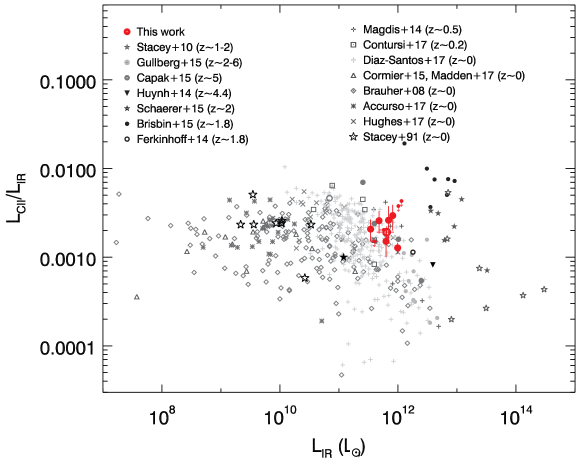
Figure 6: Ratio between the [C II]  and IR (8 – 1000 $\mu$m) luminosity of our sample galaxies, as a function of the IR luminosity. Different symbols indicate distinct datasets: our [C II]  detections (large red filled circles), our [C II]  upper limits for the non-detections (small red filled circles), the average value of our sample (empty red circle), Stacey et al. (2010, grey filled stars indicate star-forming galaxies, grey empty stars indicate AGN or starbursts), Stacey et al. (1991, black empty stars), Gullberg et al. (2015, light grey filled circles), Capak et al. (2015, dark grey filled circles indicate their measurements, dark grey emtpy circles indicate the stack of their non detections), Diaz-Santos et al. (2017, grey crosses), Cormier et al. (2015, black triangles), Brauher et al. (2008, grey diamond), Contursi et al. (2017, grey squares), Magdis et al. (2014, dark grey crosses), Huynh et al. (2014, black downward triangle), Schaerer et al. (2015, black filled star), Brisbin et al. (2015, black filled circles), Ferkinhoff et al. (2014, black empty circle), Hughes et al. (2017, grey crosses), Accurso et al. (2017a, grey asterisks). We note that we are plotting the de-magnified IR luminosity for the sample of lensed galaxies by Gullberg et al. (2015): we considered that the [C II]  emission line is magnified by the same factor as the IR (see discussion in the text and Gullberg et al. 2015). The magnification factors are taken from Spilker et al. (2016). Similarly, the sources by Brisbin et al. (2015) might be lensed, but the magnification factors are unknown and therefore we plot the observed values.

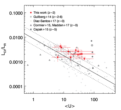
Figure 7: Correlation between the [C II]-to-IR luminosity ratio and the intensity of the radiation field. The symbols are the same as reported in Figure 6 caption, but we only show the samples with available $\langle U\rangle$ measurements (the method used to estimate $\langle U\rangle$ for the various samples is detailed in Section 3.1). The fit of the local sample from Diaz-Santos et al. (2017) is reported (black solid line) together with the standard deviation (black dashed lines).

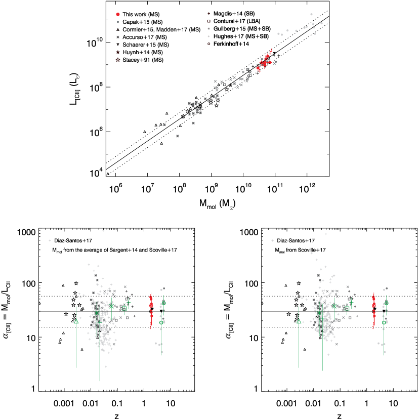
Figure 8: Correlation between the [C II]  luminosity and the molecular gas mass. Top panel: L${}_{\mathrm{[C~{}{\small II}]}}$ – M_mol relation. The symbols are the same as reported in Figure 6 caption, but we only show the samples with available M_mol estimates. In the legend we highlight the nature of the galaxies in each sample (e.g. main-sequence, starburst, Ly break analogs). The fit of the data is reported (black solid line) together with the standard deviation (black dashed lines). Bottom panels: the [C II]-to-H₂ conversion factor ($\alpha_{\mathrm{[C~{}{\small II}]}}$) as a function of redshift. The average $\alpha_{\mathrm{[C~{}{\small II}]}}$ for main-sequence galaxies is reported (black solid line) together with the standard deviation (black dashed lines). The median and median absolute deviation of each sample is plotted (green large symbols). The difference between the left and right panels concerns how the molecular gas mass was estimated for the sample of local galaxies from Diaz-Santos et al. (2017, light gray crosses). Since CO observations for this sample are not available, we estimated $M_{\mathrm{mol}}$, given the sSFR of each source, considering the relation between the depletion time and sSFR of galaxies. In the left panel we report the estimates obtained by averaging the trend reported by Sargent et al. (2014) and Scoville et al. (2017), whereas in the right panel we report the estimates obtained considering the trend by Scoville et al. (2017) only (see Section 3.3 for a more detailed discussion).

In the local Universe, the majority of main-sequence galaxies have [C II]  luminosities that scale linearly with their IR luminosity showing a constant $L_{\mathrm{[C~{}{\small II}]}}/L_{\mathrm{IR}}$ ratio, although substantial scatter is present (e.g., Stacey et al. 1991, Malhotra et al. 2001, Stacey et al. 2010, Cormier et al. 2015, Smith et al. 2017). However, local (U)LIRGs appear to have a different behaviour: they are typically [C II]  deficient with respect to their IR luminosity, namely they have lower $L_{\mathrm{[C~{}{\small II}]}}/L_{\mathrm{IR}}$ ratios than main-sequence galaxies (e.g., Malhotra et al. 1997, Díaz-Santos et al. 2013, Farrah et al. 2013). Furthermore, the $L_{\mathrm{[C~{}{\small II}]}}/L_{\mathrm{IR}}$ ratio correlates with the dust temperature, with the ratio decreasing for more luminous galaxies that have higher dust temperature (e.g. Malhotra et al. 2001, Díaz-Santos et al. 2013, Gullberg et al. 2015, Diaz-Santos et al. 2017). This relation also implies that $L_{\mathrm{[C~{}{\small II}]}}/L_{\mathrm{IR}}$ correlates with $\langle U\rangle$, as the dust temperature is proportional to the intensity of the radiation field ($\langle U\rangle\propto T_{\rm dust}^{4+\beta}$; e.g., Magdis et al. 2012). It is now well established that for main-sequence galaxies the dust temperature is rising with redshift (Magdis et al. 2012, Béthermin et al. 2015, Schreiber et al. 2017a, following the trend $(1+z)^{1.8}$), as well as their IR luminosity, and sSFR. Our sample is made of $z\sim 2$ main-sequence galaxies, with SFRs comparable to those of (U)LIRGs and average $\langle U\rangle$ seven times larger that that of local spirals with comparable mass. Therefore, if the local relation between the $L_{\mathrm{[C~{}{\small II}]}}/L_{\mathrm{IR}}$ ratio and the dust temperature (and/or the IR luminosity, and/or the sSFR) holds even at higher redshift, we would expect our sample to be [C II]  deficient, showing a [C II]-to-IR luminosity ratio similar to that of local (U)LIRGs.

To investigate this, we compare the [C II]  and IR luminosity of our sources with a compilation of measurements from the literature in Figure 6. Our sample shows a $L_{\mathrm{[C~{}{\small II}]}}/L_{\mathrm{IR}}$ ratio comparable to that observed for local main-sequence sources (Brauher et al. 2008, Cormier et al. 2015, Accurso et al. 2017a, Contursi et al. 2017), although it is shifted toward higher IR luminosities as expected, given the higher SFR with respect to local galaxies. The average $L_{\mathrm{[C~{}{\small II}]}}/L_{\mathrm{IR}}$ ratio of our data is $\sim 1.9\times 10^{-3}$, and has a scatter of $\sim$ 0.15 dex, consistent with the subsample of $z\sim 1$ – 2 main-sequence galaxies from Stacey et al. (2010, filled grey stars in Figure 6). The $z\sim$ 1.8 sample of Brisbin et al. (2015) is showing even higher ratios, surprisingly larger than all the other literature samples at any redshift and IR luminosity. The [C II]  fluxes of these galaxies were obtained from ZEUS data and ALMA observations will be needed to confirm them. At fixed $L_{\mathrm{IR}}$ our galaxies show higher $L_{\mathrm{[C~{}{\small II}]}}/L_{\mathrm{IR}}$ ratios than the average of the local IR-selected starbursts by Díaz-Santos et al. (2013, 2017). The $L_{\mathrm{[C~{}{\small II}]}}/L_{\mathrm{IR}}$ ratio of our sample is also higher than that of the intermediate redshift starbursts from Magdis et al. (2014) and the subsample of $z\sim 1$ – 2 starbursts from Stacey et al. (2010, empty grey stars in Figure 6). This suggests that main-sequence galaxies have similar $L_{\mathrm{[C~{}{\small II}]}}/L_{\mathrm{IR}}$ ratios independently of their redshift and stellar mass, and points toward the conclusion that the $L_{\mathrm{[C~{}{\small II}]}}/L_{\mathrm{IR}}$ ratio is mainly set by the mode of star-formation (major mergers for starbursts and smooth accretion in extended disks for main-sequence galaxies), as suggested by Stacey et al. (2010) and Brisbin et al. (2015).

We already knew that $L_{\mathrm{[C~{}{\small II}]}}$ does not universally scale with $L_{\mathrm{IR}}$, simply because of the existence of the [C II] deficit. However, our results now also imply that the $L_{\mathrm{[C~{}{\small II}]}}/L_{\mathrm{IR}}$ ratio does not only depend on $L_{\mathrm{IR}}$: our $z=2$ main-sequence galaxies have similar $L_{\mathrm{IR}}$ as local (U)LIRGs, but they have brighter [C II]. For similar reasons we can then conclude that the $L_{\mathrm{[C~{}{\small II}]}}/L_{\mathrm{IR}}$ ratio does not depend on the dust temperature, sSFR, or intensity of the radiation field only, and if such relations exist they are not fundamental, as they depend at least on redshift and likely on galaxies’ star formation mode (e.g. merger-driven for starbursts, or maintained by secular processes for main-sequence galaxies). In Figure 7 we show the relation between the $L_{\mathrm{[C~{}{\small II}]}}/L_{\mathrm{IR}}$ ratio and the intensity of the radiation field for our sample and other local and high-redshift galaxies from the literature.

We note that $\langle U\rangle$ has been estimated in different ways for the various samples reported in Figure 7, depending on the available data and measurements, and therefore some systematics might be present when comparing the various datasets. In particular, for our galaxies and those from Cormier et al. (2015) and Madden et al. in prep. (2017) it was obtained through the fit of the IR SED, as detailed in Section 2.4 and Rémy-Ruyer et al. (2014). Diaz-Santos et al. (2017) and Gullberg et al. (2015) instead do not provide an estimate of $\langle U\rangle$, but only report the sources’ flux at 63 $\mu$m and 158 $\mu$m (Diaz-Santos et al., 2017, R_64-158) and the dust temperature (Gullberg et al., 2015, T_dust). Therefore we generated Draine & Li (2007) models with various $\langle U\rangle$ in the range 2 – 200 and fitted them with a modified black body template with fixed $\beta$ = 2.0 (the same as used in the SED fitting for our sample galaxies). We used them to find the following relations between $\langle U\rangle$ and R_64-158 or T_dust and to estimate the radiation field intensity for these datasets: $\log<U>=1.144+1.807\log R_{64-158}+0.540(\log R_{64-158})^{2}$ and $\log<U>=−10.151+7.498\log T_{\mathrm{dust}}$. Finally for the galaxies by Capak et al. (2015) we used the relation between $\langle U\rangle$ and redshift reported by Béthermin et al. (2015).

The local galaxies of Diaz-Santos et al. (2017) indeed show a decreasing [C II]-to-IR luminosity ratio with increasing $\langle U\rangle$ and the linear fit of this sample yields the following relation

$$\log(L_{\mathrm{[C~{}{\small II}]}}/L_{\mathrm{IR}})=-2.1(\pm 0.1)+0.7(\pm 0.1)\log(<{\mathrm{U}}>)$$ (1)

and a dispersion of 0.3 dex. However, high-redshift sources and local dwarfs deviate from the above relation, indicating that the correlation between $L_{\mathrm{[C~{}{\small II}]}}/L_{\mathrm{IR}}$ and $\langle U\rangle$ is not universal, but it also depends on other physical quantities, like redshift and/or galaxies’ star formation mode. Our high-redshift main-sequence galaxies in fact show similar radiation field intensities as local (U)LIRGs, but typically higher $L_{\mathrm{[C~{}{\small II}]}}/L_{\mathrm{IR}}$ ratios. This could be due to the fact that in the formers the star formation is spread out in extended disks driving to less intense star-formation and higher $L_{\mathrm{[C~{}{\small II}]}}/L_{\mathrm{IR}}$, whereas in in the latters the star-formation, collision-induced by major mergers, is concentrated in smaller regions, driving to more intense star formation and lower $L_{\mathrm{[C~{}{\small II}]}}/L_{\mathrm{IR}}$, as suggested by Brisbin et al. (2015).

This also implies that, since $L_{\mathrm{[C~{}{\small II}]}}/L_{\mathrm{IR}}$ does not only depend on the intensity of the radiation field, and $\langle U\rangle\propto M_{\mathrm{dust}}/L_{\mathrm{IR}}$, then $L_{\mathrm{[C~{}{\small II}]}}$ does not simply scale with $M_{\mathrm{dust}}$ either.

3.2 [C II]  as a tracer of molecular gas

Analogously to what discussed so far, by using a sample of local sources and distant starburst galaxies Graciá-Carpio et al. (2011) showed that starbursts show a similar [C II]  deficit at any time, but at high redshift the knee of the $L_{\mathrm{[C~{}{\small II}]}}/L_{\mathrm{IR}}$ – $L_{\mathrm{IR}}$ relation is shifted toward higher IR luminosities, and a universal relation including all local and distant galaxies could be obtained by plotting the [C II] (or other lines) deficit versus the star formation efficiency (or analogously their depletion time $t_{\mathrm{dep}}$ = 1/SFE).

With our sample of $z=2$ main-sequence galaxies in hand, we would like now to proceed a step forward, and test whether the [C II]  luminosity might be used as a tracer of molecular gas mass: $L_{\mathrm{[C~{}{\small II}]}}\propto M_{\mathrm{mol}}$. In this case the $L_{\mathrm{[C~{}{\small II}]}}/L_{\mathrm{IR}}$ ratio would just be proportional to $M_{\mathrm{mol}}/SFR$ (given that $L_{\mathrm{IR}}\propto SFR$) and thus it would measure the galaxies’ depletion time. The [C II]  deficit in starburst and/or mergers would therefore just reflect their shorter depletion time (and enhanced SFE) with respect to main-sequence galaxies.

In fact, the average $L_{\mathrm{[C~{}{\small II}]}}/L_{\mathrm{IR}}$ ratio of our $z\sim 2$ galaxies is $\sim 1.5$ times lower than the average of local main-sequence sources, consistent with the modest decrease of the depletion time from $z\sim 0$ to $z\sim 2$ (Sargent et al. 2014, Genzel et al. 2015, Scoville et al. 2017). Although the scatter of the local and high-redshift measurements of the [C II]  and IR luminosities make this estimate quite noisy, this seems to indicate once more that the [C II]  luminosity correlates with the galaxies’ molecular gas mass.

To test if this is indeed the case, as a first step we complemented our sample with all literature data we could assemble (both main-sequence and starburst sources at low and high redshift) with available [C II]  and molecular gas mass estimates from other commonly used tracers (see the Appendix for details).

We find that indeed L${}_{\mathrm{[C~{}{\small II}]}}$ and M_mol are linearly correlated, indepently of their main-sequence or starburst nature, and follow the relation

$$\log L_{\mathrm{[C~{}{\small II}]}}=-1.28(\pm 0.21)+0.98(\pm 0.02)\log M_{\mathrm{mol}}$$ (2)

with a dispersion of 0.3 dex (Figure 8). The Pearson test yields a coefficient $\rho=0.97$, suggesting a statistically significant correlation between these two parameters.

Given the linear correlation between the [C II]  luminosity and the molecular gas mass, we can constrain the $L_{\mathrm{[C~{}{\small II}]}}$-to-H₂ conversion factor. In the following we refer to it as

$$\alpha_{\mathrm{[C~{}{\small II}]}}=L_{\mathrm{[C~{}{\small II}]}}/M_{\mathrm{mol}}$$ (3)

by analogy with the widely used CO-to-H₂ conversion factor, $\alpha_{\mathrm{CO}}$. In Figure 8 we report $\alpha_{\mathrm{[C~{}{\small II}]}}$ as a function of redshift.

Main-sequence galaxies
Considering only the data available for main-sequence galaxies, we get a median $\alpha_{\mathrm{[C~{}{\small II}]}}=31$ M_⊙/L_⊙ with a median absolute deviation of 0.2 dex (and a standard deviation of 0.3 dex). We also computed the median $\alpha_{\mathrm{[C~{}{\small II}]}}$ separately for the low- and high- redshift main-sequence samples (Table 4): the two consistent estimates that we obtained suggest that the [C II]-to-H₂ conversion factor is likely invariant with redshift. Furthermore, the medians of individual galaxies samples (green symbols in Figure 8) differ less than a factor 2 from one another and are all consistent with the estimated values of $\alpha_{\mathrm{[C~{}{\small II}]}}\sim 30$ M_⊙/L_⊙.

Starburst galaxies
To further test the possibility to use the estimated $\alpha_{\mathrm{[C~{}{\small II}]}}$ not only for main-sequence sources, but also for starbursts we considered the sample observed with the South Pole Telescope (SPT) by Vieira et al. (2010) and Carlstrom et al. (2011). They are strongly lensed, dusty, star-forming galaxies at redshift $z\sim$ 2 – 6 selected on the basis of their bright flux at mm wavelengths (see Section 2.5 for more details). [C II]  (Gullberg et al., 2015) and CO (Aravena et al., 2016a) observations are available for these targets. As Gullberg et al. (2015) notice, the similar [C II]  and CO line velocity profiles suggest that these emission lines are likely not affected by differential lensing and therefore their fluxes can be directly compared. We obtained a median $\alpha_{\mathrm{[CII]}}=22$ M_⊙/L_⊙ for this sample, consistent with that obtained for main-sequence datasets at both low and high redshift, as shown in Figure 8. As this SPT sample is likely a mix of main-sequence and starburst galaxies (Weiß et al., 2013), we suggest that the [C II]-to-H₂ conversion factor is unique and independent of the source mode of star formation.

Similarly, we considered the starbursts at $z\sim 0.2$ analyzed by Magdis et al. (2014) with available [C II]  and CO observations and the sample of main-sequence and starbursts from the VALES survey Hughes et al. (2017). The $M_{\mathrm{mol}}/L_{\mathrm{[C~{}{\small II}]}}$ ratios of these samples are on average consistent with that of local and high-redshift main-sequence galaxies, as shown in Figure 8.

Finally, we complemented our sample with the local galaxies observed by Diaz-Santos et al. (2017) that are, in great majority, (U)LIRGs. Molecular gas masses have not been published for these sources and CO observations are not available. Therefore we estimated $M_{\rm mol}$ considering the dependence of galaxies’ depletion time on their specific star formation rate, as parametrized by Sargent et al. (2014) and Scoville et al. (2017). Given the difference of the two models especially in the starburst regime (see Section 3.3), we estimated the gas masses for this sample (i) adopting the mean depletion time obtained averaging the two models, and (ii) considering the model reported by Scoville et al. (2017) only. We report the results in Figure 8 and 9 (left and right bottom panels). If we adopt the gas masses obtained with the first method, the $\alpha_{\rm[C~{}{\small II}]}$ conversion factor decreases by 0.3 dex for the most extreme starbursts, whereas if only the model by Scoville et al. (2017) is considered the $\alpha_{\rm[C~{}{\small II}]}$ conversion factor remains constant independently of the main-sequence or starburst behaviour of galaxies (see also Figure 9, bottom panels). More future observations will be needed to explore in a more robust way the most extreme starburst regime.

All in all our results support the idea that the $\alpha_{\mathrm{[C~{}{\small II}]}}$ conversion factor is the same for main-sequence sources and starbursts, although the gas conditions in these two galaxy populations are different (e.g. starbursts have higher gas densities and harder radiation fields than main-sequence galaxies). Possible reasons why, despite the different conditions, [C II]  correlates with the molecular gas mass for both populations might include the following: (i) different parameters might impact the $L_{\mathrm{[C~{}{\small II}]}}/M_{\mathrm{mol}}$ ratio in opposite ways and balance, therefore having an overall negligible effect; (ii) the gas conditions in the PDRs might be largely similar in all galaxies, with variations in the [C II]/CO ratio smaller than a factor $\sim 2$ and most of the [C II]  produced in the molecular ISM (De Looze et al. 2014, Hughes et al. 2015, Schirm et al. 2017).

Finally, we investigated what is the main reason for the scatter of the $\alpha_{\mathrm{[C~{}{\small II}]}}$ measurements. We considered only the galaxies with $M_{\rm mol}$ determined homogeneously from the CO luminosity and we estimated the scatter of the $L_{\rm[C~{}{\small II}]}$ - $L^{\prime}_{\rm CO}$ relation. The mean absolute deviation of the relation is $\sim$ 0.2 dex, similar to that of the $L_{\rm[C~{}{\small II}]}$ - $M_{\rm mol}$ relation. This is mainly due to the fact that, to convert the CO luminosity into molecular gas mass, commonly it is adopted an $\alpha_{\rm CO}$ conversion factor that is very similar for all galaxies (it mainly depends on metallicity and the latter is actually very similar for all the galaxies that we considered as shown in Figure 10). More interestingly, the mean absolute deviation of the $L_{\rm[C~{}{\small II}]}$ - $L^{\prime}_{\rm CO}$ relation is comparable to that of $\alpha_{\rm[C~{}{\small II}]}$. We therefore concluded that the scatter of the [C II]-to-molecular gas conversion factor is mainly dominated by the intrinsic scatter of the [C II]-to-CO luminosity relation, although the latter correlation is not always linear (e.g. see Figure 2 in Accurso et al. 2017a) likely due to the fact that [C II]  traces molecular gas even in regimes where CO does not.

3.3 The dependence of the [C II]-to-IR ratio on galaxies’ distance from the main-sequence

As the next step, we explicitly investigated if indeed $L_{\mathrm{[C~{}{\small II}]}}\propto M_{\mathrm{mol}}$, when systematically studying galaxies on and off main-sequence, thus spanning a large range of sSFR and SFE, up to merger-dominated systems. In fact, when comparing low- and high-redshift sources in bins of IR luminosity (Figure 6) we might be mixing, in each bin, galaxies with very different properties (e.g. high-$z$ main-sequence sources with local starbursts). On the contrary, this does not happen when considering bins of distance from the main-sequence (namely, sSFR/sSFR_MS).

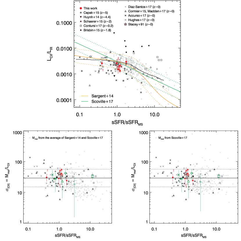
Figure 9: Correlation between the [C II]  luminosity and galaxies’ distance from the main-sequence. Top panel: [C II]-to-IR luminosity ratio as a function of the galaxy distance from the main sequence. The symbols are the same as reported in Figure 6 caption. Additionally, we include the average of the local star-forming galaxies from Stacey et al. (1991, cyan star). In particular, the sources by Brisbin et al. (2015) might be lensed, but the magnification factors are unknown and therefore we plot the observed values. We also show the running mean computed considering all the plotted datapoints a part from the sample from Contursi et al. (2017, black solid line). Finally we report the model by Sargent et al. (2014, yellow curve) and Scoville et al. (2017, green curve), showing the trend of the depletion time as a function of the sSFR, renormalized to match the observed $L_{\mathrm{[C~{}{\small II}]}}/L_{\mathrm{IR}}$ ratios (the standard deviations of the models are marked as dashed curves). Bottom panels: dependence of $\alpha_{\mathrm{[C~{}{\small II}]}}$ from galaxies’ distance from the main-sequence. The difference between the left and right panels concerns how the molecular gas mass was estimated for the sample of local galaxies from Diaz-Santos et al. (2017, light gray crosses). Since CO observations for this sample are not available, we estimated $M_{\mathrm{mol}}$, given the sSFR of each source, considering the relation between the depletion time and sSFR of galaxies. In the left panel we report the estimates obtained by averaging the trend reported by Sargent et al. (2014) and Scoville et al. (2017), whereas in the right panel we report the estimates obtained considering the trend by Scoville et al. (2017) only (see Section 3.3 for a more detailed discussion).

We considered samples with available sSFR measurements and in Figure 9 we plot the $L_{\mathrm{[C~{}{\small II}]}}/L_{\mathrm{IR}}$ ratio in bins of sSFR, normalized to the sSFR of the main-sequence at each redshift (Rodighiero et al., 2014). Our sample has a $L_{\mathrm{[C~{}{\small II}]}}/L_{\mathrm{IR}}$ ratio comparable to that reported in the literature for main-sequence galaxies at lower (Stacey et al. 1991, Cormier et al. 2015, the subsample of main-sequence galaxies from Diaz-Santos et al. 2017) and higher redshift (Capak et al. 2015). This is up to $\sim 10$ times higher than the typical $L_{\mathrm{[C~{}{\small II}]}}/L_{\mathrm{IR}}$ ratio of starbursts defined as to fall $>4$ times above the main-sequence (Rodighiero et al., 2011). Given the fact that the IR luminosity is commonly used as a SFR tracer and the [C II]  luminosity seems to correlate with the galaxies’ molecular gas mass, we expect the $L_{\mathrm{[C~{}{\small II}]}}/L_{\mathrm{IR}}$ ratio to depend on galaxies’ gas depletion time ($\tau_{\mathrm{dep}}=M_{\mathrm{mol}}/SFR$). This seems to be substantiated by the fact that the depletion time in main-sequence galaxies is on average $\sim$ 10 times higher than in starbursts (e.g. Sargent et al. 2014, Scoville et al. 2017), similarly to what is observed for the $L_{\mathrm{[C~{}{\small II}]}}/L_{\mathrm{IR}}$ ratio. To make this comparison more quantitative, we considered two models (Sargent et al. 2014, Scoville et al. 2017) predicting how the depletion time of galaxies changes as a function of their distance from the main-sequence and rescaled them to match the $L_{\mathrm{[C~{}{\small II}]}}/L_{\mathrm{IR}}$ observed for main-sequence galaxies. This scaling factor mainly depends on the [C II]-to-CO luminosity ratio and given the shift we applied to the Sargent et al. (2014) and Scoville et al. (2017) models we estimated $L_{\mathrm{[C~{}{\small II}]}}/L_{\mathrm{CO}}\sim 6000$. This is in good agreement with the typical values reported in the literature and ranging between 2000 – 10000 (Stacey et al. 1991, Magdis et al. 2014, Accurso et al. 2017a, Rigopoulou et al. 2018). We compare the rescaled models with observations in Figure 9. Given the higher number of main-sequence sources than starbursts, uncertainties on the estimate of stellar masses affecting galaxies sSFR would tend to systematically bias the distribution of $L_{\mathrm{[C~{}{\small II}]}}/L_{\mathrm{IR}}$ towards higher ratios as the distance from the main-sequence increases (similarly to the Eddington bias affecting source luminosities in surveys). To take this observational bias into account, we convolved the models by Sargent et al. (2014) and Scoville et al. (2017) with a Gaussian function with FWHM $\sim$ 0.2 dex (the typical uncertainty affecting stellar masses). Qualitatively, the drop of the depletion time that both models show with increasing sSFR well reproduces the trend of the [C II]-to-IR luminosity ratio with sSFR/sSFR_MS that is observed in Figure 9. Considering that $\tau_{\mathrm{dep}}=M_{\mathrm{mol}}$/SFR, and that the IR luminosity is a proxy for the SFR, the agreement between models and observations suggests that [C II]  correlates reasonably well with the molecular gas mass, keeping into account the limitations of this exercise (there are still lively ongoing debates on how to best estimate the gas mass of off main-sequence galaxies, as reflected in the differences in the models we adopted). In this framework, the [C II]  deficiency of starbursts can be explained as mainly due to their higher star formation efficiency, and hence far-UV fields, with respect to main-sequence sources. This is consistent with the invariance found by Graciá-Carpio et al. (2011), but it conceptually extends it to the possibility that [C II] is directly proportional to the molecular gas mass, at least empirically.

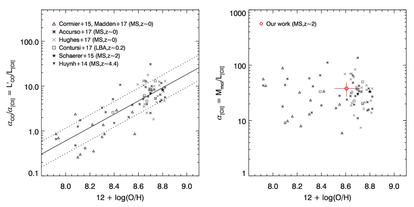
Figure 10: Metallicity dependence of $\alpha_{\mathrm{[C~{}{\small II}]}}$ for multiple samples with available metallicity estimate, all homogenized to the Pettini & Pagel (2004) calibration using the parametrizations by Kewley & Ellison (2008). The symbols are the same as reported in Figure 6 caption and legend. Left panel: ratio of the CO and [C II]  luminosity as a function of the galaxies gas phase metallicity. The linear fit of the two samples is reported (black solid line). Right panel: [C II]-to-H₂ conversion factor as a function of metallicity. The average measurement for our sample (red empty circle) is reported only in this panel since no CO measurements are available for our sources. The gas mass for our galaxies was estimated considering the integrated Schmidt-Kennicutt relation (see Section 2.4). We note that one of the galaxies by Cormier et al. (2015) is an outlier to the $L_{\rm[C~{}{\small II}]}$ – $M_{\rm mol}$ relation (and therefore of the $\alpha_{\rm[C~{}{\small II}]}$ – metallicity estimate) due to its very low [C II]  luminosity with respect to the CO one. We kept this galaxy in the sample for consistency with the literature, although there might be some issues with its [C II]  and/or CO measurements.

However, quantitatively some discrepancies between models and observations are present. The model by Sargent et al. (2014) accurately reproduces observations, at least up to sSFR/sSFR${}_{\mathrm{MS}}\sim 4$, but some inconsistencies are found at high sSFR/sSFR_MS. On the contrary, the model by Scoville et al. (2017) reproduces the observations for galaxies on and above the main-sequence, even if some discrepancies are present at sSFR/sSFR${}_{\mathrm{MS}}<1$, a regime that is not yet well tested (but see Schreiber et al. 2017b, Gobat et al. 2017a). Some possible explanations for the discrepancy between the observations and the model by Sargent et al. (2014) are the following: (i) starbursts might have higher gas fractions than currently predicted by the Sargent et al. (2014) model, in agreement with the Scoville et al. (2017) estimate; (ii) the [C II]  luminosity, at fixed stellar mass, is expected to increase with more intense radiation fields such as those characteristics of starbursts (Narayanan & Krumholz 2017, Diaz-Santos et al. 2017, Madden et al. in prep. 2017), possibly leading to too high [C II]-to-IR luminosity ratios with respect to the model by Sargent et al. (2014); (iii) if the fraction of [C II]  emitted by molecular gas decreases when the sSFR increases (e.g. for starbursts) as indicated by the model from Accurso et al. (2017b), then the [C II]-to-IR luminosity ratio would be higher than the expectations from the model by Sargent et al. (2014). However, to reconcile the observations of the most extreme starbursts (sSFR/sSFR${}_{\mathrm{MS}}\sim 10$) with the model, the [C II]  fraction emitted from molecular gas should drop to $\sim$ 30%, which is much lower than the predictions from Accurso et al. (2017b); (iv) we might also be facing an observational bias: starbursts with relatively high [C II]  luminosities might have been preferentially observed so far. Future deeper observations will allow us to understand if this mismatch is indeed due to an observational bias or if instead is real. In the latter case it would show that $\alpha_{\mathrm{[C~{}{\small II}]}}$ is not actually constant in the strong starburst regime.

We also notice that some local Lyman break analogs observed by Contursi et al. (2017) show $L_{\mathrm{[C~{}{\small II}]}}/L_{\mathrm{IR}}$ ratios higher than expected from both models, given their sSFR (Figure 9). Although these sources have sSFRs typical of local starbursts, their SFEs are main sequence-like as highlighted by Contursi et al. (2017). They are likely exceptional sources that do not follow the usual relation between sSFR and SFE. Given the fact that they show [C II]-to-IR luminosity ratios compatible with the average of main-sequence galaxies (Figure 6), we conclude that also in this case the SFE is the main parameter setting $L_{\mathrm{[C~{}{\small II}]}}/L_{\mathrm{IR}}$, suggesting that the [C II]  luminosity correlates with galaxies’ molecular gas mass.

3.4 Invariance of $\alpha_{\mathrm{[C~{}{\small II}]}}$ with gas phase metallicity

In this Section we investigate the dependence of the $\alpha_{\mathrm{[C~{}{\small II}]}}$ conversion factor on gas phase metallicity. Understanding whether [C II] traces the molecular gas also for low metallicity galaxies is relevant for observations of high-redshift galaxies that are expected to be metal-poor (Ouchi et al. 2013; Vallini et al. 2015).

In Figure 10 we show literature samples with available measurements of metallicity, CO, and [C II]  luminosities. To properly compare different samples we converted all metallicity estimates to the calibration by Pettini & Pagel (2004) using the parametrizations by Kewley & Ellison (2008). We converted the CO luminosity into gas mass by assuming the following $\alpha_{\mathrm{CO}}$ – metallicity dependence:

$$\log\alpha_{\mathrm{CO}}=0.64-1.5(12+\log(O/H)-8.7)$$ (4)

that yields the Galactic $\alpha_{\mathrm{CO}}$ for solar metallicities and has a slope in between those found in the literature (typically ranging between -1 and -2, e.g. Genzel et al. 2012, Schruba et al. 2012, Tan et al. 2014, Accurso et al. 2017a, Sargent et al. in prep. 2017). Adopting an $\alpha_{\mathrm{CO}}$ – metallicity dependence with a slope of $-1$ or $-2$ instead would not change our conclusions.

We show the ratio between the CO and [C II]  luminosity as a function of metallicity in Figure 10 (left panel). This plot was first shown by Accurso et al. (2017a) (see their Figure 2) and here we are adding some more literature datapoints. Over the metallicity range spanned by these samples ($12+\log\mathrm{O/H}\sim 7.8$ – 9), the CO luminosity drops by a factor 20 compared to [C II]. The fact that the $L^{\prime}_{\rm CO}/M_{\rm dust}$ ratio is overall constant with metallicity (given that both the gas-to-dust ratio and $\alpha_{\rm CO}$ similarly depend on metallicity) implies that $L_{[C~{}{\small II}]}/M_{\rm dust}$ has large variations with metallicity (similarly to the $L_{[C~{}{\small II}]}/L_{\rm CO}$ ratio), consistent with what discussed in Section 3.1 (namely that [C II] is not simply a dust mass tracer).

In Figure 10 (right panel) we show the $\alpha_{\mathrm{[C~{}{\small II}]}}$ dependence on metallicity. Although the scatter is quite large, the $L_{\mathrm{[C~{}{\small II}]}}/M_{\mathrm{mol}}$ ratio does not seem to depend on metallicity. When fitting the data with a linear function we obtain a slope of $-0.2\pm 0.2$, which is not significantly different from zero and consistent with a constant relation, and a standard deviation of 0.3 dex. This suggests that [C II]  can be used as a “universal” molecular gas tracer and a particularly convenient tool to empirically estimate the gas mass of starbursts (whose metallicity is notoriously difficult to constrain due to their high dust extinction) and high-redshift low-metallicity galaxies.

We note that the [C II]  luminosity is expected to become fainter at very low metallicities, due to the simple fact that less carbon is present (Cormier et al., 2015). However, this effect is negligible for the samples that we are considering and likely only becomes important at very low metallicities (12 + log(O/H) $<$ 8.0).

Table 4: Estimates of the [C II]-to H₂ conversion factor.

Samples	Mean	Standard deviation	Median	M.A.D.
	[M⊙/L⊙]	[dex]	[M⊙/L⊙]	[dex]
(1)	(2)	(3)	(4)	(5)
All	31	0.3	31	0.2
Local	30	0.3	28	0.2
High-$z$	35	0.2	38	0.1

Columns (1) Samples used to compute $\alpha_{\mathrm{[C~{}{\small II}]}}$. For the local estimate we considered the Accurso et al. (2017a) and Cormier et al. (2015) datasets, whereas for the high-redshift one we used our measurements together with those by Capak et al. (2015). The global estimate of $\alpha_{\mathrm{[C~{}{\small II}]}}$ was done by considering all the aforementioned samples.; (2) mean $\alpha_{\mathrm{[C~{}{\small II}]}}$; (3) standard deviation of the $\alpha_{\mathrm{[C~{}{\small II}]}}$ estimates; (4) median $\alpha_{\mathrm{[C~{}{\small II}]}}$; (5) mean absolute deviation of $\alpha_{\mathrm{[C~{}{\small II}]}}$ estimates.

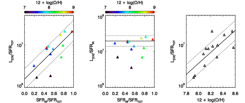
Figure 11: [C II]  dependence on the galaxies’ total (UV + IR) and obscured (IR only) SFR. The sample is made of the low-metallicity sources by Cormier et al. (2015), Madden et al. in prep. (2017). Left panel: dependence of the [C II]  luminosity to total SFR ratio on the ratio between the total and obscured SFR. The fit of the data is reported (solid black line) together with the standard deviation of the data (dashed black line). Central panel: dependence of the [C II]  luminosity to obscured SFR ratio on the ratio between the total and obscured SFR. The average ratio for our $z\sim 2$ sample of main-sequence galaxies is reported (solid black line) together with its uncertainty (dashed black line). Right panel: dependence of the [C II]  luminosity to total SFR on the gas phase metallicity. The fit of the data is reported (solid black line) together with the standard deviation of the data (dashed black line).

3.5 Implications for surveys at $z>2$

As shown in the previous Sections, [C II]  correlates with the galaxies’ molecular gas mass, and the [C II]-to-H₂ conversion factor is likely independent of the main-sequence and starburst behaviour of galaxies, as well as of their gas phase metallicity. In perspective, this is particularly useful for studies of high-redshift targets. At high redshift in fact, due to the galaxies’ low metallicity, CO is expected not to trace the bulk of the H₂ anymore (e.g. Maloney & Black 1988, Madden et al. 1997, Wolfire et al. 2010, Bolatto et al. 2013). Thanks to its high luminosity even in the low metallicity regime, [C II]  might become a very useful tool to study the ISM properties at these redshifts. However some caution is needed when interpreting or predicting the [C II]  luminosity at high redshift. Recent studies have shown that low-metallicity galaxies have low dust content, hence the UV obscuration is minimal and the IR emission is much lower than in high-metallicity sources (e.g. Galliano et al. 2005, Madden et al. 2006, Rémy-Ruyer et al. 2013, De Looze et al. 2014, Cormier et al. 2015). This means that the obscured star formation rate – that can be computed from the IR luminosity through the calibration done by Kennicutt (1998) – can be up to 10 times lower than the unobscured one (e.g. computed thorough the UV SED fitting). This can be seen also in Figure 11 where we report the sample of local low-metallicity galaxies from Cormier et al. (2015) and Madden et al. in prep. (2017), taking at face value the SFR estimates from the literature. The $SFR_{\rm IR}/SFR_{\rm TOT}$ ratio clearly depends on the galaxies’ metallicity, with the most metal-poor showing on average lower ratios. Furthermore, the ratio between the [C II]  luminosity and the total SFR of these galaxies linearly depends on the $SFR_{\rm IR}/SFR_{\rm TOT}$ ratio (Figure 11, left panel):

$$\log(L_{\rm[C~{}{\small II}]}/SFR_{\rm TOT})=6.2(\pm 0.2)+1.1(\pm 0.3)SFR_{\rm IR}/SFR_{\rm TOT}$$ (5)

with a scatter of 0.2 dex, indicating that galaxies with lower metallicity (and lower obscured SFR) typically have lower $L_{\rm[C~{}{\small II}]}/SFR_{\rm TOT}$ ratios. This is clearly visible in Figure 11 (right panel): the dependence of the $L_{\rm[C~{}{\small II}]}/SFR_{\rm TOT}$ ratio on metallicity can be parametrized as follows:

$$\log(L_{\rm[C~{}{\small II}]}/SFR_{\rm TOT})=-3.8(\pm 2.8)+1.3(\pm 0.3)[12+\log(O/H)]$$ (6)

with a dispersion of 0.2 dex. On the contrary, the ratio between the [C II]  luminosity and the obscured SFR is constant with the $SFR_{\rm IR}/SFR_{\rm TOT}$ ratio (Figure 11, central panel). This suggests that the [C II]  emission is related to dusty star-forming regions rather than to the whole SFR of the galaxy. At very high redshift (e.g. $z>4$) measuring the IR luminosity is problematic and therefore often the total SFR obtained from UV-corrected estimates is used to derive a measurement of $L_{\rm IR}$. However, this might lead to overestimate the IR luminosity and therefore bias the [C II]-to-IR luminosity ratio toward lower values. This would mean that the [C II]  deficit observed at high redshift might be due to the approximate estimate of the IR luminosity and not only due to the real evolution of the ISM properties. It could also explain the several cases of $z>5$ galaxies with [C II]  non-detections that have been recently reported (Combes et al. 2012, Ouchi et al. 2013, Maiolino et al. 2015, Schaerer et al. 2015, Watson et al. 2015): if the total SFR was used to estimate the $L_{\rm IR}$ and the typical $L_{\rm[C~{}{\small II}]}/L_{IR}=2\times 10^{-3}$ ratio was used to predict the [C II]  luminosity when proposing for observing time, the $L_{\rm[C~{}{\small II}]}$ would have been overestimated and therefore the observations would have not been deep enough to detect the [C II]  emission of the targets. Future actual measurements of the IR luminosity will be crucial to assess whether high-redshift observations were biased, or on the contrary if the [C II]  deficiency is due to an actual evolution of galaxies’ properties from $z\sim 0$ to $z\sim 5$. In the latter case the reason for the deficiency might still not be clear and an additional word of caution is needed: if the [C II]  luminosity traces the molecular gas mass even at these high redshifts, these sources might be [C II]  deficient due to a low molecular gas content and high SFE. However, the different conditions of the ISM at these redshifts, the lower dust masses, and likely the much harder radiation fields might play an important role as well, potentially introducing systematics and limiting the use of [C II]  as molecular gas tracer for very distant galaxies.

3.6 Caveats

Finally we mention a few caveats that it is important to consider when using the [C II]  emission line to trace galaxies’ molecular gas.

First, as discussed in Section 3.5, at redshift $z\gtrsim 5$ the ISM conditions are likely different with respect to lower redshift (e.g. lower dust masses, harder radiation fields). This might impact the [C II]  luminosity, possibly introducing some biases, and limiting the use of the [C II]  emission line to estimate the molecular gas mass of galaxies at very high redshift.

Secondly, there are local studies indicating that [C II], mainly due to its low ionization potential, is simultaneously tracing the molecular, atomic and ionized phases (e.g. Stacey et al. 1991, Sargsyan et al. 2012, Rigopoulou et al. 2014, Diaz-Santos et al. 2017, Croxall et al. 2017). The total measured [C II]  luminosity might therefore be higher than the one arising from the molecular gas only: this would lead to overestimated H₂ masses. However, it seems that 70% – 95% of the [C II]  luminosity originates from PDRs (Cormier et al. 2015, Diaz-Santos et al. 2017) and in particular $>75$% arises from the molecular phase (Pineda et al. 2013, Velusamy & Langer 2014, Vallini et al. 2015, Olsen et al. 2017, Accurso et al. 2017b).

Lastly, as opposed to CO, [C II]  is likely emitted only in regions where star formation is ongoing. Molecular clouds that are not illuminated by young stars would therefore not be detected (Beuther et al., 2014).

All in all, the limitations affecting [C II]  seem to be different with respect to the ones having an impact on the molecular gas tracers commonly used so far (CO, [C I], or dust measurements), making it an independent molecular gas proxy. Future works comparing the gas mass estimates obtained with different methods will help understanding what tracer is better to consider depending on the physical conditions of the target.

4 Conclusions

In this paper we discuss the analysis of a sample of 10 main-sequence galaxies at redshift $z\sim 2$ in GOODS-S. We present new ALMA Band 7 850 $\mu$m observer frame continuum, and Band 9 [C II]  line together with 450 $\mu$m observer frame continuum observations, complemented by a suite of ancillary data, including HST, Spitzer, Herschel, and VLA imaging, plus VLT and Keck longslit spectroscopy. The goal is to investigate whether $z\sim 2$, main-sequence galaxies are [C II]  deficient and understand what are the main physical parameters affecting the [C II]  luminosity. We summarize in the following the main conclusions we reached.

• The ratio between the [C II]  and IR luminosity ($L_{\mathrm{[CII]}}/L_{\mathrm{IR}}$) of $z\sim 2$ main-sequence galaxies is $\sim 2\times 10^{-3}$, comparable to that of local main-sequence sources and a factor of $\sim 10$ higher than local starbursts. This implies that there is not a unique correlation between $L_{\mathrm{[C~{}{\small II}]}}$ and L_IR and therefore we should be careful when using the [C II]  luminosity as a SFR indicator. Similarly, the [C II]  luminosity does not uniquely correlate with galaxies’ specific star formation rate, intensity of the radiation field, and dust mass.

• The [C II] emission is spatially extended, on average, on scales comparable to the stellar mass sizes (4 – 7 kpc), as inferred from HST imaging in the optical rest frame. This is in agreement with the results by Stacey et al. (2010), Hailey-Dunsheath et al. (2010), and Brisbin et al. (2015) who, for samples of $z\sim 1$ – 2 galaxies, find similar [C II]  extensions. This also suggests that our sample of main sequence galaxies, with typical stellar masses and SFRs, is not made up of the ultra-compact (and more massive) sources selected and studied by Tadaki et al. (2015) and Barro et al. (2016).

• The [C II]  luminosity linearly correlates with galaxies’ molecular gas masses. By complementing our sample with those from the literature, we constrained the $L_{\mathrm{[C~{}{\small II}]}}$-to-H₂ conversion factor: it has a median $\alpha_{\mathrm{[C~{}{\small II}]}}=31$ M_⊙/L_⊙ and a median absolute deviation of $\sim$ 0.2 dex. We find it mostly invariant with galaxies’ redshift, depletion time, and gas phase metallicity. This makes [C II]  a convenient emission line to estimate the gas mass of starbursts, a notoriously hard property to constrain by using the CO and dust emission due to the large uncertainties in the conversion factors to be adopted. Furthermore, the invariance of $\alpha_{\mathrm{[C~{}{\small II}]}}$ with metallicity together with the remarkable brightness of [C II]  makes this emission line a useful tool to constrain gas masses at very high redshift, where galaxies’ metallicity is expected to be low.

• Considering that [C II]  traces the molecular gas and the IR luminosity is a proxy for SFR, the $L_{\rm[C~{}{\small II}]}/L_{\rm IR}$ ratio seems to be mainly a tracer of galaxies’ gas depletion time. The $L_{\rm[C~{}{\small II}]}/L_{\rm IR}$ ratio for our sample of $z\sim 2$ main-sequence galaxies is $\sim$ 1.5 times lower than that of local main-sequence samples, as expected from the evolution of depletion time with redshift.

• The weak [C II] signal from $z>6$ – 7 galaxies and the many non-detections in the recent literature might be evidence of high star formation efficiency, but might be also due to the fact that the expected signal is computed from the total UV star formation rate, while local dwarfs suggest that [C II] only reflects the portion of SFR reprocessed by dust in the IR.

• Although some caveats are present (e.g. [C II]  non-detections at very high redshift might also be due to the effects of a strong radiation field; [C II]  might be tracing different gas phases simultaneously; it is only emitted when the gas is illuminated by young stars, so it only traces molecular gas with ongoing star formation), the limitations that affect [C II]  are different with respect to those impacting more traditional gas tracers such as CO, [C I], and dust emission. This makes [C II]  an independent proxy, particularly suitable to push our current knowledge of galaxies’ ISM to the highest redshifts.

Appendix A A. Resolution

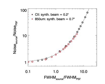
Figure 12: Analysis of how the flux uncertainty (noise) changes when a source is resolved, with respect to the unresolved case. The noise obtained fitting an emission line with a Gaussian model normalized by that retrieved with a PSF fit is reported as a function of the source’s size normalized by that of the beam. The fit of the datapoints is reported gray solid line. Normalized in this way, the trend is independent on the resolution of the observations and expected to hold quite generally for ALMA observations, at least at first order (to a second order, it should depend on the exact baseline distributions in the observing configuration).

From the HST optical images we estimated that our sample galaxies have FWHM sizes of $\sim$ 0.7 – 1” (see Section 2.1). Since we wanted to measure total [C II]  fluxes, we asked for ALMA observations choosing the configuration C32-1, to get a resolution of $\sim$ 1”. However, the data were taken with the configuration C32-3 instead, providing a $\sim$ 0.2” resolution, higher than needed, and a maximum recoverable scale of $\sim$ 3.5”: our galaxies are then spatially resolved. We tested the impact of the resolution on our flux and size estimates as follows. With the CASA task simobserve we simulated 2D Gaussians with increasing FWHM (in the range 0.1” – 2”), mimicking observations taken with $\sim$ 0.2” resolution. We then fitted these mock data in the uv plane with the task uvmodelfit. Both sizes and fluxes are very well recovered even for large galaxies provided the data had large enough S/N. Very similar results are obtained when simulating sources with GILDAS instead of CASA.

Although fluxes and sizes are well estimated when fitting the emission lines in the uv plane almost independently of the adopted ALMA configuration, the S/N of the observations dramatically decreases when the sources are resolved. To quantify it, we considered the galaxy in our sample showing the highest S/N [C II]  emission line (ID9347). We fitted its velocity-integrated map multiple times with the GILDAS algorithm, first with a point source model and then adopting a Gaussian profile with increasing FWHM. In the following we call “noise” the uncertainty associated with the flux, as estimated by GILDAS during the fitting procedure. In Figure 12 we illustrate how the noise of an extended source changes when it is resolved out. The noise is estimated as the uncertainty associated with the flux, when fitting the data. We repeated the exercise for both the [C II]  emission line (synthesised beam $\sim$ 0.2”) and the 850 $\mu$m continuum (synthesised beam $\sim$ 0.7”). By fitting the datapoints with a polynomial curve we obtained the following relation:

$$y=1.00+0.79x+0.14x^{2}+0.01x^{3}$$ (7)

where $y$ is the ratio of the source and PSF uncertainties ($y=\mathrm{Noise_{source}}/\mathrm{Noise_{PSF}}$), and $x$ is the ratio of their FWHM ($x=\mathrm{FWHM_{source}}/\mathrm{FWHM_{PSF}}$).

Figure 12 might be of particular interest when proposing for observations, since the ALMA calculator only provides sensitivity estimates assuming that the source is unresolved. Our plots allow to rescale the sensitivity computed by the calculator on the basis of the actual FWHM of the target, and therefore to estimate the correct S/N to be expected in the observations. We notice however that these predictions assume that the correct position and FWHM of the source are known.

Appendix B B. Astrometry

When comparing our optical data with the observations of the [C II]  emission lines together with the 450 $\mu$m (Band 9) and 850 $\mu$m (Band 7) continuum, there is an astrometric offset between HST and ALMA images. Considering only the galaxies with a line and/or continuum detection (S/N $>$ 3), we estimated the average offsets needed to align the luminosity peak of the HST and ALMA datasets. We measured a systematic shift of the HST centroid with respect to the ALMA data of $\sim-$ 0.2” in declination and a non significant, negligible offset of $\sim$ 0.06” in right ascension.

We acknowledge that the astrometry offsets between HST and ALMA datasets in GOODS-S are a known issue (Dunlop et al. 2017, Rujopakarn et al. 2016, Barro et al. 2016, Aravena et al. 2016b, Cibinel et al. 2017). Our estimate is consistent with the ones reported in the literature. A detailed map of the astrometry offset of the HST imaging in GOODS-S will be provided by Dickinson et al. in prep. (2017).

In our analysis we adopt the following coordinate shifts $\Delta RA=0$”, $\Delta DEC=-0.2$”.

Appendix C C. Literature data

We briefly describe the literature samples that we used to complement our observations and the methods used to derive the parameters considered in our analysis (redshift, [C II]  luminosity, IR luminosity, CO luminosity, molecular gas mass, specific star formation rate, and metallicity). To properly compare different samples we converted all metallicity estimates to the calibration by Pettini & Pagel (2004) using the parametrizations by Kewley & Ellison (2008). Also we homogenized all the IR luminosities reporting them to the 8 – 1000 $\mu$m range.

• Local dwarf galaxies (Cormier et al. 2015, Madden et al. in prep. 2017). Sample of local dwarf galaxies observed with Herschel/PACS and SPIRE as part of the DGS survey (Madden et al., 2013). They have metallicity ranging from $\sim$ 1/40 Z_⊙ to near solar, SFR from $\sim 5\times 10^{-4}$ M_⊙ yr^-1 to 25 M_⊙ yr^-1 and they are all nearby (maximum distance $\sim$ 200 Mpc). In this work we only consider the galaxies that have been followed-up with ATNF Mopra 22–m, APEX, and IRAM 30–m telescopes and show a CO(1-0) emission line detection (Cormier et al. 2014, Madden et al. in prep. 2017, De Vis et al. 2017). We converted the CO luminosity of these sources (Cormier et al. 2014, Madden et al. in prep. 2017) into molecular gas mass by using a conversion factor that depends on metallicity ($\alpha_{\mathrm{CO}}\sim Z^{-1.5}$, see Section 3.4). Their IR luminosity was estimated fitting the IR SEDs with semi-empirical models (Galliano et al., 2011). Rémy-Ruyer et al. (2014) estimated their SFR from the total infrared luminosity using the equation from Kennicutt (1998) and their stellar mass from the 3.6 and 4.5 $\mu$m flux densities using the formula of Eskew et al. (2012).

• Local main-sequence galaxies (Accurso et al., 2017a). Sample of intermediate mass ($9<\log M_{\star}/M_{\odot}<10$), local galaxies from the xCOLD GASS survey (Saintonge et al., 2017) with metallicities in the range $0.4<Z/Z_{\odot}<1.0$. They have Herschel [C II]  and IRAM CO(1-0) observations, together with auxiliary data from GALEX, WISE, and SDSS. Accurso et al. (2017a) computed the molecular gas masses from the CO luminosity, considering a conversion factor that depends on metallicity ($\alpha_{\mathrm{CO}}\sim Z^{-1.5}$, see Section 3.4). Saintonge et al. (2016) measured the SFR of these sources from the combination of UV and IR photometry and their stellar mass from SDSS photometry.

• Local main-sequence galaxies (Stacey et al., 1991). Sample of local galaxies with KAO observations. We excluded those that were classified as starbursts (on the basis of their dust temperature: $T_{\mathrm{dust}}\geq 40$ K) and considered only the 6 “normal” star-forming ones. CO observations taken with a similar beam size to the [C II]  ones are reported by Stacey et al. (1991). We estimate the molecular gas mass for these galaxies considering a Milky-Way like $\alpha_{\mathrm{CO}}=4.4$ K km s^-1 pc² conversion factor. Measurements of stellar masses, and metallicity are not available. In Figure 9 we report the average [C II]-to-IR luminosity ratio of these 6 sources considering that they are in main-sequence ($sSFR/sSFR_{\mathrm{MS}}=1$).

• Local main-sequence and starburst galaxies (Brauher et al., 2008). Sample of local galaxies observed with ISO/LWS including “normal” star-forming systems, starbursts, and AGNs. In this analysis we only considered the 74 sources with both [C II]  and IR detection. The IR luminosity was estimated from the 25 $\mu$m, 60 $\mu$m, and 100 $\mu$m fluxes as reported by Brauher et al. (2008). Molecular gas and stellar mass, and metallicity measurements are not available.

• Local starbursts (Díaz-Santos et al. 2013, Diaz-Santos et al. 2017). Sample of local luminous infrared galaxies observed with Herschel/PACS as part of GOALS (Armus et al., 2009). They have far-infrared luminosities in the range $2\times 10^{9}$ L_⊙ – $2\times 10^{12}$ L_⊙ and sSFR $5\times 10^{-12}$ – $3\times 10^{-9}$ yr^-1. No measurements of their molecular gas mass are available from the literature. We therefore estimated $M_{\rm mol}$ considering the models by Sargent et al. (2014) and Scoville et al. (2017) that parametrize the dependence of galaxies’ depletion time on their sSFR (see Section 3.3 for more details). The IR luminosity was estimated from the 60 $\mu$m and 100 $\mu$m as reported by Díaz-Santos et al. (2013). Their SFR is estimated from IR luminosity (Kennicutt, 1998) and their stellar mass from the IRAC 3.6 $\mu$m and Two Micron All Sky Survey (2MASS) K-band photometry (Howell et al., 2010). The metallicity of these sources is not available.

• Redshift $z\sim 0.2$ Lyman break analogs (Contursi et al., 2017). Sample of Lyman break analogs (namely, compact galaxies with UV luminosity $L_{\mathrm{UV}}>2\times 10^{10}$ L_⊙ and UV surface brightness $I_{\mathrm{1530\AA}}>10^{9}$ L_⊙ kpc^-2) at redshift 0.1 – 0.3, with Herschel/PACS [C II]  and IRAM CO(1-0) observations. Their IR luminosity was derived by fitting the IR SEDs of these sources with Draine & Li (2007) models. Their SFRs span the range 3 – 100 M_⊙ yr^-1 and their sSFR are comparable to those of $z\sim 2$ main-sequence galaxies. We determined their molecular gas mass from the CO luminosity, using a conversion factor that depends on metallicity ($\alpha_{\mathrm{CO}}\sim Z^{-1.5}$, see Section 3.4). Their SFR has been derived from the IR luminosity considering the equation from Kennicutt (1998) and their stellar masses from rest-frame optical photometry (Overzier et al., 2009).

• Redshift $z\sim 0.5$ starbursts (Magdis et al., 2014). Sample of (ultra)-luminous infrared galaxies at redshift 0.21 – 0.88 observed with Herschel. They have an IR luminosity $L_{\mathrm{IR}}>10^{11.5}$ L_⊙. Among them, 5 are classified as AGN host, QSO, or composite systems from optical or IRS data. The gas mass has been estimated from the CO luminosity considering a conversion factor that depends on metallicity ($\alpha_{\mathrm{CO}}\sim Z^{-1.5}$, see Section 3.4). Their IR luminosity was estimated fitting the IR SEDs of these sources with Draine & Li (2007) models. The SFR of these sources is derived from the IR luminosity considering the equation from Kennicutt (1998).

• Redshift z = 1.8 lensed galaxy (Ferkinhoff et al., 2014). Single galaxy lensed by the foreground galaxy observed with Herschel and CSO/ZEUS. The gas mass of this galaxy was determined from the CO luminosity considering a conversion factor $\alpha_{\mathrm{CO}}=4.4$ M_⊙ (K km s${}^{-}1$ pc²)^-1. Its IR luminosity was estimated fitting the IR SED with Siebenmorgen & Krügel (2007) models. In the following we report the unlensed luminosities.

• Redshift z = 1.8 main-sequence galaxies (Brisbin et al., 2015). Sample of galaxies at redshift $z\sim 1.8$ observed with CSO/ZEUS. The observed IR luminosity of these sources ranges between $7\times 10^{11}$ L_⊙ – $6\times 10^{12}$ L_⊙ and was estimated fitting the IR SED with the models by Dale & Helou (2002). Measurements of molecular gas masses are not available. The star formation rate has been estimated from the IR luminsity, considering the equation from Kennicutt (1998). The stellar mass has been estimated from the 2 $\mu$m IRAC flux (Magdis et al., 2010). Metallicity measurements are not available. We note that some of the galaxies by Brisbin et al. (2015) might be lensed. While the L${}_{\mathrm{[C~{}{\small II}]}}$/L_IR ratio should not be particularly affected by differential magnification, the absolute [C II]  and IR luminosities might instead be amplified.

• Redshift z = 2 lensed main-sequence galaxy (Schaerer et al., 2015). Single galaxy lensed by the foreground galaxy cluster MACS J0451+0006 observed with HST, Spitzer, Herschel, PdBI, and ALMA. The gas mass of this galaxy was determined from the CO luminosity considering a conversion factor that depends on metallicity ($\alpha_{\mathrm{CO}}\sim Z^{-1.5}$, see Section 3.4). Dessauges-Zavadsky et al. (2015) estimated its IR luminosity fitting the IR SED with Draine & Li (2007) models and derived its SFR and stellar mass from the best energy conserving SED fits, obtained under the hypothesis of an extinction fixed at the observed IR-to-UV luminosity ratio following the prescriptions of Schaerer et al. (2013).

• Redshift $z\sim 1$ – 2 main-sequence and starbursts (Stacey et al., 2010). Sample of galaxies at redshift 1 – 2 observed with CSO/ZEUS. The observed far-IR luminosity of these sources ranges between $3\times 10^{12}$ L_⊙ – $2.5\times 10^{14}$ L_⊙, although two of them are lensed. In the following we report the observed luminosities since the magnification factors are generally very uncertain or unknown. Both AGN and star-forming galaxies are included. Measurements of molecular gas masses are not available, as well as estimates of the sources’ stellar mass, and metallicity. The IR luminosity was estimated from the 12 $\mu$m, 25 $\mu$m, 60 $\mu$m, and 100 $\mu$m fluxes as reported by Stacey et al. (2010).

• Redshift $z=4.44$ main-sequence galaxy (Huynh et al., 2014). Single galaxy observed with ATCA, ALMA, Herschel, and HST. The gas mass of this galaxy was determined from the CO luminosity considering a conversion factor that depends on metallicity ($\alpha_{\mathrm{CO}}\sim Z^{-1.5}$, see Section 3.4). Huynh et al. (2014) estimated its IR luminosity fitting the IR SED with Chary & Elbaz (2001) models. Its SFR was derived from the IR luminosity following the calibration from Kennicutt (1998) and its stellar mass from the H-band magnitude together with an average mass-to-light ratio for a likely sub-millimeter galaxy star formation history (Swinbank et al., 2012).

• Redshift $z\sim 5.5$ main-sequence galaxies (Capak et al., 2015). Sample of star-forming galaxies at redshift 5 – 6 observed with ALMA and Spitzer. In the following we only report the 4 galaxies with detected [C II]  emission together with the average [C II]  luminosity obtained by stacking the 6 non-detections. Two galaxies were also serendipitously detected in [C II]  and added to the sample. The SFRs range between 3 – 169 M_⊙ yr^-1 and the stellar masses $9.7<\log M_{\star}/M_{\odot}<10.8$. CO observations are not available, so we estimated the molecular gas masses using the integrated Schmidt-Kennicutt relation for main-sequence galaxies reported by Sargent et al. (2014). The IR luminosity was estimated using the grey body models from Casey (2012). Capak et al. (2015) estimated the SFR of the sources by summing the UV and IR luminosity and the stellar mass by fitting SED models to the UV to IR photometry. The metallicity of these galaxies is not available.

• Redshift $z\sim 2$ – 6 lensed galaxies (Gullberg et al., 2015). Sample of strongly lensed dusty star-forming galaxies in the redshift range 2.1 – 5.7 selected from the South Pole Telescope survey (Vieira et al. 2010, Carlstrom et al. 2011) on the basis of their 1.4 mm flux ($S_{\mathrm{1.4mm}}>20$ mJy) and followed-up with ALMA and Herschel/SPIRE. Among them, 11 sources also have low-$J$ CO detections from ATCA. In the following we report the de-magnified luminosities, where the magnification factors are taken from (Spilker et al., 2016). The molecular gas mass has been computed considering the CO luminosity and an $\alpha_{\mathrm{CO}}$ conversion factor derived for each source on the basis of their dynamical mass (see Aravena et al. 2016a for more details). The adopted $\alpha_{\mathrm{CO}}$ factors have values in the range 0.7 – 12.3 M_⊙ K km s^-1 pc^-2. Their IR luminosity was estimated fitting the IR SEDs of these sources with greybody models from Greve et al. (2012). The stellar mass, and metallicity of these galaxies are not available.

Table 5: Compilation of literature data used in this paper. The full table is available online.

ID	z	L${}_{\mathrm{[C~{}{\small II}]}}$	LIR	L’CO	Mmol	sSFR	12 + log(O/H)
		[L⊙]	[L⊙]	[L⊙]	[M⊙]	[yr-1]
Local dwarf galaxies (Cormier et al. 2015, Madden et al. in prep. 2017)
Haro11	0.021	$1.3\times 10^{8}$	$1.9\times 10^{11}$	$9.8\times 10^{7}$	$1.7\times 10^{9}$	$1.4\times 10^{-9}$	8.30
Haro2	0.005	$1.4\times 10^{7}$	$6.0\times 10^{9}$	$4.1\times 10^{7}$	$4.8\times 10^{8}$	$2.2\times 10^{-10}$	8.42
Haro3	0.005	$1.3\times 10^{7}$	$5.2\times 10^{9}$	$1.9\times 10^{7}$	$4.3\times 10^{8}$	$2.0\times 10^{-10}$	8.22
He2-10	0.002	$1.1\times 10^{7}$	$5.2\times 10^{9}$	$3.0\times 10^{7}$	$2.2\times 10^{8}$	$1.7\times 10^{-10}$	8.55
IIZw40	0.003	$1.9\times 10^{6}$	$2.7\times 10^{9}$	$1.6\times 10^{6}$	$1.1\times 10^{8}$	$2.8\times 10^{-9}$	7.92

Columns (1) Galaxy ID; (2) Redshift; (3) [C II]  luminosity; (4) Infrared luminosity; (5) CO luminosity; (6) Molecular gas mass; (7) Specific star formation rate; (8) Gas-phase metallicity.
Notes. For the sample by Díaz-Santos et al. (2013), Diaz-Santos et al. (2017) we report two molecular gas mass estimates. They have both been obtained considering the sSFR of each galaxy, their SFR, and the relation between depletion time and sSFR (Sargent et al. 2014, Scoville et al. 2017). The difference between the two estimates consists in the model that we assumed: the first is derived using the mean depletion time obtained averaging the parametrization by Sargent et al. (2014) and Scoville et al. (2017), whereas the second is estimated considering only the model by Scoville et al. (2017, see Section 3.3 for a more detailed discussion).

References

- Abel et al. (2009) Abel N. P., Dudley C., Fischer J., Satyapal S., van Hoof P. A. M., 2009, ApJ, 701, 1147
- Accurso et al. (2017a) Accurso G., et al., 2017a, preprint, (arXiv:1702.03888)
- Accurso et al. (2017b) Accurso G., Saintonge A., Bisbas T. G., Viti S., 2017b, MNRAS, 464, 3315
- Amorín et al. (2016) Amorín R., Muñoz-Tuñón C., Aguerri J. A. L., Planesas P., 2016, A&A, 588, A23
- Aravena et al. (2016a) Aravena M., et al., 2016a, MNRAS, 457, 4406
- Aravena et al. (2016b) Aravena M., et al., 2016b, ApJ, 833, 68
- Armus et al. (1987) Armus L., Heckman T., Miley G., 1987, AJ, 94, 831
- Armus et al. (2009) Armus L., et al., 2009, PASP, 121, 559
- Barro et al. (2016) Barro G., et al., 2016, ApJ, 827, L32
- Béthermin et al. (2010) Béthermin M., Dole H., Cousin M., Bavouzet N., 2010, A&A, 516, A43
- Béthermin et al. (2015) Béthermin M., et al., 2015, A&A, 573, A113
- Beuther et al. (2014) Beuther H., et al., 2014, A&A, 571, A53
- Bigiel et al. (2008) Bigiel F., Leroy A., Walter F., Brinks E., de Blok W. J. G., Madore B., Thornley M. D., 2008, AJ, 136, 2846
- Bolatto et al. (2013) Bolatto A. D., Wolfire M., Leroy A. K., 2013, ARA&A, 51, 207
- Bothwell et al. (2016) Bothwell M. S., Maiolino R., Peng Y., Cicone C., Griffith H., Wagg J., 2016, MNRAS, 455, 1156
- Bournaud et al. in prep. (2017) Bournaud, F. et al. in prep. 2017
- Bouwens et al. (2012) Bouwens R. J., et al., 2012, ApJ, 754, 83
- Brauher et al. (2008) Brauher J. R., Dale D. A., Helou G., 2008, ApJS, 178, 280
- Brisbin et al. (2015) Brisbin D., Ferkinhoff C., Nikola T., Parshley S., Stacey G. J., Spoon H., Hailey-Dunsheath S., Verma A., 2015, ApJ, 799, 13
- Brisbin et al. (2017) Brisbin D., et al., 2017, A&A, 608, A15
- Bruzual & Charlot (2003) Bruzual G., Charlot S., 2003, MNRAS, 344, 1000
- Bushouse et al. (2002) Bushouse H. A., et al., 2002, ApJS, 138, 1
- Calzetti et al. (2000) Calzetti D., Armus L., Bohlin R. C., Kinney A. L., Koornneef J., Storchi-Bergmann T., 2000, ApJ, 533, 682
- Capak et al. (2015) Capak P. L., et al., 2015, Nature, 522, 455
- Carilli & Walter (2013) Carilli C. L., Walter F., 2013, ARA&A, 51, 105
- Carlstrom et al. (2011) Carlstrom J. E., et al., 2011, PASP, 123, 568
- Casey (2012) Casey C. M., 2012, MNRAS, 425, 3094
- Chabrier (2003) Chabrier G., 2003, PASP, 115, 763
- Chary & Elbaz (2001) Chary R., Elbaz D., 2001, ApJ, 556, 562
- Cibinel et al. (2015) Cibinel A., et al., 2015, ApJ, 805, 181
- Cibinel et al. (2017) Cibinel A., et al., 2017, MNRAS, 469, 4683
- Cimatti et al. (2002) Cimatti A., et al., 2002, A&A, 392, 395
- Combes et al. (2012) Combes F., et al., 2012, A&A, 538, L4
- Combes et al. (2013) Combes F., García-Burillo S., Braine J., Schinnerer E., Walter F., Colina L., 2013, A&A, 550, A41
- Contursi et al. (2017) Contursi A., et al., 2017, preprint, (arXiv:1706.04107)
- Coogan et al. (2018) Coogan R., et al., 2018, 479,703C
- Cormier et al. (2014) Cormier D., et al., 2014, A&A, 564, A121
- Cormier et al. (2015) Cormier D., et al., 2015, A&A, 578, A53
- Croxall et al. (2017) Croxall K. V., et al., 2017, ApJ, 845, 96
- Daddi et al. (2007) Daddi E., et al., 2007, ApJ, 670, 156
- Daddi et al. (2010) Daddi E., et al., 2010, ApJ, 713, 686
- Daddi et al. (2015) Daddi E., et al., 2015, A&A, 577, A46
- Dale & Helou (2002) Dale D. A., Helou G., 2002, ApJ, 576, 159
- Davé et al. (2012) Davé R., Finlator K., Oppenheimer B. D., 2012, MNRAS, 421, 98
- De Looze et al. (2010) De Looze I., et al., 2010, A&A, 518, L54
- De Looze et al. (2014) De Looze I., et al., 2014, A&A, 568, A62
- De Vis et al. (2017) De Vis P., et al., 2017, MNRAS, 471, 1743
- Dessauges-Zavadsky et al. (2015) Dessauges-Zavadsky M., et al., 2015, A&A, 577, A50
- Díaz-Santos et al. (2013) Díaz-Santos T., et al., 2013, ApJ, 774, 68
- Diaz-Santos et al. (2017) Diaz-Santos T., et al., 2017, preprint, (arXiv:1705.04326)
- Dickinson et al. in prep. (2017) Dickinson, M. et al. in prep. 2017
- Draine & Li (2007) Draine B. T., Li A., 2007, ApJ, 657, 810
- Dunlop et al. (2017) Dunlop J. S., et al., 2017, MNRAS, 466, 861
- Elbaz et al. (2007) Elbaz D., et al., 2007, A&A, 468, 33
- Elbaz et al. (2011) Elbaz D., et al., 2011, A&A, 533, A119
- Eskew et al. (2012) Eskew M., Zaritsky D., Meidt S., 2012, AJ, 143, 139
- Fahrion et al. (2017) Fahrion K., et al., 2017, A&A, 599, A9
- Farrah et al. (2013) Farrah D., et al., 2013, ApJ, 776, 38
- Ferkinhoff et al. (2014) Ferkinhoff C., et al., 2014, ApJ, 780, 142
- Freeman (1970) Freeman K. C., 1970, ApJ, 160, 811
- Galliano et al. (2005) Galliano F., Madden S. C., Jones A. P., Wilson C. D., Bernard J.-P., 2005, A&A, 434, 867
- Galliano et al. (2011) Galliano F., et al., 2011, A&A, 536, A88
- Genzel et al. (2010) Genzel R., et al., 2010, MNRAS, 407, 2091
- Genzel et al. (2012) Genzel R., et al., 2012, ApJ, 746, 69
- Genzel et al. (2015) Genzel R., et al., 2015, ApJ, 800, 20
- Giavalisco et al. (2004) Giavalisco M., et al., 2004, ApJ, 600, L93
- Glover & Smith (2016) Glover S. C. O., Smith R. J., 2016, MNRAS, 462, 3011
- Gobat et al. (2017a) Gobat R., et al., 2017a, preprint, (arXiv:1703.02207)
- Gobat et al. (2017b) Gobat R., et al., 2017b, A&A, 599, A95
- Goldsmith et al. (2012) Goldsmith P. F., Langer W. D., Pineda J. L., Velusamy T., 2012, ApJS, 203, 13
- Graciá-Carpio et al. (2011) Graciá-Carpio J., et al., 2011, ApJ, 728, L7
- Greve et al. (2012) Greve T. R., et al., 2012, ApJ, 756, 101
- Grogin et al. (2011) Grogin N. A., et al., 2011, ApJS, 197, 35
- Guilloteau & Lucas (2000) Guilloteau S., Lucas R., 2000, in Mangum J. G., Radford S. J. E., eds, Astronomical Society of the Pacific Conference Series Vol. 217, Imaging at Radio through Submillimeter Wavelengths. p. 299
- Gullberg et al. (2015) Gullberg B., et al., 2015, MNRAS, 449, 2883
- Hailey-Dunsheath et al. (2010) Hailey-Dunsheath S., Nikola T., Stacey G. J., Oberst T. E., Parshley S. C., Benford D. J., Staguhn J. G., Tucker C. E., 2010, ApJ, 714, L162
- Herrera-Camus et al. (2015) Herrera-Camus R., et al., 2015, ApJ, 800, 1
- Howell et al. (2010) Howell J. H., et al., 2010, ApJ, 715, 572
- Hughes et al. (2015) Hughes T. M., et al., 2015, A&A, 575, A17
- Hughes et al. (2017) Hughes T. M., et al., 2017, A&A, 602, A49
- Hung et al. (2013) Hung C.-L., et al., 2013, ApJ, 778, 129
- Huynh et al. (2014) Huynh M. T., et al., 2014, MNRAS, 443, L54
- Ivison et al. (2010) Ivison R. J., et al., 2010, A&A, 518, L35
- Kennicutt (1998) Kennicutt Jr. R. C., 1998, ApJ, 498, 541
- Kewley & Ellison (2008) Kewley L. J., Ellison S. L., 2008, ApJ, 681, 1183
- Koekemoer et al. (2011) Koekemoer A. M., et al., 2011, ApJS, 197, 36
- Kurk et al. (2013) Kurk J., et al., 2013, A&A, 549, A63
- Lee et al. (2013) Lee N., et al., 2013, ApJ, 778, 131
- Liu et al. (2017) Liu D., et al., 2017, preprint, (arXiv:1703.05281)
- Madden et al. in prep. (2017) Madden, S. et al. in prep. 2017
- Madden et al. (1993) Madden S. C., Geis N., Genzel R., Herrmann F., Jackson J., Poglitsch A., Stacey G. J., Townes C. H., 1993, ApJ, 407, 579
- Madden et al. (1997) Madden S. C., Poglitsch A., Geis N., Stacey G. J., Townes C. H., 1997, ApJ, 483, 200
- Madden et al. (2006) Madden S. C., Galliano F., Jones A. P., Sauvage M., 2006, A&A, 446, 877
- Madden et al. (2013) Madden S. C., et al., 2013, PASP, 125, 600
- Madden et al. (2016) Madden S. C., Cormier D., Rémy-Ruyer A., 2016, in Jablonka P., André P., van der Tak F., eds, IAU Symposium Vol. 315, From Interstellar Clouds to Star-Forming Galaxies: Universal Processes?. pp 191–198 (arXiv:1603.04674), doi:10.1017/S1743921316007493
- Magdis et al. (2010) Magdis G. E., Rigopoulou D., Huang J.-S., Fazio G. G., 2010, MNRAS, 401, 1521
- Magdis et al. (2012) Magdis G. E., et al., 2012, ApJ, 760, 6
- Magdis et al. (2014) Magdis G. E., et al., 2014, ApJ, 796, 63
- Maiolino et al. (2015) Maiolino R., et al., 2015, MNRAS, 452, 54
- Malhotra et al. (1997) Malhotra S., et al., 1997, ApJ, 491, L27
- Malhotra et al. (2001) Malhotra S., et al., 2001, ApJ, 561, 766
- Maloney & Black (1988) Maloney P., Black J. H., 1988, ApJ, 325, 389
- McMullin et al. (2007) McMullin J. P., Waters B., Schiebel D., Young W., Golap K., 2007, in Shaw R. A., Hill F., Bell D. J., eds, Astronomical Society of the Pacific Conference Series Vol. 376, Astronomical Data Analysis Software and Systems XVI. p. 127
- Mignoli et al. (2005) Mignoli M., et al., 2005, A&A, 437, 883
- Narayanan & Krumholz (2017) Narayanan D., Krumholz M. R., 2017, MNRAS, 467, 50
- Noeske et al. (2007) Noeske K. G., et al., 2007, ApJ, 660, L43
- Nonino et al. (2009) Nonino M., et al., 2009, ApJS, 183, 244
- Nordon & Sternberg (2016) Nordon R., Sternberg A., 2016, MNRAS, 462, 2804
- Nordon et al. (2012) Nordon R., et al., 2012, ApJ, 745, 182
- Olsen et al. (2016) Olsen K. P., Greve T. R., Brinch C., Sommer-Larsen J., Rasmussen J., Toft S., Zirm A., 2016, MNRAS, 457, 3306
- Olsen et al. (2017) Olsen K., Greve T. R., Narayanan D., Thompson R., Davé R., Niebla Rios L., Stawinski S., 2017, ApJ, 846, 105
- Ouchi et al. (2013) Ouchi M., et al., 2013, ApJ, 778, 102
- Overzier et al. (2009) Overzier R. A., et al., 2009, ApJ, 704, 548
- Papadopoulos & Greve (2004) Papadopoulos P. P., Greve T. R., 2004, ApJ, 615, L29
- Peng et al. (2010) Peng Y.-j., et al., 2010, ApJ, 721, 193
- Pettini & Pagel (2004) Pettini M., Pagel B. E. J., 2004, MNRAS, 348, L59
- Pineda et al. (2013) Pineda J. L., Langer W. D., Velusamy T., Goldsmith P. F., 2013, A&A, 554, A103
- Poglitsch et al. (1995) Poglitsch A., Krabbe A., Madden S. C., Nikola T., Geis N., Johansson L. E. B., Stacey G. J., Sternberg A., 1995, ApJ, 454, 293
- Pope et al. (2008) Pope A., et al., 2008, ApJ, 675, 1171
- Popesso et al. (2009) Popesso P., et al., 2009, A&A, 494, 443
- Popping et al. (2014) Popping G., Pérez-Beaupuits J. P., Spaans M., Trager S. C., Somerville R. S., 2014, MNRAS, 444, 1301
- Popping et al. (2016) Popping G., van Kampen E., Decarli R., Spaans M., Somerville R. S., Trager S. C., 2016, MNRAS, 461, 93
- Popping et al. (2017) Popping G., et al., 2017, A&A, 602, A11
- Psychogyios et al. (2016) Psychogyios A., et al., 2016, A&A, 591, A1
- Puglisi et al. (2017) Puglisi A., et al., 2017, ApJ, 838, L18
- Rémy-Ruyer et al. (2013) Rémy-Ruyer A., et al., 2013, A&A, 557, A95
- Rémy-Ruyer et al. (2014) Rémy-Ruyer A., et al., 2014, A&A, 563, A31
- Riechers et al. (2014) Riechers D. A., et al., 2014, ApJ, 796, 84
- Rigopoulou et al. (2014) Rigopoulou D., et al., 2014, ApJ, 781, L15
- Rigopoulou et al. (2018) Rigopoulou D., Pereira-Santaella M., Magdis G. E., Cooray A., Farrah D., Marques-Chaves R., Perez-Fournon I., Riechers D., 2018, MNRAS, 473, 20
- Rodighiero et al. (2011) Rodighiero G., et al., 2011, ApJ, 739, L40
- Rodighiero et al. (2014) Rodighiero G., et al., 2014, MNRAS, 443, 19
- Roseboom et al. (2010) Roseboom I. G., et al., 2010, MNRAS, 409, 48
- Rujopakarn et al. (2016) Rujopakarn W., et al., 2016, ApJ, 833, 12
- Saintonge et al. (2016) Saintonge A., et al., 2016, MNRAS, 462, 1749
- Saintonge et al. (2017) Saintonge A., et al., 2017, preprint, (arXiv:1710.02157)
- Salmon et al. (2015) Salmon B., et al., 2015, ApJ, 799, 183
- Sanders & Mirabel (1996) Sanders D. B., Mirabel I. F., 1996, ARA&A, 34, 749
- Santini et al. (2014) Santini P., et al., 2014, A&A, 562, A30
- Sargent et al. in prep. (2017) Sargent, M. et al. in prep. 2017
- Sargent et al. (2012) Sargent M. T., Béthermin M., Daddi E., Elbaz D., 2012, ApJ, 747, L31
- Sargent et al. (2014) Sargent M. T., et al., 2014, ApJ, 793, 19
- Sargsyan et al. (2012) Sargsyan L., et al., 2012, ApJ, 755, 171
- Schaerer et al. (2013) Schaerer D., de Barros S., Sklias P., 2013, A&A, 549, A4
- Schaerer et al. (2015) Schaerer D., et al., 2015, A&A, 576, L2
- Schirm et al. (2017) Schirm M. R. P., et al., 2017, MNRAS, 470, 4989
- Schreiber et al. (2015) Schreiber C., et al., 2015, A&A, 575, A74
- Schreiber et al. (2017a) Schreiber C., Elbaz D., Pannella M., Ciesla L., Wang T., Franco M., 2017a, preprint, (arXiv:1710.10276)
- Schreiber et al. (2017b) Schreiber C., et al., 2017b, preprint, (arXiv:1709.03505)
- Schruba et al. (2012) Schruba A., et al., 2012, AJ, 143, 138
- Scoville et al. (2015) Scoville N., Faisst A., Capak P., Kakazu Y., Li G., Steinhardt C., 2015, ApJ, 800, 108
- Scoville et al. (2017) Scoville N., et al., 2017, ApJ, 837, 150
- Shapley et al. (2003) Shapley A. E., Steidel C. C., Pettini M., Adelberger K. L., 2003, ApJ, 588, 65
- Shi et al. (2016) Shi Y., Wang J., Zhang Z.-Y., Gao Y., Hao C.-N., Xia X.-Y., Gu Q., 2016, Nature Communications, 7, 13789
- Siebenmorgen & Krügel (2007) Siebenmorgen R., Krügel E., 2007, A&A, 461, 445
- Smith et al. (2017) Smith J. D. T., et al., 2017, ApJ, 834, 5
- Spilker et al. (2016) Spilker J. S., et al., 2016, ApJ, 826, 112
- Stacey et al. (1991) Stacey G. J., Geis N., Genzel R., Lugten J. B., Poglitsch A., Sternberg A., Townes C. H., 1991, ApJ, 373, 423
- Stacey et al. (2010) Stacey G. J., Hailey-Dunsheath S., Ferkinhoff C., Nikola T., Parshley S. C., Benford D. J., Staguhn J. G., Fiolet N., 2010, ApJ, 724, 957
- Stark et al. (2009) Stark D. P., Ellis R. S., Bunker A., Bundy K., Targett T., Benson A., Lacy M., 2009, ApJ, 697, 1493
- Steinhardt et al. (2014) Steinhardt C. L., et al., 2014, ApJ, 791, L25
- Swinbank et al. (2012) Swinbank A. M., et al., 2012, MNRAS, 427, 1066
- Tacconi et al. (2013) Tacconi L. J., et al., 2013, ApJ, 768, 74
- Tadaki et al. (2015) Tadaki K.-i., et al., 2015, ApJ, 811, L3
- Tan et al. (2014) Tan Q., et al., 2014, A&A, 569, A98
- Tang et al. (2014) Tang Y., Giavalisco M., Guo Y., Kurk J., 2014, ApJ, 793, 92
- Vallini et al. (2015) Vallini L., Gallerani S., Ferrara A., Pallottini A., Yue B., 2015, ApJ, 813, 36
- Vallini et al. (2016) Vallini L., Gruppioni C., Pozzi F., Vignali C., Zamorani G., 2016, MNRAS, 456, L40
- Velusamy & Langer (2014) Velusamy T., Langer W. D., 2014, A&A, 572, A45
- Vieira et al. (2010) Vieira J. D., et al., 2010, ApJ, 719, 763
- Walter et al. (2011) Walter F., Weiß A., Downes D., Decarli R., Henkel C., 2011, ApJ, 730, 18
- Walter et al. (2016) Walter F., et al., 2016, ApJ, 833, 67
- Wang et al. in prep. (2017) Wang T. et al. in prep. 2017
- Watson et al. (2015) Watson D., Christensen L., Knudsen K. K., Richard J., Gallazzi A., Michałowski M. J., 2015, Nature, 519, 327
- Weiß et al. (2013) Weiß A., et al., 2013, ApJ, 767, 88
- Wolfire et al. (2010) Wolfire M. G., Hollenbach D., McKee C. F., 2010, ApJ, 716, 1191
- Zahid et al. (2014) Zahid H. J., et al., 2014, ApJ, 792, 75
- Zhao et al. (2013) Zhao Y., et al., 2013, ApJ, 765, L13
- da Cunha et al. (2013) da Cunha E., et al., 2013, ApJ, 766, 13