Ramsey Interferometry in Correlated Quantum Noise Environments

Abstract

We quantify the impact of spatio-temporally correlated Gaussian quantum noise on frequency estimation by Ramsey interferometry. While correlations in a classical noise environment can be exploited to reduce uncertainty relative to the uncorrelated case, we show that quantum noise environments with frequency asymmetric spectra generally introduce additional sources of uncertainty due to uncontrolled entanglement of the sensing system mediated by the bath. For the representative case of collective noise from bosonic sources, and experimentally relevant collective spin observables, we find that the uncertainty can increase exponentially with the number of probes. As a concrete application, we show that correlated quantum noise due to a lattice vibrational mode can preclude superclassical precision scaling in current amplitude sensing experiments with trapped ions.

A chief aim in quantum metrology is to demonstrate an advantage over classical approaches in the scaling of the precision to which a physical parameter may be estimated as a function of the number $N$ of probes being used (qubits in the simplest case) met . The use of entangled states yields asymptotic precision bounds which surpass the optimal $N^{-1/2}$ scaling achievable classically (the standard quantum limit, SQL), with the ultimate $N^{-1}$ precision bound set by the Heisenberg limit. Such superclassical scalings can benefit tasks as diverse as frequency estimation Bollinger et al. (1996), magnetometry mag , thermometry Stace (2010), force and amplitude sensing Biercuk et al. (2010); Gilmore et al. (2017). Prominent applications include gravitational-wave detection Grote et al. (2013) and high-precision timekeeping with atomic clocks clo , with a growing role being envisioned in biology Taylor and Bowen (2016).

Realizing the full potential of quantum metrology demands that the impact of realistic noise sources be quantitatively accounted for. While no superclassical scaling is permitted under noise that is temporally uncorrelated and acts independently on each probe noc , noise correlations can be beneficial in restoring metrological gain. For spatially uncorrelated noise, temporal correlations may be exploited to achieve a superclassical (Zeno-like) scaling at short detection times Chin et al. (2012); mat . For temporally uncorrelated noise, spatial correlations may enable superclassical scaling via a decoherence-free subspace encoding Dorner (2012); Jeske et al. (2014), or they can be leveraged to filter noise from signal in quantum error-corrected sensing Layden and Cappellaro (2018). Even in the presence of simultaneous spatial and temporal correlations, as arising if the probes couple to a common environment with a colored spectrum, memory effects can be used to retain enhanced sensitivity over longer times, as long as the environment is modeled as classical Szańkowski et al. (2014).

The occurrence of non-trivial temporal correlations has been verified across a variety of systems through quantum noise spectroscopy experiments Bylander et al. (2011); Álvarez and Suter (2011); Muhonen et al. (2014); Malinowski et al. (2017); Wang et al. (2017); Frey et al. (2017); Chan et al. (2018); in typical metrological settings, spatial noise correlations also tend to naturally emerge due to probe proximity Dorner (2012); Monz et al. (2011). Further, recent experiments have directly probed non-classical noise environments non . The latter are distinguished by non-commuting degrees of freedom which translate, in the frequency domain, to spectra that are asymmetric with respect to zero frequency Clerk et al. (2010); Paz-Silva et al. (2017). Crucially, qubits coupled to a common, quantum environment can become entangled in an uncontrolled way, leading to an additional source of uncertainty in parameter estimation that has not been accounted for to the best of our knowledge. Such noise-induced entanglement is especially relevant to quantum metrology with spin-squeezed states generated by coupling qubits to common bosonic modes Bohnet et al. (2016); vla , as this opens the door to correlated quantum noise due to vibrational Sawyer et al. (2012) or photonic sources Rigetti et al. (2012).

In this Letter, we provide a unified approach to Ramsey metrology protocols under correlated quantum noise, by building on a transfer filter-function formalism Paz-Silva and Viola (2014) recently employed for control and spectral estimation of Gaussian quantum noise in multiqubit systems Paz-Silva et al. (2016, 2017). We contrast the precision limits achievable with $N$ qubits initialized in a classical coherent spin state (CSS) and an experimentally accessible entangled one-axis twisted spin-squeezed state (OATS) Kitagawa and Ueda (1993); Brask et al. (2015); Bohnet et al. (2016). In the paradigmatic case of a collective spin-boson model, we find that the simultaneous presence of spatial and temporal correlations introduces a contribution to the uncertainty that grows exponentially with $N$, makes the precision scaling worse than SQL for a CSS, and prevents the SQL from being surpassed by use of a non-classical OATS. We further discuss a source of correlated quantum noise that has thus far been neglected in quantum-limited amplitude sensing with trapped ions Gilmore et al. (2017). We argue that the resulting uncertainty can become dominant and preclude the realization of a superclassical scaling in this context.

Noisy Ramsey interferometry: Setting.— We consider $N$ qubit probes, with associated Pauli matrices $\{\sigma_{n}^{\alpha}\},$ $\alpha\in\{x,y,z\}$, $n=1,\ldots N$, each longitudinally coupled to a quantum bath through a bath operator $B_{n}$. In the interaction picture with respect to the free bath Hamiltonian, $H_{\mathrm{B}}$, we consider a joint Hamiltonian of the form

$$H_{\mathrm{SB}}(t)=\frac{\hbar}{2}\sum_{n=1}^{N}\,[{y_{0}(t)b+y(t)B_{n}(t)}]\,\sigma_{n}^{z},$$ (1)

where $b$ is the angular frequency we wish to estimate, $B_{n}(t)\equiv\mathrm{e}^{iH_{\mathrm{B}}t/\hbar}B_{n}\mathrm{e}^{-iH_{\mathrm{B}}t/\hbar}$, and we allow for the possibility of open-loop control modulation via time-dependent functions $y_{0}(t),y(t)$. We assume that the initial joint state is factorized, $\rho_{\mathrm{SB}}(0)\equiv\rho_{0}\otimes\rho_{\mathrm{B}}$, and that the noise process described by $\{B_{n}(t)\}$ is stationary and Gaussian with zero mean relative to $\rho_{\mathrm{B}}$ Paz-Silva et al. (2016). Noise correlations are captured by the two-point correlation functions, $C_{nm}(t)\equiv\langle B_{n}(t)B_{m}(0)\rangle_{\mathrm{B}}=\mathrm{Tr_{B}}[B_{n}(t)B_{m}(0)\rho_{\mathrm{B}}]$, with the limiting cases of temporally or, respectively, spatially uncorrelated noise corresponding to $C_{nm}(t)=c_{nm}\delta(t)$ and $C_{nm}(t)=\delta_{nm}f_{n}(t)$. Coupling to a classical bath is recovered by letting $\{B_{n}(t)\}$ be commuting random variables, $[B_{n}(t),B_{m}(0)]_{-}\equiv 0$, $\forall m,n,t$. In the frequency domain, the Fourier transform of $C_{nm}(t)$ yields the noise spectra, $S_{nm}(\omega)$. If $S_{nm}(\omega)\equiv\frac{1}{2}[S_{nm}^{+}(\omega)+S_{nm}^{-}(\omega)]$, then ${S^{\pm}_{nm}(\omega)\equiv\int_{-\infty}^{\infty}dt\,\mathrm{e}^{-i\omega t}\langle[B_{n}(t),B_{m}(0)]_{\pm}\rangle}_{\mathrm{B}}=S_{nm}(\omega)\pm S_{mn}(-\omega)$ define the “classical” ($+$) and “quantum” ($-$) spectra, respectively  Paz-Silva et al. (2017). By definition, quantum spectra vanish whenever noise is classical.

Starting from an arbitrary initial state $\rho_{0}$ that is not stationary under $H_{\mathrm{SB}}(t)$, the resulting phase evolution can be detected through $\nu$ independent measurements of the collective spin $J_{y}\equiv\sum_{n}\sigma_{n}^{y}/2$ (in units of $\hbar$). In particular: (i) $\rho_{0}=\rho_{+\boldsymbol{\mathrm{\hat{x}}}}\equiv|+\rangle\langle+|^{\otimes N}$ for an initial CSS, with $|\pm\rangle_{n}$ being $\pm 1$-eigenstates of $\sigma^{x}_{n}$; (ii) $\rho_{0}=\rho_{\mathrm{sq}}\equiv U_{\mathrm{sq}}\rho_{+\boldsymbol{\mathrm{\hat{x}}}}U_{\mathrm{sq}}^{\dagger}$ for an initial OATS, with $U_{\mathrm{sq}}\equiv\mathrm{e}^{-i\beta J_{x}}\mathrm{e}^{-i\theta J_{z}^{2}/2}$, and $\beta$ and $\theta$ being rotation and twisting angles, respectively Kitagawa and Ueda (1993); Ma et al. (2011). To quantify the precision in estimating $b$, we use the standard deviation Wineland et al. (1994)

$$\!\!\!\Delta b(t)\equiv\frac{\nu^{-1/2}\Delta J_{y}(t)}{|\partial\langle J_{y}(t)\rangle/\partial b|},\;\,\Delta J_{y}^{2}(t)\equiv\langle J_{y}^{2}(t)\rangle-\langle J_{y}(t)\rangle^{2}.$$ (2)

In a noiseless scenario ($B_{n}(t)\equiv 0$, $\forall n,t$), Ramsey interferometry yields an optimal uncertainty at the SQL, $\Delta b\propto N^{-1/2}$, with an initial CSS Wineland et al. (1994), whereas an initial OATS with minimal uncertainty along $y$ [see Fig. 1(d)] yields the superclassical scaling $\Delta b\propto N^{-5/6}$ Kitagawa and Ueda (1993).

Noisy Ramsey interferometry: Results.— Since $H_{\mathrm{SB}}(t)$ in Eq. (1) generates pure-dephasing dynamics, we may evaluate $\langle\sigma_{n}^{y}(t)\rangle$ and $\langle\sigma_{n}^{y}\sigma_{m}^{y}(t)\rangle$ by invoking the exact result in terms of generalized cumulants of bath operators established in Ref. Paz-Silva et al. (2017). Summing over all qubits and tracing out the bath, we then obtain, for arbitrary $\rho_{0}$ Sup ,

$$\!\!\!\!\langle J_{y}(t)\rangle =\!\sum_{n}\mathrm{e}^{-\chi_{nn}(t)/2}\,\mathrm{Tr}_{\mathrm{S}}\Big{[}\mathrm{e}^{-i\Phi_{n}(t)}\rho_{0}\frac{\sigma_{n}^{y}}{2}\Big{]},\quad\langle J_{y}^{2}(t)\rangle=\frac{N}{4}+\!\!\sum_{n,m\neq n}\!\!\!\mathrm{e}^{-[\chi_{nn}(t)+\chi_{mm}(t)]/2}\,\mathrm{Tr}_{\mathrm{S}}\Big{[}\mathrm{e}^{-i\Phi_{nm}(t)}\rho_{0}\frac{\sigma_{n}^{y}\sigma_{m}^{y}}{4}\Big{]},$$ (3)

$$\!\!\Phi_{n}(t) =\varphi(t)\sigma_{n}^{z}+\!\!\sum_{\ell,\ell\neq n}\!\!\Psi_{n\ell}(t)\sigma_{n}^{z}\sigma_{\ell}^{z},\;\;\Phi_{nm}(t)\!=\varphi(t)(\sigma_{n}^{z}+\sigma_{m}^{z})-i\chi_{nm}(t)\sigma_{n}^{z}\sigma_{m}^{z}+\!\!\!\!\sum_{\ell,\ell\neq nm}\!\!\left[\Psi_{n\ell}(t)\sigma_{n}^{z}\sigma_{\ell}^{z}+\Psi_{m\ell}(t)\sigma_{m}^{z}\sigma_{\ell}^{z}\right].$$ (4)

Above, we have introduced $\varphi(t)\equiv b\int_{0}^{t}ds\,y_{0}(s)$, and effective propagators $\exp[-i\Phi_{n}(t)]$, $\exp[-i\Phi_{nm}(t)]$ that depend on two sets of real quantities: the decay parameters, $\chi_{nm}(t)$, describing loss of coherence, and the phase parameters, $\Psi_{nm}(t)$, which characterize entanglement and squeezing mediated by the quantum bath. Explicitly,

$$\chi_{nm}(t) \equiv\frac{1}{2\pi}\mathrm{Re}\int_{0}^{\infty}d\omega\,F^{+}(\omega,t)\,S_{nm}^{+}(\omega),$$ (5)

$$\Psi_{nm}(t) \equiv\frac{1}{2\pi}\mathrm{Im}\int_{0}^{\infty}d\omega\,F^{-}(\omega,t)\,S_{nm}^{-}(\omega),$$ (6)

where $F^{+}(\omega,t)\equiv|\int_{0}^{t}ds\,y(s)\mathrm{e}^{-i\omega s}|^{2}$ and $F^{-}(\omega,t)\equiv\int_{0}^{t}ds\,y(s)\int_{0}^{s}du\,y(u)\,\mathrm{e}^{-i\omega(u-s)}$ are first- and second-order filter functions describing the action of $y(t)$ in the frequency domain. Clearly, $\Psi_{nm}(t)\equiv 0$ if noise is classical.

For illustration, we assume henceforth a collective noise regime, $B_{n}(t)\equiv B(t)$ $\forall n,t$, by deferring a more complete analysis to a separate investigation Nex . Thus, $\chi_{nm}(t)\equiv\chi(t)$, $\Psi_{nm}(t)\equiv\Psi(t)$. A non-zero phase parameter $\Psi(t)\neq 0$ is then distinctive of quantum noise that is both spatially and temporally correlated Cla .

(i) Initial CSS. Since such an initial state is separable, we can evaluate $\langle J_{y}(t)\rangle$ and $\langle J_{y}^{2}(t)\rangle$ exactly. Substituting into Eq. (2), and minimizing the resulting uncertainty with respect to $b$ by taking $\varphi=k\pi$, $k\in\mathbb{N}$, we find Sup

$$\!\!\!\!\Delta b(t)^{2}\!=\!\frac{(N+1)\mathrm{e}^{\chi(t)}-(N-1)\mathrm{e}^{-\chi(t)}\cos^{N-2}2\Psi(t)}{2N\nu[\int_{0}^{t}ds\,y_{0}(s)]^{2}\cos^{2N-2}\Psi(t)}.$$ (7)

Note that $\Delta b$ is periodic with respect to $\Psi$, in the sense that $\Delta b(\Psi+\pi)$=$\Delta b(\Psi)$. In addition, Eq. (7) implies the inequality $\Delta b\geq\Delta b_{0}$, where $\Delta b_{0}\equiv\left.\Delta b\right|_{\Psi=0}$. Therefore, for an initial CSS, a finite $\Psi$ can only increase uncertainty in the frequency estimation scheme considered here.

Figure 1: (Color online) Detection-time dependence of the sensitivity $\Delta b(t)\sqrt{T}$ of parameter estimation in a collective spin-boson model, in units of $\omega_{c}^{\raisebox{-1.0pt}{\tiny{1/2}}}$, with $\omega_{c}$ being the upper angular frequency cutoff. (a) Initial CSS, short-time behavior. Solid (red) line: sensitivity with $\Psi(t)\neq 0$ resulting from the spin-boson model. Dashed (blue) line: sensitivity $\Delta b_{0}(t)\sqrt{T}$ for $\Psi(t)=0$. Parameters: $\alpha=1$, $s=3$, $N=100$. (b) Initial CSS, long-time behavior. Parameters unchanged. Shaded area: short times. (c) Initial OATS. Solid (red) line: exact numerical calculation with $\Psi(t)\neq 0$ from the spin-boson model. Dotted (black) line: cumulant expansion over the system (see text). Dashed (blue) line: Exact calculation with $\Psi(t)=0$. Insets: $Q$-functions for the system state at times $t_{1}$, $t_{2}$, and $t_{3}$ labeled in the main plot. Parameters: $\alpha=1$, $s=3$, $N=1000$. (d) $Q$-function corresponding to an initial OATS with minimal variance along $y$ for $N=1000$.

(ii) Initial OATS. As $\rho_{0}=U_{\mathrm{sq}}\rho_{+\boldsymbol{\mathrm{\hat{x}}}}U_{\mathrm{sq}}^{\dagger}$ is entangled, an exact approach is no longer viable. However, $U_{\mathrm{sq}}$ and the effective propagators can be separated into a term that acts on qubits $n$ and $m$ in the sums of Eq. (3) and an operator acting on all other qubits. The former is evaluated and traced over exactly; the remaining expectation values are evaluated using a cumulant expansion over the system (rather than the bath), truncated to the second order Sup . Neglecting higher-order terms is appropriate for $\theta,\Psi(t)\ll 1$, leading to nearly Gaussian states. Though unwieldy, the resulting expressions will be used to obtain analytic scalings of $\Delta b(t)$ with $N$ for $N\gg 1$.

Spin-boson model.— To make our results quantitative, an explicit choice of noise spectra is needed. We first consider a collective spin-boson model, namely, $H_{\mathrm{B}}=\hbar\sum_{k}\Omega_{k}a^{\dagger}_{k}a_{k}$ and $B(t)=2\sum_{k}(g_{k}a^{\dagger}_{k}\mathrm{e}^{i\Omega_{k}t}+\mathrm{H.c.})$, where $a_{k}$, $g_{k}$, and $\Omega_{k}$ are the annihilation operator, coupling strength, and angular frequency of bosonic mode $k$, respectively. To ease comparison with Refs. Chin et al. (2012); Haase et al. (2018), we consider a continuum of bosonic modes with spectral density $I(\Omega)\equiv\alpha\omega_{c}^{1-s}\Omega^{s}\mathrm{e}^{-\Omega/\omega_{c}}$, where $\alpha$ is dimensionless, $\omega_{c}$ is the cutoff frequency, and we take $s\geq 0$. Assuming that the bath is initially in its vacuum state, $\chi(t)$ and $\Psi(t)$ are readily obtained from Eqs. (5) and (6). From this, we calculate $\Delta b(t)$ for an initial CSS using Eq. (7) with $y_{0}(t)\equiv 1=y(t)$ $\forall\,t$ (free evolution), and taking $\nu=T/t$, where $T$ is the fixed total available time.

In Fig. 1(a), the uncertainty is compared with $\Delta b_{0}(t)$. For long times, a finite $\Psi$ can result in a significantly increased uncertainty. For short times, $\omega_{c}t\ll 1$, we have $\chi(t)\simeq(\chi_{0}t)^{2}$ and $\Psi(t)\simeq(\Psi_{0}t)^{3}$, with $\chi_{0}=\omega_{\mathrm{c}}{[\alpha\Gamma(s+1)]^{1/2}}$ and $\Psi_{0}=-\omega_{c}[\alpha\Gamma(s+2)/6]^{1/3}$, where $\Gamma(x)$ is the gamma function. Upon substituting in Eq. (7), we find the detection time $t=t_{\mathrm{opt}}$ that minimizes $\Delta b(t)$. For $N\gg 1$, $t_{\mathrm{opt}}=\chi_{0}^{-1}N^{-1/2}$ and $\Delta b_{\mathrm{opt}}=(2\chi_{0}/T)^{1/2}N^{-1/4}$. This analytic scaling is intermediate between the SQL ($\Delta b_{\mathrm{opt}}\propto N^{-1/2}$) and the saturation at large $N$ ($\Delta b_{\mathrm{opt}}\propto\mathrm{const}$) found in Ref. Dorner (2012) for collective Markovian noise, and coincides with the scaling obtained numerically in Ref. Fröwis et al. (2014) with a specific classical model of temporally correlated collective noise.

Though $\Psi(t)$ only gives corrections of order $O(1/N)$ to $\Delta b(t)$ near $t=t_{\mathrm{opt}}$, the width of the minimum in $\Delta b(t)$ with respect to $t$ (set by $\Delta b(t)\leq 2\Delta b_{\mathrm{opt}}$) is suppressed as $N^{-1/2}$. Experimental constraints set a minimum resolution time $t_{\mathrm{res}}>0$; thus, even assuming perfect knowledge of the noise parameters $\alpha,s,\omega_{c}$ that enter $\chi_{0}$, it becomes harder to experimentally minimize $\Delta b(t)$ as $N$ increases and the dip in uncertainty shown in Fig. 1(a) narrows. For $t\equiv t_{\mathrm{opt}}+t_{\mathrm{res}}$, with $t_{\mathrm{res}}$ fixed, $\Delta b(t)$ grows exponentially with $N$ due to the term $\propto\cos^{2N-2}\Psi(t)$ in the denominator of Eq. (7). This massive increase of uncertainty due to quantum noise is apparent in Fig. 1(b), where $\Delta b(t)$ is seen to easily exceed $\Delta b_{0}(t)$ by orders of magnitude. Incidentally, the dips in $\Delta b(t)$ at long times are due to the periodicity of $\Delta b(t)$ with $\Psi$ ($\Psi(t)\propto t$ for $\omega_{c}t\gg 1$), and become sharper as $N$ increases.

In Fig. 1(c), we plot $\Delta b(t)$ for an initial OATS with $\beta$ and $\theta$ minimizing the initial uncertainty $\Delta J_{y}(0)$ Kitagawa and Ueda (1993). We compare the results from an exact numerical calculation of $\Delta b(t)$ (solid red line) Sup , with those obtained from the truncated cumulant expansion over the system described earlier (dotted black line). Agreement between the two curves is excellent around $t_{\mathrm{opt}}$, and was found to improve monotonically as $N$ increases for $1<N<1000$. For $\omega_{c}t\ll 1$ and $N\gg 1$, the cumulant expansion gives $t_{\mathrm{opt}}\simeq(4/3)^{1/6}\chi_{0}^{-1}N^{-5/6}$ and $\Delta b_{\mathrm{opt}}\simeq(4/3)^{1/12}(2\chi_{0}/T)^{1/2}N^{-5/12}$. The optimal uncertainty is thus decreased by a factor $\propto N^{1/6}$ compared to an initial CSS, but is still worse than the SQL ($\propto N^{-1/2}$). As shown by the insets of Fig. 1(c), the sharp peaks in $\Delta b(t)$ occuring at long times coincide with the $Q$-function of the system spiraling around the $z$ axis of the Bloch sphere, thus increasing $\Delta J_{y}$ while strongly suppressing $\langle J_{y}\rangle$. In this regime, the collective-spin state is strongly non-Gaussian, and the overall uncertainty becomes much larger than for $\Psi=0$ (dashed blue line).

Trapped-ion crystals.— To further exemplify the adverse effects of $\Psi(t)$, we consider the experimental setting of Ref. Gilmore et al. (2017). Here, $N\sim 100$ ions are arranged into a 2D lattice in a Penning trap, with the electron spin in the ${}^{2}\rm{S}_{1/2}$ ground state of each ⁹Be⁺ ion encoding a qubit. Two laser beams incident on the lattice and detuned from each other by angular frequency $\mu$ form a traveling wave, with zero-to-peak potential $U$ and wave vector $\delta k$, which couples the ions to the vibrational modes through an optical dipole force Bohnet et al. (2016). This coupling is exploited to sense the amplitude $Z_{\mathrm{c}}$ of classical center-of-mass (COM) lattice motion due to a weak microwave drive applied on a trap electrode at angular frequency $\omega_{\mathrm{rf}}$. The authors estimate a single-measurement imprecision of $74$ pm, and suggest to further reduce this uncertainty by using spin-squeezed states Bohnet et al. (2016) or by driving with $\omega_{\mathrm{rf}}=\mu$ near resonance with the angular frequency $\omega_{z}$ of the COM mode. We show that quantum noise from this mode, unaccounted for in Ref. Gilmore et al. (2017), hinders these precision improvements.

Neglecting spontaneous emission, we assume that $\omega_{\mathrm{rf}}=\mu$ is near resonance with the COM mode, with $D\equiv\omega_{z}-\mu\ll\omega_{z},\mu$, but far-detuned from all other modes. Dropping terms oscillating at frequencies $\omega_{z}+\mu,\;2\mu\gg U\delta kZ_{\mathrm{c}}/\hbar$ and $\mu\gg U/\hbar$, the Hamiltonian of Eq. (1) then applies, with $b=U\delta kZ_{\mathrm{c}}/\hbar$ and $B(t)=2g\,(a^{\dagger}\mathrm{e}^{i\omega_{z}t}+\mathrm{H.c.})$ Gilmore et al. (2017); Sup . Here, $a^{\dagger}$ creates a phonon in the COM mode and $\hbar g=U\delta k\sqrt{\hbar/2MN\omega_{z}}$, with $M$ the mass of a single ion. In addition, control of the COM mode displacement gives rise to time-dependent modulation via $y_{0}(t)=1-\cos Dt$ and $y(t)=\cos\mu t$. Assuming that the COM mode is initially thermal, with average phonon number $\overline{n}$, and neglecting, again, terms oscillating at fast frequencies $\omega_{z}+\mu$ and $2\mu$, Eqs. (5) and (6) yield $\chi(t)\simeq 8(g/D)^{2}{(\overline{n}+\frac{1}{2})}\sin^{2}(Dt/2)$ and $\Psi(t)\simeq 2g^{2}\omega_{z}t\,(1-\mathrm{sinc}\,Dt)/(\mu^{2}-\omega_{z}^{2})$.

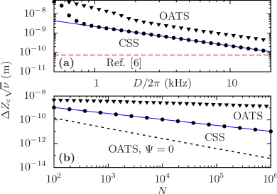
Figure 2: (Color online) Uncertainty in amplitude sensing with trapped ions for initial CSS vs OATS with maximal squeezing along $y$. (a) Dependence on $D$ for $N=100$ ions. (b) Dependence on $N$ for $D/2\pi=2$ kHz. Solid (blue) lines: analytical estimate for the initial CSS. Black dots: exact numerical optimization for the CSS. Dashed red line: uncertainty calculated in Ref. Gilmore et al. (2017) for the initial CSS. Black triangles: numerical optimization of the uncertainty from a cumulant expansion for the initial OATS. Dashed (black) line: initial OATS for $\Psi=0$ within the same approach. Parameters: $\omega_{z}/2\pi=1.57$ MHz, $U\delta k=40\times 10^{-24}$ N, $M=1.50\times 10^{-26}$ kg (from Ref. Gilmore et al. (2017)), and $\overline{n}=12.8$ resulting from a temperature of $1$ mK Sawyer et al. (2012).

Substituting the expressions of $y_{0}(t)$, $\chi(t)$ and $\Psi(t)$ into Eq. (7) gives $\Delta b(t)$ for an initial CSS. Within the regime described above, we find numerically that $t_{\mathrm{opt}}$ occurs for $Dt_{\mathrm{opt}}\gg 1$. For such long times, $\Psi(t)$ grows linearly with $t$, while $\chi(t)$ oscillates and remains bounded by $\chi(t)\leq 8(g/D)^{2}(\overline{n}+1/2)\ll\Psi(t)$, so that $\Psi(t)$ provides the dominant source of uncertainty. We then approximate $\chi(t)\simeq 0$ and expand the numerator and denominator of Eq. (7) at sixth- and zeroth-order in $\Psi(t)$, respectively, neglecting terms oscillating at $D$. To compare with Ref. Gilmore et al. (2017), we optimize the single-shot detection time, considering a fixed $\nu$, and find the optimal uncertainty $\Delta Z_{\mathrm{c}}\simeq{U\delta k}/[2{\sqrt{\nu}\,M\omega_{z}|D|N^{1/2}}].$ This uncertainty is plotted in Fig. 2 (solid blue lines), and shown to agree with an exact numerical optimization of Eq. (7) (black dots) for sufficiently large $D$ and $N$. Fig. 2(a) clearly shows that driving near resonance with $\omega_{z}$ causes $\Delta Z_{\mathrm{c}}$ to be orders of magnitude larger than estimated Gilmore et al. (2017) by neglecting correlated quantum noise (dashed red line).

Finally, we evaluate the uncertainty in amplitude sensing with an initial OATS. Taking initial values of $\beta$ and $\theta$ that minimize initial uncertainty along $y$, we numerically optimize $t_{\mathrm{opt}}$, using again a truncated cumulant expansion over the system. The black triangles in Fig. 2 show that rather than improving precision, this initial OATS leads to an uncertainty that is larger and suppressed more slowly with $N$ than for an initial CSS (a numerical fit gives $\Delta b\propto N^{-1/6}$). Thus, not only does this correlated quantum noise prevent the realization of the superclassical scaling $\Delta b\propto N^{-5/6}$ that would arise for $\Psi=0$ (dashed black line in Fig. 2(b)); but, in fact, the collective-spin state becomes “anti-squeezed” along the $y$ axis, making the scaling even worse than the SQL.

Discussion.— Interestingly, for collective noise as we consider here, the reduced state of the system can be written as $\rho_{\mathrm{S}}(t)=U_{\Psi}(t)(\left.\rho_{\mathrm{S}}(t)\right|_{\Psi=0})U_{\Psi}^{\dagger}(t)$, with $U_{\Psi}(t)\equiv\exp[-i\Psi(t)J_{z}^{2}]$ Nex . The quantum Fisher information being invariant under unitary transformations that do not depend on $b$ Braunstein et al. (1996), there always exists an optimal measurement that cancels the effect of $\Psi(t)$ in principle. However, not only is this measurement highly non-local in general, but it requires precise knowledge of $\Psi(t)$. This makes it far more challenging from an implementation standpoint.

In summary, we showed that spatio-temporally correlated quantum noise with frequency asymmetric spectra can generate unwanted entanglement of the sensing system that hinders superclassical precision scaling in Ramsey interferometry. Beside amplitude sensing with trapped ions, such noise sources arise naturally in a variety of other platforms – notably, superconducting qubits non ; Rigetti et al. (2012), nitrogen-vacancy centers Astner et al. (2017), or spin qubits in semiconductors Mi et al. (2018), in which qubit coupling to a common microwave cavity yields correlated photon shot noise. Our result is also directly relevant to ultrasensitive magnetometry and atomic clocks, as both fields are moving toward larger ensembles of entangled probes to reduce uncertainty below the shot-noise limit mag ; clo . This highlights the need for accurate characterization of quantum noise Paz-Silva et al. (2017), which may allow for counteracting unwanted entanglement through appropriate initialization, measurement, or dynamical control Paz-Silva et al. (2016).

It is a pleasure to thank Sandeep Mavadia and Jun Ye for useful discussions. F. B. acknowledges support from the Fonds de Recherche du Québec – Nature et Technologies. Partial support from the the US Army Research Office under Contract W911NF-12-R-0012 is also gratefully acknowledged.

References

- (1) V. Giovannetti, S. Lloyd, and L. Maccone, Phys. Rev. Lett. 96, 010401 (2006); C. L. Degen, F. Reinhard, and P. Cappellaro, Rev. Mod. Phys. 89, 035002 (2017).
- Bollinger et al. (1996) J. J. Bollinger, W. M. Itano, D. J. Wineland, and D. J. Heinzen, Phys. Rev. A 54, R4649 (1996).
- (3) J. A. Jones, S. D. Karlen, J. Fitzsimons, A. Ardavan, S. C. Benjamin, G. A. D. Briggs, and J. J. Morton, Science 324, 1166 (2009); R. J. Sewell, M. Koschorreck, M. Napolitano, B. Dubost, N. Behbood, and M. W. Mitchell, Phys. Rev. Lett. 109, 253605 (2012).
- Stace (2010) T. M. Stace, Phys. Rev. A 82, 011611 (2010).
- Biercuk et al. (2010) M. J. Biercuk, H. Uys, J. W. Britton, A. P. VanDevender, and J. J. Bollinger, Nat. Nanotechnol. 5, 646 (2010).
- Gilmore et al. (2017) K. A. Gilmore, J. G. Bohnet, B. C. Sawyer, J. W. Britton, and J. J. Bollinger, Phys. Rev. Lett. 118, 263602 (2017).
- Grote et al. (2013) H. Grote, K. Danzmann, K. L. Dooley, R. Schnabel, J. Slutsky, and H. Vahlbruch, Phys. Rev. Lett. 110, 181101 (2013).
- (8) I. D. Leroux, M. H. Schleier-Smith, and V. Vuletić, Phys. Rev. Lett. 104, 073602 (2010); M. H. Schleier-Smith, I. D. Leroux, and V. Vuletić, ibid. 104, 073604 (2010).
- Taylor and Bowen (2016) M. A. Taylor and W. P. Bowen, Phys. Rep. 615, 1 (2016).
- (10) S. F. Huelga, C. Macchiavello, T. Pellizzari, A. K. Ekert, M. B. Plenio, and J. I. Cirac, Phys. Rev. Lett. 79, 3865 (1997); B. M. Escher, R. L. de Matos Filho, and L. Davidovich, Nat. Phys. 7, 406 (2011); R. Demkowicz-Dobrzański, J. Kolodyński, and M. Guţǎ, Nat. Commun. 3, 1063 (2012).
- Chin et al. (2012) A. W. Chin, S. F. Huelga, and M. B. Plenio, Phys. Rev. Lett. 109, 233601 (2012).
- (12) Y. Matsuzaki, S. C. Benjamin, and J. Fitzsimons, Phys. Rev. A 84, 012103 (2011); A. Smirne, J. Kolodyński, S. F. Huelga, and R. Demkowicz-Dobrzański, Phys. Rev. Lett. 116, 120801 (2016).
- Dorner (2012) U. Dorner, New J. Phys. 14, 043011 (2012).
- Jeske et al. (2014) J. Jeske, J. H. Cole, and S. F. Huelga, New J. Phys. 16, 073039 (2014).
- Layden and Cappellaro (2018) D. Layden and P. Cappellaro, npj Quantum Inf. 4, 30 (2018).
- Szańkowski et al. (2014) P. Szańkowski, M. Trippenbach, and J. Chwedeńczuk, Phys. Rev. A 90, 063619 (2014).
- Bylander et al. (2011) J. Bylander, S. Gustavsson, F. Yan, F. Yoshihara, K. Harrabi, G. Fitch, D. Cory, Y. Nakamura, J. S. Tsai, and W. D. Oliver, Nat. Phys. 7, 565 (2011).
- Álvarez and Suter (2011) G. A. Álvarez and D. Suter, Phys. Rev. Lett. 107, 230501 (2011).
- Muhonen et al. (2014) J. T. Muhonen, J. P. Dehollain, A. Laucht, F. E. Hudson, T. Sekiguchi, K. M. Itoh, D. N. Jamieson, J. C. McCallum, A. S. Dzurak, and A. Morello, Nat. Nanotechnol. 9, 986 (2014).
- Malinowski et al. (2017) F. K. Malinowski, F. Martins, L. Cywiński, M. S. Rudner, P. D. Nissen, S. Fallahi, G. C. Gardner, M. J. Manfra, C. M. Marcus, and F. Kuemmeth, Phys. Rev. Lett. 118, 177702 (2017).
- Wang et al. (2017) Y. Wang, M. Um, J. Zhang, S. An, M. Lyu, J.-N. Zhang, L.-M. Duan, D. Yum, and K. Kim, Nat. Photonics 11, 646 (2017).
- Frey et al. (2017) V. M. Frey, S. Mavadia, L. M. Norris, W. Ferranti, D. Lucarelli, L. Viola, and M. J. Biercuk, Nat. Commun. 8, 2189 (2017).
- Chan et al. (2018) K. W. Chan, W. Huang, C. H. Yang, J. C. C. Hwang, B. Hensen, T. Tanttu, F. E. Hudson, K. M. Itoh, A. Laucht, A. Morello, and A. S. Dzurak, arXiv:1803.01609 (2018).
- Monz et al. (2011) T. Monz, P. Schindler, J. T. Barreiro, M. Chwalla, D. Nigg, W. A. Coish, M. Harlander, W. Hänsel, M. Hennrich, and R. Blatt, Phys. Rev. Lett. 106, 130506 (2011).
- (25) C. M. Quintana, Y. Chen, D. Sank, A. G. Petukhov, T. C. White, D. Kafri, B. Chiaro, A. Megrant, R. Barends, B. Campbell, et al., Phys. Rev. Lett. 118, 057702 (2017); F. Yan, D. Campbell, P. Krantz, M. Kjaergaard, D. Kim, J. L. Yoder, D. Hover, A. Sears, A. J. Kerman, T. P. Orlando et al., ibid. 120, 260504 (2018).
- Clerk et al. (2010) A. A. Clerk, M. H. Devoret, S. M. Girvin, F. Marquardt, and R. J. Schoelkopf, Rev. Mod. Phys. 82, 1155 (2010).
- Paz-Silva et al. (2017) G. A. Paz-Silva, L. M. Norris, and L. Viola, Phys. Rev. A 95, 022121 (2017).
- Bohnet et al. (2016) J. G. Bohnet, B. C. Sawyer, J. W. Britton, M. L. Wall, A. M. Rey, M. Foss-Feig, and J. J. Bollinger, Science 352, 1297 (2016).
- (29) J. Hu, W. Chen, Z. Vendeiro, A. Urvoy, B. Braverman, and V. Vuletić, Phys. Rev. A 96, 050301 (2017); B. Braverman, A. Kawasaki, and V. Vuletić, arXiv:1806.02161.
- Sawyer et al. (2012) B. C. Sawyer, J. W. Britton, A. C. Keith, C. C. J. Wang, J. K. Freericks, H. Uys, M. J. Biercuk, and J. J. Bollinger, Phys. Rev. Lett. 108, 213003 (2012).
- Rigetti et al. (2012) C. Rigetti, J. M. Gambetta, S. Poletto, B. L. T. Plourde, J. M. Chow, A. D. Córcoles, J. A. Smolin, S. T. Merkel, J. R. Rozen, G. A. Keefe, M. B. Rothwell, M. B. Ketchen, and M. Steffen, Phys. Rev. B 86, 100506 (2012).
- Paz-Silva and Viola (2014) G. A. Paz-Silva and L. Viola, Phys. Rev. Lett. 113, 250501 (2014).
- Paz-Silva et al. (2016) G. A. Paz-Silva, S.-W. Lee, T. J. Green, and L. Viola, New J. Phys. 18, 073020 (2016).
- Kitagawa and Ueda (1993) M. Kitagawa and M. Ueda, Phys. Rev. A 47, 5138 (1993).
- Brask et al. (2015) J. B. Brask, R. Chaves, and J. Kołodyński, Phys. Rev. X 5, 031010 (2015).
- Ma et al. (2011) J. Ma, X. Wang, C. Sun, and F. Nori, Phys. Rep. 509, 89 (2011).
- Wineland et al. (1994) D. J. Wineland, J. J. Bollinger, W. M. Itano, and D. J. Heinzen, Phys. Rev. A 50, 67 (1994).
- (38) See Supplemental Materials for a derivation of assuming an initial CSS or OATS, for a description of numerical calculations assuming collective noise, and for a derivation of the Hamiltonian used to describe amplitude sensing with trapped ions.
- (39) F. Beaudoin, L. M. Norris, and L. Viola, in preparation.
- (40) Though implies non-commuting (quantum) noise, note that the converse need not be true: for instance, for -correlated (white) quantum noise.
- Haase et al. (2018) J. F. Haase, A. Smirne, J. Kołodyński, R. Demkowicz-Dobrzański, and S. F. Huelga, New J. Phys. 20, 053009 (2018).
- Fröwis et al. (2014) F. Fröwis, M. Skotiniotis, B. Kraus, and W. Dür, New J. Phys. 16, 083010 (2014).
- Braunstein et al. (1996) S. L. Braunstein, C. M. Caves, and G. J. Milburn, Ann. Phys. (N. Y.) 247, 135 (1996).
- Astner et al. (2017) T. Astner, S. Nevlacsil, N. Peterschofsky, A. Angerer, S. Rotter, S. Putz, J. Schmiedmayer, and J. Majer, Phys. Rev. Lett. 118, 140502 (2017).
- Mi et al. (2018) X. Mi, M. Benito, S. Putz, D. M. Zajac, J. M. Taylor, G. Burkard, and J. R. Petta, Nature 555, 599 (2018).