Spherical cosmological models: an alternative cosmology
Abstract
The properties of universes are explored that are entirely in the interior of black holes in another universe, a ‘mother universe’. It is argued that these models offer a paradigm that may shed a new light on old cosmological problems. The geometry of such a universe is discussed including how it would appear to the observer. The Hubble parameter is direction dependent, but it is argued that the interpretation of any such dependence will be hard to separate from local inhomogeneities. The models do not originate from a big bang, but rather from an initial collapse and subsequent infall, that started probably a very long time ago, presumably much earlier than the accepted age of the universe. The relation to the concordance model is discussed and it is shown that a lot of the existing theory can be taken over into the proposed models. The universe has an edge, which is an ordinary spherical surface in 3 dimensions. That sphere acts as a gravitational mirror as seen from inside the universe, but it does not mirror redshift. The same object can thus be seen in direct sight and in reflection, although with different redshifts, different ages and different aspect angles. The models do not need dark energy, but they need dark matter, of course. Since the models are closed and neutrino’s are nowadays believed to have mass, neutrino’s can be reconsidered as candidates for the dark matter. As a bonus result from this paradigm, mass ejection from black holes is shown to be possible, which links that process to the controversial anomalous galaxy redshifts. Finally, we show that gravitational mass and inertial mass are proportional, and that the inertial acceleration scales as , with a characteristic length scale of the universe.
1 Introduction
It is well-known that a closed universe with a Robertson-Walker metric oscillates from the big bang to a maximum expansion state and back to the big crunch. At the maximum expansion state the radius of the universe equals its Schwarzschild radius , with the mass of the universe, the gravitational constant and the velocity of light.111See also subsection 2.1 for the definition of , and subsection 6.1. This suggests that one may explore universes that are the interiors of black holes. To this idea can be added that tidal forces generated by a spherical mass distribution scale as , with the distance to the center of the distribution. This result holds for the Schwarzschild metric as well ([1] 1973) in a local geodetic frame (freely infalling observer). Since the Schwarzschild radius scales with , it follows that at that radius the tidal forces for an infalling observer scale as . Hence these tidal forces are negligible for a very massive black hole.222This fact is of no particular importance for this paper, but is mentioned here because that idea germinated the paper. One is used to think of black holes as fierce things that destroy everything that pass the event horizon. Very massive black holes, on the contrary, offer a gentle, but irreversible, welcome. Of course, at the center of such a thing there waits disaster, but what if, as suggested above, inside the black hole there would be a distributed mass distribution and not a point mass? The density of such a distributed mass distribution with a constant mass density also scales as , hence could also be very small. The infalling observer would then simply enter a new part of spacetime, with the only consequence that he/she would never be able to leave it again. Such a thing could be called a universe, and it is the purpose of this paper to show that it actually is a universe much in the same sense as classical cosmology defines it.
In this paradigm, it comes natural to consider a 3D universe as embedded in another 3D universe. Since we will show that it can be the interior of a (spherical) black hole, we will adopt spherical symmetry. It is useful to make clear, from the outset, what the geometrical difference is between the universes in this paper and the standard Robertson-Walker (RW) universes. To that end, it helps to reduce the dimension by one, and consider 2D universes. A 2D RW universe is confined to the surface of a sphere, which is embedded in 3-space. In this paper, a 2D universe with positive curvature everywhere is the interior of a circle, though the surface inside the circle need not be flat. These universes therefore have a center (a point) and a boundary (a circle). Likewise, the 3D the universes we consider here have a center (a point) and a boundary (the surface of a sphere).
As for the center, we can characterize it in an ideal, perfectly ordered universe, which we will call a synchronous universe333According to this paper’s definition of synchronous, the RW models are synchronous. The characterizations of the center such as given here, are generally valid though and do not depend on synchronicity.. It is the only place were a material particle can stay put and not partake in the expansion or contraction. In reality, collisions during the contraction phase will give some momentum to any structure formed, and hence all matter will have velocities with effects that add to the effects of the expansion or contraction.444The wording here is unusually convoluted, since we will argue that the term ’comoving velocity’ is somewhat of a misnomer. In the same ideal world we will show that the center is the only place where the Hubble parameter is the same in all directions, but we will argue that current observations are not good enough to disentangle local anisotropies from the effects of sphericity, let alone that we would, at present, have a clue where we would be located in such a universe.
We will devote considerable attention to the boundary. Suffice here to state that also at the boundary space-time is locally 4D Lorentzian in all directions, as it is everywhere, since we will show that at the boundary the singularity in the radial coefficient of the metric (this is one of the characterizations of the boundary) can be transformed away.
In this paper we cannot exclude the now obsolete assumption that the universe could have gone through (many) cyclic phases of expansion and contraction, though we will try to define these contractions carefully and we will not need to assume any particularly neat periodic, nor global, behaviour. During contractions, the space time forced (or facilitated) structure formation, up to the merging of black holes and accretion of matter on them. The resulting dramatic increase in gravitational binding energy, together with increasingly intense background radiation, caused an immense radiation field, which therefore is a necessary companion of the next big bang, or rather, the next—relatively quiet—expansion phase. However, we will not, and need not, assume that a big crunch goes all the way to ”the point”; a condensed state, possibly with multiple centres in non-synchronous evolution, suffices.
The spherical symmetry (or possible more complex geometries for which spherical symmetry is but the simplest of all models) needs to be reconciled with the isotropy of the Cosmic Microwave Background (CMB). While in standard cosmology inflation is one of the mechanisms to obtain isotropy, acting from the inside out, we will argue that isotropy can also come about by the mixing that the phases of contraction imply, more in particular during the dense phases. This mixing acts, so to speak, from the outside inwards. Hence the universes in this paper are, by design, homogeneously filled with photons (which happen to be microwave photons in the current state of the universe). Of course, some riddles can be present, but unlike in standard cosmology these riddles are probably not particularly informative on the history of the universe.
Observations don’t seem to indicate that pressure is an important player, and therefore we can suffice with considering pressureless (dusty) universes.
This paper is best read by first jumping to the summary.
2 The model
2.1 Definitions and general principles
Spherically symmetrical and pressureless solutions of the Einstein equations have been studied extensively in the past. For a comprehensive overview of the available material in the context of all kinds of cosmological settings, the book by Krasinski ([2]) is very instructive. According to Krazinsky, these models were (re)discovered at least 20 times. He calls them L-T models, after the first discoverers Lemaître ([3]) and Tolman ([4]). In this paper, we start from the paper by Bondi ([5]), and adopt his notations for the metric:
| (2.1) |
with
| (2.2) |
the metric on the 2-sphere and
| (2.3) |
We use for the partial derivative with respect to . We choose and .
The 4-metric (2.1) is the Gaussian extension (see, e.g. [6]) to a fourth (time) dimension of the (spatial) 3-metric
| (2.4) |
with parameter . This extension is constructed along geodesics in the fourth dimension for which is the arc length and that pass through .
The time coordinate
| (2.5) |
has the dimension of a length and is the proper time for all particles with (geodetic) world lines , with , and constants. It is therefore a cosmic time that all such observers can agree on. These world lines also define the term ’comoving observers’.
In order to make the distinction clear between a time (with the dimension of time) and the time coordinate with the dimension of a length, we write the former in plain text font, and italicize the latter, as already indicated in (2.5). We will express time t in units of 10 Ga. If we adopt as the unit of length 3.066 Gpc, the velocity of light equals unity, and therefore, and t have the same numerical value.
We will sometimes refer to the Cartesian associated to the polar , and this we will do in the usual way: corresponds to the -axis, and the positive -axis is given by . Contrary to the usual convention however, we will construct space by rotating meridional planes (i.e. planes through the -axis with constant longitude ) over the angle , with in the interval . In every meridional plane the polar angle is then defined in the interval . This choice has the advantage that any meridional plane is fine to stage the motion along geodesics (which is plane motion), while in the standard convention this is only practical in the equatorial plane .555This choice implies a discontinuity in the orientation in the meridional plane and , but this is no inconvenience for this paper.
The radial coordinate , the dimension of which is actually undetermined and can (must) therefore be taken as dimensionless, has no direct quantitative relevance for radial distance. All points with the same we call a comoving shell, and accordingly we call the ”shell label”. The comoving shells are the reference spacetime surfaces that define the evolution of the universe. We can thus think of as the label that every comoving shell carries with it, and that can be read, by some unspecified means, by any traveler passing by. The shells can also be thought of as the rungs of a (growing or shrinking) ladder. The rungs have a unique label . A comoving observer stands on a rung, a traveler “climbs” or “descends” the ladder. The actual distance between the rungs is determined at all times by the metric (2.1), and equals .
The function , on the other hand, has a geometrical interpretation, in the sense that (a) it has the dimension of a length and (b) an elementary distance perpendicular to the direction of the origin (which we will call henceforth a tangential distance along a tangential direction) is measured by the familiar (here in a meridional plane). Because of this geometrical property and the fact that the surface of a shell at time equals , we will call a ”radius”. A shell with radius is interior to a shell with radius if . In that case shell is exterior to shell
The condition means that does play its role as a qualitative radial marker, in the sense that, at any time, the order relations in both and are consistent with the relations ”interior to” and ”exterior to” for comoving shells, if that was the case at the start (in time) of the validity of the model (i.e. the initial conditions). This we will assume.
The dimensionless function is arbitrary except for the obvious constraint and some integrability conditions (see later); we call it the energy function.666The reader may notice that in this paper sometimes notations are used that do not conform with standard texts or practices. This is in order to avoid notational conflicts with other parts of the paper. It is significant that it does not depend on . Hence, we restrict our shell labels to any strictly monotonic non-singular time-independent function of a particular chosen radial coordinate. Using for the ordinary derivative with respect to , this means . As a consequence, the class of valid shell labels leaves independent of time. Note in particular that if belongs to this class, we could adopt as the radial coordinate.
The local Lorentzian dust density is determined by (Bondi [5], Krasinski [2])
| (2.6) |
with another arbitrary function with the dimension of a length, whose physical meaning will be clarified later. The function would be equal to times the total mass inside shell if space were Euclidean. Expressed in our units of length and time, we find
| (2.7) |
and we adopt as our unit of mass density, which is basically equal to the standard critical density of the universe
| (2.8) |
assuming for the current Hubble parameter
| (2.9) |
Note that will always appear in combination with as the product with the dimension of the inverse square of a length, since has the dimension of a length divided by a mass. It follows thus from our choice of the units (time, length and mass density) and (2.7) that in numerical value
| (2.10) |
The volume element of the 3D metric equals
| (2.11) |
Note that the notation is actually shorthand for , since is defined in the interval .
The cumulative mass function, which is the total mass interior to a comoving shell with label thus reads
| (2.12) |
and it is, according to the second equation in (2.12), obtained via (2.6), also independent of the time. That second equation can be readily inverted:
| (2.13) |
In our units, we find for the first equation of (2.12)
| (2.14) |
The constancy in time of and means that the constituent matter of the universe stays put on their shells, and hence, we can refer to that matter as comoving matter.
It follows from (2.6) that
| (2.15) |
We are now in the position to identify the shell exterior to which there is no comoving matter. That shell we call the outer boundary and its shell label we denote by . Hence
| (2.16) |
As is obvious from (2.6) and (2.11), the occurrence of is special. We will assume it occurs at at all times, which therefore defines the inner boundary of the model, which we call the center, and we set there.777This is of course what is common practice in polar coordinates. In some strict mathematical sense, ’the origin’, defined as the locus where , is not part of the space that polar coordinates cover. The origin is part of the manifold, though, since an appropriate transformation (Cartesian coordinates) can eliminate the singularity. We will see in section 6.4 that the only shell with where can be is the boundary .
If at some shell with label and at some time while , the mass density reaches a singularity according to (2.6).888Note that this condition is independent of the choice of the shell label. This means that shells are colliding there, and a collision therefore marks the end of the validity of the metric. The geometrical model (i.e. the metric) is therefore only valid for these parts of spacetime that are either fully expanding or collapsing without any shell crossings.999Usually this is interpreted as consistent with the fact that the model is pressureless, since shells bumping into each other would create pressures. In a cosmological context this is less so the case, since we observe that colliding matter forms gravitationally bound structures such as (clusters of) galaxies and black holes, which do not necessarily increase the cosmic pressure significantly. The term “shell crossing” was introduced by Hellaby & Lake in [7]. Our use of the term “shell collision” refers to the point expressed in this paragraph: there is no geometrical model anymore at a shell collision, lest one introduces new physics and resolves the singularity.
It is also possible that for some shell . We will show in section 6.4 that for the models we consider an appropriate transformation can eliminate this singularity, which must if the spacetime is to be Lorentzian. Hence that shell is also part of the manifold.
We will assume that, at all times for which the model is valid
| (2.17) |
Hence, we call the first inequality of (2.17) the no-collision condition, since it is extremely unlikely that, in view of the presence of collapse phases, over a range in , except possibly around the center. The second inequality between brackets is an assumption. Should for some and , we will assume that the singularity can be transformed away by another choice of the shell label.101010This is only possible in the case that is separable in and . An example would be a singularity of the type The singularity can be trivially removed by adopting a new shell label .
The spacetime in which the metric (2.1) is valid is the direct product of (a) all shells with comoving matter () for which the no-collision condition (2.17) is valid and (b) the time interval
| (2.18) |
Equation (2.18) defines the symbol and means that at some shells will be colliding. The lower bound of the interval is as yet unspecified.
In case we will have occasion to use the normalized shell label
| (2.19) |
We denote
| (2.20) |
and assume that is finite for finite .
If we integrate (2.6) with an Euclidean volume element, we obtain
| (2.21) |
yielding an ’Euclidean total mass’ for that is proportional to rather than to the total mass of the universe
| (2.22) |
The right hand side equals and is very reminiscent of the expression for the Schwarzschild radius. On these grounds could actually be interpreted as the mass of the black hole as experienced by an observer ’outside’ the universe (but see also section 4 for a proof of this assertion). On the other hand, nothing more specific can be stated between and than what would follow from relations (2.12) or (2.13), since is (still) an arbitrary function.
2.2 The evolution equation
The time evolution of and is governed by (Bondi [5], Krasinski [2])
| (2.23) |
with the cosmological constant. It is actually already an integration of the equation
| (2.24) |
As is well known, the structure of these equations is essentially the same as the Newtonian analogues, apart from the presence of the cosmological constant. More particular differences include an overall factor of and the quantity , since in the Newtonian case it would be , according to (2.13) and (2.6). Following Bondi ([5]) we call the effective gravitating mass function and hence the total effective gravitating mass.
We note in particular that the effective gravitating mass function does not explicitly enter the metric (2.1), but has only impact on the time evolution through equation (2.23). From the sign in front of in (2.23) we conclude that the Newtonian analogue of would be proportional to the negative of the total energy, and we will call the energy function. The non-Euclidean character of the model resides solely in the time dependence of , since if , a suitable radial shell marker transformation makes the metric (2.1) Lorentzian.
It is instructive to ponder the similarities and differences of the motion of the shells we consider here and the classical 2-body motion of celestial mechanics (barring the cosmological constant). In 2-body motion, the equations (2.23) or (2.24) describe the motion of 2 point masses on degenerate ellipses (i.e. straight lines). If we put the center of mass of the point masses in the origin and their linear orbits on the -axis, one point is moving on the positive -axis and the other on the negative -axis. They both reach their largest distance from the origin at the same time, and they collide (elastically) at the origin. The more common view is to place one of the point masses in the origin, and the other then oscillates on one side of the -axis, with periodic collisions. In this paper, the shells behave similarly in the sense that they oscillate from largest surface area to zero surface area, ideally back and forth. However, comoving observers will ’fly through’ the center when reaching it, and if they were infinitesimally small, they wouldn’t collide with anything.
The velocity in the 2-body motion is entirely determined by the magnitude of the participating masses and, say, the distance of greatest elongation (or velocity at infinity). This is no different from what we have here: all motion is ’simply’ due to gravitation. For shells with the same surface area, (a measure for) the expansion or contraction rate will be larger if the mass of the universe inside them is heavier.
This is the place to point out that the dimensionless is not (proportional to) the radial velocity of anything. Actually also here, as in the 2-body case, for if , and thus, if is sufficiently small, can be larger dan . While an infinite velocity is no problem in Newtonian dynamics, it clearly shows that here is not a material velocity: it is a measure for the change in tangential distance of 2 comoving points, or, technically more precise, it is proportional to the geodetic deviation of 2 neighbouring comoving points at the same .111111The ratio is the tangential Hubble parameter (see section 3.5). In this context this ratio can also be characterised as follows. Be the infinitesimal meridional angle subtended by the meridional tangential distance covered by a particle with meridional tangential velocity on shell at , with , during an infinitesimal time interval . At time this angle would be . The ratio of both angles equals for . Hence in an expanding universe a particle or photon progresses less far from an angular perspective at the origin than it would in an Euclidean universe. We note in particular that there is no limit on the magnitude of . We call the tangential stretch (or shrinkage) rate, and denote it by the dimensionless
| (2.25) |
We introduce this, at first sight somewhat pedantic, additional symbol for in order to remind us that is not a velocity. Hence the term ’comoving observer’ is in a strict sense a misnomer, and the term co-stretching or co-shrinking would be more appropriate. This paper adheres to the common terminology, though.
Clearly, we could also define a radial stretch rate , but this definition does not carry much added value for this paper.
As we will see in section 4, we will not adhere to the view that it is space that is expanding (created) or contracting (annihilated), but rather shells that are expanding or contracting in spacetime.
Returning to our ladder analogy, the distance between rungs is given by the Lorentzian
| (2.26) |
at constant (hence and we can label the rungs with instead of ). We clearly see the Schwarzschild term which makes larger with increasing , and therefore makes space more elliptic. The (longitudinal) stretching or shrinking rate of the rungs is proportional to . The larger that rate (in absolute value), the closer the rungs are to one another, which is thus the opposite effect as , making space more hyperbolic. This is somewhat reminiscent of a Lorentz contraction. Finally there is the role of the cosmological constant which is obvious from (2.26) but not very intuitive. All 3 effects combine in such a way as to make the radicand in (2.26) independent of time. The radial Lorentz distance of course isn’t, since it features the factor .
We conclude that the non-Euclidean character is very closely connected with the mass content and the kinematics. The only static model that is stable is the empty Euclidean space, with .121212The only other static model has , and as can be seen from (2.23) and (2.24). It is the one for which Einstein introduced the cosmological constant. The repulsive force of a positive exactly balances the attraction caused by the effective gravitating mass, but this delicate balance is, of course, unstable.
Finally, the no-collision condition (2.17) can always be realised for the initial conditions (at some cosmic time, to be discussed later), since shells can be ordered with respect to surface, and each shell can be given a label that preserves this order. An obvious choice would be
| (2.27) |
with only taking the numerical value of (and not its dimension).
3 The current expansion phase
3.1 Definitions
Since we will be concerned in this paper only with the fully expanding universe without collisions, we will suffice with ”simply” specifying and under certain conditions (see later), and subsequently solve the evolution equation (2.23) for .
The solutions of (2.23) are well known. They are found via an implicit form, as a function of that is, by the quadrature:
| (3.1) |
This expression introduces quite some functions. We start with defining
| (3.2) |
valid for all and (in a collision-free universe, that is), in contrast with the of equation (3.1) which is only valid for those and that realize the integral on the left hand side. We call the function the state of the shell with label at time . It is dimensionless. The quantity we call the phase of the shell , and is to be seen as an integration constant (as a function of ) in the solution of (2.23). The quantity is also called “bang time” for obvious reasons, but since we will assume that our universe actually does not realize the limit , this term is not very appropriate.
The radius is given by
| (3.3) |
with
| (3.4) |
We call the shell parameter of the shell with label . It has the dimension of a length. Next is
| (3.5) |
which we call the shell ’frequency’, with the dimension of a reciprocal length. The function
| (3.6) |
incorporates into the expression (3.1) and is dimensionless.
Still to be defined is . We distinguish 2 cases, which we call representations.
(a) The function is defined as a constant:
| (3.7) |
The third case applies when in a non-empty interval of (see appendix A.3 for the details).
(b) The function is the function:
| (3.8) |
and hence
| (3.9) |
Both representations (a) and (b) have their merits and drawbacks. For example, representation (a) cannot be used in the numerical calculations when at some , as can be seen from (3.4). On the other hand, representation (b) introduces additional and strictly spoken unnecessary -dependence in the function cyc. Obviously, in both representations, there remain only 2 independent functions: and , while the quadrature (3.1) introduces the independent phase function .
The energy function appears in the metric, and hence we must assume that it is sufficiently differentiable. Barring Dirac- behaviour in but allowing discontinuity, it follows from (2.12) that is continuous (not necessarily differentiable) and non strictly monotonously increasing. With (2.13), the same is true for the effective mass function . Since both functions and will need to be differentiated once in the orbit calculations, continuity for both functions suffices.131313If only this minimum requirement is met at a certain shell , one would need to account for this by stopping the integration at that shell with a certain set of (say, left) derivatives, and restarting it with a different set of (right) derivatives, causing a kind of refractive behaviour at that shell. For flux calculations we will also need the second derivatives of and , and thus continuity in their first derivatives. This means, with (2.6), that in that case must be continuous.
The effective mass function features the parameter , which we called the total effective mass. We can normalize , and define
| (3.10) |
Likewise, we can explicitly introduce a scaling in the shell parameter
| (3.11) |
and the shell frequency
| (3.12) |
Equation (3.1) determines implicitly the function , and it is discussed at length in appendix A. For and it is the familiar cycloidal function. The name ”” makes explicit reference to the family of cyclic solutions of (2.23), but is here taken to be more general, also allowing for the monotonously expanding solutions.
When , the total effective mass is a scaling parameter, both in space and . The scaling in space follows from the dependence of on , while the (inverse) scaling in follows from . When the proportionality is lost, since depends non trivially on which is also affected by the scaling.
In a globally expanding universes (i.e. all shells are expanding), we need only consider the branch of for which and thus . When has a maximum as a function of , we denote by the state at which that maximum is attained. The function is also discussed in appendix A. If present,
| (3.13) |
is the expression for the maximum radius that a shell with label can attain. We omitted explicit reference to the dependence of and on for clarity. The expression (3.13) defines , and is discussed in detail in appendix A.141414When and we have and .
As to the no-collision condition (2.17), it is hard to deduce any general statement as a condition that is relevant for because of the interdependence of the various functions appearing in (3.3). Hellaby & Lake [7] produced such conditions for the case , employing the particularly simple parametric equations for in that case. In practice, when considering a particular model, we will rather first ’simply’ verify (2.17) for all shells, and determine as indicated in connection with its definition (2.18).
From table 2 in appendix A we can deduce that if all shells will attain a maximum radius, irrespective of the sign of . On the contrary, if for shell , that shell is unbound, again irrespective of the sign of . When boundedness depends on the sign of . Unbound means that the expanding shell will expand forever, that is, for as long as it does not bump into another shell. An upper bound on the maximum time span of validity of the metric is the minimum of all
| (3.14) |
if bound shells are present.
3.2 The phase function
In order to interpret the phase function in (3.1), we recall that, in our paradigm, at the end of the latest collapse, the universe was probably in a compressed, hot and chaotic state with shells bumping into or overtaking each other. The subsequent rebound also surely created instances and places where the no-collision condition (2.17) was violated. Since the current state of the universe seems to indicate that no major collisions occurred since a long time, there must have been a moment when all shells were again partaking in the expansion and condition (2.17) was satisfied throughout. The origin of time in a valid model is therefore that moment at the earliest, and the model therefore starts with shells on radii
| (3.15) |
We will assume that the model is ”maximal in history”, which by definition means that the above equation at implies that the universe emerges at that time from a (temporarily last) collision of shells at some . All states are positive from that time on, and the global model is valid until, again, some shell bumps into another one. The phase function is implicitly determined by the initial condition (2.27) and the inversion of
| (3.16) |
We must keep in mind, though, that our origin of time only marks the start of the validity of the metric and may very well be considerably smaller than the age of the oldest (compact) structures as we know them now. In other words, if the oldest structures are 13 Gyr old (in our units ), then that does not necessarily mean that the universe as a whole has been expanding for the last 13 Gyr according to the rules of our model, i.e. without colliding shells. If we call ”the age of the universe” the duration of the validity of the model in the current expansion phase, as usually, we can very well consider values for this time span that are considerably shorter than 13 Gyr without a priori dealing with a model that is at variance with observations or generally accepted views. We should also keep in mind that the above defined non-collisionality is probably an (unnecessary) strong requirement from the physical point of view, but it is forced upon us because of the geometrical nature of a general relativistic cosmological model.
Lastly, but not in the least, a phase function that is increasing with increasing has the effect that the outer parts of the universe are more evolved than what the term could bring about, thereby effectively having an effect of acceleration, without having to invoke dark energy. This property has already been noticed and studied by Iguchi et.al. [8]. Since the observable properties of a universe are closely related to the paths of photons, we will have to defer the effects of the phase function to section 9, more in particular section 9.6.
3.3 The central region
It seems reasonable to assume that the mass density in the center tends to a constant, as a function of that is. In these conditions, integration of (2.6) leads to
| (3.17) |
The constancy of (as a function of ) is also consistent with the Newtonian limit (representation (a))
| (3.18) |
since must be proportional to . We recall however that is a dimensionless shell label, and therefore the factor in (3.18) has the dimension of a length and merely realises the one-to-one relation of shell labels and physical radii in the central regions. Using (3.3), we find
| (3.19) |
and, in view of (3.17):
| (3.20) |
with a constant with the dimension of a mass density, and
| (3.21) |
The second part is a consequence of the definition of in (3.5), which tends to the constant
| (3.22) |
and the last equality of (3.21) defines (dimension of length).
The energy function is defined in representation (a) as
| (3.23) |
and therefore tends quadratically to zero:
| (3.24) |
with
| (3.25) |
This is again consistent with the Newtonian limit.
3.4 Geometrical considerations
3.4.1 The Riemann scalar
The Riemann curvature scalar of (2.1) reads (Bondi [5])
| (3.26) |
with the Riemann curvature scalar of the 3-dimensional subspace (2.4):
| (3.27) |
We find, using (2.3),
| (3.28) |
Clearly, for , the universe has zero curvature.
The curvature tends towards the spatial constant in the center.
3.4.2 The nature of the curved space
It is customary when discussing curved 3-spaces with spherical symmetry to lower the dimension by suppressing one angular coordinate and to consider the nature of such a surface. Here we will consider a (non-Euclidean) meridional surface with a constant, and thus we will suppress the longitudinal angle. The essential differences of such a surface compared to a meridional plane in Euclidean space is that, (a) while in the Euclidean plane 2 neighboring points on radial orbits apart have to travel a (Lorentzian) radial distance in order to change their tangential distance by (independent of !), on the meridional surface this (Lorentzian) distance would become , and that (b) this distance depends on the shell .
As for the 3D universe, we can always (because of the symmetries) place the observer on the -axis by means of a 3D rotation. For not in the center , the direction towards would be a direction on the celestial globe, say, a celestial pole. In the 2D cut on which we placed the observer ( is arbitrary since is on the -axis) and to which we confined his/her view, this view translates into confinement to look along a great circle through , and thus a meridian. In that 1D sky, there is mirror symmetry as seen from with respect to the direction , because of the circular symmetry around . In the full 2D sky as seen as the projection of the real 3D universe, this translates into the property that for any observable function on the sky that is the projection of a 3D function that satisfies the spherical symmetry condition around , with right ascension and declination, , since the declination of an object is the angular distance from that object to . Put differently, the independence of reflects the rotational symmetry of the meridians through the -axis (the celestial poles), or the arbitrariness of the choice .
3.4.3 Embedding surfaces
We choose the 2D cut , i.e. the coordinate plane, and build on it a surface that bulges into the dimension. Because of the spherical symmetry in the plane this will be a surface of revolution that can be described by a function . On that surface we consider the coordinates .151515Note that is now also a coordinate, which means that is a parameter. This is possible because at any given time we can choose . We construct a surface in Euclidean 3-space () or Minkowski 3-space (), both built on the chosen Euclidean meridional plane with metric or :
| (3.30) |
expressed in cylindrical coordinates . We require that on that surface the metric equals the metric of the 2D cut:
| (3.31) |
This yields a surface of revolution around the -axis in Euclidean 3-space or Minkowski 3-space, with the property that the of the original metric is preserved, be it, of course, that for Minkowski space () the distance in a plane of constant is given by instead of the Euclidean for . That surface thus ’bulges out’ of the Euclidean meridional plane into an Euclidean 3-space or a Minkowski 3-space . This 3-space does not correspond to any reality however. It is simply the space we need to construct this isometric representation of the cut through the original space. We find
| (3.32) |
In a standard cosmology with uniform positive curvature the isometric representation is the surface of a sphere.161616We come back to this case in section 6.1. At this point it needs to be remarked that the embedding surface we consider here only bulge out on one side of the Euclidean plane (for an observer located at ), and are not continued ’below’ it, in contrast with the common picture in cosmology. For now, this can be best appreciated by considering the limit which is likewise not a ’double’ Euclidean plane. We return to this extensively later on.
3.5 Models that realise a given
3.5.1 Definitions
The Hubble parameter is defined for synchronous homogeneously filled universes (see section 6.1). We denote
| (3.33) |
where the plain text font for H and the partial derivative with respect to t (and not ) indicate that H has the dimension of a reciprocal time. The expression (3.33) reduces to the usual expression in the standard cosmological models. We call the quantity (3.33) the tangential Hubble parameter or simply Hubble parameter.171717In section 9.1 we will have occasion to define the radial Hubble parameter. See also the end of this section. In our units, , and we therefore redefine
| (3.34) |
expressed in inverse length. We denote
| (3.35) |
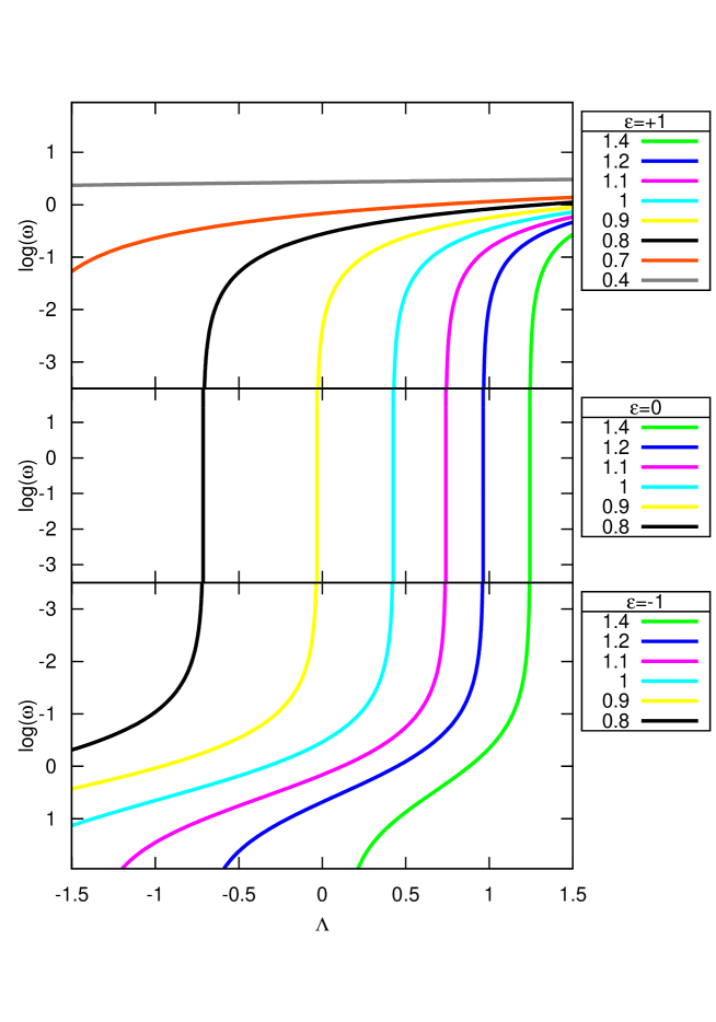
with and denoting a particular shell at a particular time. If and refer to our position and our epoch, we denote them by and . With as given by (2.9), equation (3.33) implies or, with equation (3.34) . Therefore, we can concentrate on models that realise somewhere, sometime. The rule-of-thumb conversion between and our units is easy: division by 100.
We can suffice in this section with representation (a), i.e. equal to , or .
3.5.2 Classification
In order to identify the models that realise a given somewhere, sometime, we need to solve equation (3.36) for .
We first consider the bound shells, i.e. the shells that reach a maximum . Since
| (3.38) |
it is obvious that if or . When , one can prove, with the material provided in appendix A, that if is bounded, since . Since for and monotonically for approaching rebound time ( in the notations of appendix A), there is a unique solution for and thus a unique state that realizes a particular when is bounded.
When is unbound, for (recall (3.6). Hence there is always a unique solution for finite when and or due to (3.38). For , unboundedness means that (see table 2). Equation (3.38) learns that has a minimum equal to at . Hence if and there are 2 solutions, one for and one for . This occurs therefore if . If only the one less than remains.
| Shell | Condition | Solutions |
|---|---|---|
| Bound | None | 1 |
| Unbound | 1 | |
| and | 2 | |
| and | 1 | |
| 0 |
3.5.3 Solutions
In the cases where there is a unique solution, which we denote by , the equation (3.36) which is to solve is similar to the one considered in appendix A. Denoting
| (3.39) |
we need to solve
| (3.40) |
This equation is already in the Cardano form, and we find readily
| (3.41) |
if or
| (3.42) |
otherwise. Equations (3.41), (3.42) and (A.1) define a function .
The integral (A.1) is always well-defined. This is obvious if is unbound, since the radicand in the denominator is never zero, by definition. If is bound, the inequality we have to verify is
| (3.43) |
This is easily done, since the above inequality and (3.40) transform into
| (3.44) |
This does not necessarily mean that there is a time where is realised however, since the value for may not lead to a positive because of a phase that is too large. Hence we can maximise the number of models that realise some given sometime, somewhere, by setting .
The function therefore defines a function , defined for through
| (3.45) |
When , and thus , expression (3.41) shows that . In that case it follows from (3.36) that
| (3.46) |
while, from equation (A.23),
| (3.47) |
Hence, under these conditions,
| (3.48) |
which is the behaviour of the Hubble parameter at very early times, and thus, for
| (3.49) |
Since scales inversely with the total effective mass, this is also the limit for large . This can be understood because the larger the less evolved a model is for a given time, and thus the more the relation (3.48), valid for small , is approached.
In the case when there are 2 solutions, which we denote by , we obtain
| (3.50) |
and
| (3.51) |
Which of the 2 is realized depends on the details of the particular universe considered.
3.5.4 On the radial Hubble parameter
The tangential Hubble parameter is the Hubble parameter that is measured in a tangential direction, i.e. in a plane perpendicular to the direction of the center of the universe. In section 9.1 we define the radial Hubble parameter as the Hubble parameter that is measured in the direction of the center (equation (9.10)). Clearly, because of the derivatives with respect to that are involved, we cannot make easily general statements such as the ones we obtained for the tangential Hubble parameter. E.g., for large and thus small , we can use the approximation
| (3.52) |
to obtain
| (3.53) | |||||
This little enlightening expression for a special case shows that general statements will be hard to formulate. In the limit however, it follows from (3.19) that , which means that if we choose shells sufficiently close to the center, the difference between and will never be an issue. Also, we will see in section 6.1 that in standard cosmologies and are constant functions, while . Hence in these cases .
3.6 Connection with standard notation
Equation (2.23) can be rewritten as
| (3.54) |
defining the familiar , en in terms of our notations. We omitted the dependence on and for clarity. In terms of the function cyc, we find, preserving the order of the terms in (3.54),
| (3.55) |
In the universes we consider the above functions depend on and , while in standard cosmologies they only depend on (see also later in section 6.1).
We know continue with a standard analysis in order to solve (2.23). We first multiply (3.54) with :
| (3.56) |
and transform this expression with the well-known relations181818We will see in section 6.1 that the in this paper is not what in many texts is called , the radius of the universe. Equations (3.57) remains valid though, because our definition of is the same as the standard one.
| (3.57) |
into
| (3.58) |
Integration yields, with ,
| (3.59) |
The above integral is equivalent with (3.1) or (A.1) upon transforming
| (3.60) |
taking account of the definition of in (3.4) and a shift of the origin, since in (3.1) the origin of time, which is the start of the validity of the metric, is left undefined, while here is the current epoch.
3.7 On the flatness problem
From the second term in (3.55) we see that at early times (the flatness problem). In our paradigm, this feature rather appears as a peculiarity of the decomposition in the ’s instead of something particularly fundamental that needs to be explained. This comes about because here we do not expect the expansion phase of the universe to start from a point, and any phase term would make this particular feature disappear. We will return to a discussion of the early times in section 5.2.
4 Beyond the mass distribution
In this section, we consider a finite matter distribution that finds itself in an era of universal expansion or contraction. Denoting
| (4.1) |
the radius
| (4.2) |
encloses all effective gravitating mass . If the matter distribution is embedded in empty space, beyond this physical radius we should find ourselves in the Schwarzschild- metric
| (4.3) |
If the coefficient
| (4.4) |
is positive (it need not be), then we can interpret as proportional to the familiar Schwarzschild- coordinate time ,
| (4.5) |
using the same convention as (2.5) and a measure for the total gravitating mass. That these assertions can be made follows from the classical theorem that a time dependent spherical mass distribution of constant total mass creates a gravitational field beyond its boundary that is the same as the field of a point mass with a mass equal to the total gravitating mass of the mass distribution. We will see shortly that it is correct to use the same symbol as it was defined in (2.20).
The coefficient has 1 or 2 positive roots . In the case of 1 root, the root is the Schwarzschild radius . In the case of 2 roots we denote the roots . The notation follows the notation of appendix B.1 and refers to the effective potential of a radial orbit. We now have to distinguish 2 different cases.
4.1 Particles can reach the space beyond the mass distribution
If for all the energy function , then there is no singularity in (2.1) and there is no (see also later). We are in the case of a dust ball. When calculating orbits, the transition from the inner metric (2.1) to the outer metric (4.3) and vice versa is done at the moment the particle passes the outermost shell at radius given by (4.2) with coordinates and coordinate velocity . The integration is stopped at that moment, and resumed after transforming coordinates and velocities to the Schwarzschild- metric. This can be done by noting that the universe metric at that point can be seen as an Novikov metric, and therefore the procedure outlined in appendix B.4 is applicable. The stationary Novikov observer is the comoving observer at . The velocity that this observer should be assigned to from the perspective of a stationary Schwarzschild- observer is therefore given by (B.26):
| (4.6) |
The sign of depends on whether we are in an expansion phase or a contraction phase . The effective potential is known since is known, and the normalized relativistic energy is known, by definition, as a characteristic of the dust ball in the Schwarzschild- world. We can subsequently perform the Lorentz transformation from the velocity of particle
| (4.7) |
in the local Lorentzian frame of the shell to the velocity in the local Lorentzian frame of the stationary Schwarzschild- observer with the inverse Lorentz transformation of (B.28). Finally we can pass on to
| (4.8) |
and coordinates at some (to be defined) time , and resume the orbit calculation in the Schwarzschild- frame.
For light, we also need to calculate the refraction angle, so that the wavelength change can be determined (subsection B.4).
All this occurs irrespective of the time evolution of the dust ball (oscillation, permanent expansion, or mixed forms), and without special consideration of expansion due to , since is common to both representations.
The procedure for a particle that falls into the dust ball from outside is similar (mutatis mutandis).
4.2 Particles remain confined inside the outermost massive shell at
4.2.1 The definition of a universe
In the case for some shell, we can take that shell to be , since the metric (2.1) is only defined for shells with comoving matter. If we assume that is finite (see table 2),
| (4.9) |
is the largest possible value of in the valid spacetime of the metric (2.1). Inserting this value for in
| (4.10) |
we recover the definition of as the root of introduced in appendix A, with given by (B.5), if and only if . This proves that the case of a universe from which nothing can escape, and therefore with an outer solution (4.3) which is a Schwarzschild- black hole, has and fills completely its allowed volume at maximum expansion. Hence, the Schwarzschild radius , solution of (4.10), is also given by
| (4.11) |
and at all other times the maximum radius . Spacetime with has the signature of an inner Schwarzschild- metric.
4.2.2 Infalling particles
We consider infalling particles from outside the black hole. Since we need to cross the horizon, we adopt the Novikov frame (appendix B, and more in particular section B.4).
Parallel to the events in the mother universe, the universe inside the black hole is also evolving. Any particle (massive or a photon) that ventures from outside inside must follow a course with decreasing (see also section B.3), and will eventually reach the edge of the universe inside , at as given by (4.2), a cosmic time that is indeterminate, and at in the Novikov frame. From that time on we can, and must, consider the orbit in the universe.
Novikov coordinates and cosmic coordinates are strictly disjunct, because everything in the Novikov frame is traveling with decreasing while the boundary of the universe on the contrary is expanding and therefore cannot be described in the ingoing Novikov metric: the boundary behaves as a comoving shell in an outgoing Novikov metric. Therefore we need a metric that encompasses both metrics, and the obvious choice is the inner Schwarzschild- metric ()
| (4.14) |
As is well known, the roles of and have switched. An infinitesimal time interval is given by while a radial length is . The Lorentzian radial velocity in the inner Schwarzschild- metric therefore is
| (4.15) |
The second equation is relevant for Novikov shells in their coordinates . Using (B.2), we obtain191919In section B.1 it is quite irrelevant whether we deal with the inner or the outer Schwarzschild- metric: the analysis is valid outside and inside
| (4.16) |
The boundary shell of the universe follows the outgoing Novikov orbit (4.2), which we now can write as
| (4.17) |
This boundary will eventually touch , and since it is an outgoing Novikov shell turning into an infalling one, it has in the Novikov swarm, with the appropriate . We thus find that the boundary of the universe has zero Lorentzian radial velocity in the inner Schwarzschild- metric. This is in concordance with the results of section 7.2.
The other infalling Novikov shells on the contrary have . The expression for the radial velocity (B.3) in the outer Schwarzschild- metric now reads in the inner Schwarzschild- metric as
| (4.18) |
with the positive sign, since in the inner Schwarzschild- metric has the character of a time, and is therefore a relation between 2 times, which is always positive (and irrespective of the circumstance that the universe is expanding or contracting). Note also that, since , there is no a priori limit on the magnitude of . This is no problem because is not a velocity.
Insertion of (B.3) in (4.16) yields
| (4.19) |
The effective potential , and thus , as should.202020Note that standard treatises denote our as , which is clearly not appropriate inside the Schwarzschild radius.
The transition from Novikov coordinates to cosmic coordinates is similar to the transformation explained in section B.4. The infalling observer at with coordinate velocity encounters at Novikov time the boundary shell , which happens to be at cosmic time . The relation between and is undetermined. The particle coordinate velocity transforms into the local Lorentzian Novikov frame velocity according to
| (4.20) |
At the boundary of the universe, the Novikov frame has radial velocity given by (4.19). The Lorentz transformation of subsection B.4 then yields , with the local Lorentzian radial velocity component that will be needed in section 8 (it is defined in (8.16)) in order to integrate the orbit at and at further in the universe.
For light, the procedure is the same, but we also need to calculate the refraction angle in order to determine the wavelength change (subsection B.4).
We also note that inspection of (4.20) learns that, since can be positive, an infalling particle or photon can enter the universe with an outward velocity!
5 The universe before the present expansion phase
5.1 The latest collapse and structure formation
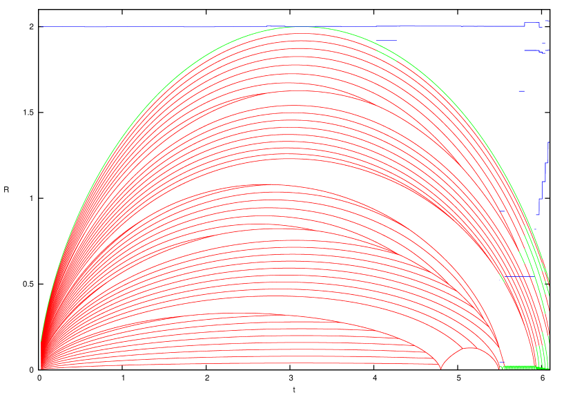
In our paradigm it would be grotesque to assume that the universe somehow originated from a point, with at the time of ’creation’ and , . We must assume that the universe has gone through at least one collapse, and therefore it is instructive to outline how such a collapse could be modeled.
Since we are concerned here with the latest collapse, we will assume that the universe is cold enough, so that the matter is localized on a number of thin shells with surface density , . Allowing for the spherical symmetry, this is certainly not contrary to the observations, since we can think of the shells as a kind of galaxy clusters, with one dimension that is small on a cosmological scale. We order them according to increasing and the ’s are thus the shell labels. The clusters have mass and tangential stretch rate .
In order to establish the initial state of the universe, given the initial conditions , and , we first recast the relation (2.6) into a difference equation
| (5.1) |
This choice of the indices ensures that the gravitating mass on shell has no impact on the dynamics of shell . Likewise, the cumulative mass (2.12) gives rise to
| (5.2) |
The energy at shell reads:
| (5.3) |
From (5.2) we calculate in a recursive way since the are given, and from (5.3) and the known and we find . The recursive scheme starts with , and is an (optional) mass in the center. Note that the solution does not depend on the sign of , reminding us of the same feature in the Lorentz contraction. This also shows that the scheme we have outlined is also valid for an expanding universe, or even for a mixed universe with parts in collapse and parts in expansion.
As for the metric, we may set . We define
| (5.4) |
In contrast to (5.4), the energy function is undefined as long as we do not specify the tangential stretch rate for . It is useful to think of the space between shells as being filled with a dynamically unimportant ‘fog’ of test particles that can be used to embody for . Clearly and must be differentiable for , and we will assume, but need not necessarily to, that is monotonous for .
The initial metric being established, we can run the model in the cosmic time, with (2.23) recast in the form
| (5.5) |
Note that (2.23) does not require any differentiability with respect to the shell label (equation (2.6) is the one that requires differentiability). The equation is thus compatible with discrete shell labels and associated constants and . The solutions are discussed extensively in section 3.1 and appendix A:
| (5.6) |
with , , and the obvious discrete analogs from the continuous ones defined in (3.1), (3.5), (3.6) and (3.4). It is most convenient to use representation (b). The sign of determines whether cyc is to be taken on the upward or downward branch, and the value of determines .
When a collision occurs between comoving clusters (no radial velocity!), i.e. two functions attaining at the same time, one can assume that this results in (a) new structure(s). This collision/merger/reorganization is local and therefore a Newtonian process in Euclidean space. It could be taken to happen instantaneously. At that time and radius
| (5.7) |
and one needs a prescription for the new , and , where the number of new shells depends on the details of the collision. After the process, the new shell(s) are moving more ’in sync’, from a cosmological perpective.
Be the new shell label of the outermost resulting shell after collision, one needs to relabel the shells . Hence the equations (5.2), (5.1) and (5.3) need to be solved again for . After that, the model can be restarted until the next collision.
In setting up the new initial conditions after a collision, it is possible that for the energy . This is no problem for the time evolution of shell according to (5.6), but we cannot use expression (5.2) for . Be the outermost shell inside for which . Then we can locate in the ‘fog’ between shell and shell a Schwarzschild radius where by virtue of continuity of , and a new black hole is born. In that case, the effective gravitating mass .
In order to make this scheme more concrete, we will now briefly elaborate on a toy model. We assume that collisions are fully inelastic with conservation of tangential stretch. Be the colliding shells and , then
| (5.8) |
with and the resulting mass and tangential stretch. Of course, energy is not conserved, and the energy loss equals
| (5.9) |
The gravitating mass of shell will not contribute any more to the motion of shell after collision, and we have
| (5.10) |
and
| (5.11) |
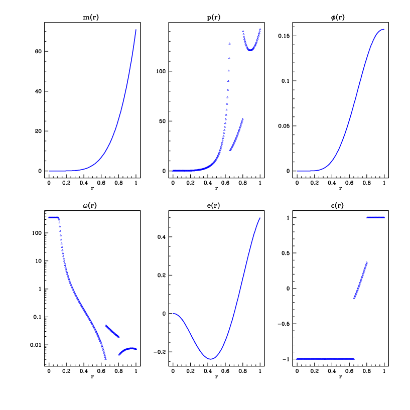
The resulting , , and are equal to the just calculated unsubscripted ones. In figure 3, an impression is given of how these simple prescriptions affect the evolution of a discrete shell universe.
Three more remarks are in order. Firstly, the scheme we outlined is not at variance with the second law of thermodynamics, since entropy clearly increases at collision time. Even in the theoretical and ”ideal” situation that no collisions occur anymore and the universe is cyclic212121As indicated earlier, we do not advocate this scenario, be it only because in a contraction phase the universe will rebound well before ”the point” is reached and at rebound time entropy will always increase., the dynamics of the universe, which is basically radial 2-body motion save for the effect of the cosmological constant, is not at variance with the second law, for the same reason as it is not an issue in cyclic 2-body motion.
Secondly, it is also clear that this scheme has important limits: there is no reason to assume that spherical symmetry is even indicated in the collapse phase. Be it for that reason only, the model in figure 3 is largely a toy model, illustrating some general principles, and should not be taken too seriously, certainly at later times, when the shells come close together and some chaos sets in. Surely other physics should be put in beyond the collisionless rather naive dynamical model that is presented here. Colliding shells would almost certainly break the spherical symmetry.
This touches upon a more general third remark. Cosmological models assume isotropy. There is a well-known rationale for this, and geometrical elegance and simplicity are important properties of the current cosmological models. If one breaks this perfect symmetry, then there is no particular reason to hold on to any other symmetry, such as the spherical one. Spherical symmetry is the first generalisation away from isotropy, and as such it has its merits, but one should not take the spherical non-equilibrium modeling too far.
5.2 The early history
A scenario for the early universe is of course completely speculative. In our paradigm, the universe may have originated as a black hole, in a ”mother universe” of which we will never be able to say anything, except for the fact that, perhaps, still now, material from that universe could enter our universe. In that early phase, at times very much longer ago than the currently accepted age of the universe, the universe must have been extremely hot, and filled with matter decomposed down to elementary particles and radiation. It would be a state similar to what is now our current view of the early universe, at a time when radiation decoupled. The big difference is that this state of complete chaos and mixing came about naturally. Matter and radiation of course did interact continuously, and the universe was initially too hot for any bound structure to develop. Hence entropy was maximized and the universe was in a homogeneous state in which particles whiz around, only, but irrevocably, confined by the horizon. The radiation field was, and remained, completely isotropic. This radiation was to become now the cosmic microwave background radiation (CMB). Note that in this scenario the CMB is in zeroth order isotropic by design, as must be any other field of weakly interacting particles.
Over (very long) time, the universe kept accreting matter, including probably vast amounts of elementary particles, and possibly also black holes. Once the latter were part of our universe, they may have become effective sinks of kinetic energy and matter. They did therefore their part in sweeping the chaos clean, and thus could have been a source of rarefaction. Pressure thus gradually decreased.
The larger the mass of the universe, the larger the event horizon. Matter, even bound structures, would eventually be able to enter the universe without being torn apart to elementary particles by the tidal forces at the event horizon, even without ’feeling’ the transition altogether . This could conceivably also have been a source of injection of bound structures.
Once our universe was sufficiently rarefied, filled with black holes of various sizes surrounded by matter, it entered the state in which we can start talking about structures, and hence comoving matter. At that stage our universe could be modeled with the scheme outlined in section 5.1.
5.3 The initial conditions of the present expansion phase
Of course, we may not bother about the earlier phases of our universe, and be content with the specification of continuous initial conditions. This option is also indicated if one takes the view, as seems to be strongly born out by the observations, that the constituent (dark) matter of the universe is unseen, and that a visible structure is but the top of an iceberg. In that case, the dark matter could very well be smoothly distributed, or at least much more smoothly than the visible matter. The CMB now can, of course, contain signatures of a previous phase (see e.g. Gurzadyan & Penrose [9], though we do not invoke or need Conformal Cyclic Cosmology).
Equation (2.23) can now be seen as a relation determining if or and the initial conditions (2.27) and at some are given.
In terms of the effective gravitating mass, we get the trivial recast of (2.23):
| (5.12) |
showing dat increases with increasing gravitating mass and decreasing . If at a finite , the initial conditions cause a universe. Note that in that case will be smaller than the Schwarzschild radius unless there, since here is the solution of
| (5.13) |
to be compared with which is the solution of (4.10). In general, we thus obtain a universe embedded in an inner Schwarzschild metric.
Alternatively, the expression of in terms of the mass function leads to a first order differential equation:
| (5.14) |
which can be solved for the energy , given e.g. the boundary condition . The integration can be carried out for under the constraint .
5.4 On the energy function and the effective gravitating mass
Here is the place to speculate on the behaviour of . We have seen in section 3.3 that , while from section 4.2.1 we have . This last condition is hard to change once established, unless one would invoke massive collisions of dynamically important (not necessarily comoving) shells, on scales of the size of the universe. As before, we forego for simplicity the likely breakdown of the spherical symmetry that this would entail. This reshuffling of shells and their kinetic energies would, according to equation (5.14), cause another , and probably also another and (even assuming that the total mass remains the same), much like the (simplified) scheme we outlined in section 5.1. It seems unlikely that the new would differ importantly from the old one, though, because this would lead to massive instabilities that probably would have been dealt with in the chaotic phases of the history of the universe.
The above considerations point to the possibility that the mass of a black hole can change with time, not only because mass is falling in, but also because what the outside world is measuring is effective gravitating mass, which depends on the kinetic state of the shells inside. We will return to this process from another point of view in section 7.3, where we will argue that there is evidence that it actually occurs.
In this paper we will adhere to the working hypothesis that the energy is rather close to 0, as seems to be indicated by the observations. Our definition of a universe then imposes that rises rather sharply to at the edge . Note that, according to the analysis in section A.3, this does not exclude universes that are largely homogeneous.
6 A classification of the universes
6.1 Preamble: the synchronous homogeneously filled universes
6.1.1 General formulas
In the case that and are constant functions throughout (note that we can drop the subscript in this section), we can lift all time limitations on the model since the initial condition will remain valid. Note that also and (representation (a)) are constant in that case, which means that we can also omit the explicit dependence of on as indicated in (3.3), and we obtain
| (6.1) |
which is separable in and . All relations that are specific for the central regions, as presented in section 3.3, hold now for all shells at all times.
The metric can be written as
| (6.2) |
with
| (6.3) |
which is obtained from (2.1) by changing the radial coordinate from to
| (6.4) |
using (3.5), (3.18), (3.22) and (3.24). We recognise the familiar Robertson-Walker metric, of course. We can identify
| (6.5) |
In the case we recall the well-known
| (6.6) |
where the radial coordinate was introduced which is inspired by the spherical embedding model. This implies
| (6.7) |
while the metric coefficients in the original metric (6.2) read
| (6.8) |
From the first of these equations also follows
| (6.9) |
in line with definition (4.2) of the radius of a universe.
The case follows immediately from the same formulae by substituting the trigonometric functions with hyperbolic functions, and the case by the limit in first order in . Hence, inside these universes, these synchronous spherical models are identical, locally, to the models used in standard cosmologies.
The effective mass function reads, with equation (3.21):
| (6.10) |
As for the ’s defined in (3.54), we recover, with the formulae in 3.3, the well known
| (6.11) |
The cumulative mass function can be calculated explicitly with (2.12). We obtain
| (6.12) |
These expressions, taken in , yield the total mass of the closed model, and approximations for the total mass of models with that are synchronous over most of the range and that have close to a steeply rising so as to have . We obtain
| (6.16) |
in units of according to (2.14).
6.1.2 The concordance model
In the current standard model, one finds that , and . With an age and a Hubble parameter of 0.74 (in our units), this implies, with equations (3.54), (3.55) and the formulas in appendix A.3, that , , and Gpc. The start phase can be interpreted as the end of an inflationary epoch. The shell label is, of course, undetermined.
6.1.3 The closed universes
We now turn to the synchronous universes that conform to our formal definition of a universe as embedded in an inaccessible outer space (section 4), which in this case implies , together with the relation (4.12) which states that . This expression provides an additional relation between the parameters.
The isometric representation is a hemisphere () with radius . Note that this representation is the same as for the standard closed cosmological model, except at the boundary . As already remarked upon in section 3.4.3, in this paper the hemisphere is not continued for to a full sphere as in the standard model: this universe has a center, and for we are revisiting the shell . It bulges out over the ’black disk’ with Euclidean surface area , yielding a hemisphere with the double surface area . Yet another way to appreciate the correctness of the picture without a ’lower hemisphere’ is to keep in mind that at the junction of the universe with the (Euclidean) outer space is continuous but not differentiable. However, one must envisage this universe as the limit of the dust ball discussed in section 4.1, which has a junction with the outer world that is continuous and differentiable. A small (local) disturbance could then ’pinch off’ the dust ball from the rest of space, thereby creating a universe. In that case, it is quite obvious that one doesn’t get a lower hemisphere ’for free’. In section 8.2 we will come back to the special status of the shell .
It follows from equations (3.18), (3.21) and (4.12) that
| (6.18) |
| (6.19) |
These relations imply that out of the three parameters , and (the parameter is an unimportant scaling factor of the dimensionless shell label) only one can be freely chosen. The most obvious choice is , as it is related to the Schwarzschild radius of the universe, but also would be a good choice, as it has the unit of mass density (which is one of our 3 primary units) and it is instrumental in fixing the amount of matter via (3.20):
| (6.20) |
Finally, with (3.22),
| (6.21) |
The smaller , and hence, the larger the mass, the larger the expansion time. Note also that the above relations imply that as should.
An interesting property of these models is that, contrary to the classical cosmological models, the magnitude of the mass density has no bearing on , since anyway. It follows from (6.19) that the density is merely inversely proportional to the square of the size of the model.
The total effective gravitating mass is poorly constrained by the Hubble parameter. The larger , and thus the smaller with (6.21), the closer the limit (3.49) is reached. For example, if we take and , we find , , , , and close to the critical density, since the rebound is very far in the future. This is to be compared with the case , where we find , , , , and . Note that these two very different values for yield similar ’s. Hence, there is, with as the only constraint at least, no useful upper limit on .
If we combine the expression for the radius of the synchronous universe (6.3) and the expression for the Hubble parameter (3.46), valid for large , we obtain
| (6.22) |
Hence, the larger , the smaller the fraction of the universe that will be visible for a given look back time, since the latter implies a fixed light travel distance. The horizon, measured relative to the size of the universe, therefore scales as . This result remains valid qualitatively for the more general universes we will discuss next.
6.2 The functions , and
In the general case that or are not constant functions of , the expression for is not separable anymore into a factor that depends only on and a factor that depends only on . This complicates the mathematics considerably. Also the relations (6.18), (6.19) and (6.21) do not hold anymore: the 3 parameters , and now form a 3-dimensional parameter space. In the sequel, we will adopt as our basic parameters , and , which is an equivalent choice due to (3.25). But there is much more additional freedom: in order to make the metric fully explicit, we need also to specify the free functions that appear in the radial metric coefficient .
Taking account of the boundary conditions at (subsection 4.2.1) and in the center (subsection 3.3), we now have to choose functional forms for , and .
We adopt
| (6.23) |
with . We will find it useful to also include the possibility to require that
| (6.24) |
and additionally to include the possibility that
| (6.25) |
Note that the synchronous is included if these additional conditions are absent and . The coefficients are determined in number and value by the optional requirements and the condition that is sufficiently smooth at . There are therefore 4 to 6 parameters: , , , the order of the smoothness of at , and possibly and .
As for , we also have to take account of the condition (2.15). We adopt
| (6.26) |
with . Again, the synchronous is included if . There are therefore 5 parameters: , , , and the order of the smoothness at .
Finally
| (6.27) |
with . The factor appears because . The synchronous has or . There are 6 parameters: , , , , and the order of the smoothness at .
Inside
| (6.28) |
the model is synchronous. When , the model is fully synchronous.
Though the above parameterisations seem rather necessary in order to include non-trivial functions , and , they imply already a rather daunting number of models that could be explored. In the sequel, we will assume , which is no restriction. For the asynchronous models, we will take and , since it seems reasonable to assume synchronicity in (the vicinity of) the center. Neither will we vary the order of smoothness of the junctions at shell . We also assume . This leaves us, apart from , and , with , , ( only relevant if ) and or .
As to the parameters , and , there is considerable freedom. Figure 4 shows a typical parameter space. There is essentially little constraint on on the high side, and the parameters and have there ’home base’ around the isotropic values.

6.3 The behaviour of the metric coefficient at the boundary
We define
| (6.29) |
and write, for , and thus
| (6.30) |
with ,
| (6.31) |
with , and
| (6.32) |
with
| (6.33) |
The above expressions make at the boundary explicit, and we obtain, after some calculations,
| (6.34) |
with
| (6.35) |
Note that in the vicinity of by our definition of a universe, that all 3 coefficients behave well at the boundary and that the three exponents , and are independent of time.
As a consequence
| (6.36) |
with
| (6.37) |
It follows that the volume element (2.11) of the metric, which equals upon integration over the angles, is integrable if
| (6.38) |
with the proviso that every statement about or inclusion of here and in the sequel is only relevant if . This shows that also volume is a relative notion, since the stretch in the radial coordinate can become arbitrarily large. In the limit, the space geometry at the boundary therefore approaches a cylindrical symmetry (see also subsection 7.1).
The inequalities in the no-collision condition (2.17) and the conditions (6.38) imply that either
| (6.39) |
if the term in in (6.34) ensures that , or
| (6.40) |
if either the term in or ensure that .
We note, for instance, that for the standard synchronous case and behave linearly at , and thus .
In fact, we can transform the radial coordinate into any other increasing function of it (see section 2.1). Since the function for while for , we could, locally, adopt as the new shell label. In that case . Hence parameter space could be reduced to .
Similarly, is a strictly increasing function in the vicinity of (recall that is the largest shell label on which comoving matter resides). Therefore we could, alternatively, adopt as the new shell label locally, and thus . Hence parameter space could be reduced to or .
We denote
| (6.41) |
From the conditions (6.39) and (6.40) we deduce
| (6.42) |
We retain the symbol , since in section we will assume different conditions from (6.39) and (6.40).
The asymptotic behaviour of equals
| (6.43) |
with
| (6.44) |
The above expressions are independent of the conditions (6.39) or (6.40). The parameter is thus a measure of the steepness of the singularity of at the boundary. The smaller , the more ’extra space’ there is in the radial direction as compared to the Euclidean case. We also note that the upper limit for , being , is only attained in case .
For the mass density, we find, using (2.6), for :
| (6.46) |
We briefly examine a few consequences in the case that for all , thus , under the conditions (6.39) or (6.40). If , then . If , then . If, however, the phase function is a constant in the vicinity of , then the first inequality disappears, , hence .
6.4 Alternative characterisation of a universe
The fact that for , for all , points towards yet another choice of shell marker. In the radial direction
| (6.47) |
showing that a change of radial shell marker proportional to will transform the metric locally at the boundary to a Lorentz metric. We will need such a transformation in section 8.2.
We could thus adopt a new variable with this behaviour at the boundary as an alternative shell marker. A possible choice would be
| (6.48) |
with given by (2.19) and the hypergeometric function. The transformation preserves order, and . Moreover we find
| (6.49) |
It reduces to (6.7) in the synchronous case () for .
With the transformation (6.48) we find that at the boundary
| (6.50) | |||||
This points to an alternative definition of a universe: its metric is such that the radial coefficient of the metric is regular up to the shell beyond which there is no mass, and for that shell , for all . Note that, because of the existence of the above transformation, the boundary is part of the manifold.
Though little would change in the paper (since is an arbitrary shell marker anyway), we do not make this choice here, and we leave the radial marker quite generally defined. However, it sheds another light on the condition if it occurs at some , such as happened in the early phases of the universe (see also section 8.2). Such a shell divides the universe into an inner and an outer universe, for as long as occurs.

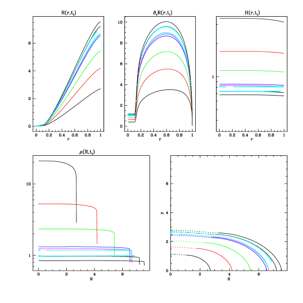
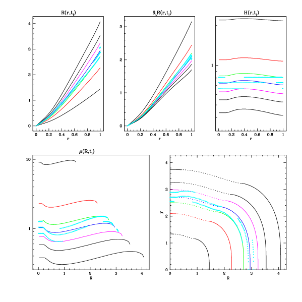
7 Between a dust ball and a universe
7.1 An example
We now discuss one particular class of models for which at some time , while is not singular nor zero, which is called a neck. Therefore the condition is not visible in the metric (the radial term is non-zero and is a ’de l’Hôpital’ type limit ). Out of this particular class we now consider the models for which , , and , which are of a class we excluded in the previous section.
Using (6.3) and (A.7) one finds that the metric approaches, for , the form
with here shorthand for , for clarity. Returning to the inner Schwarzschild- solution (4.14), we find that the time transformation
| (7.2) |
happens to be the same as (3.1), and we obtain
| (7.3) |
with again , which is identical to (7.1) upon relabeling the radial coordinate . Note also that the cylindrical geometry is quite obvious here, since both (4.14) and (7.3) show that the angular components of the metric are independent of the radial coordinate .
7.2 Mass ejection from a black hole
Next to impossible as a neck (for which is not singular and not zero) may be in the spherical case globally, the condition and finite may very well occur on a local scale with the spherical symmetry broken. From the asymptotic expression of in (6.36) it follows that
| (7.4) |
When both and are zero, i.e. when shells collide at the boundary , the boundary could be crossed, and if this happens at maximum expansion,222222In the other cases the crossing material would enter the space between the universe and the Schwarzschild radius, where only inward motion is possible and this material would therefore instantaneously enter the universe again with a locally Lorentzian outward velocity. matter and radiation could leave the black hole. Clearly, it remains a tough act to climb the gravitational wall in order to reach an outside observer, but since the radial coefficient is locally and temporarily regular, this is perfectly possible. We are then in the condition of a dust ball (section 4.1), without Schwarzschild- radius. This condition may also be relevant for ’small’ and rotating black holes (recall that the Kerr solution at the poles is locally very similar to the Schwarzschild solution), because, according to this mechanism, matter and radiation could escape from the poles of a rotating black hole, thereby causing periodic bipolar outbursts.
7.3 On the anomalous redshifts
We can also make a connection with the so-called ”anomalous redshifts”. This phenomenon, which has been around for about 50 years now, comes down to the assertion that high redshift quasars seem physically associated with low redshift, relatively nearby and active galaxies. This interpretation has been lifelong advocated by H. Arp, though the vast majority of the astronomical community interprets these redshifts as cosmological, and puts the phenomena aside as merely chance alignments and projection effects. It does not help, of course, that there is no obvious physical explanation for Arp’s interpretation. An accessible and short report on the phenomenon by Arp himself can be found in Pecker & Narlikar ([10]).
Since we argued in the previous subsection that, under specific conditions, material can leave a rotating black hole at the poles, we can see that the ”quasars” can be explained as being such material. That material has to climb a large potential well, though, hence the redshifts observed are largely gravitational. A particularly nice example is the Seyfert NGC 3516 @ , which has 6 X-ray sources @ aligned along the minor axis that are bipolarly distributed. Moreover, sources with higher redshifts are closer to the galaxy than those with the lower redshifts. This we can (qualitatively) explain by the overall mechanism of the ejection. At ejection, the radial coefficient of the metric, which used to be , is finite but of variable magnitude depending on the details of the shell collision. The higher , the more space will have to be crossed in the radial direction, the higher the reddening will be and the more momentum will be lost. Hence the ejecta with the highest momentum at exit, that therefore get the farthest out from the galaxy, will be the lesser redshifted. In other words, the redshift is inversely proportional to the ease with which the material could escape. Of course, this assumes that the initial momentum prior to ejection is for all ejecta similar, which need not be the case.
The case NGC 3516 also shows that the ejection can be recurrent, as demonstrated in the ‘ideal’ case of section 7.2. Therefore NGC 3516 is actually also in this respect corroborating evidence for the physics proposed in this paper.
In this context, the issue of quantized redshifts is never far away. It is conceivable that there is some relation, but in this paper we will not pursue this issue.
8 Orbits
8.1 The equations of the motion
Due to the spherical symmetry, the motion is planar and we choose any meridional plane . Hence we can adopt the metric
| (8.1) |
leading to the following set of equations for the geodesics:
where is the specific relativistic angular momentum (a constant), and differentiation with respect to arc length is denoted by a dot.
Instead of , which is the shell label change rate with proper time along the orbit, we introduce the local Lorentzian radial velocity component
| (8.2) |
This leaves us with the following system of 5 coupled first order differential equations:
| (8.3) |
where we also introduced . We note that, interestingly, the has disappeared.
The initial conditions are given by the coordinates and the Lorentzian components of the velocity
| (8.4) |
Since we have an additional constant of the motion following from the metric (8.1):
| (8.5) |
where for a massive particle and for light, we have also
| (8.6) |
which completes the necessary initial conditions. The quantity is therefore the relativistic energy relative to the rest mass energy as measured by a comoving observer :
| (8.7) |
In the actual integrations we make no use of (8.5), since efficiency considerations are not critical, and (8.5) can rather be used to check the accuracy of the integrations. Also, we replace the derivatives on the left hand sides of (8.3) and (8.17) with , which means that the right hand sides are divided by . This has the advantage that the independent variable of the orbits is the cosmic time, on which all observers agree. We retain the information on the arc length by replacing by
| (8.8) |
8.2 The orbits at the boundary
8.2.1 The equations
The function is singular. In order to carry the integration over that limit in a stable way, we set
| (8.9) |
with
| (8.10) |
and defined in (6.41). Inversion leads to
| (8.11) |
We refer for this choice to section 6.4, where it was shown that such a change in shell label transforms the singular metric at the boundary into a Lorentz metric. We denote
| (8.12) |
As a consequence of the introduction of this new shell label , the disk is now covered by 2 sheets, one for , or , and one for , or .
In order to verify that the coordinate transformation (8.11) is consistent with the radial velocity , we write in terms of and :
| (8.13) |
with
| (8.14) |
When , remains finite if and only if, taking into account the asymptotic behavior of in (6.43), definition (8.10) holds. Hence we find
| (8.15) |
With the expressions (8.13) and (8.14) we see that is a step function at . This follow also from (8.2), since changes sign at ( at ). The velocity is thus the Lorentzian radial velocity on sheet and the negative of it on sheet . We would thus need to stop and restart the integration upon arrival at that shell. We can avoid this by defining
| (8.16) |
where we used (8.13). This makes the true local Lorentzian radial velocity.
The equations involving and in (8.3) now read
| (8.17) |
These equations behave well at . The appearance of in (8.17) is a consequence of the shift from to the Lorentzian , since we need to take account of the sign of .
In the case that throughout, we can keep the same formalism, except that we now define :
| (8.18) |
Clearly, there is only one sheet.
Of course, we can arrive at the same conclusions with respect to the behaviour of in the vicinity of the boundary solely from an analysis of the geodesics (8.1). The first equation can be rewritten as
| (8.19) |
It reduces for to
| (8.20) |
taking into account (6.43) and (6.45). The fourth term tends to zero, and we retain
| (8.21) |
There is an exact solution for such an equation, in the assumption that
| (8.22) |
is slowly varying (thus assuming it to be constant). In that case the equation does not explicitly depend on , and a substitution yields a first order linear differential equation in . We find the following solution, including the condition :
| (8.23) |
with an arbitrary constant.232323In the general solution, the other arbitrary constant is a shift of the origin, since (8.21) does not depend explicitly on (assuming to be a constant).
8.2.2 The physical nature of the boundary
The definition (8.16) has a very physical rationale: a traveler (not comoving) who arrives at the boundary will not experience a jolt of any kind, but will simply continue his/her journey ’outwards’, though he/she will move ’inwards’ because he/she revisits shells with decreasing label . This must, as it is a consequence of the analysis in section 4.2.2: if a particle would travel ’beyond’ , it would enter the space-time between and the Schwarzschild radius where outward travel is impossible. The strange situation thus occurs that our outward traveler will at the boundary have to change , which is only of relevance with respect to the shell labels in the universe, not locally. Put differently, an observer who sends a projectile outwards (e.g. on an inertial track), will get it back, but with opposite .
All orbits that reach the boundary will thus reflect from the boundary in the picture: tangential velocity is conserved, shell label change rate flips sign. The boundary is therefore a gravitational mirror. If close enough to the boundary in order to allow for short enough light travel times, one could see 2 images of the same object, or actually see oneself in the mirror (but at an earlier epoch).242424This is of course not different from a mirror as we know it in daily life, but there time differences are of the order of s. In a cosmological setting these images would correspond to different ages, and different aspect angles, so these would be hard to identify. The only (theoretical) way an observer could ascertain his/her position as being on the boundary, and at the same time detect the direction towards the center, is by identifying 2 lines of sight, in opposite directions, that contain the same objects, as one would do with an ordinary mirror. The radial direction is the only one on which one would see the same objects, with the same aspect angle and the same age (but see next paragraph). One way to distinguish which direction is the outward one is to observe additional objects, which are to be found in the outward direction since these are falling in from the mother universe. Barring these, one could state that, in some sense, ’inward’ and ’outward’ do not exist there.
We now investigate what happens with the spin of an object when it arrives at the boundary. Since spin changes sign when reflected in a mirror, we can expect that the spin, as defined with reference to the universe, will change sign after touching the boundary. To see intuitively how this works, we first consider a comoving observer who sees a spinning traveler. Both are close to the boundary. Both will see the local universe direct and mirrored: the observer thus sees the traveler in a direct image and in a mirrored image (just like an ordinary mirror), and these images will have opposite spin. When the traveler approaches the boundary, the observer will see both images of the traveler coming closer together. When the traveler is sufficiently close to the boundary, the light paths towards the observer will eventually coincide, and the observer cannot tell which image of the traveler is direct, and which image is reflected. After that, both images will again part. None of the images change spin, they ’only’ exchange the adjectives ’direct’ and ’reflected’. Of course, the traveler didn’t physically change spin, as defined with reference to his/her own local reference frame. In other words: suppose that the traveler leaves the observer on a journey, and both have (thus) had the occasion to physically ascertain their relative spins. When, after recoiling at the boundary, the traveler returns to the observer, both will find the other with a spin opposite to the spin at departure. Stronger still: when you send off a right hand in the radial outward direction, you will get a left hand back, since it literally and physically flew into its mirrored world.
What is the point of view of the traveler with respect to the universe? As he/she approaches the boundary, the hemisphere of the local universe centered around the anti-center will start to look like the hemisphere of the local universe centered around the center , up to the moment that they are equal upon arrival at the boundary (suppose no infalling material or radiation from outside the universe). The 2 directions towards the ’center’ are then on 2 diametrically opposite points. Suppose now that the observer’s spin is tangential, i.e. perpendicular to the direction of the center . The plane perpendicular to his/her spin we call the horizontal plane, and we call the zenith the direction of his/her spin vector. How could the traveler determine his/her spin with respect to the universe? He/she could look at 2 standard stars and on the horizon with an angular separation of, say, a few degrees, and observe which of the stars passes first his/her line-of-sight. Let be left from , and right. Thus passes before (northern pole rotation). This is a clear procedure if far enough from the boundary, but when approaching the boundary, the region around the anticenter increasingly starts to look like the region around the center , as already indicated. At the boundary, the mirror image of is now left from the mirror image of in the direction , and the mirror image of is now to right. Hence passes before , causing the determination of the opposite spin. The same effect is also clear when looking perpendicular to where you see the mirroring right in the field of view. On the boundary, there is no way to tell ’direct’ from ’mirrored’. Right after touching, the direct image becomes the mirror image and vice versa. After some time after touching, the mirror images disappear, and the determination of the spin will be permanently towards the nadir. Again, the traveler didn’t change spin, the image of the universe did.
Clearly, physically, there is nothing special going on. Our ’outbound’ traveler is continuing traveling in his/her view in an outward direction (not necessarily on a radial orbit of course): his/her orbit has no turning point, except in a coordinate system that has a singular radial metric coefficient, such as but unlike the local Lorentzian system. The effect is apparent in the sense that it is the universe that presents itself ’upside down’. In order to make this clear, we recall that in the standard cosmological picture of a closed universe as the surface of a complete sphere, the traveler simply would have passed from the ’upper hemisphere’ to the ’lower hemisphere’, and would continue exploring new horizons. Not so here, as explained in section 3.4.3. Our outbound traveler flies towards and into the mirror image of his/her universe.
We now decompose the spin vector into its radial component and tangential component. The radial component will not flip when touching the boundary, the tangential will. Suppose that the observer emits a photon radially outward. Because of helicity, it has a spin with only a radial component. He/she will get that photon back, but with the opposite helicity: parity is not conserved. The boundary could therefore be a model for spinor-like behaviour. We recall that at the boundary, space is as Lorentzian as anywhere else, since the singularity in the coordinate system can be transformed away (section 6.4). Hence the analogy of the sphere is locally valid.
This brings us to yet another characterization of the boundary. Instead of passing from the upper hemisphere to the lower hemisphere as in conventional cosmology, the outward traveler passes from the upper side of the (only) hemisphere, to the underside of the (same) hemisphere. Hence, when the traveler happens to return to the shells he/she has already visited on his/her outward journey, he/she will find everything left handed that used to be right handed, and vice versa! In the synchronous case 6.1, this translates into ’standing on’ the hemisphere for and ’hanging down from’ the same hemisphere for . Spin and helicity are proportional to .
Finally, the boundary is a special place because there material objects and photons can appear ’out of nothing’, i.e. they are falling into the universe. As already noted in the discussion connected with (4.20), they can have any radial velocity in the local Lorentzian frame, including thus positive ones.
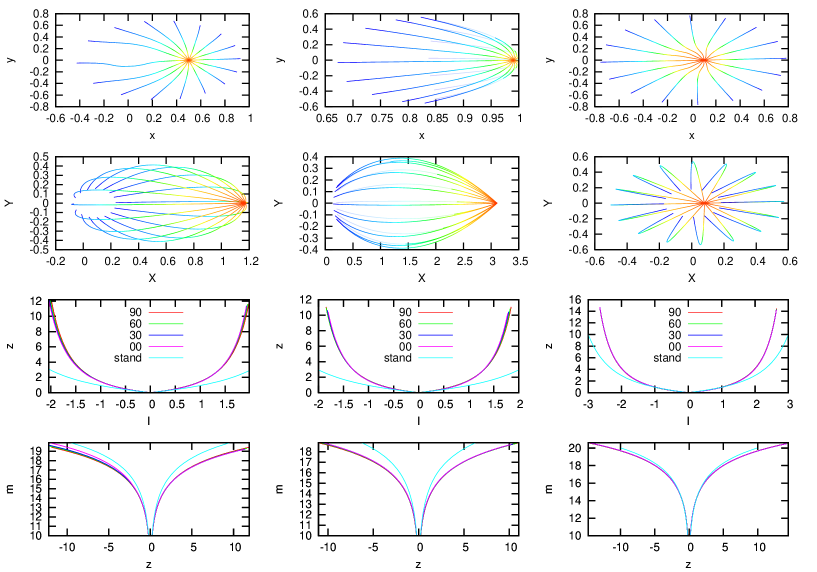
Third row: the Hubble law for different directions (indicated in degrees) and compared with the standard model. Negative correspond to the indicated angle . The Hubble law is very similar in all directions, which is by design, since and do not differ by more that 10%. From the middle column it is clear a recoil from the boundary has no effect on , showing again that the boundary is not a locus of singularity.
Bottom row: the magnitude-redshift relation for objects with an absolute magnitude of . Negative again correspond to the angle . The colours have the same meaning as on the third row.

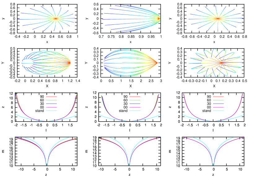
9 Light
9.1 Redshift
The redshift is calculated by considering 2 photons separated by 1 light period , on paths and , as seen by co-moving observers. Since equals the wavelength (), is the wavelength change on the path over a , and hence the change in the redshift over that . From (2.1) we have and , , so we can use the theorem in appendix C, more in particular (C.10), which states that is a constant along the orbit, and thus
| (9.1) |
The second equality expresses the assumption that the photon is emitted at in the rest frame.
Since we have available from the integration, we can calculate redshifts as follows. Suppose we integrate forward in time between 2 cosmic times , and consider a photon with wavelengths and . Then
| (9.2) |
When we integrate backward in time between 2 cosmic times , we obtain
| (9.3) |
In the latter case, is the time at emission , and we recover of course the well-known
| (9.4) |
In order to derive the Hubble law, we use (8.5) and (C.4), the latter of which reads
| (9.5) |
We obtain the following differential equation for the redshift along a light path:
| (9.6) |
For a light ray making an angle with the outward pointing radial direction, we can set
| (9.7) |
The Hubble law expresses redshift as a function of the geometrical distance from the emitter to the observer at some time , at the state the universe is in at . It is therefore only meaningful if the universe did not change appreciably during the travel time of the photons. If we insist on without restrictions on the size of , though there is no photon that could ever have traveled that , this distance satisfies
| (9.8) |
which can be added to the set (8.3). Locally, we have
| (9.9) |
Since in this paper , the replacement of the derivative with respect to with a derivative with respect to t would result in multiplying the left hand side with , yielding the familiar velocity .
Equation (9.9) gives us occasion to define the radial Hubble parameter
| (9.10) |
and thus
| (9.11) |
In the limit and for the current epoch , we obtain for (9.9)
| (9.12) |
We see that in principle we could recover the Hubble parameter in its standard definition by observing the velocity-distance relation in directions perpendicular to the center of the universe. The above equation provides also a means to detect the direction of the center of the universe in a perfectly spherical world.
9.2 On the relation between and
In the general case, is quite independent of the tangential Hubble parameter . In the synchronous case everywhere, though.
It is not hard to produce models for expanding universes, which have (of course), while in some parts! Since we can exclude these occurrences, such as others whereby and differ by more than, say , this constraint is an important one in order to select regions in a model that suit the observational constraints. Note however that in the center and therefore this constraint is of no significance in the central regions of any model we consider in this paper.
It turns out that
| (9.13) |
The sign of is thus the same as the sign of .
We can make this qualitative statement somewhat more quantitative when we express as a function of and as we know from (3.3). We find
| (9.14) |
The appearance of makes it clear that the phase function will be instrumental if it is desired to keep close enough to .
9.3 The observed surface brightness and flux
Because isotropy is lost in the spherical case, an expanding light cone will not generate a constant flux on its surface. Therefore we have to analyze the transformation of surface brightnesses and fluxes in a more fundamental manner than what is sufficient in the isotropic case.
Consider 2 photons that are emitted in directions that differ infinitesimally by . They will separate from each other along the light path by an infinitesimal distance , perpendicular to the path. In the Euclidean case we have
| (9.15) |
with the geometrical distance, and this expression is valid independent of direction and place of emission. The above expression is the basis of a flux calculation. It is also known as the angular distance, often denoted by . We will need to define at observer and emitter, and respectively (appendix D). In our case, the above expression is only an approximation for small , because here depends on the light ray, and must be calculated via an integration. Obviously, this complicates flux calculations considerably. To that end we derive in appendix D two additional differential equations (D.13) and (D.14) that add to the equations for the light ray.
In appendix E.1 we calculate the surface brightness along the light ray (E.7), defined as the power of the light ray at a certain wavelength , within a wavelength range and an elementary solid angle , and incident on an elementary surface . As is well known, and contrary to the Euclidean case, it is not a constant anymore.
9.4 The light ray for small orbit parameter
9.4.1 The light ray
We find in the vicinity of or , with , in first order in
| (9.16) |
or
| (9.17) |
In these expressions, and . When , we have to go to second order. We find
| (9.18) |
or
| (9.19) |
again, with the obvious notations and . On the boundary, expression (9.16) remains valid, while for the shell label
| (9.20) |
The case and yields the only ’circular’ orbit, as remarked upon at the end of section 8.2.1.
For we find easily
| (9.21) |
For the light ray has .
Equally straightforward is the expansion
| (9.22) |
The radial velocity reads
| (9.23) |
with
| (9.24) |
and shorthand for (and similarly later on for ). The coefficient is never zero, except on the boundary when which is the case of the circular orbit .
As for the relative energy, we know from classical cosmology that, in order to dig out the deceleration parameter, we will need to go second order:
| (9.25) |
We find
| (9.26) | |||||
For the second order coefficient we introduce
| (9.27) |
together with
| (9.28) |
We note that and have the dimension of inverse length, while , , and are dimensionless. We also recognize in the familiar deceleration parameter of classical cosmology.
9.4.2 The photometry
We start with the the expression for . Despite the relative complexity of the relevant differential equations (D.13) and (D.14), we obtain to second order in , after quite some calculations
| (9.33) |
indicating that the second order term is identically zero. This absolute value is a consequence of . This expression is valid at any point along the light ray. However, the expressions (E.7) for the surface brightness and (E.14) for the apparent magnitude feature and .
The expression for is the easier one. We need to integrate the light ray backwards (thus backwards in time). Hence the observed redshift is, with (9.3) and (9.25)
| (9.34) |
After inversion and insertion in (9.33) we obtain
| (9.35) |
To calculate , we must integrate a light path from the emitter to the observer, hence the parameter at emission time and at the observer . The result needs to be expressed as a function of redshift according to (9.2). This means that the expression (9.25) has to be expanded at the emittor, who has :
| (9.36) |
For we can in (9.29) simply replace the subscript 0 on the right hand side with subscript o since that term is second order:
| (9.37) |
For we need to write the right hand side of (9.26) in terms of the observables with subscript o via a first order expansion. This proceeds by writing
| (9.38) |
which we transform with (9.17) and (9.22) in
| (9.39) | |||||
After some calculations we obtain for (9.37)
| (9.40) |
with
| (9.41) |
and
| (9.42) |
9.5 The synchronous universe
9.5.1 Light paths and the horizon
It is useful to relate the general analysis above to the well-known standard cases. The metric (6.6) can be rewritten in the 2D case as
| (9.46) |
We will first consider a radial light ray . The last 2 equations of (8.17) easily combine to the constants of the motion
| (9.47) |
while the first equation of (8.17) produces
| (9.48) |
which also follows, of course, directly from (9.46). We assumed a light ray that arrived at the observer at and cosmic time from being emitted at on an earlier time .
We can be more explicit regarding (9.48). We express it firstly as a function of the state , initially defined in (3.2) as the state of shell at , but here it can be taken as the state of the universe at . Clearly
| (9.49) |
Next we assume that is not larger than 1 period, or, with the notations of (A.5)
| (9.50) |
Passing to the new variable , we obtain, with the notations of appendix A,
As was already pointed out in sections 3.4.3 and 6.1.3, this is only formally the same analysis as in the standard Robertson-Walker models: here the center and the boundary are special places globally (not locally). The case corresponds to and the case corresponds to . Moreover, the circles with radii and are to be identified. A radial orbit is different from a general orbit, because the center is a special point. However, looking at these general orbits, they appear as ‘great circles’ in an embedding diagram (see section 3.4.3), just as the light rays in the figures 8, 9 and 10 suggest paths that are similar to great circles. Hence one could, for every great circle, define a radial angle similar to . We will need this extended definition of in chapter 13.
Finally we note that the expressions (9.5.1) can be used to calculate the horizon during a finite time lapse. We assume the start of time at . It thus suffices to substitute in the first equation:
| (9.52) |
This integral is evaluated in equation (A.78). As an example, we consider the case of a closed universe with . At maximum expansion and we obtain, with and (the cubic in (9.5.1) is reduced to linear) that . At that time, every object is visible twice: once in a direct image, and once in a reflected image. This is obvious for an observer at the center , but holds for every observer if we consider the angle .
9.5.2 Photometry
As for the redshift, we use (9.3) and (9.47) to get the familiar
| (9.53) |
with and the radii of the universe at the time of emission resp. the time of observation.
For the parameters introduced in the previous subsection, we find (omitting all subscripts o)
| (9.55) |
and
| (9.56) |
All this yields
| (9.57) |
and
| (9.58) |
In this case however, we can do better. From geometric considerations (the paradigm of the inflating balloon) we can see that
| (9.59) |
with the normalised radial shell label (2.19) of the observer if the emitter is placed at (which can always be arranged for). The rod is now placed perpendicular to the plane of the light ray (say a meridian) and hence a is a small arc length on a small circle subtended by a which is now actually a . The radius of the small circle is . Unfortunately, this nice trick works only if the embedding diagram is a circle (and thus the 2-D universe a sphere).
Turning to the surface brightness, we see from (E.7) that we need the product
| (9.60) |
in first order in . Apparently, has disappeared.
Hence
| (9.61) |
(actually also ), and we obtain, using (9.53), for the transformation of the surface brightness (E.7) the well-known relation
| (9.62) |
Now we also see that (9.60) is the first order expansion in of .
As for the transformation of the fluxes (9.4.2), also that expression is considerably simplified. We recover the familiar
In this case, one can actually obtain an exact expression, for that is. It is called the expression of Mattig, and in order to derive it one uses the well-known parametric expression for cyc. For a much more complicated parametric expression for cyc can be derived, using as given in (9.48) as the parameter. However, it involves elliptic functions and the roots of the cubic (see app. A), and is therefore unlikely to lead to a closed expression.
One can easily prove that the (locally) synchronous models are the only ones for which in a finite region of space and therefore the only ones for which is direction independent.
9.6 Comparison with observations
The obvious observational effect of the spherical cosmological models we consider here is the directional dependence in the classical observational tests. The relation shows a quadrupole effect, and the relation has in addition a dipole term. Studies, such as the one by McClure & Dyer [11], that look for so-called anisotropies in the Hubble flow, focus on anisotropies that are caused by relatively nearby disturbances (such as the great attractor). It will be hard to separate these disturbances from the effects of a spherical cosmological model in the large, and this in the presence of important uncertainties in the interpretation of the raw observations.
We now work out the relevant quantities in the Hubble law as given by (9.12) and the magnitude-redshift relation as presented in (9.4.2) for the simplest possible non-trivial model for a locally flat universe: the one with given in appendix A.3.2. Since the shell label is arbitrary anyway, we can suffice with and thus
| (9.65) |
Note that this particular choice for endows it with the dimension of a length to the power 1/3. Since we have
| (9.66) |
A prime denotes derivative with respect to shell label , and we will in the sequel omit the explicit notation for the shell label dependence of . Since
| (9.67) |
we have directly an estimate for , about 9 Ga, and an alternative form for
| (9.68) |
Next we find
| (9.69) |
The 2 parameters and are sufficient to fit the Hubble law, including the quadrupole. and then yield . The deceleration parameter
| (9.70) |
as also follows from (3.37), and
| (9.71) |
Both and therefore are fixed if the Hubble law is known to sufficient accuracy. The other parameters in the relation are
| (9.72) |
featuring additionally the parameter , and finally the rather messy looking
| (9.73) | |||||
adding to the parameter list. Clearly there is enough freedom to fit and , even if the data are good enough to contain directional information. Finally, as already remarked upon in subsection 9.2, the phase function comes to the fore as instrumental in the fitting process.
10 Primordial black holes
One of the important discoveries in the field of dynamics of galaxies within the past 15 years is the strong evidence for super massive black holes in the center of galaxies. In addition, a reasonably well established correlation exists between the mass of the central black hole and the mass of the galaxy (including dark matter, see e.g. Baes et al. [12]). This points to a scenario in which at least some black holes were primordial, with the galaxies and the dark matter subsequently accreting around them.
We now investigate what happens in the vicinity of a black hole when the universe is in a collapse phase. We start with the standard equations of the motion around a Schwarzschild black hole, with the metric (4.3) and . There are 2 constants of the motion. On the one hand
| (10.1) |
with ’’ not te be taken literally, but standing for ’sufficiently far from the black hole where general relativistic effects are negligible’, the rest mass of a test particle and
| (10.2) |
with the mass of the black hole.
On the other hand
| (10.3) |
with the proper time on the geodesic. The expression (10.3) is identical (up to factor ) to the third equation of the cosmological geodesics (8.1). This is relevant, since on small scales the universe can be considered synchronous, and the black hole could therefore be taken as the center of the universe, and thus in the center of a spherically symmetric field. The metric yields
| (10.4) |
with
| (10.5) |
the effective potential. In this expression
| (10.6) |
We now analyze these effective potential curves (10.5), and refer to fig. 11.
The derivative of equals, apart from a factor ,
| (10.7) |
The effective potential has 2 extrema for at the radii :
| (10.8) |
with for the maximum at and for the minimum at . We find the following expressions for the maximum and the minimum :
| (10.9) |
A particle with negative radial velocity will fall into the black hole if one of the following three conditions is satisfied:
-
1.
. The parameter is therefore the smallest value for that allows non-plunging orbits.
-
2.
is smaller than the smallest radius of intersection of with .
-
3.
. The parameter is therefore the largest value of the energy for a given that allows non-plunging orbits if the radial velocity is negative.
It follows that
-
i
a particle that has negative radial velocity and finds itself closer to the black hole than the minimum of all will plunge into the black hole. This minimum occurs in the limit for and equals
-
ii
a particle that is farther away than the maximum of all will never be in condition (2). That radius is .
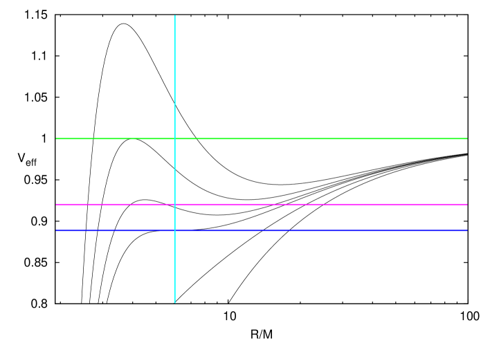
From (10.1) we see that in a collapsing synchronous universe will increase, since is a constant and therefore the magnitude of the velocity far from the black hole will increase. On the other hand, the angular momentum is a constant both in the Schwarzschild metric and in the cosmological metric. Hence the effective potential does not change during the collapse. It follows from the form of that material that was originally in a stable orbit around the black hole will find itself on an increasingly more radial orbit and, at some moment in time (during the part of the orbit with negative radial velocity) finally on a plunge orbit. The higher , the more rapidly the fall will be. Hence the black hole will start to accrete matter it would never have accreted in a static universe. Therefore, the stronger the collapse phase, the more massive the black holes in it would grow. In the limit, a black hole in the center of a synchronous universe would accrete all the matter in the universe! But as already mentioned before, this is not the scenario that is being advanced in this paper as a likely one,252525Note that no fundamental changes would have to be made in this paper in order to include a black hole at the center of the universe. Instead of we would simply have to assign a non-zero value to . though that scenario is in line with the concept of a universe inside a black hole. Instead, the collapse would probably halt much sooner, at various places and at various times,262626Recall that clusters of galaxies occur in spongelike structures. and the material that was lucky enough not to fall into the black hole, would simply be a galaxy in the newly started expansion phase of the universe.
In the sequel we will also need the inverse of (10.9) with , yielding the angular momentum that corresponds to an effective potential curve that has a given at its maximum. Somewhat surprisingly, that inversion can be written down explicitly:
| (10.10) |
As a bonus, essentially the same calculation yields the angular momentum that corresponds to an effective potential curve that has a given at its minimum, or, more physically phrased, the angular momentum that corresponds to the circular orbit with given :
| (10.11) |
This result can be linked with the elementary result for circular orbits in the Newtonian limit, here for large , which is
| (10.12) |
hence or . On the other hand, if we set , hence , we obtain from (10.11) that and therefore , as should, since . .
11 Dark matter
11.1 Introduction
The inclusion of dark matter must be part of any cosmology. The proof of its existence rests essentially on the dynamics of galaxies and clusters of galaxies, and is most obvious in an analysis of the rotation curves of spiral galaxies.
Neutrino’s are not considered to be viable candidates for dark matter in the standard cosmology, because, in order to be effective, their masses and/or their densities would need to be too high to allow for an open universe. In the model we consider here, the universe is closed by design, and this argument disappears. Moreover, in this paper we cannot invoke much a priori information about the latest compact phase of our universe, so from that side no useful constraint is to be expected. In this section we therefore investigate more closely the possibility that dark matter is constituted ’simply’ of neutrino’s. Clearly, this has been looked into earlier (see e.g. Paganini et al. [13] for the case of galaxies and Nieuwenhuizen [14] for the case of the galaxy cluster Abell 1689). We will discuss this now again, in the context of the universes we consider here.
In the same vein as we argued that in our paradigm the CMB is isotropic of necessity, we can probably say the same about the cosmic neutrino background (CNB), at least for those neutrino’s that have been around for multiple expansion and contraction phases.272727The CNB is not to be confused with the neutrino flux at higher energies, which is, just as radiation, highly anisotropic. For a speculative picture of the early stages that we refer to, see section 5.2. We will consider Fermi-Dirac or Maxwell-Boltzmann distributions. It must be stressed that our analyses are equally valid for any dark matter candidate, as long as it satisfies (approximately) a Maxwell-Boltzmann distribution, which is what nature tells us that it must (see section 11.4).
11.2 The field equations
We will assume that the mass distribution has selfconsistently settled down in a steady state around a mass concentration. We will continue to use the notations employed in chapter 10. For a mass of we find , and we define as in this unit:
| (11.1) |
In the general relativistic case, we assume the following metric:
| (11.2) |
The Einstein field equations determine and (see Landau & Lifshitz, [15]). The function is determined by the first field equation
| (11.3) |
In analogy with the Schwarzschild case, we denote
| (11.4) |
and find
| (11.5) |
We note that (11.5) is essentially identical to (2.6), and we therefore know that is the gravitating mass function (with unit length). Passing to dimensionless quantities:
| (11.6) |
with the dimensionless mass density expressed in and . If we denote by the radius inside which there is no mass, then if follows from section 10 that and .
The mass function clearly follows from the metric (11.2) and (11.4):
| (11.7) |
In the Newtonian case
| (11.8) |
and we recover of course the familiar
| (11.9) |
The function is connected by the second field equation
| (11.10) |
with the radial pressure . Again, we write the function as
| (11.11) |
The function plays the role of a general relativistic gravitational potential of the distributed matter around the black hole, and . We obtain
| (11.12) |
with the dimensionless radial pressure expressed in . We omitted the explicit dependence on of , en for clarity. Denoting
| (11.13) |
we can cast (11.12) into the form
| (11.14) |
or, returning to ,
| (11.15) |
Because of the signature of the metric, or with the equality only possible if .
In the Newtonian limit () and for large (compared to ), equation (11.14) reduces to
| (11.16) |
Turning on the dimensions again, we find for (11.16) the well-known
| (11.17) |
if
| (11.18) |
which is therefore the Newtonian binding potential.
Alternatively, in the same limit, (11.12) becomes
| (11.19) |
which is also a known Newtonian result, since classical potential theory learns
| (11.20) |
for a mass distribution with finite total mass and boundary , and thus
| (11.21) |
Passing to dimensionless quantities, we find
| (11.22) |
identical to (11.19). Hence, in the Newtonian limit,
| (11.23) |
We don’t need the last 2 field equations
that involve the tangential pressures in order to determine and , since these equations follow from the first 2 by virtue of the fact that the divergence of the tensor is zero (). This property of a covariant 4-vector field yields again 4 equations. It turns out that 3 of them are trivial ’s. The remaining one gives rise to the equation of hydrostatic equilibrium:
| (11.25) |
The limit recovers the well-known spherical Jeans equation of stellar dynamics.
Finally we note that if we didn’t have a distribution function to derive and from, or an equation of state connecting the mass density and the pressures, the above equations would not suffice to determine them. This is, of course, a well-known feature shared with the Newtonian case.
Given expressions for and , the functions and or or are determined by integrating the equations (11.6) and (11.12) or (11.14) or (11.15) from the inside out, starting from , with
| (11.26) |
and a free parameter
| (11.27) |
However, since is the solution of the naked black hole. The physical interpretation of this parameter is best grasped from , since that is the general relativistic generalization of the depth of the potential well caused by the black hole and the matter around it.
Leaving the solution for for later, we still need to determine the solution inside . The solution of the ‘homogeneous’ equation (11.12) with and is
| (11.28) |
The linear term in also affects the constant in . With we find
| (11.29) |
Clearly a causes clocks to run slower than the rate of the naked black hole, as a consequence of the additional matter around it.
We will now consider two regimes where the neutrino’s manifest themselves quite differently.
11.3 Neutrino’s in the vicinity of a quiescent black hole
In this section we follow up on the formation of primordial black holes (chapter 10), and investigate what could remain around such a black hole as a result of a collapse annex accretion process. We need not consider since between and all matter falls into the black hole anyway (as explained in chapter 10), in the additional assumption that matter in that zone has entered that zone from the outside and was not launched in it from the inside. Note that this (mildly) invalidates the assumption of steady state, since the black hole will grow, but we assume that this growth, after the formation process, is slow.
11.3.1 The orbital dynamics
When integrating over the dark matter distribution, we should only include those that are not on plunging orbits, since we can assume that all material on them has crashed into the black hole. Therefore we reconsider the analysis that let to the infall conditions in section 10, but now for the metric
| (11.30) |
with
| (11.31) |
We find
| (11.32) |
with
| (11.33) |
These expressions are the obvious generalizations of (10.4) and (10.5).
From fig. 11 we can surmise that, also in this case, the effective potential curves have 0, 1 or 2 extrema for finite . In the case of 2 extrema, occurring at , the smallest is a maximum. The extrema can be found rather explicitly using the second field equation (11.10), which we first recast, with the help of (11.4), in the form
| (11.34) |
This enables us to write the extrema of the effective potential (11.33)
| (11.35) |
as the solutions for of
| (11.36) |
somewhat remarkably in a rather closed form with no explicit differentiation involved. For the Schwarzschild case and , and we recover (10.7). Clearly we cannot make the solutions of (11.36) more explicit without knowledge of and , but we will assume that the conditions for infall will be qualitatively identical to the ones stated in section 10, on which the figure is based.
Since for physical reasons , the left hand side of expression (11.36) has the same sign as , and thus has maxima and minima in the same positions. That left hand side therefore is
-
i
positive if is smaller than the maximum of
-
ii
negative if is between the maximum and the minimum of
-
iii
positive if is larger than the minimum of
if these extrema are present (this depends on ). In the first case we are on a plunging orbit, in the second and third we may, depending on .
11.3.2 The dark matter response density
In order to obtain the response dark matter density, we first rewrite (10.3) as
| (11.37) |
with
| (11.38) |
the tangential component of the velocity, the time measured by a stationary observer at and
| (11.39) |
the relativistic energy, normalised to the rest energy, measured by the same observer of a moving object with proper time . In terms of the normalised quantities we introduced so far, we obtain for the tangential component of the linear momentum
| (11.40) |
which also defines the dimensionless .
All this prepares us for the use of (F.7), after passing to dimensionless quantities:
where a distribution function normalised so as to produce a mass when integrating over a volume in phase space.
As to the integration limits, the upper bound in follows from (F.3) and the fact that we consider only dark matter particles that are permanently trapped around the black hole, hence . We recall that the upper bound in can be understood by the requirement (11.32) of positive squared radial velocity
| (11.42) |
We note that this inequality, or alternatively (F.4), is consistent with the expression
| (11.43) |
with the dimensionless radial momentum, defined in analogy with . The upper bound in the integration of is therefore .
The lower bounds in (11.3.2) are not specified, because we have yet to exclude the plunging orbits, and this needs a more careful analysis. If we were to include them, the lower bound in would be , corresponding to a radial orbit with no angular momentum. The lower bound in would then be , corresponding to a radial orbit at its apocentrum, hence with zero velocity and therefore equal to the rest mass energy 1 (note that is not a constant of the motion).
11.3.3 The integral space
Unlike the Newtonian case of a spherically distributed mass distribution, a point in integral space does not necessarily determine the geometry of an orbit as a shell inside a pericenter radius and an apocenter radius. It could also be a plunging orbit, depending on the radius, needed to decide whether we are in the first case (i) mentioned at the end of section 11.3.1 or not. Therefore the interpretation of integral space is radius-dependent. Only if we exclude plunging orbits, is there a unique correspondence between a pair and a shell with a pericenter and an apocenter radius.
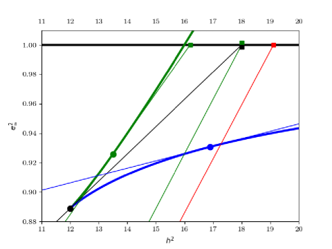
Figure 12 shows integral space for a naked black hole. When plunging orbits are allowed, the inequality (11.32):
| (11.44) |
forms in integral space a right-angled triangular region bounded by
-
i
the line , or in the integral (11.3.2) (not shown for clarity)
-
ii
the line , or in the integral (11.3.2). We do not consider the unbound orbits .
-
iii
the line (11.44), with the equality sign. This is the hypotenuse of the triangle, representing the orbits in that have zero radial velocity. We call the parameter of the hypotenuse. Five of them are shown: 2 green ones, one red, one black and one blue.
-
•
These hypotenuses intersect the vertical in , or in the integral (11.3.2). As already indicated, these are orbits with zero angular momentum, thus radial orbits, with as apocenter. The test particle is momentarily at rest. The intersection is a monotonically increasing function of .
-
•
The intersection of the hypothenuse with the line at is the marginally bound orbit for which is the pericenter. It has the largest local energy of all orbits on the hypotenuse. It is indicated by a square. In the Schwarzschild case, which is the case shown, the squares are at . The blue square is not shown for clarity (it would be at ).
In general, the local energy of the orbits on a hypotenuse increases ’from left to right’.
-
•
11.3.4 The integral subspace of non-plunging orbits
The two branches
Equation (11.44) defines 3 families of hypotenuses in integral space, depending on whether one chooses radii in an interval in which the effective potential curves have a minimum, a maximum, or no extremum. Equation (11.44) together with (11.36), which determines the extremum of , form the equations of an envelope that can be split in 2 branches. The dots in figure 12 show the location where the depicted family member touches the envelope.
-
•
The blue family, for , generates the concave blue branch, corresponding to the minima. The position of the squares increasing monotonously with .
-
•
The green family, for , generates the (slightly) convex green branch corresponding to the maxima. The green family shows a more complicated behavior. In the Schwarzschild case the position of the green squares decreases from at till at , which happens to be also the intersection of the line with the green envelope. In the sequel we will meet that radius again. For the position of the green square increases, thus reversing trend, to end up again at for . That family member is shown in the picture and has no dot, because it touches the green envelope at infinity, being the asymptote of the green branch.
-
•
The red family, for , does not form branches for . The position of the red squares continues the trend set by the green squares, and increases dramatically with decreasing , up to the limit towards infinity for , where the limit hypotenuse of the red family of zero velocity curves is . This also means a dramatic increase in accessible integral space. We have already seen that all orbits inside the sphere are plunging. Therefore the red family does not concern us here. A point on a red line of course is a zero radial velocity orbit at that radius, but they all have their apocenter at that radius. They differ by the number of windings needed to complete the plunge. This number increases with increasing .
The radius that is common to both families defines and corresponds to that unique for which the maximum and the minimum of coincide. In figure 12 (naked black hole) . The zero radial velocity line and the cusp corresponding to the common member are shown in black. The corresponding angular momentum we denote by . In the Schwarzschild case and .
Characterization of the branches
We first notice that, because of (11.32) and (11.42), that
| (11.45) |
and therefore no perturbation for fixed will violate (11.44).
The blue branch is, just as in the Newtonian case, the locus of all (stable) circular orbits. We recall from the Newtonian case that the circular orbit with radius divides the tangent line with parameter in ‘the lower half’, which represents orbits for which is the apocenter, and ‘the upper half’, representing the orbits for which is a pericenter.
In order that an orbit is a non-plunging one, we learn from figure 11 that must be smaller than the maximum of for finite , that therefore must be present. We denote that maximum by , as we did in the Schwarzschild case in section 10. The equation is the equation of the green envelope in figure 12. Hence
| (11.46) |
At radii where the equality holds, we are in a pericenter or apocenter of the orbit, since, according to (11.32), the radial velocity is zero there. For the specific combination for which , such as indicated in figure 12 by the green dot, we have an orbit that has just enough angular momentum to be a non-plunging orbit. Referring to figure 11, the radius where the effective potential curve touches the line is the pericenter of that orbit. We call such an orbit one with an unstable pericenter. For somewhat different energy or angular momentum, this orbit could flip into an orbit with that radius as (stable) pericenter or a plunging orbit with that radius as apocenter.282828These orbits are also called unstable circular orbits. For all practical purposes, this is a misnomer, since an additional force would be required to keep the orbit at fixed .
All non-plunging orbits therefore are located within the wedge formed by the blue and green branches. In topological terms, this wedge is a set that is neither open nor closed. The green branch forms an open part of the boundary, the blue branch is the closed part of the boundary.
Characterization of the orbits between the branches
Out of a given point representing an non-plunging orbit, one can always draw a tangent (the ‘upper one’) to the blue branch. The parameter of that line is the apocenter of the orbit.
As for the pericenter, there are 2 possibilities.
-
i
The point has another tangent (the ‘lower one’) to the blue branch, the parameter of which is the pericenter of the orbit. For this to be the case, the orbit must lie ’to the right’ of the black hypotenuse.
-
ii
The point has a ’lower’ tangent to the green branch, the parameter of which is again the pericenter of the orbit. For this to be the case, the orbit must lie ’to the left’ of the black hypotenuse. The black hypotenuse thus divides the 2 cases. Orbits ’to the left’ of the black hypotenuse have no ’upper’ tangent to the green branch.
The black dot is the unstable circular orbit. All non-plunging orbits are located between the 2 branches.
11.3.5 The integration over
The condition (11.46) on in order to prevent a particle from falling into the black hole assumes and as a given. However, what we need in the integration (11.3.2) is the condition on given and . To that end, we note that the function is an increasing function of , which follows from the form (11.33) of . Hence we can calculate the minimum for a given , in order to have a non-plunging orbit, being an orbit with unstable pericenter, and we denote that minimum by . The specific combination mentioned above can thus be denoted by and is again the equation of the green envelope. The condition we impose is therefore in essence a lower limit on the angular momentum, and thus, with given , we deal with a lower limit on the tangential component of the linear momentum:
| (11.47) |
In the Schwarzschild case, it is implicitly given by the inversion for of (10.9) for , and explicitly given by expression (10.10). In the present case, we need to solve (11.36), which we write as
| (11.48) |
and (11.33)
| (11.49) |
for and . The function appears here as an explicit parameter representation (in function of the parameter ), if only we knew , and . Fortunately, the radius at which the curve attains it maximum is always smaller or equal than the for which we are calculating the response, lest we be on a plunging orbit. Since we will calculate the response via the system of differential equations (11.6) and (11.12) or (11.14) from the inside out, we can tabulate as we integrate along (see also later).
11.3.6 The integration over
For the sequel we will need to ascertain whether is smaller or larger that . In the numerical calculations, we will therefore check the sign of the derivative of (11.36), which can be done by checking the (sign of the) derivative of the function
| (11.50) |
which has, obviously, the same sign as the derivative of (11.36). It serves the same function as (10.7). The zero of the derivative of (11.50) will thus mark the radius where the extrema of coincide. Hence that radius is also .
We now place ourselves at some , and visualize the curves for increasing , starting from . Initially, the maxima will be smaller than giving rise to plunging orbits. The first marginally non-plunging orbit, i.e. the orbit that has just enough angular momentum to realize a non-zero pericenter, is the one for which , and for larger than this limit value we can realize an integration interval in of non-plunging orbits since
| (11.51) |
We recognize the same condition as (11.46), on which we based our analysis of the interval. Hence the lower limit for , which we denoted by in (11.3.2), follows from the solution for of
| (11.52) |
This condition depends only on , and , since (11.52) solves for . Denoting the solution , we find
| (11.53) |
The orbit with is in figure 12 the intersection of a blue zero radial velocity line with parameter and the green envelope, and also the lower left corner of the region of integral space accessible to (non-plunging orbits). For that orbit the radius is an apocenter. The pericenter is the unstable radius . It is the same orbit that constitutes the lower bound of the integration in for that energy . In the figure, could be constructed by determining the green zero radial velocity curve that is tangent at and ascertaining its radius. For , and for we have the unstable circular orbit at , which is actually the unstable limit of a plunging orbit with apocenter .
Our second case is . For a non-plunging orbit and the expression (11.36) for is negative. Hence we need the condition
| (11.54) |
which means that we are on the ’downward’ branch of . This condition only depends on , and , and not on . The tangential momentum is thus the minimum tangential momentum the orbit must have. The corresponding is such that has a maximum at . Also in this case, it implies a minimum energy. This energy is , with , by virtue of (11.54). Hence the horizontal line with that is the tangent at the maximum of , which is at ; smaller would give rise to plunging orbits, smaller energies preclude motion. This unique orbit has and , yielding thus a minimum energy . It is an orbit with an unstable pericenter . In figure 12 it is the energy of the green dot on the green zero radial velocity curve with parameter . Angular momenta that are smaller than the angular momentum of the green dot give rise to plunging orbits. Like the blue dots, the green dots divide the tangent into 2 parts. The upper part are orbits with pericenter and an apocenter that increases if we approach . The lower part (not very well visible in the figure because the curvature of the green envelope is small) do not represent orbits at , because they are below the tangent that is the zero radial velocity curve. When , the apocenter of the orbit of which is the pericenter tends towards , yielding in the limit the unstable circular orbit.
During the calculation of the solution from the inside out, the tracing of is thus a similar process as the tracing of .
11.3.7 The moments of the distribution function
Having established the integration limits in (11.3.2), we can now perform the integration over :
with
| (11.56) |
and given by (11.47).
The radial pressure is obtained via the expression:
| (11.58) |
with the number density. Taking into account that
| (11.59) |
we have
| (11.60) |
Thus we can calculate the radial pressure by multiplying the inner integrand in (11.3.2) by or, after integration, the remaining integrand in (11.3.7) by
| (11.61) |
yielding
The tangential pressures are the same in any tangential direction, and we have
| (11.63) |
A similar calculation as above yields
This is not the same expression as for the radial pressure, since we eliminated plunging orbits. If we would not do that, , and the 3 pressures would be equal, as should for an isotropic distribution function. Clearly .
11.3.8 The central regions
The inner boundary
Obviously all the above integrals will be zero if . Therefore must satisfy
| (11.65) |
Since inside that radius, there are no bound orbiting masses, we can use the Schwarzschild case , as follows from (10.7) or (11.54) with . We recall from section 11.2 that, when integrating equations (11.6) and (11.12) from the inside out, we start with two free parameters which could be taken as and . Here our insistence on bound orbits expressed by (11.65) and the explicit expression for as given by (11.29) produces a relation between and (or ):
| (11.66) |
As we noted following (11.14), and thus . The metric coefficient , already calculated in (11.29) can be written in terms of the only parameter that remains:
| (11.67) |
We now determine the characteristics of that particular orbit with pericenter . The tangential component of the linear momentum there equals
| (11.68) |
and the angular momentum equals
| (11.69) |
By construction, , since the integration interval collapses at for . Hence the apocenter of the orbit is , where the velocity is zero. We find
| (11.70) |
The (tangential) velocity at pericenter equals, with the expressions (11.40),
| (11.71) |
All the above equations and considerations involving impose the limits
| (11.72) |
The equality signs pertain to the naked black hole.
Since the maximum of the effective potential touches , is also the minimum angular momentum a marginally bound orbit should have in order to remain in orbit around the black hole. In the Schwarzschild case, this normalized specific angular momentum equals and the critical pericenter (see also fig. 11). If mass distributions are added, increases, indicating that the added mass ’sucks’ test orbits into the abyss. Interestingly, when the depth of the potential well , which is its maximum value, .
The central response
It is instructive to establish the behaviour of and for , which can be done analytically since the integration interval collapses there. The analysis is a bit more complicated than meets the eye in (11.3.7) and (11.3.7), though.
We start by noting that all energies that are permissible for non-plunging orbits are the maximum of a unique effective potential curve . We can therefore consider the transformation from to the radius which is the radius at which the effective potential curve attains its maximum. For the radii we are in the Schwarzschild case, and thus, with (11.54)
| (11.73) |
From these expressions it is reasonable to expect that the transformation from to may result in a simplification. The maximum of is its value in :
| (11.74) |
This equation defines the transformation from to . The transformation is a decreasing one. The inverse transformation can be made explicit with (11.67) and results in a quadratic equation with solution
| (11.75) |
For the local energy we find
| (11.76) |
The lower limit in the integral over equals
| (11.77) |
If we compare this expression with (11.76) we see that the upper limit in the integral for equals . This can be verified using (11.75) if we observe that
| (11.78) |
and hence
| (11.79) |
The upper limit in the integral over equals 1, or
| (11.80) |
Insertion into (11.75) yields, quite elegantly, for the lower limit of the integral over the value .
The radicand in the integrals such as (11.3.7) transforms, after some rather lucky factorization, into
| (11.81) |
The term in reflects the fact that when then . The transformation being a decreasing one, hence , and
| (11.82) |
This allows us to write down the square root:
| (11.83) |
Lastly, the Jacobian of the transformation from to equals
| (11.84) |
Collecting all the elements so far, we obtain finally for (11.3.7):
| (11.85) | |||||
The transformation that yields the above form is valid for , as long as does not differ significantly from the expression for empty space (11.67).
In a similar way we obtain for the radial pressure
| (11.86) | |||||
The analysis can be generalized for general and for , but we will not pursue this any further. Our main purpose is to study the limit . We find
| (11.87) |
with
| (11.88) |
Similarly
| (11.89) |
with
| (11.90) |
For the mean velocity we find
| (11.91) |
which we already knew from the characteristic (11.71) of the unique orbit at for which .
Since both and tend to 0 for , we can integrate the system (11.6) and (11.12) there with a series expansion. We find
| (11.92) |
with and
| (11.93) |
with
| (11.94) |
In the expressions above it is, of course, understood that the nonlinear terms in are zero if . The linear terms in (11.93) are compliant with (11.67), since we obtain here
| (11.95) |
11.3.9 Application
We will now apply the formalism to dark matter particles that obey a Fermi-Dirac distribution. The rationale for this is that we know, from the flat rotation curves, that at least some dark matter obeys such a distribution (or a Maxwell-Boltzmann distribution).
We will express our results in terms of a reference mass eV (which is to be considered as an effective mean of the masses of all the dark matter species and their antiparticles) and a reference temperature of . The Fermi-Dirac and Boltzmann distributions also feature . Assuming km/s as a unit of velocity, this yields
| (11.96) |
The actual value of this parameter we will denote by
| (11.97) |
with reflecting our ignorance about the appropriate value of the quotient . We define
| (11.98) |
and note that
| (11.99) |
With these definitions, we obtain
| (11.100) |
featuring Planck’s constant h and the number of dark matter species . The normalisation respects the Pauli principle, i.e. should be smaller than the minimum for non-plunging orbits. In the case of a naked Schwarzschild black hole that energy equals (see fig. 11). In the general case, the minimum energy possible for a non-plunging orbit is , which is realized by the marginally bound orbit with the unstable pericenter . Hence
| (11.101) |
The equality would mean that the dark matter distribution in phase space is totally degenerate on the unstable circular orbit (with radius ).
We obtain for :
The number density is of course similar:
The radial pressure reads:
The coefficient in front of (11.3.9) simply equals the coefficient in front of (11.3.9) divided by 3. The expression for the tangential pressures follows from (11.3.7) and (11.3.9), mutatis mutandis in the integrand.
11.3.10 Some examples and discussion
As already indicated below equation (11.9), the density (11.3.9) and the pressure (11.3.9) are determined by integrating the system (11.6) and (11.12) over with the initial conditions and . Since everywhere, there is no clear recipe for determining the outer boundary . It will depend on the mass of the black hole, the formation process, the amount of dark matter available and temperature of the dark matter particles.292929The outward integration we use here is of course not a reflection of what would have happened physically. The collapse and accretion processes would have run their courses, and in the end would have followed from that, much like, classically, the mass density comes first, and the central potential follows from (11.108)
The solution clearly depends on parameters. There are the 3 scaling parameters: average mass of the dark matter particle , number of degrees of freedom and geometrical mass of the black hole . The other 3 are the temperature , normalisation and the depth of the potential well . The outer boundary is to some extent also a free parameter.
In the assumption that is largely determined by the mass of the surrounding galaxy, we can obtain a relation involving and the mass of the galaxy. Assuming a simple Hernquist potential
| (11.109) |
we find
| (11.110) |
since is much larger than near the black hole. This approximation is probably valid for many more potentials for which it makes sense to define a ‘mean’ radius . If the dynamical effects of the stellar mass in the close vicinity of the black hole is negligible compared to these of the mass of the black hole, we can match the linear terms in (11.93) with the above expression to obtain at the match point
| (11.111) |
This radius should be larger than , leading to
| (11.112) |
which is hardly a constraint since the above expression translates into the requirement that the scaling radius of the galaxy, expressed in Schwarzschild radii of the galaxy, should be larger than .
If , equation (11.111) has the solution and . For very deep potential wells, the expression (11.109) should be replaced by a general relativistic one. Assuming that in reality it is never really necessary to recur to general relativity for galaxy dynamics, the (unattainable) limit would lead to which means that would be equal to the Schwarzschild radius of the mass of the galaxy as a whole. Physically this makes sense, but it is quite impossible in the present state of the universe. It might be considered as a possibility though in the dense phases of the history of our universe.
We don’t see the usual dependence on for the density or for the pressure. This is a result from the integration, which is only over a small range in , whereas usually one integrates from to .303030In the latter case, a substitution would be in order, leading to the temperature dependence just mentioned. As a consequence, for values of and such that , the part of the neutrino distribution that we integrate over is completely degenerate.
The figures are models for the dark matter envelope of the black hole at the center of the Milky Way. For a discussion, we refer to the captions.
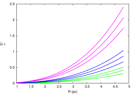
11.4 Neutrino dark matter distributions in galaxies
11.4.1 On the formation of the neutrino halo
Any model for dark matter must be able to produce flat rotation curves. A necessary and sufficient condition in a spherical geometry is that the total mass enclosed within a certain radius increases roughly linearly with that radius. If that mass obeys collisionless dynamics, there are many equilibrium anisotropic distribution functions (functions of energy and the magnitude of the angular momentum) that would qualify. However, if the full freedom of anisotropic distribution functions is to be allowed, it seems unlikely that in all cases they would ’end up’ producing flat rotation curves. For the subset of isotropic distribution functions on the contrary, a necessary and sufficient configuration is the (approximately) selfconsistent isothermal sphere, which, if fully selfconsistent without other mass distributions, depends on only one parameter, the temperature.
There is at least one more inference that must be made in connection with flat rotation curves: if the dark matter is isothermal, it must also be one phase, i.e. it is not a superposition of isothermal distributions with different temperatures. Of course, it cannot be excluded that neutrino’s exist in different phases with different temperatures. Since the temperature drops with the expansion of the universe, at a certain epoch a treshold must have been attained at which the coldest of the neutrino phases that are abundant enough to yield a dynamically significant dark matter component and that happened to be in the neighbourhood of a galaxy became ’trapped’ or ’locked’ into the gravitational field of the galaxy in a relatively short period of time (compared with the timescale of the expansion phase, of course). Note also that the neutrino’s have always been in equilibrium around the galaxy, only at (and later) the coldest dynamically significant phase becomes for the most part bound.
We note also that, because isothermal distributions are the only isotropic distribution functions that produce flat rotation curves,313131Assuming sphericity. Any departure of sphericity is not likely to change the qualitative arguments in this section. the functional form of the distribution clearly must remain approximately constant during halo formation. This means that, in virtue of Jeans’s theorem, the halo formation must have been sufficiently fast, lest the galaxy’s gravity impinge too much on the form of the distribution function.
This scenario yields a constraint. A flat rotation curve can only be obtained if the mass density is close to an exponential of the potential. If the distribution is to be bound, the expression of the mass density (F.22) shows that the argument must be large enough in order that the normalized incomplete gamma function is close to 1. This is the case if
| (11.113) |
with the mass of the galaxy and the neutrino’s combined inside the radii where the rotation curve is flat. In terms of , as defined in (11.97), we obtain
| (11.114) |
For a selfconsistent isothermal distribution the constant circular velocity equals
| (11.115) |
and thus
| (11.116) |
All these inequalities seem to be consistent with the observations. If we adopt as a representative value we obtain . This may seem like a large number (hence large average neutrino mass or very cold neutrino distribution, or a combination of both), but it is simply an observational fact, and it satisfies the constraint (11.114) for, say, a Milky Way like galaxy. Therefore this order of magnitude for is not a consequence of the paradigm we adopted for this paper, but must be explained by any dark matter candidate. If eV as suggested in fig. 16, then K.
Condition (11.116) assures that, if the mass in neutrino’s dominates the stellar mass, the neutrino mass density essentially follows the well-known isothermal sphere law
| (11.117) |
clearly showing the direct relation between and the amount of dark matter. Hence neutrino’s in circular orbits will have the same velocities as stars and gas in circular orbits.
On the other hand, inspection of figure 5 or 6 reveals that between ’lock-in’ time and the current epoch, the radius of our universe, as defined in (6.9), has increased by a rather modest one digit factor, presumably larger than 3. Assuming the standard relation
| (11.118) |
the neutrino temperature now can be estimated as a factor of 10-50 smaller than at ’lock-in’ time.
At , in addition, the cosmic deceleration should be less than the gravitational attraction of the galaxy, so that the neutrino’s, which were at temperature , would not continue to cool appreciably, lest a temperature gradient occur which we don’t see. As a consequence, the cosmic evolution stops being important for these neutrinos, and they become a gravitationally bound distribution, in equilibrium around the galaxy.
In order to treat this condition semi-quantitatively, we note that for any material particle that freely moves (i.e. on a geodesic, but not necessarily comoving and in the absence of an appreciable gravitational field) with velocity with respect to a comoving observer at the same location in a synchronous universe (on the scales of galaxy clusters this is a good approximation) is a constant. This means that
| (11.119) |
The cosmic deceleration therefore acts as a kind of friction that is proportional to the velocity . The attraction due to the galaxy must be considerably larger than this frictional force, and hence
| (11.120) |
with a characteristic size, a characteristic velocity of the neutrino distribution and a dimensionless fudge factor. This factor stands for all the unknowns, is presumably somewhere in the one digit range, but probably larger than 5, meaning that the cosmic deceleration is only between and of the galactic attraction. For an isothermal distribution
| (11.121) |
and thus
| (11.122) |
or, with ,
| (11.123) |
If we insert , and we obtain , or in our units . Referring to the figures 5 and 6 that show models for which occurs at after the beginning of the latest expansion phase, we see that the ’lock-in’ time must have occurred before the universe was far in that latest expansion phase. Given the great uncertainties in this qualitative argument, it is also possible that the neutrino’s were already locked up when the latest expansion phase commenced.
Any more detailed analysis of this ’trapping’ of neutrino’s by galaxies would require a large cosmological scale simulation with many clusters, galaxies and neutrino clouds, thereby forgoing the fact that, in our paradigm, the initial conditions for such a simulation are basically unknown anyway.
11.4.2 A simple model for a Milky Way type galaxy
The neutrino density at infinity will be expressed as a factor of the standard closure density (see equation (2.7) and the comment there) and we write
| (11.124) |
according to (2.8), with reflecting our uncertainty as to the value of the background neutrino density at ’lock-in’ time.
As argued above, we assume that the neutrino’s are bound to the galaxy, and therefore we adopt the halo density (F.22). The essential ingredient for flat rotation curves is a central mass concentration. The reason is that the signature of the exponential in (F.22) must be present, which is only the case if the potential well is deep enough in order that a sufficient number of neutrino’s are bound. Therefore a bulge-like structure must be present if we are to obtain a flat rotation curve. This is consistent with the bulges being old. They may be formed, together with the globulars, in an era preceding the latest expansion phase. Denoting the mass density of the galaxy, excluding the dark matter, by , we look for an equilibrium configuration that can be found by solving the spherical Poisson equation. It is clear that, because of the assumption of sphericity, we do not need to aim for much detail, and the model therefore is not much more than a proof of concept.
In this subsection we adopt 1 Mpc as the unit of distance, express masses in the unit and keep km/s as the unit of velocity. The neutrino density at infinity is then
| (11.125) |
Thus we obtain the form of the Poisson equation that we are to integrate:
with
| (11.127) |
the Newtonian binding potential, and the mass in stars and dust, including the central mass concentration.
We will treat (11.4.2) as an initial value problem and we integrate outwards, and thus we need and . From the previous subsection, we know that the mass density is essentially constant around the central black hole. Therefore, we can start the integration at about 5 pc ( in our units), and an enclosed mass of ( in our units), which is presumably an underestimate. The potential is quadratic, the coefficient of is fixed by the choices above, but we can still choose . It turns out that is not a bad choice.
For we adopt a Hernquist bulge and an exponential envelope
| (11.128) |
with , (Widrow & Dubinsky [17]), (rather arbitrary) and (from fig. 15 in Fathi et.al. [18]). The integration is stopped when the total mass in neutrino’s equals the total mass in a constant density sphere with density , indicating that the neutrino’s have settled in a selfconsistent distribution.

12 Dark energy
The case for dark energy rests essentially on 3 arguments: the occurrence of a big bang and the consequences that come with it (such as the nucleosynthesis of light elements), the magnitude-redshift relation and the analysis of the CMB. In our paradigm, the first argument is powerless, since there is no such thing as a big bang ’of creation’ (section 5.2). As to the second argument, it is very plausible from subsection 9.6 that the and relations can be satisfied by our models, even with . If needed, we can invoke which has the same effect as the dark energy, but that choice is then to be a feature of the ’mother universe’ that our universe contains, and of which all knowledge is futile anyway. In general, one is not used to consider black holes with a . The main characteristics of them are touched upon in appendix B.1. Lastly, the universes we consider have a CMB that is isotropic by design, and if it contains fluctuations, they cannot learn us very much because they are the remnants of details of history that do not change the grand picture.
13 Mach’s principle and Newton’s second law
Mach’s principle is rooted in a discussion that dates back to Newton and Leibniz. To the latter, space was simply a construct which was useful to stage the introduction of coordinates, and he correctly realized that the actual choice of the coordinates is quite arbitrary. Hence, any physical theory should be independent of the choice of a coordinate system, and therefore he was an advocate of covariance avant la lettre. Newton on the other hand quite convincingly proved Leibniz ’wrong’ with his famous pail experiment, showing that one must endow the concept of ’absolute space’ with physical reality.
Here, just as in conventional cosmology, it is quite natural to promote the comoving frame to the status of coordinated absolute space, and since comoving observers do not experience any accelerations, the special significance of their coordinate systems does right to the special significance of absolute space.
The above statement does not explain, however, what the physical mechanisms are behind the ’punishments’ that inhabitants of coordinate frames that are not comoving must endure, such as the so called ’apparent forces’ (linear acceleration, centrifugal and Coriolis forces). These forces are proportional to mass, but they have nothing to do with gravitation. Hence the need for inertial mass as distinct from the gravitational mass . Mach’s idea is simple and attractive: it is the whole body of the universe that defines the absolute frame. Yet, a physical explanation to back up the idea is not part of Mach’s principle, and as such Mach’s principle is therefore ’nothing more’ than the assertion in the previous paragraph. It does suggest, however, a link between and .
General relativity evades the issue, in a sense. It replaces Newton’s second law with the geodetic equations. These deal with accelerations, not with forces. Hence there is no need to introduce . This also means that we cannot use general relativity as a tool to investigate Mach’s principle.
We now revisit Mach’s principle in the framework of our universes. We invoke a cosmic (dark) matter background . It has been argued in section 11.1 that it is very likely to be highly isotropic, and thus . The attraction of that isotropic background on a mass causes a net force that is zero, as was already known to Newton, be it that in his case the net force was the subtraction of 2 infinities. Here, however, the universes are finite in spacetime, and no singularities are to be confronted. Therefore, we can actually calculate something.
The zero net attraction causes a tension, however. A similar situation occurs if a (massless) particle is attached to two very long springs that pull at it in opposite directions with equal force, so that there is equilibrium. Because the springs are very long, Hooke’s law (typically , with the distance from the equilibrium point and the spring constant) does not apply, and the force is independent of . If we apply a force on the particle, this will cause an acceleration. The more the springs are tautened however, the smaller the acceleration will be for the same applied force. The particle thus acquires a stiffness due to the tension in the springs.
In order to obtain the tension that a massive test particle experiences, we now calculate the acceleration due to the mass density in one hemisphere. We can work in the weak field limit, and thus the law applies. However, our universes are not static. The ’distance’ between 2 massive points is set by the light travel time, since it follows from the mathematical structure of the Einstein equations that gravitation propagates along null geodesics.
In a static universe, we would obtain the tension by integration of the gravitational attraction law over one hemisphere:
| (13.1) |
Here we turn to the formalism proper to the synchronous universes of section 6.1. The metric (6.6) gives rise to the volume element at emission time of an attractor
| (13.2) |
which should replace the volume element in (13.1). The factor in the denominator of (13.1) is the Euclidean surface of the sphere centered on the attractor with coordinates on which the test particle with coordinates is located. This should be replaced by the surface area of the sphere in curved spacetime
with the angle between attractor and test particle on the great circle that connects both and that was referred to at the end of section 9.5.1. In this expression, we changed coordinate systems to put the attractor at the center and integrated over a suitable defined (the factor ) and (the factor 2). Collecting these changes and integrating over , we obtain
| (13.3) | |||||
For the case we consider here, the synchronous universes, this expression simplifies a lot. We use the explicit expressions (6.20) for and (6.3) for , and obtain
| (13.4) |
This is still a complicated integral, as it stands, but it is a purely geometrical one. We can now use the embedding paradigm which transforms the 2D universe to the surface of a sphere, be it that ‘the lower hemisphere’ is to be identified with ‘the upper hemisphere’. This allows us to see the lines of force as great circles on the surface of that sphere. Hence we can again change the coordinate system to a new one in which the test particle is at . This makes the integrand trivial, since . We can integrate over the angles
to obtain
| (13.5) |
In order to calculate the integral over , we recall from section 9.5.1 that for a closed synchronous universe with , for every observer during a full expansion or a full contraction. Two images (a direct one and a reflected one, the latter being in the opposite direction of the direct one in the case of perfect symmetry) of every object are produced during one full expansion or one full contraction. These images will not appear at the same time, of course, but within the period . The same is true for the lines of force, which are basically the same thing: there will be one direct line of force, and one reflected line of force. The integral over measures the amount of universe that contributes to the attraction.
According to (3.14) we denoted the time-lapse of a full expansion or contraction with (in our units), with for simplicity. Hence,
| (13.6) |
where we divided by in order to get explicitly a time-lapse. Thus, the integral in (13.5) increases linearly with time, and if we wait for , the integral equals :
| (13.7) |
Substitution of (13.6), (6.19):
| (13.8) |
and (6.21): into (13.5), yields
| (13.9) |
With (6.3): we end up with
| (13.10) |
Isotropy of is assured by the isotropy of the universe, which in our paradigm is a consequence of the very many cycles our universe has gone through. We argued that in that case a given mass should influence our test particle through (many) different lines of force. Hence we don’t need the restriction to one cycle anymore, and we can state
| (13.11) |
If we add to this the logically consistent hypothesis that our universe once was born as a (regular) black hole in our mother universe, of course very much longer ago than 13.6 billion years, and that it got its mass by accretion, we must also try to take these accretion events into account.
The mass of a closed synchronous universe is given by (6.16):
| (13.12) |
in which we substituted (6.19). Hence, with (13.6)
| (13.13) |
Suppose we have a number of accretion events, separated in time by intervals , . The universe is born with an initial mass at event . At accretion event a mass is added. Of course , the total mass of the universe. As for the full age of the universe,
| (13.14) |
with the time-lapse since the last accretion event, which might be of the order of what we probably would call the age of the universe.
In time-lapse between creation and the first accretion event, there were periods,323232It doesn’t matter that this number is in general not an integer, since the horizon increases linearly with time. with , each producing the number of images that are included in (13.11), and these are images of a fraction of the current total mass. In time between the first and the second accretion event, there were periods, with , each producing the number of images that are included in (13.11), and these are images of a fraction of the current total mass. Continuing that way, we find for the number of images
or
| (13.15) |
This is again a linear increase with time, and (13.11) therefore remains valid, irrespective of the accretion history:
| (13.16) | |||||
The factor that is multiplied with should be one if is to be equal to . Hence we need a truly very long age to make this work, though we should add that is relevant for our mother universe, of which we know nothing anyway.
The only constraint we have on , with the current epoch, is the (tangential) Hubble parameter . In section 3.5.3, equation (3.41), we obtained an expression for , given the parameter , here assuming and . For small (this seems imperative if (13.16) is to work) and thus large , we obtain
| (13.17) |
and hence we get for (13.11)
| (13.18) | |||||
It thus seems imperative to consider the possibility that our universe is smaller than we currently think. The phenomenon that a universe has a boundary, functioning as a gravitational mirror (section 8.2.2), which is a novel concept introduced in this paper, could certainly cause us to interpret certain objects as being far away that are in reality images in reflection off the boundary. There would be no way to ascertain the presence of the boundary, unless both images would appear to collide. It would be non-trivial however to identify objects ‘in direct view’ and ‘in reflection’, since these views would be at different aspect angles and (much) different ages. Be it as it may, for , which is still larger than the size of typical galaxy clusters, it is possible to obtain for ‘reasonable’ ages , certainly because we have no clue what the latter should be anyway.
Another consequence of (13.11) is that for very small , which may still be huge since is expressed in , the inertial acceleration can become huge. That means that no known force except gravitation would be able to throw a massive particle off its geodesic course, not only preventing the formation of atoms, but presumably also acting as a driver in synchronizing a universe and/or keeping it that way. This could explain why our universe appears to be highly synchronized, which thus would be a relic of a very distant past, during which our universe was completely ionized but thermally cold because of the complete absence of random motions.
14 Summary
In this paper, we consider spherically symmetrical cosmological models that are the interior of black holes, for our purposes defined as the matter in the spacetime inside a Schwarzschild horizon.
By virtue of the spherical symmetry, the universe can be ordered in spherical shells, which are given a label which is not a radius, but these labels preserve order with the surface area of the shells. The labels are time independent, in contrast with the surface area (subsection 2.1).
We employ the well-known Lemaître-Tolman models (section 2), but recast them in a form that suits our purposes. More in particular, we introduce in subsection 3.1 the function ’cyc’, which is a generalization of the well known cycloidal solution of the Robertson-Walker (RW) models. We study it extensively in appendix A. This function not only packs all technical mathematical details of the time evolution equation into one mathematical object, thereby formally separating all mathematical details from the essence of the physics, but its introduction is also almost necessary in order to deal elegantly with the complications that arise from the spherical symmetry. In subsection 3.6 we briefly show how ’cyc’ connects with the standard practices in cosmology and the parameters of the ’concordance’ CDM model.
We present the view that, in order to understand the current state of our universe, it is essential to consider states in the very distant past in which the universe was not in expansion. In section 5 we muse about these phases, and argue that the isotropy of the Cosmic Microwave Background can be understood as a consequence of them, in a qualitative sense that is. A big bang is still possible, but (a) how ’big’ that ’bang’ was we cannot know, (b) it is possible that there were many ’bangs’ (in space and/or time), and (c) there is no need to invoke ’bangs of creation’ or (d) to consider ’bangs’ that originate out of a ’point’ in space.
Shells can collide (subsections 3.2 and 5.1), or put differently, a universe not necessarily evolves in a synchronous way. This possibility adds an important twist to cosmological models, since RW models (these belong to a class which we call synchronous models) do not allow for collisions. Colliding shells provide a natural mechanism to make filamentary structures333333In this paper we remain in the spherical symmetry. The structures are thus spherical shells.. Collisions also mark singularities in the metric. These do not invalidate the geometrical theory of gravitation, of course, but their occurrence shows the danger in assuming that one metric can be employed, without limits in space and time, to describe the universe. We argue that there is an important difference between the validity period of a (geometrical) cosmological model and the real age of the universe. We must acknowledge that the latter may be impossible to determine, in contrast with the age of the structures in it, which can be dated. If we consider the consequences of collisions together with the ideas of the previous paragraph, one can envisage a universe as comprised of many smaller entities, somewhat like a raspberry or a pomegranate.
We consider a rather general class of specific cosmological models, but must admit, of course, that we cannot be exhaustive (subsection 6.2). Also models that have infinite extent or that are not the interiors of black holes are part of this class, but are not the subject of this paper. Barring these models, our models have an outermost shell, the boundary, beyond which there is no matter. The RW models are ’almost everywhere’ identical to the synchronous models (subsection 6.1), the exception being that they differ from these on the boundary, which the RW models simply don’t have.
The Hubble parameter is dependent on the viewing direction, and we define to be the current value as measured in the direction perpendicular to the center of the universe. This definition is consistent with the original definition in the standard cosmological models. We consider only models that realise somewhere and sometime (subsection 3.5), and classify them in some loose sense accordingly (subsection 6.2). In subsection 6.3 we also consider another, rather technical, classification that has to do with the behaviour of the radial metric coefficient at the boundary. It is important in the calculation of orbits.
Contrary to the standard models, we have to cope with planar orbits instead of radial orbits, which is the subject of section 8. We devote a special section (section 9) to light, since it can be argued that photons are the only particles that are essentially not comoving and thus can be considered to be traveling on a cosmological scale. In subsection 8.2 we examine the behaviour of the orbits in the vicinity of the boundary. We show that no particle can cross the boundary. Upon arrival they are reflected back into the universe. The boundary therefore effectively acts as a gravitational mirror. Unlike an ordinary mirror, however, one effectively flies into the mirror image upon arrival at the boundary, causing a spinor-like effect. This mirror-boundary could have far-reaching consequences. To pick one, it could be that our universe looks larger than it is. Indeed, we may find ourselves as if we were inside a spherical mirror. For that mirror to have effective observational consequences one needs (light travel) time, however (and transparent space of course). We discuss this and other rather intriguing aspects of the boundary in subsection 8.2.2.
If our universe is confined inside a Schwarzschild horizon, we must also consider ’the mother universe’. In particular, we must consider material that falls into our universe from there. The connection between the Schwarzschild- metric of our mother universe and the metric of our universe is elucidated in appendix B. We employ Novikov coordinates, which are the coordinates of an observer who moves in a swarm of radially infalling shells, and who determines his radial position by the shell that passes by. These coordinates give rise to a diagonal metric, but are nevertheless largely unused because of the metric coefficients which are fairly complicated in their original form. The function ’cyc’ however hides the mathematical details, and the resulting metric turns out, in hindsight not surprisingly, to be of the form of the metric of our universe, but it is one that is, in contrast, collapsing. Additional great features of the Novikov coordinates are that they can be easily interpreted and there is no horizon singularity. Hence it is possible to treat the infalling particle problem, since spacetime is not treated differently inside or outside the Schwarzschild radius. This is outlined in section 4, with the aid of the formalism developed in subsection B.4.
In section 4 we also discriminate between the Schwarzschild sphere of the universe and the boundary of the universe. The picture emerges, at least in the ideal spherical and ordered case without colliding shells, of a kind of ’breathing’ universe in the spacetime that does not belong to the universe and that is ’interior’ to the Schwarzschild radius.343434Strictly spoken, there should be nothing left between the edge of the universe and its Schwarzschild radius, but we keep the possibility open that, with the help of non-spherical evolutions in the past, there are some leftovers from a previous expansion phase. In any case, whatever there is, it continuously falls back into the universe. The maximum expansion of the universe occurs at the very moment when also the universe fills its Schwarzschild sphere. At all other times, it does not, and there is (empty) space-time between the boundary of the universe and the Schwarzschild horizon, space-time that can be described with a Novikov metric. In this picture, it therefore is not correct to ascertain that an expanding universe ’creates’ space along with its expansion. Our universes simply expand into the preexisting space-time interior to their Schwarzschild spheres.
The above picture also points to an intriguing possibility that can occur when a black hole with a universe inside is in a state in which its universe reaches the Schwarzschild radius. In section 7.2 we show that, if at that very moment of maximum expansion the shells at the boundary also collide, it is possible that the boundary, and hence the Schwarzschild shell, is crossed from the inside to the outside. Unlikely as this may be globally, it could be realized locally (thereby breaking the spherical symmetry of course). This could be relevant for ’ordinary’ black holes, which are most likely rotating and described by a Kerr metric. This metric however is locally, at the poles, similar to the Schwarzschild metric, and therefore emission at the poles could be a possibility, thereby enabling bipolar outflows.
In section 7.3 we link this mechanism also to H. Arp’s anomalous redshifts, since material that manages to escape from a black hole must climb out of a rather formidable gravitational well. Barring the cases of chance alignments, the anomalous redshifts are therefore not cosmological but gravitational according to this mechanism.353535We do not advocate that all Arp’s cases are of this nature. Surely there can be chance alignments. Hence statistics on Arp’s catalog is not very relevant to the point made in this paper.
In standard cosmologies, any point can be the center of the universe, any light ray can therefore be a radial one, and flux calculations are straightforward by considering the surface of a sphere centered at the origin. Not so in this case, and in appendices D and E we set up the necessary machinery to calculate the magnitude as a function of redshift (section 9), which is needed to fit models with observations. We find, of course, that the relation depends on the direction of the line-of-sight. Though a fit to observations is way beyond the scope of this paper, we show in section 9.6 that the presence of a phase function suffices to fit current observations without having to invoke dark energy. We also compare some of our models with the consensus model, and find that we can reproduce it, of course, but also with .363636Since this paper includes the case and RW models are part of the class we consider (almost everywhere), a satisfying fit to observations is a trivial matter anyway.
In section 12 we briefly comment on dark energy. Since dark energy and are essentially the same thing observationally, in our models a is a property of the mother universe, of which we never will know anything except via whatever falls from there into our universe.
In section 10 we speculate about the formation of galaxies. Not much more can be done, since our models have a history before the latest expansion phase that we are in now. We argue that in our paradigm one should seriously consider that at least some black holes are primordial to our expansion phase, either by infall from our mother universe, or by growth in a collapse phase. Indeed, we show that black holes can easily gobble up a lot of material if the collapse around it is strong enough. The well-established relation between central black holes and the mass of the halo for spiral galaxies suggests that at least spirals are basically giant accretion disks around massive black holes, formed in a (local) collapse phase. The picture of our universe as a black hole in a mother universe, together with our universe comprising numerous super massive black holes that are the seeds of new universes, is logically consistent and therefore rather appealing.
As to the dark matter, in section 11 we pick up the old idea that it is made up of neutrino’s, but stress that the analysis is valid for any particle that obeys a Fermi-Dirac or Boltzmann distribution. For this to work, the dark matter must be massive enough, cold enough, and dense enough, all of which are problematic properties in standard cosmology because they would close the universe. Not here, on the contrary: our models are closed by design. We show in section 11.3 that the remnant of a gravitational collapse that forms or grows a primordial black hole is a nearly constant density sphere of trapped dark matter particles. For a Milky Way type black hole, that sphere easily may contain as much mass as the black hole itself within about 5 pc, which is not contrary to observations of our Milky Way black hole environment. For larger black holes, the dark matter envelope can be very massive depending on its extent, and therefore the inferred black hole masses can include a very important contribution from the dark matter envelope.
On a larger scale, the flat rotation curves of spirals show that the dark matter distribution must have been isothermal at the moment in the expansion when they were ’locked in’ into the galaxies (section 11.4.1). Just like the isotropy of the CMB, this points to the scenario that our universe must be much older than the latest expansion phase, such that it was able to also produce a isotropic and isothermal cosmic dark matter background. It should be emphasized, though, that the structures we now see need not nearly be as old. In section 11.4.2 we produce a simple spherical model which includes the essential ingredients of a Milky Way type galaxy with a flat rotation curve.
In the final section, we revisit Mach’s principle in the light of our universes. We show that inertial mass can be explained as a kind of stiffness that every massive particle acquires as a consequence of the attraction by the cosmic dark matter background.
Acknowledgments
Much of this work has been done in my free time. I would like to thank my wife Tine who has given me all the freedom to work on this paper. Comments by J. Binney on an advanced version of the paper are gratefully acknowledged. I also thank the geometer H. Van Maldeghem for his comments on the geometrical aspects of this paper.
References
- [1] Misner, C., Thorne, K., Wheeler, J.A., 1973, ”Gravitation”, W.H. Freeman
- [2] Krasinsky A., 1997, ”Inhomogeneous Cosmological Models”, Cambridge Univ. Press
- [3] Lemaître, G., 1933, Ann. Soc. Sci. Bruxelles, A53, 51
- [4] Tolman, R.C., 1934, Proc. Nat. Acad. Sci. USA, 20, 169
- [5] Bondi, H., 1947, MNRAS, 107, 410
- [6] Adler, R., Bazin, M., Schiffer, M., 1975, ”Introduction to General Relativity”, Mc Graw-Hill
- [7] Hellaby, C. and Lake, K., 1985, Astrophys. J. 290, 381 + erratum Astrophys. J. 300, 461
- [8] Iguchi, H., Nakamura, T. and Nakao, K., 2002, Progr. Theor. Phys. 108, 809
- [9] Gurzadyan, V.G., Penrose, R., 2013, Eur. Phys. J. Plus, 128, 22
- [10] Pecker, J-C, Narlikar, J, 2006, ”Current Issues in Cosmology”, Cambridge University Press
- [11] McClure, M.L., Dyer, C.C., New Astronomy, 12, 533
- [12] Baes, M., Buyle, P., Hau, G., Dejonghe, H., 2003, MNRAS, 341, L44
- [13] Paganini R., Straumann N., Wyler D., 1987, Astron. & Astroph., 177, 84
- [14] Nieuwenhuizen, Th., 2009, EPL, 86, 59001
- [15] Landau, L.D., Lifshitz, E.M., 1971, The classical theory of fields, Pergamon Press
- [16] Genzel, R., Eisenhauer, F., Gillessen, S., 2010, Rev. Mod. Phys., 82, No.4, 3121
- [17] Widrow, L, Dubinsky, J., 2005, Ap. J., 631, 838
- [18] Fathi, K., Allen, M., Boch, T., Hatziminaoglou, E., Peletier, R., 2010, MNRAS, 406, 1595
- [19] Carlson, B.C., 1988, Math. of comp., 183, 267
- [20] NIST Digital Library of Mathematical Functions, http://dlmf.nist.gov/
Appendix A The function and its associate functions
Not all material in this appendix is new. This appendix is intended to be functional for the paper, self-contained and rather complete, and it presents the mathematics of the solution of the evolution equation in a consistent manner.
A.1 Some general formulae
Equations (3.1) and (3.3) lead us to define the function through the following implicit expression:
| (A.1) |
In the case that the radicand in the denominator has (a) positive root(s), we denote the (smallest) root with and (A.1) defines the principal branch of a periodic function. Still in that case, we denote
| (A.2) |
and define
| (A.5) |
with given by (3.1), and endless repeats for . The function resembles a cycloidal function.
In the case that the radicand in the denominator of (A.1) has no positive root, , the function is monotonically increasing and .
In contrast to conventional cosmology (the synchronous cases of sections A.3 and 6.1), where only depends on , and, moreover, only enters in the time dependency of the radius of the universe, we are here faced with a function that is in addition dependent on through , end . It therefore also enters into the spatial part of the metric in a non trivial way. Hence, instead of satisfying oneself with a numerical solution of (A.1), some more analysis is needed for efficiency reasons. Since , we need to calculate partial derivatives of with respect to all three arguments, and subsequently apply the chain rule. The latter operations are cumbersome but trivial, the former are also cumbersome but less trivial.
The easy derivatives we need are those with respect to . We find
| (A.7) |
The minus sign in (A.7) applies to the downward branch of the cycloidal case. This is compatible with the left hand side in (2.23), which allows both signs for . We further need
| (A.8) |
and also
| (A.9) |
As to , we find after manipulation of (A.1),
| (A.10) |
with
| (A.11) |
This function is finite for all .
The expression needs some further manipulations. In fact, in turns out convenient to consider :
| (A.12) | |||||
The term in is needed should the phase function depend on (as is the case in appendix B).
The above expression transforms, after performing a differentiation with respect to :
| (A.13) | |||||
with
Also this function is finite for all .
The derivatives , , and are all we need to integrate orbits. For the photometry however, we need to dig deeper into the second and third derivatives.
As for the second derivatives, these are the easy ones:
| (A.15) |
and
| (A.16) |
Those with respect to and are more involved:
| (A.17) |
with
| (A.18) |
| (A.19) | |||||
with
| (A.20) |
and
| (A.21) | |||||
with
| (A.22) |
The other third derivatives we need are , , , , . These are rather trivially obtained from the above expressions, and do not generate any additional irreducible integrals.
A.2 On the numerical calculation of
In order to calculate , we need to numerically invert (A.1). Efficiency can be gained if we have an estimate. For in the vicinity of 0, we obtain
| (A.23) |
with and
This expression allows one to calculate up to and including order .
When is bounded, it is bounded by the smallest positive root of (as defined in this section, see also later). In the vicinity of , with , we find
| (A.25) |
with and
| (A.26) |
In the next subsections, we will study the integrals (A.1), (A.11), (A.1), (A.18), (A.20) and (A.22) in detail. We will consider the 3 cases , and separately, though all the integrals clearly indicate that the limit is infinitely smooth.
A.3 The case over some range in
We discuss this case first, and in some detail, because the standard CDM cosmological model belongs to this class. This case is actually a special case of the more general case A.11, but it is special because all the functions we need can be made explicit in terms of elementary functions. The solutions of (3.1) are particularly simple indeed, and they all represent Euclidean flat models at any given time. We consider only expansion.
A.3.1 and
We find
| (A.27) |
There are 2 subcases.
| (A.28) |
for , and
| (A.29) |
for . The factorization in and is one that yields a regular limit for cyc if . In the bound case, and . We note in passing that .
In these expressions, there is an implicit unit of length. This can be avoided by using the definition (3.8) of representation (b), but then and also are functions of , which is unnecessary.
The classification in section 3.5.2 for the solutions for is applicable. In order to realize , there is therefore the condition
| (A.30) |
if . The function , discussed in 3.5.3, can be calculated explicitly. We obtain
| (A.31) |
for , and
| (A.32) |
for . Whether this also corresponds to a positive depends on the phase function .
A.3.2 and
We find
| (A.33) |
This is a spherically anisotropic generalisation of the familiar Einstein - de Sitter universe. This means in particular that, though space is Euclidean at any time, expansion is not uniform, and can be described with a scale function and a phase function . This solution can also be brought in the form (3.3), adhering to the definition of in (3.5), and we find
| (A.34) |
with arbitrary. Clearly this case is the limit of the previous cases , and therefore we can as well adopt (A.27).
A.3.3
In empty space must be positive or zero, and one obtains the anisotropic generalisation of the de Sitter universe, which is described, after an appropriate shell label transformation, as
| (A.37) |
with an arbitrary scale factor with the dimension of a length. We have and . Euclidean space has .
A.3.4 Discussion
We see that, in all these models, is a separable function of and if the phase function is a constant. Hence we can relabel such that (see also section 6.1 for the meaning of this choice). The non-trivial dependence of these models on therefore solely resides in the phase function . Shells will not intersect if shells with smaller start their expansion later, which means that .
A.4 The case and
This case demands a separate treatment, because there is only 1 root in the denominator of (A.1).
A.4.1 The case
In this case the integration in (A.1) is bounded by the root of the denominator. We obtain the well known
| (A.38) |
It defines the familiar cycloidal function which rises from 0 to in the interval , and declines from to 0 in the interval . Clearly . We recover (A.34) in the limit . The familiar parametric representation of the cycloid is recovered by setting
| (A.39) |
leading to
| (A.40) |
We also need
and
| (A.42) |
with
| (A.43) |
For small the above expressions need power expansions in for numerical stability.
A.4.2 The case
The function is unbounded, and is implicitly given by the elementary integral
| (A.44) |
Again, a perhaps more familiar parametric form is
| (A.45) |
leading to
| (A.46) |
As for and , we obtain quite analogously as in the previous case
| (A.47) | |||||
| (A.48) |
with
| (A.49) | |||||
A.5 The case or with
A.6 The roots of the cubic
The roots of the denominator in (A.1) are real. One of them is negative, which we denote by , the other 2 are positive and are denoted by and , with . Hence, is bounded by . Since the cubic is already in the Cardano form, we know that . We find
| (A.50) |
and
| (A.51) |
for .
It is instructive to investigate the structure of the roots in both limits. When , we write
| (A.52) |
with
| (A.53) |
we find
| (A.54) |
| (A.55) |
and
| (A.56) |
In the other limit we find and . One can also prove that in this case,373737 For any root (A.57) For this expression is positive for . Hence is increasing and remains positive up to the limit where . and therefore is to be found in the interval .
A.7 The integral for
Turning to the integral (A.1), we find, with the transformation
| (A.58) |
that
with
| (A.60) |
or, in Carlson’s ([19]) notation,
| (A.61) |
In this expression, denotes Carlson’s elliptic integral of the third kind. It is possible to write (A.61) in terms of the Legendre elliptic functions (see e.g. http://dlmf.nist.gov/19.25.iii), but there seems to be little advantage in doing so, especially because the elliptic function of the third kind is involved.
The maximum value of equals . At that point
| (A.62) |
featuring the hypergeometric function of 2 variables of the first kind.
As in the case , the function shows a cycloidal behaviour. It rises from 0 to in the interval , and declines from to 0 in the interval .
A.8 The integral for dacyc
We now turn to . Decomposition into partial fractions of leads to
| (A.63) | |||||
with
| (A.64) |
Carlson’s elliptic integral of the second kind. The second notation is shorthand and omits explicit reference to the two other roots and that are symmetrical. The second term on the right hand side of (A.63) is singular for . Partial integration resolves this singularity, and results in the general expression
| (A.65) |
leading to
| (A.66) | |||||
with
| (A.67) |
Finally, the limit in expressions (A.13) en (A.1) yields
which will be needed in appendix B.
All other integrals can be calculated in a similar manner. They are of the form
| (A.69) |
and a polynomial in . The integrand can be transformed with the transformation (A.58), and decomposed into partial fractions to yield a sum of integrals of the form
| (A.70) |
which can, after another partial integration (), a partial fraction decomposition and relation (A.65) be reduced to a sum involving and . These calculations are elementary but cumbersome, are not likely to deliver enlightening insights and are best left to some calculating device.
A.9 The integral for decyc
The expression for completes the expressions for the first derivatives:
| (A.71) | |||||
with
| (A.72) |
A.10 The integral for the light path in the synchronous case
In section 9.5, equation (9.5.1) we considered integrals of the kind
| (A.73) |
This one is actually the most elementary of them all. With the same transformations as above we obtain
| (A.74) | |||||
with Carlson’s elliptic integral of the first kind.
For the special case we find
| (A.75) |
or, with the multipication theorem for ,
| (A.76) |
In this case, there is an advantage to pass to the Legendre elliptic integral. We use the identity
| (A.77) |
and obtain383838One may notice that the lhs of this equation is symmetric in and , while the rhs is not. If we interchange and , one obtains the well-known identity , in the usual notations.
| (A.78) |
A.11 The case or and the case or with
There is 1 real root, and 2 complex conjugate ones. The real root reads
| (A.79) |
The complex conjugate roots are
| (A.80) |
with
| (A.81) | |||||
and
| (A.82) |
When , the real root is positive, and is bounded by . Again one can prove393939 The proof follows trivially from the expression (A.83) that in this case and can be found in the interval .
Again, the limit is not very transparent. After resolving the indeterminacy we find
| (A.84) |
leading to . For the complex roots we find . In the limit we find and .
When the real root is negative, and can be arbitrarily large. For we find and . In the limit we find and the 2 complex roots coïncide in the real .
The elaboration of the integrals is essentially the same as in the previous case, since the Carlson elliptic integrals can, in this case, be extended to complex arguments.
For completeness, is the (trivial) limit of this case. We recover the 3 roots of : the real root
| (A.85) |
and the 2 complex conjugate ones
| (A.86) |
A.12 The case or with
We can reduce this case to the one discussed in subsection A.5, because the case and follows immediately from that analysis if we change the sign of , and thus the sign of the roots, and change also the sign of . There are 3 real roots, 2 of which are negative. The positive root is in the notations of subsection A.5, which thus takes on the function of . The function has a maximum and shows a cycloidal behaviour. For we obtain , while for the root . Clearly .
A.13 The case or and the case or with
We can reduce this case to the one discussed in subsection A.11. There is 1 real root. For the root is negative, and the function is unbounded. In the limit we find .
For the root is positive, the function has a maximum and shows a cycloidal behaviour. For we find . In the limit we find , and thus can be found in the interval . Again .
| unbound | ||
|---|---|---|
| unbound | ||
| unbound | ||
Appendix B Novikov coordinates
B.1 Radial orbits for material particles
We consider radial motion for particles with mass in the metric (4.3):
| (B.1) |
with . The equation for the time-like geodesics reads
| (B.2) |
with the proper time (or the arc length, which is the same because of the convention (2.5)) of the particle. The relativistic energy relative to the rest mass energy appears as a constant of the motion.404040We continue to use the symbol though that is only a proper notation for . The notation is consistent with (10.5) for and upon inclusion of . Insertion into the metric yields
| (B.3) |
Clearly is the effective potential: motion is only possible if .
The indefinite integral reads
| (B.4) |
The solutions of this equation have been studied in appendix A, and are
| (B.5) |
In this expression
| (B.6) |
the shell parameter is defined by
| (B.7) |
and is some initial state.
We now consider radial orbits that have zero radial velocity at for some and that therefore are bound. This also defines . We denote them by , which is a sufficient notation because and are overall constants. Because of the spherical symmetry, we will call these henceforth ’shells’ with parameter .
The Schwarzschild radius is the smallest positive root of , which translates into
| (B.8) |
Thus, with the notations of appendix A, , hence . From examination of it appears that for , which means that there is exactly one orbit that has and that just reaches where it has zero radial velocity. From the denominator of the integral in (B.4), with , we find that we recover (B.8) if , which is therefore the unique orbit that ‘starts off’ with zero radial velocity at the Schwarzschild radius.
We now consider the 3 cases , and separately.
B.1.1
We find because of boundedness, by virtue of (B.7) and thus . Shells that start at rest at at some radius fall inwards, all the way to :
| (B.9) |
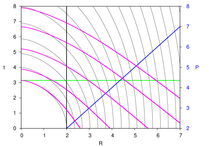
This is the easiest case to interpret, since all the shells have a Newtonian negative energy. The marginally bound shell with and starts off at infinity, while the shell with and starts off at the Schwarzschild radius.
B.1.2
The effective potential is a monotonically increasing function and thus all lines with intersect at some . No particle is unbound, also not those with . This means that the cosmological constant ’always wins’ in attracting radial shells to the center.
If and thus and we find similar solutions as (B.9):
| (B.10) |
with as calculated in appendix A. These shells start at rest at at some radius with : the upper limit follows from and thus .
For all other start radii the relations , and hold, together with the solution
| (B.11) |
In both cases, the shell that starts at has and hence shell parameter . The shell that is marginally bound, starting off at has and .
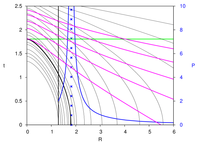
B.1.3
In this case, the effective potential has a maximum at , where it attains the value . We need in order to have a metric with the required signature. Hence . If (case that is not relevant in the context of this paper), there is universal expansion. The presence of the black hole makes bound shells possible in a finite part of space. Space is confined to the inner radius and the outer radius , with and as defined in appendix A.
Radial shells that have zero radial velocity at some R between and have therefore , hence, with (B.7), and .
Because has a maximum at , points at rest at at some radius will fall into the black hole according to (B.10). On the contrary, points at rest at at some radius will be driven towards , and beyond toward infinity. The shell has the same role as the Schwarzschild radius, but instead of a black hole horizon it is a ’black sky’ horizon. In this latter case the motion is not defined by (A.1), which uses . Instead, these shells are given by
| (B.12) |
We will not discuss them further.
A point at rest at will remain at rest, on an unstable shell though. For that shell
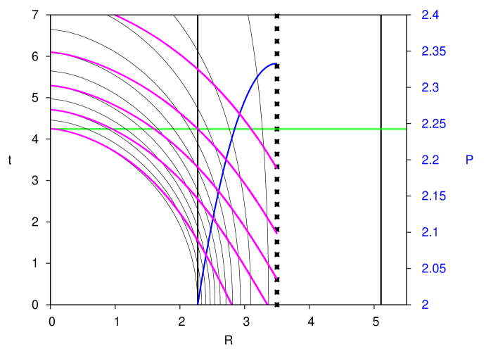
B.2 The Novikov metric
In this subsection we will transform the Schwarzschild- metric into a representation in comoving coordinates. One such a frame can be obtained by considering a swarm of shells of the kind we have just come to consider. The essential feature of the swarm is that they all have zero radial velocity at the same Schwarzschild- coordinate time . We arrange the swarm of shells such that at that time all allowed radii are uniquely occupied. We denote with the proper time on a shell (i.e. the arc length), and since it is a proper time, it can be used as a coordinate time that all shells can agree on. We set at the start of their journey, and thus all shells have zero Schwarzschild- radial velocity at coordinate time and proper time in their shell . At any later coordinate time , any allowed radius will be covered by a shell, however with increasing radial Schwarzschild- velocity as progresses, since coordinate shells crash into the black hole or disappear into the black sky, but are replaced by others with non-zero velocity.
We now consider the coordinates . These coordinates were first introduced by Novikov (see [1]). We call the (Novikov) shell label. We consider only the coordinate shells with label that fall into the black hole. We again must distinguish 3 cases.
For , we see that after a warm-up time that is equal to the free fall (proper) time of shell all radii are covered, as indicated in figure 18. From that time on, the minimum shell label, which was initially , will steadily increase. All shells have
For we define the warm-up time as the time needed to crash the outermost shell of the first family with into (see figure 19). From that time on, all of space is covered by shells with .
For the warm-up time is equal to the crash time of shell (see figure 20), be it that we only consider the region of space that allows infalling shells. All these shells have .
Note that, as has been remarked in the captions of the figures 18, 19 and 20, these warm-up times can be relaxed somewhat by considering the light shells, but this is of no particular importance.
From the above analysis, we conclude that
| (B.13) |
with the convention that .
For the transformation of the Schwarzschild- metric (4.3) into , we make use of (B.2) and (B.7)
| (B.14) |
together with (B.3) and (B.7) which can be written as
| (B.15) |
The first equality in these equations follows from the fact that the ’Novikov swarm’ evolves at constant and hence
| (B.16) |
and similarly for . Note that we do not seek (and need) an explicit expression for .
The metric (4.3) transforms into
| (B.17) |
after some rather lengthy calculations, especially to verify algebraically that the cross term
| (B.18) | |||||
is zero. This must, since the shells start at rest at , therefore they are orthogonal to 3-space at that time and hence, (B.17) is the Gaussian extension into proper time of a 3-metric. In order to prove this, one can consider its time derivative and show that it is zero. We are, of course, free to redefine the origin of time at any time, as long as the shells are such that they once were all together at rest at the same moment.
The metric (B.17) is of the form (2.1). In fact, it is a special case of (2.1), since substitution of by and the choice transforms (2.1) in (B.17). Interestingly, just as is the case for metric (2.1), does not appear explicitly as a number in (B.17), and that information is fully contained in . The metric is valid for if , or if .
B.3 Orbits
Since the Novikov metric has the same form of (2.1), the analysis developed in section 8 is valid, with the additional simplification that there is no singularity in the metric. All radii, also these inside , can be treated equally.
As an example, we will now show that inside only inward motion is possible. Therefore we consider light that is sent radially in or out :
| (B.19) |
The increment in equals
| (B.20) |
which reads, taking into account (B.15)
| (B.21) |
Clearly, if , i.e. inside , the right hand side is always negative.
In the following figures, the structure of the orbits is elucidated by showing the light cones at various ’places’ in the Novikov representation.
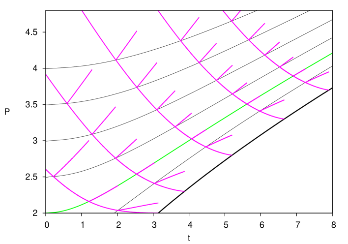
B.4 Transition from orbit representation between Schwarzschild- and Novikov coordinates
In the Schwarzschild- frame a stationary observer will assign to an infalling Novikov-shell the local Lorentzian radial velocity
| (B.22) |
The numerator in the first fraction stands for a length measurement, the denominator for a time measurement. In a Novikov frame (note that there are an infinite number of them, since one can choose ), on the other hand, a stationary observer will find the Schwarzschild- shells of constant moving radially outward. The Novikov observer’s local Lorentzian radial length measurement equals
| (B.23) |
which happens at constant . Hence we can rewrite as
| (B.24) |
and the Novikov stationary observer assigns to the outgoing Schwarzschild- shell the local Lorentzian radial velocity
| (B.25) | |||||
Both velocities are equal in absolute value, as also follows from (B.14). Note that, using (B.3) and (B.7),
| (B.26) |
in the region of space where the Schwarzschild- metric is valid ().
An orbit in the Schwarzschild- metric transforms into an orbit in the Novikov metric as follows. As above, we assign to both the stationary Schwarzschild- observer and the stationary Novikov observer their own local Lorentzian coordinate frame with the -axis in the outward direction and the axis in a tangential direction. In the local Lorentzian Schwarzschild- frame, a particle with coordinates and coordinate velocity has a velocity
| (B.27) |
This velocity transforms in a velocity in the local Lorentzian Novikov frame with the Lorentz transformation
| (B.28) |
Hence, the coordinate velocities in the Novikov frame are
| (B.29) |
and the coordinates are with depending on the particular Novikov frame (using the black lines in figures 21, 22 or 23).
The Lorentz transformation causes a kind of refraction. Denoting
| (B.30) |
and the respective angles with the outward radial direction by and , we can calculate these angles with
| (B.31) |
For light, the above relations simplify to the well-known
| (B.32) |
Wavelength is transformed with
| (B.33) |
The inverse refraction transformations are, of course, obtained by simply replacing with and interchanging and .
Appendix C A transport theorem for coordinate intervals
We consider 2 particles (material particles or photons) that are launched on the same orbit but separated by a coordinate interval . We set out to study how is transported along a geodesic, where, for a material particle, is the arc length along the geodesic or, for a photon, is a parameter such that the familiar geodesic equations hold:
| (C.1) |
with and dummy indices. The evolution of the coordinate along the 2 orbits therefore can be denoted by and . If we denote
| (C.2) |
for the first particle, then
| (C.3) |
for the second particle. Hence the transport differential equation
| (C.4) |
We consider a metric for which is independent of and , . Hence, from the we get
| (C.5) |
with for a material particle and for light, and thus, upon partial differentiation with respect to ,
| (C.6) |
If we compare this expression with the -geodesic we find
| (C.7) |
and thus, with (C.4)
| (C.8) |
Hence the product
| (C.9) |
is a constant along any orbit.
For the 3 metrics we consider in this paper it suffices to consider orbits in the meridional plane for which is a constant. We find that is a constant. Since the -geodesic yields in addition that is a constant (third equation of the system (8.1)), we find the obvious constant , indicating that there is rotational symmetry.
Somewhat less obvious is the application of this theorem to the coordinate in the Schwarzschild- metric, for which the same argument as above yields that is a constant along a geodesic. From an analogous equation as (10.1) we find that is a constant of the motion, and hence also . It expresses the fact that orbits calculated at different times but with the same initial conditions are identical, except for the time translation. This is instrumental in the derivation of the formula for the gravitational redshift.
For the L-T metric we obtain, with (8.7),
| (C.10) |
as a constant along any geodesic, but here is not a constant.
Appendix D The angular distance
D.1 Definitions
The angular distance at the observer is defined as the ratio of the linear size of an infinitesimal light emitting rod over the angle it subtends at the observer:
| (D.1) |
with the rod placed in the plane of the light ray that connects emitter and observer. It is at all times perpendicular to the tangent of the light ray. Therefore, is a length measurement at the emitter at the time of emission , while is an angle measurement at the observer at the time of observation . Because isotropy is lost in the spherical case, will depend on the viewing direction.
Similarly, we will need to consider the angular distance at the emitter
| (D.2) |
which is the ratio of the linear size of a similar rod at the observer over the angle it subtends at the emitter. We will now derive expressions for these ratios.
We placed the rod in the plane of the light ray, but it need not be so. If we simplify the situation in a non-essential way by replacing the light ray by a line in Euclidean space, the rod could be on any plane through that line. So we can also state that the rod fills a circle with surface , subtended by a solid angle
| (D.3) |
A finite circle at the emitter need not be seen as a circle by the observer. In the limits and which we consider here, this will be the case, though. We can therefore easily pass from length and angle to surface and solid angle by squaring the ratios (D.1) and (D.2). Hence it also suffices to consider and in the plane of the light ray.
We need to calculate the infinitesimal divergence which is at every point along the orbit perpendicular to the tangent, and which is the consequence of a small deviation from the initial direction . If the integration along the orbit is executed backwards (starting from the observer, with initial condition ), we obtain , which is the angular distance at observer (D.1). If executed forward (starting from the emitter, with initial condition ) we obtain .
D.2 The equations
In the following analysis, we do not need to make the above distinction and we will consider the generic . The problem at hand is known as the equations for the geodetic deviation. It can be shown quite generally that these are second order differential equation involving covariant differentiation and the Riemann tensor. We will follow a more intuitive (be it more elementary) approach.
Along the orbit, a small deviation from will generate
| (D.4) |
From the expression of in (8.3), we obtain
| (D.5) |
where we introduced the shorthand notation
| (D.6) |
The second equation of (8.3) yields
| (D.7) | |||||
Finally, the second equation of (8.17) yields
| (D.8) | |||||
As for the initial conditions, we denote
| (D.9) |
which are the components of a vector that is proportional to the local Lorentzian velocity vector (it is identical at the start of the light ray, when ). We can assume . Initially, the light ray makes an angle with the outgoing normal, given by . A small deviation leads to . These components are not independent because . We obtain
| (D.10) |
and
| (D.11) |
From this equation and the linear structure of equations (D.5), (D.7) and (D.8) we see that we can divide all the infinitesimals by in order to obtain equations involving finite quantities.
It is possible to combine all the above equations using the expression (D.4). The orthogonality of with implies
| (D.12) |
using geometric considerations and . We obtain, after some calculations:
| (D.13) | |||||
Similarly, we can transform equation (D.8):
| (D.14) | |||||
The differential equations (D.13) and (D.14) are sufficient to calculate , and can be added to the equations of the light ray. As to the initial conditions, we start with . The orthogonality condition yields .
D.3 A theorem
A further simplification, based on , and thus , can eliminate altogether. Therefore we write
| (D.15) | |||||
which transforms (D.13) into
| (D.16) | |||||
This equation could at first sight replace one of the equations (D.8) and (D.13), were it not that it needs the resolution of a at the turning points of the light ray (), which implies a further derivative. Therefore the above equation is only useful as a further relation involving .
We now apply/verify equation (D.16) in 3 cases. Firstly, for small , we obtain
| (D.17) |
which is the Euclidean limit.
Secondly, in the Euclidean case , we have exactly, and (D.16) simplifies to
| (D.18) |
which is a rather obvious trigonometric relation valid for a straight line. This example also shows that (D.16) is not sufficient to calculate , since information on the orbit must also be included, in this case the fact that the orbit is a straight line.
Thirdly, we can also verify equation (D.16) in the synchronous case. From the Euclidean case, we know that hidden in (D.16) is a geometrical relation of the orbit. We adopt the notations of section 9.5. From geometrical considerations we now that
| (D.19) |
where we made use of (6.8) and (6.3). Geometry learns us also that we can simplify the orbit to a radial one starting from the origin, and thus and . Equation (D.16) then reduces to
| (D.20) |
yielding
With the aid of (9.48), this expression can be seen to yield an identity. This special case is also an occasion to see the sheet parameter ‘at work’, since in the left hand side we find , while in the right hand side we find .
Appendix E The surface brightness and flux
E.1 The surface brightness
An elementary surface at the emitter sends photons to an elementary surface of the observer. Therefore the emitter sends his photons within his elementary solid angle and the observer receives them within her elementary solid angle . The light paths that materialize this relation are not straight lines, nor can they be taken to be the simple radial geodesics as in the synchronous case, but have to be calculated. Conservation of photons requires
| (E.1) | |||||
with (resp. ) the number of photons emitted (resp. observed) at time , location r, with wavelength and direction , during a time interval , on an elementary surface , within an elementary solid angle and in a wavelength range . Defining the surface brightness as
| (E.2) |
at a specific wavelength and per unit of time, we obtain
| (E.3) |
where we used
| (E.4) |
We of course recover the local Lorentzian invariant , but spacetime contributes a factor due to the effect that the infinitesimal lightcone with top at the emitter is not equal to the one with top at the observer.
E.2 The flux
As for the fluxes, we start from (E.3). We integrate the left hand side at the observer over the total solid angle subtended by the emitter, and we integrate the right hand side over the full visible surface of the emitter, thereby capturing all photons. Hence,
| (E.9) |
The integration on the right hand side equals, for an isotropic emitter, the luminosity at (which is a power) divided by , while the integration on the left hand side equals the flux (which is power per unit surface) observed at . Hence
| (E.10) |
The observed flux in band , that is the redshift transformed band from the band at the emitter, equals
| (E.11) |
Turning to magnitudes, we recall that an absolute magnitude is a flux at 10 pc. Hence, we rewrite (E.11) as
| (E.12) |
in which we recognize inside the big brackets the flux of the emitter if it were placed at . Passing to magnitudes, we obtain
| (E.13) |
In our unit of length
| (E.14) | |||||
E.3 The luminosity distance
Appendix F Distribution functions
In the presence of a static spherical mass distribution centered at , geodetic motion has the constant of the motion (10.1):
| (F.1) |
In this expression denotes the mass of the particle. At the distance an observer measures time with a ’shell time’ , and the metric yields
| (F.2) |
Hence
| (F.3) |
with
| (F.4) |
the relativistic energy as measured by the shell observer at , and momentum and velocity observed by the same observer.
Because of the spherical symmetry, the angular momentum is also conserved. Denoting by the radial component and by the absolute value of the component perpendicular to the radial component (and hence ), we have . Any isotropic distribution far from the mass distribution therefore transforms to
| (F.5) |
at distance . In this equation the already accounts for the integration over the position angle of the momentum vectors perpendicular to the radial component, since the distribution does not depend on it. For small velocities and a weak field, we of course recover
| (F.6) |
expressing the fact that at infinity, a particle has climbed the potential well.
When all that keep the radicand positive are allowed, it is not too hard to work out the expression of all the velocity moments
The Boltzmann distribution
| (F.9) |
can be integrated with (F). We obtain the density
which yields
| (F.11) |
with the Bessel function of the third kind in the imaginary argument.
If the argument of is small, as is likely the case in a compact phase, then the approximation is valid. If it is large, as is likely the case in the current epoch, we have . Hence
| (F.14) |
Another normalisation of (F.11) is
| (F.16) |
with the density of the isothermal distribution in the absence of a mass distribution. It is computationally convenient to consider the function
| (F.17) |
yielding
| (F.18) |
If the quantity is small, which is the case even for very massive and very compact mass concentrations on distances larger than a parsec, we can further simplify to
| (F.19) |
If is large, then
| (F.20) |
For the isotropic pressure , defined as one third of the moment of order 1 in the expression (F), we obtain
| (F.21) |
In the presence of a mass concentration, these distributions apply to the ensemble of all particles, whether they are bound to the structure or not. If we restrict us to the bound particles, the same analysis would apply but the integration would extend to rather than . Here we will consider only the analogue of (F.20), which is the well-known expression
| (F.22) |
with
| (F.23) |
the normalized incomplete gamma function.
Appendix G Definition of symbols
| Symbol | Equation | section | Name |
|---|---|---|---|
| 3.4.2 | center of the universe | ||
| E.15 | luminosity distance | ||
| , | D.1, D.2 | angular distance at observer, emitter | |
| , | F.4 | rel. en. meas. by stat. obs., rest mass en. | |
| , | 10.1, B.2, F.1 | (norm.) rel. en. measured at infinity | |
| 8.3 | 9.1 | norm. rel. en. measured by comoving obs. | |
| 11.39, 11.43 | norm. rel. en. measured by a stat. obs. at | ||
| 11.3.2, 11.56 | min. of non-plunging orbit around a BH | ||
| 11.52 | min. of non-plunging orbit around a BH | ||
| 11.100 | normalisation in Fermi-Dirac distr. | ||
| , | E.10, E.11 | obs. flux: at specific wavelength, in band | |
| gravitational constant | |||
| , | 3.33, 3.34 | tangential Hubble parameter | |
| 3.35 | |||
| 2.9 | observed value for | ||
| 9.27 | tangential deceleration parameter | ||
| 9.28 | mixed deceleration parameter | ||
| 9.10 | radial Hubble parameter | ||
| 9.27 | radial deceleration parameter | ||
| 9.28 | mixed radial deceleration parameter | ||
| , | E.2, E.3 | surface brightness at emitter, observer | |
| , | E.2 | rad. power at spec. wavelength, in band | |
| 2.20, 4.3, 6.26 | total eff. gravit. mass with dim. of length | ||
| 11.128 | total mass in an exponential envelope | ||
| 10.2 | |||
| 11.1 | in units of | ||
| 11.128 | total mass in a Hernquist bulge | ||
| 11.1 | geom. mass of BH hole in units | ||
| E.14 | absolute magnitude of emitter in band | ||
| 11.4.1 | total mass of a (spiral) galaxy | ||
| 2.12 | cumulative mass inside shell | ||
| 11.7 | cumulative mass inside radius | ||
| 5.1 | mass of shell | ||
| 2.22, 6.16 | total mass of the universe | ||
| 10.2 | mass of black hole | ||
| 3.4.2 | position of the observer | ||
| 4.1, B.5 | max. shell param., Novikov shell label | ||
| , | 11.10, 11.58 | (dimensionless) radial pressure | |
| , | 11.2 | (dimensionless) tang. pressure | |
| , | 11.2 | tangential pressures | |
| F.21 | (neutrino) pressure |
| Symbol | Equation | Section | Name |
|---|---|---|---|
| 3.3 | 2.1 | radius | |
| , | 3.26, 3.27 | 4D, 3D Riemann curvature scalar | |
| 3.13 | maximum radius of shell | ||
| 5.1 | radius of thin shell | ||
| 4.2 | max. radius of a dust ball / universe @ | ||
| 4.9 | maximum radius of the universe | ||
| B.1 | Schw- radius of a Novikov shell | ||
| , | 11.128 | scale length of exp., Hernquist bulge | |
| 4.11 | Schwarzschild radius | ||
| 4, B.1 | black sky radius | ||
| 6.3 | coefficients of behaviour of @ | ||
| , | 10.5 | 11.3 | norm. radius around a black hole, specific |
| 11.20 | outer boundary of mass distr. around BH | ||
| 11.65, 11.66 | inner boundary of mass distr. around BH | ||
| 10, 11.3 | of circ. orbit with smallest and | ||
| , | 10.8 | extrema in the eff. potential around BH | |
| 6.3 | radius of a synchronous universe | ||
| , | 9.5 | @ epoch of emission, observation | |
| , | E.1 | elementary surface at emitter, observer | |
| , , | 2.25, 2.26 | 5.1 | tangential stretch rate, inside shell |
| 11.97 | absolute temperature, in units of 2 K | ||
| 11.3.9 | 2 Kelvin | ||
| 11.3, 11.10 | energy-momentum tensor | ||
| 2.11 | elementary volume element | ||
| 10.5, 11.33 | effective potential of an orbit with given | ||
| 4.4, B.3 | effective potential of a radial orbit | ||
| 10.9 | max. closest to the black hole | ||
| 11.4.1 | circular velocity of a flat rotation curve | ||
| , | 4.7, B.28, B.30 | Lorentzian velocities in Novikov frame | |
| , | 4.8, B.27, B.30 | Lorentzian velocities in Schw- frame | |
| 2.3 | radial scale factor | ||
| 6.37 | coefficients of behaviour of at | ||
| 6.44 | coef. of the singularity of at | ||
| 2.1 | cartesian coordinate | ||
| 2.1 | cartesian coordinate | ||
| 3.31, 3.32 | embed. surf. isom. repres. 2D universe | ||
| 2.1 | cartesian coordinate |
| Symbol | Equation | Section | Name |
|---|---|---|---|
| , | 11.97 | parameter in isoth. distr., in units of | |
| 11.98 | |||
| 11.99 | for 1 eV and 2 K | ||
| 5.6 | for shell | ||
| B.5 | in function cyc for a Novikov shell | ||
| B.8 | of Novikov shell that starts at | ||
| 3.6 | |||
| 3.39 | |||
| c, | velocity of light | ||
| 3.3 | solution of the evolution equation | ||
| A.1 | cyc as function of parameters and state | ||
| 3.41, 3.42, 3.50, 3.51 | cyc for | ||
| 2.3, 6.23 | energy function | ||
| 3.25, 6.23 | central scaling of | ||
| 5.3 | binding energy of shell | ||
| 6.5 | for synchronous universe | ||
| 11.100 | degr. of freedom in Fermi-Dirac distr. | ||
| C | metric tensor | ||
| h | 11.100 | Planck’s constant | |
| 8.1, 10.3 | specific relativistic angular momentum | ||
| 10.6, 11.33 | normalized | ||
| 11.69 | min. of marg. bnd non-plung. orbit | ||
| 10, 11.3 | smallest for non-plunging orbits | ||
| 11.52 | of a marginally non-plunging orbit | ||
| 11.47 | min. of non-plung. orbit given | ||
| 9.1 | geometrical distance | ||
| , | D.4 | elem. dist. perp. to a light ray | |
| , | D.1 | at observer, emitter | |
| 2.6, 2.13, 2.23, 6.26 | eff. grav. mass function | ||
| 11.4 | eff. gravit. mass function around BH | ||
| 3.10, 6.26 | normalized | ||
| 11.4, 11.6 | normalized | ||
| 9.3, 9.5, E.2 | magnitude-redshift relation | ||
| 10.1 | 8.1, F | rest mass | |
| 3.21, 6.26 | central scaling of | ||
| 6.10 | for synchronous model | ||
| 5.1 | gravitating mass @ shell i | ||
| 5.2 | |||
| 11.97 | neutrino mass in units of 1 eV | ||
| 11.3.9 | mass equivalent of 1 eV | ||
| E.14 | observed magnitude in band | ||
| 9.1, C, F | param. of light path, momentum | ||
| 3.4 | shell parameter of shell with label | ||
| 3.11 | normalized shell parameter |
| Symbol | Equation | Section | Name |
|---|---|---|---|
| 3.18 | scaling for | ||
| 6.18 | for synchronous universe | ||
| 5.6 | for shell | ||
| , | 11.40 | F | (norm.) tang. comp. of linear momentum |
| , | 11.43 | F | (norm.) rad. comp. of linear momentum |
| 11.3.2, 11.47 | min. for a non-plunging orbit around a BH | ||
| 11.54 | tang. comp. of of unstable pericenter orbit | ||
| 3.37 | classical deceleration parameter | ||
| 2.1 | shell label | ||
| 2.19 | normalized shell label | ||
| a specific shell label | |||
| 6.24 | label of shell inside which | ||
| 6.25 | label of isolated shell on which | ||
| , | E.1 | position vector of observer, emitter | |
| 6.26 | inside which has a synch. behaviour | ||
| 2.16 | of comoving matter outer boundary | ||
| 6.23 | inside which has a synch. behaviour | ||
| 6.28 | inside which the universe is synchronous | ||
| , | 6.27 | at the interior/exterior of which is const. | |
| 2.1, 8 | arc length | ||
| , t | 2.5 | (c ) cosmic time | |
| 4.2.2 | c cosmic time in relation with the Schw- metric | ||
| a specific cosmic time | |||
| 3.45 | at which a given is realized @ shell | ||
| 3.14 | cosmic time of max. expansion of shell , if bound | ||
| , | 9.1 | cosmic time of emission, observation | |
| 2.18 | validity time limit of the metric | ||
| 11.4.1 | cosmic time oat which neutrino’s bind to a galaxy | ||
| , | 4.3, 4.5 | (c ) Schwarzschild- coordinate time | |
| B.2 | Schwarzschild- time of a Novikov shell | ||
| 11.3 | time of stationary observer at in a Schw- metric | ||
| 6.29 | |||
| F | velocity measured by stationary observer | ||
| B.22, B.25 | rad. vel. diff. between Schw- and Novikov frame | ||
| 4.15 | Lorentzian rad. vel. in the inner Schw- metric | ||
| 11.3.9 | unit of velocity | ||
| 11.38 | tang. component of measured by stat. observer | ||
| 11.4.1 | velocity vector with respect to comoving observer | ||
| 8.14 | coef. in the regularized rad. equ. of an orbit | ||
| , | 8.16, 8.2, 8.13 | Lorentzian radial velocities | |
| 3.13 | A | smallest real root for cyc of | |
| , | A | the 2 roots of that are not | |
| , , | 9.1 | redshift, as function of orbit parameter, Hubble law | |
| 3.57 | standard cosmological redshift |
| Symbol | Equation | Section | Name |
|---|---|---|---|
| cosmological constant | |||
| 11.11 | |||
| 11.11 | normalised | ||
| 11.66 | |||
| 6.27 | |||
| 11.18, F.2 | gen. relat. analog of Newt. binding potential | ||
| 11.13, 11.127 | normalized | ||
| 2.2 | elementary solid angle | ||
| , , | 3.54 | standard cosmological ’s | |
| , | E.1 | elementary solid angle at emitter, observer | |
| 6.30 | shorthand for | ||
| 6.23 | coefficients of the expansion of at | ||
| 6.31 | shorthand for | ||
| 6.26 | coefficients of the expansion of at | ||
| 11.57 | mean of a mass distribution around a black hole | ||
| 6.33 | shorthand for | ||
| 6.27 | coefficients of the expansion of at | ||
| F.2 | |||
| 8.10 | |||
| 6.41 | exponent in the asymptotic behaviour of at | ||
| 3.7 | sign of in representation (a) | ||
| B.7, B.13 | for Novikov metric, sign of | ||
| 3.8 | shorthand for in representation (b) | ||
| 8.12 | sign constant indicating the sheet of the universe | ||
| 8.5 | 1 for a massive particle and 0 for a photon | ||
| 2.1 | polar coordinate | ||
| 9.7 | angle of velocity with respect to the radial direction | ||
| , | B.31 | in Schwarzschild- frame, in Novikov frame | |
| , | D.1 | elementary angle at observer, emitter | |
| 2.6, 2.10 | |||
| 6.23 | exponent in the asymptotic behaviour of at | ||
| , | B.33 | wavelength in Schwarzschild- frame, in Novikov frame | |
| , | E.1 | wavelength at observer, at emitter | |
| 11.2 | log of coef. of in a static spherical diagonal metric | ||
| 6.26 | exponent in the asymptotic behaviour of at | ||
| 6.27 | exponent in the asymptotic behaviour of at | ||
| 11.2 | log coef. of in a static spherical diagonal metric | ||
| 8.9 | regularized shell label |
| Symbol | Equation | Section | Name |
|---|---|---|---|
| 2.6 | local Lorentzian mass (dust) density of the universe | ||
| 3.20 | scaling for | ||
| 6.19 | for the synchronous universe | ||
| 2.8 | critical mass density | ||
| 11.4.2 | mass density of a Milky Way type galaxy, excluding DM | ||
| 11.117 | mass density of an isothermal sphere | ||
| , | 11.2 | Fermi-Dirac particle density around a BH, normalized | |
| 11.124 | neutrino mass density of the universe on galactic scales | ||
| 5.1 | surface density of thin shell | ||
| 10.3 | proper time | ||
| 2.1 | longitudinal coordinate | ||
| 3.1, 6.27 | shell phase function | ||
| 6.27 | |||
| 6.7, 6.48 | shell label that regularizes | ||
| 3.2 | state of shell @ | ||
| 5.6 | for shell | ||
| , | 3.1, A.1 | integral that defines cyc implicitly | |
| B.5 | zero radial velocity state of a Novikov shell | ||
| 3.13, A.2 | state of shell @ max. expansion | ||
| 3.5 | shell frequency | ||
| 3.12 | normalized shell frequency | ||
| 3.22 | central shell expansion freq. | ||
| 5.6 | for shell | ||
| 6.21 | in synchronous universe |