Uniformly-moving non-singular dislocations with elliptical core shape in anisotropic media

Abstract

To allow for “relativistic”-like core effects, an anisotropic regularization of steadily-moving straight dislocations of arbitrary orientation is introduced, with two scale parameters $a_{\parallel}$ and $a_{\perp}$ along the direction of motion and transverse to it, respectively. The dislocation core shape is an ellipse. When $a_{\perp}/a_{\parallel}\to 0$, the model reduces to the Peierls-Eshelby dislocation, the fields of which are non-differentiable on the slip plane. For finite $a_{\parallel}$ and $a_{\perp}$, fields are everywhere differentiable. Applying the author’s so-called “causal” Stroh formalism to the model, explicit expressions for the regularized fields in anisotropic elasticity are derived for any velocity. For faster-than-wave velocities, Mach-cone angles are found insensitive to the ratio $a_{\parallel}/a_{\perp}$, as must be. However, the larger $a_{\parallel}$, the weaker the intensity of the cone branches. An expression is given for the radiative dissipative force opposed to motion. From this expression, it is inferred that the concept of a “radiation-free” intersonic velocity can, when not applicable, be replaced by that of a “least-radiation” velocity.

I Introduction

This work is concerned with the regularization of dislocation fields, for a straight dislocation moving steadily in an anisotropic medium (Sáenz, 1953; Bullough and Bilby, 1954; Teutonico, 1962). Indeed, the so-called standard model of dislocations (Anderson et al., 2017), based on zero-width Volterra dislocations, produces singular fields at the origin. Various models have been proposed to tame this singularity. The oldest one is perhaps the Peierls-Nabarro model of a static dislocation (Peierls, 1940; Nabarro, 1947; Schoeck, 2005), which was extended to steady motion (Eshelby, 1949, 1953; Weertman, 1969a, b; Weertman and Weertman, 1980; Markenscoff and Ni, 2001b; Rosakis, 2001; Pellegrini, 2014). However, as pointed out by Eshelby (Eshelby, 1949), such Somigliana dislocations generate non-differentiable fields on the slip plane.

Since, a variety of regularization techniques were used to make the fields partially or fully nonsingular, mostly in a static context. Early models have been reviewed by Cai et al. (2006), who put forward a phenomenological model of a dislocation with isotropic core of finite size, applying it to static dislocation segments. Another isotropic-core model has been proposed by Pellegrini and Lazar (2015) to compute the elastodynamic fields of arbitrarily-moving dislocations in an isotropic medium (Lazar and Pellegrini, 2016). Also, non-locality is an efficient regularizing device. In this line of thought, non-local models have been introduced in the framework of gradient elasticity, such as a 6-parameter anisotropic core model, from which non-singular static fields in anisotropic crystals have been derived (Lazar and Po, 2015a, b; Po et al., 2018).

The present work describes an extension of the Pellegrini-Lazar model to elliptical cores, with application to steady motion in an anisotropic medium. The aim is to devise a simple model with two different regularizing length scales —one in the transverse direction, and the other one in the direction of motion— so as to allow for ‘relativistic’ core-width variations in the latter direction (Eshelby, 1949). Such variations, which can be considered as the elastic counterpart of a Lorentz-Fitzgerald contraction, are important for motions of velocity comparable to wavespeeds in the crystal, including faster-than-wave velocities (Bullough and Bilby, 1954; Eshelby, 1956; Weertman, 1967, 1969b; Rosakis, 2001; Lazar, 2009; Pellegrini, 2012, 2014); see, e.g., Auld (1973) for waves in crystals. However, the two length scales are considered as fixed parameters hereafter, this work being focused on obtaining explicit field expressions.

The paper is organized as follows. Section II introduces the elliptical-core model, and shows that it can be considered a fully-regularized anisotropic extension of the Peierls-Eshelby model of a dislocation (Peierls, 1940; Nabarro, 1947; Eshelby, 1949). Differences with the Lazar-Po approach (Lazar and Po, 2015a, b) are pointed out. The elastic fields of the moving dislocation are derived in Section III. The method used relies on the Stroh formalism for dislocations moving through an anisotropic medium (Stroh, 1962; Anderson et al., 2017; Chadwick and Smith, 1977; Bacon et al., 1979; Lothe, 1992; Wu, 2000; Barnett and Zimmerman, 2002; Blaschke and Szajewski, 2018). This formalism was modified in a causal way in Pellegrini (2017) to provide a general framework for field computations at any velocity, including faster-than-wave ones. From these results the dissipative force acting on the dislocation is obtained. Section IV is devoted to the isotropic limit of the model. Numerical results are presented in Section V. Section VI concludes the article. An Appendix gathers the most technical calculations.

Our conventions for the Fourier transform of a space- and time-dependent function $f(\mathbf{r},t)$ are

$$f(\mathbf{k},\omega)=\int\mathrm{d}^{d}\!x\,\mathrm{d}t\,f(\mathbf{r},t)\mathrm{e}^{-\mathrm{i}(\mathbf{k}\cdot\mathbf{r}-\omega t)},\,f(\mathbf{r},t)=\int\frac{\mathrm{d}^{d}\!k}{(2\pi)^{d}}\frac{\mathrm{d}\omega}{2\pi}\,f(\mathbf{k},\omega)\mathrm{e}^{\mathrm{i}(\mathbf{k}\cdot\mathbf{r}-\omega t)},$$ (1)

where integrations with respect to the space variable $\mathbf{r}$ and the wave vector $\mathbf{k}$ are over the $d$-dimensional space ($d=2$), and integrations with respect to the time $t$ and the angular frequency $\omega$ are over $\mathbb{R}$. Bold and sans-serif typefaces are used, respectively, to denote vectors ($\mathbf{a}$) and dyadic tensors ($\mathsf{A}$) of components $A_{ij}$. A hat denotes a unit vector whenever it is built from an existing non-unit vector, e.g., $\mathbf{\widehat{k}}\equiv\mathbf{k}/k$. This ‘hat’ notation is not used for vectors specifically introduced as unit vectors. Finally, matrix or vector scalar products are denoted by a dot, which represents a contraction with respect to the tensor index in between when no confusion is possible: $\mathsf{a}\cdot\mathsf{b}$ is the matrix of components $a_{ik}b_{kj}$.

II Regularization: a nested family of dislocation models

This section introduces a nested family of dislocation models rooted in the Peierls model. The dislocation is represented by the plastic eigenstrain tensor $\beta^{\rm p}_{ij}(\mathbf{r},t)$ (Mura, 1987). The dislocation, moving at constant velocity $\mathbf{v}$, is such that in the direct and Fourier representations (respectively),

$$\beta_{ij}^{\rm p}(\mathbf{r},t) =\beta_{ij}^{\rm p}(\mathbf{r}-\mathbf{v}t),\qquad\beta_{ij}^{\rm p}(\mathbf{k},\omega)=(2\pi)\delta(\omega-\mathbf{v}\cdot\mathbf{k})\beta_{ij}^{\rm p}(\mathbf{k}).$$ (2)

Its shape is assumed rigid (i.e., time-independent), and completely characterized by $\beta_{ij}^{\rm p}(\mathbf{r})$, or by $\beta_{ij}^{\rm p}(\mathbf{k})$ in the Fourier representation. For steady-state motion, all quantities in direct space depend only on the position vector $\mathbf{r}-\mathbf{v}t$ with respect to the dislocation position $\mathbf{v}t$, where $\mathbf{v}$ is the velocity. Hereafter, this vector is simply denoted by $\mathbf{r}$ for conciseness, all calculations being done in the co-moving frame. We introduce orthogonal unit vectors $\mathbf{m}$ and the slip plane normal $\mathbf{n}$ along the $x$ and $y$ coordinate axes, respectively. Motion is along $\mathbf{m}$ so that $\mathbf{v}=v\,\mathbf{m}$, where $v$ is the signed scalar velocity. The dislocation line is orthogonal to both $\mathbf{m}$ and $\mathbf{n}$.

With $\mathbf{b}$ the Burgers vector, the plastic eigenstrain reads $\beta^{\rm p}_{ij}(\mathbf{r})=n_{i}\widehat{b}_{j}\eta(\mathbf{r})$, where $\eta(\mathbf{r})=\eta(x,y)$ is the slip function along $x$. As it is localized on the slip plane, $\eta(\mathbf{r})$ is a peaked function of $y$ near to $y=0$. It can be written as the convolution of a dislocation-density component $\rho(\mathbf{r})=-\partial_{x}\eta(\mathbf{r})$ by the unit-step Heaviside function $\theta$, as

$$\eta(\mathbf{r}) =\int_{-\infty}^{+\infty}\mathrm{d}x^{\prime}\theta\bigl{(}-(x-x^{\prime})\bigr{)}\rho(x^{\prime},y).$$ (3)

In the Fourier representation, the above expressions become

$$\beta^{\rm p}_{ij}(\mathbf{k}) =n_{i}\widehat{b}_{j}\eta(\mathbf{k}),\qquad\eta(\mathbf{k})=\frac{\mathrm{i}\,\rho(\mathbf{k})}{\mathbf{k}\cdot\mathbf{m}+\mathrm{i}0^{+}}.$$ (4)

Bearing in mind as a reference the singular Volterra model of a point-like dislocation characterized by

$$\rho(\mathbf{r}) =b\delta(x)\delta(y),\quad\rho(\mathbf{k})=b,\quad\eta(\mathbf{r})=b\theta(-x)\delta(y),$$ (5)

the regularized models considered in this work are as follows:

1. Model III: this new model is introduced to represent a dislocation with different half-widths $a_{\parallel}$ and $a_{\perp}$ in both directions.

   With the diagonal matrix $\mathsf{z}=a_{\parallel}\mathbf{m}\otimes\mathbf{m}+a_{\perp}\mathbf{n}\otimes\mathbf{n}$, it reads

   $$\rho(\mathbf{r}) =\frac{b}{2\pi\det\mathsf{z}}\frac{1}{\left[1+\mathbf{r}\cdot\mathsf{z}^{-2}\cdot\mathbf{r}\right]^{3/2}},\quad\rho(\mathbf{k})=b\mathrm{e}^{-\sqrt{\mathbf{k}\cdot\mathsf{z}^{2}\cdot\mathbf{k}}},$$

   $${}\hskip 56.9055pt\eta(\mathbf{r})=\frac{b}{2\pi a_{\perp}}\frac{1-(x/a_{\parallel})/\sqrt{1+\mathbf{r}\cdot\mathsf{z}^{-2}\cdot\mathbf{r}}}{1+(y/a_{\perp})^{2}}.$$ (6)

2. Model II: The Pellegrini-Lazar isotropic-core model (Pellegrini and Lazar, 2015). It is a particular case of (i) for $a_{\parallel}=a_{\perp}=a$, and $\mathsf{z}=a\,\mathsf{I}$.

3. Model I: The semi-regularized Peierls-Eshelby dislocation model (Eshelby, 1953; Rosakis, 2001; Markenscoff and Ni, 2001a, b; Pellegrini, 2010, 2012, 2014, 2017), characterized by

   $$\rho(\mathbf{r}) =\frac{b}{\pi a}\frac{\delta(y)}{1+(x/a)^{2}},\quad\rho(\mathbf{k})=b\mathrm{e}^{-a|k_{x}|},\quad\eta(\mathbf{r})=\frac{b}{\pi}\left(\frac{\pi}{2}-\arctan\frac{x}{a}\right)\delta(y).$$ (7)

   where the length $a$ is the half core width. It is regularized along $x$ but its fields are non differentiable on the slip plane $y=0$.

Models II and III are nonsingular. Relationships between models are obvious from $\rho(\mathbf{k})$. All three models reduce to the Volterra model when $a$, $a_{\parallel}$, and $a_{\perp}\to 0$ simultaneously. Also, the integral over the whole $y$ axis of $\eta(x,y)$ (i.e., the $k_{y}=0$ Fourier mode) gives the same result in Models I, II, and III upon taking $a_{\parallel}=a$. Finally, model III reduces to model I in the limit $a_{\perp}\to 0$ if $a_{\parallel}=a$. All models can thus be considered as members of the same family.

Hereafter, derivations are done for model III, which is no more complicated than model II, except for a few rescalings (in particular, the integrals to be considered are, technically, exactly the same).

The density $\rho(\mathbf{k})$ in (i)₂ is akin to some Fourier dual of that considered by Lazar and Po, who use (in the above notations) the exponential form $\rho(\mathbf{r})\propto\exp{-\sqrt{\mathbf{r}\cdot\mathsf{z}^{-2}\cdot\mathbf{r}}}/$ $[4\pi\det(\mathsf{z})\sqrt{\mathbf{r}\cdot\mathsf{z}^{-2}\cdot\mathbf{r}}]$ as an anisotropic density in the direct space, which is the Green function of the anisotropic Helmholz equation (Lazar and Po, 2015a, b). By contrast, the real-space expression $\rho(\mathbf{r})$ in (i)₁ is finite at $r=0$. Note that, as can be seen from its Fourier transform, it is the solution of the following formal integro-differential equation, which involves the fractional anisotropic Laplacian $(-\bm{\nabla}\cdot\mathsf{z}^{2}\cdot\bm{\nabla})^{1/2}$ (the one-dimensional version of which is the integral operator of the Peierls model (Josien et al., 2018)):

$$\mathrm{e}^{\sqrt{-\bm{\nabla}\cdot\mathsf{z}^{2}\cdot\bm{\nabla}}}\rho(\mathbf{r}) =b\,\delta(\mathbf{r}).$$ (8)

III Elastic distortion, stresses, and forces in Model III

III.1 General setup

The method of computation of the fields in Model III parallels that for Model I in Pellegrini (2017), to which the reader is referred for details. With $\mathbf{u}$ the material displacement vector field, the elastic distortion $\beta_{ij}{:=}\partial_{i}u_{j}-\beta^{\rm p}_{ij}$ is the main field of interest. It is computed by Fourier inversion as

$$\beta_{ij}(\mathbf{r}) =\int\frac{\mathrm{d}^{2}\!k}{(2\pi)^{2}}\left[k_{i}G^{+}_{jp}(\mathbf{k},\mathbf{k}\cdot\mathbf{v})k_{q}c_{pqkl}-\delta_{ik}\delta_{jl}\right]\beta^{\rm P}_{kl}(\mathbf{k})\mathrm{e}^{\mathrm{i}\mathbf{k}\cdot\mathbf{r}}$$

$$=\mathrm{i}\,b_{l}\int\frac{\mathrm{d}^{2}\!k}{(2\pi)^{2}}\left[k_{i}G^{+}_{jp}(\mathbf{k},\mathbf{k}\cdot\mathbf{v})k_{q}c_{pqkl}-\delta_{ik}\delta_{jl}\right]\frac{n_{k}\mathrm{e}^{\mathrm{i}\mathbf{k}\cdot\mathbf{r}}\mathrm{e}^{-\sqrt{\mathbf{k}\cdot\mathsf{z}^{2}\cdot\mathbf{k}}}}{\mathbf{k}\cdot\mathbf{m}+\mathrm{i}0^{+}},$$ (9)

where $G^{+}_{jp}(\mathbf{k},\omega)$ denotes the Fourier expression of the elastodynamic retarded (i.e., causal) Green operator, where Eqs. (2)₂, (4), and (i)₂, have been used, and where the immediate Fourier inversion with respect to $\omega$ has been carried out. The Green operator has the well-known expression

$$\mathsf{G}^{+}(\mathbf{k},\omega)=\lim_{\epsilon\to 0^{+}}[\mathsf{N}(\mathbf{k})-\rho(\omega+\mathrm{i}\epsilon)^{2}\mathsf{I}\,]^{-1},$$ (10)

where $N_{ij}(\mathbf{k}){:=}k_{k}c_{iklj}k_{l}$ is the acoustic tensor built from the elastic tensor $c_{ijkl}$, and $\mathsf{I}$ is the $3\times 3$ identity matrix. The retarded character of $\mathsf{G}^{+}$ stems from the shift of the real angular frequency $\omega$ to complex values with infinitesimal positive imaginary parts, which is a radiation condition (Barton, 1989). The non-trivial limit makes $\mathsf{G}^{+}(\mathbf{k},\omega)$ a generalized function (distribution). The radiation condition in $\mathsf{G}^{+}(\mathbf{k},\mathbf{k}\cdot\mathbf{v})$ can be transferred to $\mathbf{v}$ by introducing the complex velocity vector

$$\mathbf{v}^{\epsilon} =\mathbf{v}+\mathrm{i}\epsilon\,\mathbf{m}=(v+\mathrm{i}\epsilon)\mathbf{m}.$$ (11)

Indeed, upon introducing the dynamic elastic tensor (Sáenz, 1953; Teutonico, 1962), modified with (11) into a complex-valued tensor as

$$\widetilde{c}_{ijkl}^{\epsilon} =c_{ijkl}-\rho v^{\epsilon}_{j}v^{\epsilon}_{k}\delta_{ij},$$ (12)

and the notation $(ab)^{\epsilon}_{il}=a_{j}\widetilde{c}_{ijkl}^{\epsilon}b_{k}$ (Anderson et al., 2017), one has (Pellegrini, 2017)

$$\mathsf{G}^{+}(\mathbf{k},\mathbf{k}\cdot\mathbf{v}) =\lim_{\epsilon\to 0^{+}}\left[\mathop{\mathrm{Re}}+\mathrm{i}\mathop{\text{sign}}(\mathbf{\widehat{k}}\cdot\mathbf{m})\mathop{\mathrm{Im}}\right]\frac{1}{k^{2}}{(\widehat{k}\widehat{k})^{\epsilon}}^{-1},$$ (13)

the real and imaginary parts of which define the reactive and radiative parts of the Green operator, respectively (and, by inheritance, those of the fields that will be computed).

Expression (13) allows for an evaluation of the angular integral over the direction $\mathbf{\widehat{k}}$ in (III.1) by means of the Stroh formalism, while preserving the radiation features of the problem.

III.2 Rescalings

As far as regularization is concerned, the calculation can be made formally isotropic-like in the following manner. Introduce dimensionless position position and wave vectors $\mathbf{r}^{z}\equiv\mathsf{z}^{-1}\cdot\mathbf{r}\equiv(x^{z},y^{z})$, and $\mathbf{q}=\mathsf{z}\cdot\mathbf{k}$. Evidently, $x^{z}=x/a_{\parallel}$ and $y^{z}=y/a_{\perp}$. Letting $G^{+}_{jp}(\ldots)\equiv G^{+}_{jp}(\mathsf{z}^{-1}\cdot\mathbf{q},\mathbf{q}\cdot\mathsf{z}^{-1}\cdot\mathbf{v})$ , this change of variables gives

$$\beta_{ij}(\mathbf{r}) =\frac{\mathrm{i}\,b_{l}}{\det\mathsf{z}}z^{-1}_{ii^{\prime}}\int\frac{\mathrm{d}^{2}\!q}{(2\pi)^{2}}\left[q_{i^{\prime}}G^{+}_{jp}(\ldots)q_{q^{\prime}}z^{-1}_{q^{\prime}q}c_{pqkl}-z_{i^{\prime}k}\delta_{jl}\right]\frac{n_{k}\mathrm{e}^{\mathrm{i}\mathbf{q}\cdot\mathbf{r}^{z}}\mathrm{e}^{-q}}{\mathbf{q}\cdot\mathbf{m}/a_{\parallel}+\mathrm{i}0^{+}}.$$ (14)

Upon introducing the $z$-rescaled elastic tensor

$$c^{z}_{ijkl} =z^{-1}_{jj^{\prime}}c_{ij^{\prime}k^{\prime}l}z^{-1}_{k^{\prime}k},$$ (15)

and noting that $\mathsf{z}\cdot\mathbf{n}=a_{\perp}\mathbf{n}$ and $\det\mathsf{z}=a_{\parallel}a_{\perp}$, expression (14) becomes

$$\beta_{ij}(\mathbf{r}) =\mathrm{i}\,b_{l}z^{-1}_{ii^{\prime}}\int\frac{\mathrm{d}^{2}\!q}{(2\pi)^{2}}\left[q_{i^{\prime}}G^{+}_{jp}(\ldots)(q_{q}c^{z}_{pqkl}n_{k})-n_{i^{\prime}}\delta_{jl}\right]\frac{\mathrm{e}^{\mathrm{i}\mathbf{q}\cdot\mathbf{r}^{z}}\mathrm{e}^{-q}}{\mathbf{q}\cdot\mathbf{m}+\mathrm{i}0^{+}}.$$ (16)

Introduce now the notation $(ab)^{\epsilon z}$ —the $z$-rescaled version of $(ab)^{\epsilon}$— to denote the $3\times 3$ matrix of components $(ab)^{\epsilon z}_{il}=a_{j}z^{-1}_{jj^{\prime}}\widetilde{c}^{\epsilon}_{ij^{\prime}k^{\prime}l}z^{-1}_{k^{\prime}k}b_{k}$. From (13) one deduces

$$\mathsf{G}^{+}(\mathsf{z}^{-1}\cdot\mathbf{q},\mathbf{q}\cdot\mathsf{z}^{-1}\cdot\mathbf{v}) =\lim_{\epsilon\to 0^{+}}\left[\mathop{\mathrm{Re}}+\mathrm{i}\mathop{\text{sign}}(\mathbf{\widehat{q}}\cdot\mathbf{m})\mathop{\mathrm{Im}}\right]\frac{1}{q^{2}}{(\widehat{q}\widehat{q})^{\epsilon z}}^{-1}.$$ (17)

The term within square brackets in (16) does not depend on the modulus $q$, so that the integral over $q$ is done right away using

$$\int_{0}^{\infty}\frac{\mathrm{d}q\,q\,\mathrm{e}^{\mathrm{i}\mathbf{q}\cdot\mathbf{r}^{z}}\mathrm{e}^{-q}}{\mathbf{q}\cdot\mathbf{m}+\mathrm{i}0^{+}}=\frac{\mathrm{i}}{(\mathbf{\widehat{q}}\cdot\mathbf{m}+\mathrm{i}0^{+})(\mathbf{\widehat{q}}\cdot\mathbf{r}^{z}+\mathrm{i})}.$$ (18)

The remaining angular integral over $\mathbf{\widehat{q}}$ in (16) is dealt with by introducing the angle $\phi$ such that $\mathbf{\widehat{q}}(\phi)=-\sin\phi\,\mathbf{m}+\cos\phi\,\mathbf{n}$. By periodicity, the integral is equivalent to one over $\phi$. Introduce the shorthand notation $\left\langle f\right\rangle_{\phi}=(2\pi)^{-1}\int_{0}^{2\pi}\mathrm{d}\phi\,f(\phi)$ for angular averages. Substituting (17) and (18) into (16), and since $(\hat{q}_{q}c^{z}_{pqkl}n_{k})$ is $(\widehat{q}n)^{\epsilon z}_{pl}$ because $\mathbf{v}\cdot\mathbf{n}=0$, one obtains

$$\beta_{ij}(\mathbf{r}) =-\frac{b_{l}}{2\pi}z^{-1}_{ii^{\prime}}\lim_{\epsilon\to 0^{+}}\left\langle\frac{\widehat{q}_{i^{\prime}}\left[\mathop{\mathrm{Re}}+\mathrm{i}\mathop{\text{sign}}(\mathbf{\widehat{q}}\cdot\mathbf{m})\mathop{\mathrm{Im}}\right][{(\widehat{q}\widehat{q})^{\epsilon z}}^{-1}\cdot(\widehat{q}n)^{\epsilon z}]_{jl}-n_{i^{\prime}}\delta_{jl}}{(\mathbf{\widehat{q}}\cdot\mathbf{m}+\mathrm{i}0^{+})(\mathbf{\widehat{q}}\cdot\mathbf{r}^{z}+\mathrm{i})}\right\rangle_{\!\!\phi}.$$ (19)

Except for the leftmost application of $\mathsf{z}^{-1}$, the core anisotropy has been absorbed into the elastic constants and the redefinition of the position vector. The calculation becomes formally equivalent to one with an isotropic core of unit half width.

Hereafter, the limit $\epsilon\to 0^{+}$ is omitted and implicitly applies to all field-related expressions. To implement this limit, numerical calculations such as in Sec. V below, will be done using the finite tiny numerical value $\epsilon\simeq 10^{-10}$.

III.3 Rotated basis, Stroh formalism, and angular integrals

The next transformations closely follow Sec. 3.2 of Pellegrini (2017) devoted to Model I (equations (71) to (77), and (82) to (85) in the latter reference, to which the reader is referred for details).

The unit vector $\mathbf{l}(\phi)=\cos\phi\,\mathbf{m}+\sin\phi\,\mathbf{n}$ is introduced to make $\{\mathbf{l},\mathbf{\widehat{q}}\}$ another orthonormal basis of the plane, which is the fixed basis $\{\mathbf{m},\mathbf{n}\}$ rotated by the angle $\phi$, and the unit vector $\mathbf{n}$ is decomposed on this rotated basis. Focusing on the integrand in (19), and since $\mathbf{n}\cdot\mathbf{l}=-\mathbf{\widehat{q}}\cdot\mathbf{m}$, one finds

$$\frac{\widehat{q}_{i^{\prime}}\left[\mathop{\mathrm{Re}}+\mathrm{i}\mathop{\text{sign}}(\mathbf{\widehat{q}}\cdot\mathbf{m})\mathop{\mathrm{Im}}\right][{(\widehat{q}\widehat{q})^{\epsilon z}}^{-1}\cdot(\widehat{q}n)^{\epsilon z}]_{jl}-n_{i^{\prime}}\delta_{jl}}{\mathbf{\widehat{q}}\cdot\mathbf{m}+\mathrm{i}0^{+}}$$

$${}=-\left\{\widehat{q}_{i^{\prime}}\mathop{\mathrm{Re}}[{(\widehat{q}\widehat{q})^{\epsilon z}}^{-1}\cdot(\widehat{q}l)^{\epsilon z}]_{jl}-l_{i^{\prime}}\delta_{jl}\right\}-\mathrm{i}\mathop{\text{sign}}(\mathbf{\widehat{q}}\cdot\mathbf{m})\widehat{q}_{i^{\prime}}\mathop{\mathrm{Im}}[{(\widehat{q}\widehat{q})^{\epsilon z}}^{-1}\cdot(\widehat{q}l)^{\epsilon z}]_{jl},$$ (20)

where a factor $(\mathbf{\widehat{q}}\cdot\mathbf{m})$ has been eliminated out between the numerator and denominator. Next, the integrand in (19) is the product of (20) by

$$\frac{1}{\mathbf{\widehat{q}}\cdot\mathbf{r}^{z}+\mathrm{i}}=\frac{\mathbf{\widehat{q}}\cdot\mathbf{r}^{z}}{(\mathbf{\widehat{q}}\cdot\mathbf{r}^{z})^{2}+1}-\frac{\mathrm{i}}{(\mathbf{\widehat{q}}\cdot\mathbf{r}^{z})^{2}+1}.$$ (21)

Separating the real and imaginary parts of this product, one observes that the imaginary terms are odd under the inversion symmetry $\phi\to\phi+\pi$, i.e., $\mathbf{\widehat{q}}\to-\mathbf{\widehat{q}}$ and $\mathbf{l}\to-\mathbf{l}$, and so do not contribute to the angular integral in (19). Thus, the distortion becomes

$$\beta_{ij}(\mathbf{r}) =\frac{b_{l}}{2\pi}z^{-1}_{ii^{\prime}}\Biggl{[}\mathop{\mathrm{Re}}\left\langle\frac{\bigl{\{}\widehat{q}_{i^{\prime}}[{(\widehat{q}\widehat{q})^{\epsilon z}}^{-1}\cdot(\widehat{q}l)^{\epsilon z}]_{jl}-l_{i^{\prime}}\delta_{jl}\bigr{\}}(\mathbf{\widehat{q}}\cdot\mathbf{r}^{z})}{(\mathbf{\widehat{q}}\cdot\mathbf{r}^{z})^{2}+1}\right\rangle_{\!\!\phi}$$

$$\hskip 85.35826pt{}+\mathop{\mathrm{Im}}\left\langle\frac{\mathop{\text{sign}}(\mathbf{\widehat{q}}\cdot\mathbf{m})\widehat{q}_{i^{\prime}}[{(\widehat{q}\widehat{q})^{\epsilon z}}^{-1}\cdot(\widehat{q}l)^{\epsilon z}]_{jl}}{(\mathbf{\widehat{q}}\cdot\mathbf{r}^{z})^{2}+1}\right\rangle_{\!\!\phi}\Biggr{]}.$$ (22)

At this point, we appeal to the Stroh identity

$${(\widehat{q}\widehat{q})^{\epsilon z}}^{-1}\cdot(\widehat{q}l)^{\epsilon z} =-\sum_{\alpha=1}^{6}p^{\alpha}(\phi)\mathbf{A}^{\alpha}\otimes\mathbf{L}^{\alpha},$$ (23)

where the 3-vectors $\mathbf{A}^{\alpha}$ and $\mathbf{L}^{\alpha}$ are read, respectively, from the first three and last three components of the complex-valued 6-vectors $\zeta^{\alpha}=(A^{\alpha}_{1},A^{\alpha}_{2},A^{\alpha}_{3},L^{\alpha}_{1},L^{\alpha}_{2},L^{\alpha}_{3})$, $\alpha=1,\ldots,6$, which are the eigenvectors of the $6\times 6$ modified Stroh matrix (non-Hermitian)

$$\mathcal{N} =-\left(\begin{array}[]{cc}(nn)_{\epsilon}^{z-1}\cdot(nm)^{\epsilon z}&{(nn)^{\epsilon z}}^{-1}\\ (mn)^{\epsilon z}\cdot{(nn)^{\epsilon z}}^{-1}\cdot(nm)^{\epsilon z}-(mm)^{\epsilon z}&\qquad(mn)^{\epsilon z}\cdot{(nn)^{\epsilon z}}^{-1}\end{array}\right).$$ (26)

The eigenvectors are normalized such that $\mathbf{A}^{\alpha}\cdot\mathbf{L}^{\beta}+\mathbf{A}^{\beta}\cdot\mathbf{L}^{\alpha}=\delta_{\alpha\beta}$ (Anderson et al., 2017). The key point of the Stroh formalism is that those vectors do not depend on the angle $\phi$. The dependence on $\phi$ in the right-hand side of (23) solely arises from the functions $p^{\alpha}(\phi)\equiv\tan(\psi_{\alpha}-\phi)$, where the $\psi_{\alpha}$ are complex-valued angles. The eigenvalues of $\mathcal{N}$ are the quantities $p_{\alpha}\equiv p^{\alpha}(\phi=0)=\tan(\psi_{\alpha})$ (Chadwick and Smith, 1977). With respect to the classical Stroh formalism modifications in the present implementation are twofold: a) the Stroh matrix is no more real-valued, as it depends on the infinitesimal imaginary number $\mathrm{i}\epsilon$, which encodes the radiation condition (Pellegrini, 2017); (b) the modified elastic tensor in the $3\times 3$ matrices $(ab)^{\epsilon z}$ has been rescaled according to (15). For conciseness, the dependence of $p^{\alpha}$, $\mathbf{A}^{\alpha}$, and $\mathbf{L}^{\alpha}$ on $\epsilon$ and on $\mathsf{z}$ is left implicit. We emphasize that, quite generally, the modified Stroh formalism preserves all the tensor identities (such as (23)) of the classical one (Anderson et al., 2017).

Substituting (23) into (22) yields an expression for the elastic distortion in terms of manageable angular integrals. Separating it into its reactive and radiative parts,

$$\beta_{ij}(\mathbf{r}) =\beta^{\rm react}_{ij}(\mathbf{r})+\beta^{\rm rad}_{ij}(\mathbf{r}),$$ (27a)

$$\beta^{\rm react}_{ij}(\mathbf{r}) =-\frac{1}{2\pi}z^{-1}_{ii^{\prime}}\left[\mathop{\mathrm{Re}}\sum_{\alpha}\left\langle\frac{(\mathbf{\widehat{q}}\cdot\mathbf{r}^{z})p^{\alpha}(\phi)\widehat{q}_{i^{\prime}}}{(\mathbf{\widehat{q}}\cdot\mathbf{r}^{z})^{2}+1}\right\rangle_{\!\!\phi}A^{\alpha}_{j}(\mathbf{L}^{\alpha}\cdot\mathbf{b})+\left\langle\frac{(\mathbf{\widehat{q}}\cdot\mathbf{r}^{z})l_{i^{\prime}}}{(\mathbf{\widehat{q}}\cdot\mathbf{r}^{z})^{2}+1}\right\rangle_{\!\!\phi}b_{j}\right],$$ (27b)

$$\beta^{\rm rad}_{ij}(\mathbf{r}) =-\frac{1}{2\pi}z^{-1}_{ii^{\prime}}\mathop{\mathrm{Im}}\sum_{\alpha}\left\langle\frac{\mathop{\text{sign}}(\mathbf{\widehat{q}}\cdot\mathbf{m})p^{\alpha}(\phi)\widehat{q}_{i^{\prime}}}{(\mathbf{\widehat{q}}\cdot\mathbf{r}^{z})^{2}+1}\right\rangle_{\!\!\phi}A^{\alpha}_{j}(\mathbf{L}^{\alpha}\cdot\mathbf{b}).$$ (27c)

The integrals are computed as follows. Introduce the angle $\gamma$ such that $\mathbf{r}^{z}=r^{z}(\cos\gamma\mathbf{m}+\sin\gamma\mathbf{n})$. Then, $\mathbf{\widehat{q}}\cdot\mathbf{\widehat{r}}^{z}=\sin(\gamma-\phi)$. Introduce moreover $\varepsilon=1/r^{z}$, and the unit vector $\mathbf{\widehat{s}}^{z}=(-\sin\gamma,\cos\gamma)$ orthogonal to $\mathbf{\widehat{r}}^{z}$. Dropping for brevity the label $\alpha$ in $p^{\alpha}(\phi)$ and $\psi_{\alpha}$, and on account of the expression $p(\phi)=\tan(\psi-\phi)$ one has, with components expressed in the $\{\mathbf{m},\mathbf{n}\}$ basis,

$$\left\langle\frac{(\mathbf{\widehat{q}}\cdot\mathbf{r}^{z})\mathbf{l}}{(\mathbf{\widehat{q}}\cdot\mathbf{r}^{z})^{2}+1}\right\rangle_{\!\!\phi} =\varepsilon\left\langle\frac{\sin(\gamma-\phi)}{\sin^{2}(\gamma-\phi)+\varepsilon^{2}}\left(\begin{array}[]{c}\cos\phi\\ \sin\phi\end{array}\right)\right\rangle_{\!\!\phi},$$ (28c)

$$\left\langle\frac{(\mathbf{\widehat{q}}\cdot\mathbf{r}^{z})p(\phi)\mathbf{\widehat{q}}}{(\mathbf{\widehat{q}}\cdot\mathbf{r}^{z})^{2}+1}\right\rangle_{\!\!\phi} =\varepsilon\left\langle\frac{\sin(\gamma-\phi)\tan(\psi-\phi)}{\sin^{2}(\gamma-\phi)+\varepsilon^{2}}\left(\begin{array}[]{c}-\sin\phi\\ \cos\phi\end{array}\right)\right\rangle_{\!\!\phi},$$ (28f)

$$\left\langle\frac{\mathop{\text{sign}}(\mathbf{\widehat{q}}\cdot\mathbf{m})p(\phi)\mathbf{\widehat{q}}}{(\mathbf{\widehat{q}}\cdot\mathbf{r}^{z})^{2}+1}\right\rangle_{\!\!\phi} =\varepsilon^{2}\left\langle\frac{\mathop{\text{sign}}(\sin\phi)\tan(\psi-\phi)}{\sin^{2}(\gamma-\phi)+\varepsilon^{2}}\left(\begin{array}[]{c}\sin\phi\\ -\cos\phi\end{array}\right)\right\rangle_{\!\!\phi}.$$ (28i)

These integrals are markedly different from the ones for model I in Pellegrini (2017). The main complication here resides in the factor $\mathop{\text{sign}}(\sin\phi)$ in (28i), which requires special care. The integrals are done in the Appendix by contour integration in the complex plane. The result is

$$\left\langle\frac{(\mathbf{\widehat{q}}\cdot\mathbf{r}^{z})\mathbf{l}}{(\mathbf{\widehat{q}}\cdot\mathbf{r}^{z})^{2}+1}\right\rangle_{\!\!\phi} =-\varepsilon\left(1-\frac{\varepsilon}{\sqrt{1+\varepsilon^{2}}}\right)\mathbf{\widehat{s}}^{z},$$ (29a)

$$\left\langle\frac{(\mathbf{\widehat{q}}\cdot\mathbf{r}^{z})p(\phi)\mathbf{\widehat{q}}}{(\mathbf{\widehat{q}}\cdot\mathbf{r}^{z})^{2}+1}\right\rangle_{\!\!\phi} =\varepsilon\left(1-\frac{\varepsilon}{\sqrt{1+\varepsilon^{2}}}\right)\mathbf{\widehat{s}}^{z}$$

$${}+\varepsilon\left[\frac{\varepsilon}{\sqrt{1+\varepsilon^{2}}}(\sin\gamma-p\cos\gamma)+\mathrm{i}s_{\alpha}(\cos\gamma+p\sin\gamma)\right]\frac{\mathbf{m}+p\,\mathbf{n}}{D_{\gamma\varepsilon}(p)},$$ (29b)

$$\left\langle\frac{\mathop{\text{sign}}(\mathbf{\widehat{q}}\cdot\mathbf{m})p(\phi)\mathbf{\widehat{q}}}{(\mathbf{\widehat{q}}\cdot\mathbf{r}^{z})^{2}+1}\right\rangle_{\!\!\phi} =\varepsilon\left[F^{(2)}(\mathbf{r}^{z})\,\mathbf{\widehat{r}}^{z}+F^{(3)}(\mathbf{r}^{z})\,\mathbf{\widehat{s}}^{z}\right]$$

$${}+\varepsilon\left[\varepsilon F^{(1)}(p)-F^{(2)}(\mathbf{r}^{z})(\cos\gamma+p\,\sin\gamma)-F^{(3)}(\mathbf{r}^{z})(\sin\gamma-p\,\cos\gamma)\right]\frac{\mathbf{m}+p\,\mathbf{n}}{D_{\gamma\varepsilon}(p)},$$ (29c)

where $s_{\alpha}=\mathop{\text{sign}}\mathop{\mathrm{Im}}p_{\alpha}$, and the following quantities have been introduced:

$$D_{\gamma\varepsilon}(p) =(\cos\gamma+p\sin\gamma)^{2}+(1+p^{2})\varepsilon^{2},$$ (30a)

$$F^{(1)}(p) =\sqrt{1+p^{2}}\left[\mathrm{i}\,\mathop{\text{sign}}(\mathop{\mathrm{Im}}p)-\frac{2}{\pi}{\rm Arcsinh}(p)\right],$$ (30b)

$$F^{(2)}(\mathbf{r}^{z}) =\frac{1}{\pi}{\rm Arg}\left((\varepsilon+\mathrm{i}\sin\gamma)^{2}\right)=\frac{1}{\pi}{\rm Arg}\left((1+\mathrm{i}y^{z})^{2}\right),$$ (30c)

$$F^{(3)}(\mathbf{r}^{z}) =\frac{2\,\varepsilon}{\pi\sqrt{1+\varepsilon^{2}}}{\rm Arctanh}\left(\frac{\cos\gamma}{\sqrt{1+\varepsilon^{2}}}\right)=\frac{2}{\pi\sqrt{1+{r^{z}}^{2}}}{\rm Arctanh}\left(\frac{x^{z}}{\sqrt{1+{r^{z}}^{2}}}\right).$$ (30d)

III.4 The elastic distortion: final result

Upon substituting Eqs. (29) into Eqs. (27), two notable simplifications arise: 1) the last term within brackets in (27b) is eliminated, because of the completeness identity $\sum_{\alpha}\mathbf{A}^{\alpha}\otimes\mathbf{L}^{\alpha}=\mathsf{I}$ and of mutual cancellation between (29a) and the first term of (29b); 2) the first term of (29c) does not contribute under the $\mathop{\mathrm{Im}}$ operator of (27c) because it is real-valued.

Replacing $\varepsilon$ by its expression $1/r^{z}$, the final result for the elastic distortion in Model III thus reads

$$\beta_{ij}(\mathbf{r})=\beta^{\rm react}_{ij}(\mathbf{r})+\beta^{\rm rad}_{ij}(\mathbf{r}),$$ (31a)

$$\beta^{\rm react}_{ij}(\mathbf{r})=-\frac{1}{2\pi}z^{-1}_{ii^{\prime}}\mathop{\mathrm{Re}}\sum_{\alpha}\left[\mathrm{i}s_{\alpha}(x^{z}+p_{\alpha}\,y^{z})+\frac{y^{z}-p_{\alpha}\,x^{z}}{\sqrt{r^{z\,2}+1}}\right]\frac{m_{i^{\prime}}+p_{\alpha}\,{n_{i^{\prime}}}}{\Delta_{\alpha}(\mathbf{r}^{z})}A^{\alpha}_{j}(\mathbf{L}^{\alpha}\cdot\mathbf{b}),$$ (31b)

$$\beta^{\rm rad}_{ij}(\mathbf{r})=-\frac{1}{2\pi}z^{-1}_{ii^{\prime}}\mathop{\mathrm{Im}}\sum_{\alpha}\Bigl{[}F^{(1)}(p_{\alpha})-F^{(2)}(\mathbf{r}^{z})(x^{z}+p_{\alpha}\,y^{z})$$

$$\hskip 108.12054pt{}-F^{(3)}(\mathbf{r}^{z})(y^{z}-p_{\alpha}\,x^{z})\Bigr{]}\frac{m_{i^{\prime}}+p_{\alpha}\,{n_{i^{\prime}}}}{\Delta_{\alpha}(\mathbf{r}^{z})}A^{\alpha}_{j}(\mathbf{L}^{\alpha}\cdot\mathbf{b}),$$ (31c)

where $\Delta_{\alpha}(\mathbf{r}^{z})\equiv\varepsilon^{-2}D_{\gamma\varepsilon}(p_{\alpha})=(x^{z}+p_{\alpha}y^{z})^{2}+(1+p_{\alpha}^{2})$.

Again, the eigenvalues $p_{\alpha}$ and vectors $\mathbf{A}^{\alpha}$ and $\mathbf{L}^{\alpha}$ are computed here and below from the modified Stroh matrix (26). With regard to the above results, one key point of the modified Stroh formalism is that even though some (or even all of the) $p_{\alpha}$s are real-valued for faster-than-wave velocities in the limit $\epsilon\to 0$ (Stroh, 1962), the signs $s_{\alpha}=\mathop{\text{sign}}\mathop{\mathrm{Im}}p_{\alpha}$, which are discontinuous functions, are determined by their values for $\epsilon$ infinitesimal but nonzero, and thus never vanish.

Let the eigenvalues $p_{\alpha}$ and the vectors $\mathbf{A}^{\alpha}$ and $\mathbf{L}^{\alpha}$ be labelled by the name of the model. In model I, the eigenvalues are determined by the equation (Stroh, 1962; Anderson et al., 2017; Pellegrini, 2017)

$$\det\left\{(mm)^{\epsilon}+[(mn)^{\epsilon}+(nm)^{\epsilon}]p_{\rm I}+(nn)^{\epsilon}p_{\rm I}^{2}\right\}=0.$$ (32)

In Model III, the $z$-rescaling of the elastic tensor changes this equation into

$$\det\left\{(mm)^{\epsilon}+\left(\frac{a_{\parallel}}{a_{\perp}}p_{\rm III}\right)[(mn)^{\epsilon}+(nm)^{\epsilon}]+\left(\frac{a_{\parallel}}{a_{\perp}}p_{\rm III}\right)^{2}(nn)^{\epsilon}\right\}=0,$$ (33)

where $(mm)^{\epsilon}$, $(nm)^{\epsilon}$ and $(mm)^{\epsilon}$ are the same matrices as in (32). Thus, $p_{\rm III}=(a_{\perp}/a_{\parallel})p_{\rm I}$. Moreover, one easily shows from the modified Stroh matrix (26) that $\mathbf{A}^{\alpha}_{\rm III}=\sqrt{a_{\parallel}a_{\perp}}\mathbf{A}^{\alpha}_{\rm I}$, and that $\mathbf{L}^{\alpha}_{\rm III}=\mathbf{L}^{\alpha}_{\rm I}/\sqrt{a_{\parallel}a_{\perp}}$. With these relationships, Eqs. (31) could as well be expressed in terms of the eigenvalues and eigenvectors of the ‘causal’ Stroh formalism used to solve Model I. This is left to the reader for brevity.

III.5 Self-stress and resolved self-stress

By the generalized Hooke law, the self-stress of the dislocation is $\sigma_{ij}(\mathbf{r})=c_{ijkl}\beta_{kl}(\mathbf{r})$. As in the standard theory of a subsonic Volterra dislocation no further simplification of this quantity is possible. The situation changes for the resolved self-stress $\sigma(\mathbf{r})=\smash{\mathbf{n}\cdot\bm{\sigma}(\mathbf{r})\cdot\mathbf{\widehat{b}}}$, which identifies with the self-stress part of the Peach-Koehler force divided by $b$ if $\mathbf{b}$ remains confined to the slip plane (Bacon et al., 1979). To compute it (Anderson et al., 2017), observe that

$$n_{j}c_{ijk^{\prime}l}z_{k^{\prime}k}^{-1}(m_{k}+p_{\alpha}n_{k})A^{\alpha}_{l}=n_{j}\widetilde{c}^{\epsilon}_{ijk^{\prime}l}z_{k^{\prime}k}^{-1}(m_{k}+p_{\alpha}n_{k})A^{\alpha}_{l}$$ (34)

$$=a_{\perp}n_{j}z_{jj^{\prime}}^{-1}\widetilde{c}^{\epsilon}_{ij^{\prime}k^{\prime}l}z_{k^{\prime}k}^{-1}(m_{k}+p_{\alpha}n_{k})A^{\alpha}_{l}=a_{\perp}[(nm)^{\epsilon z}+p_{\alpha}(nn)^{\epsilon z}]_{il}A^{\alpha}_{l}=-a_{\perp}L^{\alpha}_{i},$$

where the identity $\mathbf{L}^{\alpha}=-[(nn)^{\epsilon z}+p_{\alpha}(nm)^{\epsilon z}]\cdot\mathbf{A}^{\alpha}$, which holds as well in the modified theory, has been used in the last step. From Eqs. (31) and (34), we deduce

$$\sigma(\mathbf{r}) =\sigma^{\text{react}}(\mathbf{r})+\sigma^{\text{rad}}(\mathbf{r}),$$ (35a)

$$\sigma^{\text{react}}(\mathbf{r}) =\frac{a_{\perp}b}{2\pi}\mathop{\mathrm{Re}}\sum_{\alpha=1}^{6}\left[\mathrm{i}s_{\alpha}(x^{z}+p_{\alpha}y^{z})+\frac{y^{z}-p_{\alpha}x^{z}}{\sqrt{{r^{z}}^{2}+1}}\right]\frac{(\mathbf{L}^{\alpha}\cdot\mathbf{\widehat{b}})^{2}}{\Delta_{\alpha}(\mathbf{r}^{z})},$$ (35b)

$$\sigma^{\text{rad}}(\mathbf{r}) =\frac{a_{\perp}b}{2\pi}\mathop{\mathrm{Im}}\sum_{\alpha}\Bigl{[}F^{(1)}(p_{\alpha})-(x^{z}+p_{\alpha}\,y^{z})F^{(2)}(\mathbf{r}^{z})$$

$$\hskip 102.43008pt{}-(y^{z}-p_{\alpha}\,x^{z})F^{(3)}(\mathbf{r}^{z})\Bigr{]}\frac{(\mathbf{L}^{\alpha}\cdot\mathbf{\widehat{b}})^{2}}{\Delta_{\alpha}(\mathbf{r}^{z})}.$$ (35c)

III.6 Radiative resistance to motion

The dissipative (self-)force experienced by the dislocation at fixed core width is obtained by projecting the resolved stress onto the dislocation density (Eshelby, 1953; Pellegrini, 2012, 2014). Using Parseval’s theorem, this is

$$f^{\rm diss} =\int\mathrm{d}^{2}r\,\rho(\mathbf{r})\sigma(\mathbf{r})=\int\frac{\mathrm{d}^{2}k}{(2\pi)^{2}}\,\rho(-\mathbf{k})\sigma(\mathbf{k})=b\,\sigma(\mathbf{r}=\mathbf{0})|_{\mathsf{z}\to 2\sf z},$$ (36)

where $\sigma(\mathbf{r})$ is given by (35a). The prescription in the rightmost expression indicates that the $\mathsf{z}$ matrix must be replaced by twice its value for the elastic fields. This last result is obvious from delineating the relationship between $\sigma(\mathbf{r})$ and $\beta_{ij}(\mathbf{r})$, going back to definition (III.1) of the latter in terms of Fourier transforms, and using

$$\rho(-\mathbf{k})\mathrm{e}^{-\sqrt{\mathbf{k}\cdot\mathsf{z}^{2}\cdot\mathbf{k}}} =b\,\mathrm{e}^{-2\sqrt{\mathbf{k}\cdot\mathsf{z}^{2}\cdot\mathbf{k}}}=b\,\mathrm{e}^{-\sqrt{\mathbf{k}\cdot(2\mathsf{z})^{2}\cdot\mathbf{k}}}.$$ (37)

This convenient property stems from the regularization method employed. Equation (35b) shows that the reactive component of the self-stress vanishes at $\mathbf{r}=\mathbf{0}$, so that the self-force is purely radiative. Substituting (35c) into (36) yields

$$f^{\rm diss} =b\,\sigma^{\rm rad}(\mathbf{r}=\mathbf{0})|_{\mathsf{z}\to 2\sf z}=\frac{a_{\perp}}{2\pi}\mathop{\mathrm{Im}}\sum_{\alpha}\frac{F^{(1)}(p_{\alpha})}{1+p_{\alpha}^{2}}\left.(\mathbf{L}^{\alpha}\cdot\mathbf{b})^{2}\right|_{\mathsf{z}\to 2\sf z}.$$ (38)

IV The isotropic-core limit of model II

For an isotropic core with $a_{\parallel}=a_{\perp}=a$ (i.e., $\mathsf{z}=a\,\mathsf{I}$) immediate simplifications of (31b) and (31) yield, with now $\Delta_{\alpha}(\mathbf{r})\equiv(x+p_{\alpha}\,y)^{2}+(1+p_{\alpha}^{2})a^{2}$, the following expression where, due to the relationships discussed in Sec. III.4, the Stroh eigenvalues and eigenvectors of Model I can be used indifferently:

$$\beta^{\rm react}_{ij}(\mathbf{r}) =-\frac{1}{2\pi}\mathop{\mathrm{Re}}\sum_{\alpha}\left[\mathrm{i}s_{\alpha}(x+p_{\alpha}\,y)+\frac{a(y-p_{\alpha}\,x)}{\sqrt{r^{2}+a^{2}}}\right]\frac{m_{i}+p_{\alpha}\,{n_{i}}}{\Delta_{\alpha}(\mathbf{r})}A^{\alpha}_{j}(\mathbf{L}^{\alpha}\cdot\mathbf{b}),$$ (39a)

$$\beta^{\rm rad}_{ij}(\mathbf{r}) =-\frac{1}{2\pi}\mathop{\mathrm{Im}}\sum_{\alpha}\Bigl{[}aF^{(1)}(p)-(x+p_{\alpha}\,y)F^{(2)}\!\!\left(\frac{\mathbf{r}}{a}\right)$$

$$\hskip 85.35826pt{}-(y-p_{\alpha}\,x)F^{(3)}\!\!\left(\frac{\mathbf{r}}{a}\right)\Bigr{]}\frac{m_{i}+p_{\alpha}\,{n_{i}}}{\Delta_{\alpha}(\mathbf{r})}A^{\alpha}_{j}(\mathbf{L}^{\alpha}\cdot\mathbf{b}).$$ (39b)

V Numerical illustrations

The theory is illustrated for an edge dislocation in b.c.c. Fe, on the slip system $\mathbf{m}=(1,1,1)/\sqrt{3}$, $\mathbf{n}=(1,-1,0)/\sqrt{2}$. The elastic constants (in GPa) are $C_{11}=226$, $C_{12}=140$, and $C_{44}=116$, the material density is $\rho=7.8672$ g/cm³, and the lattice parameter is $a_{0}=0.287$ nm (Lide, 2010). All lengths are measured in units of the interplanar distance $d=a_{0}/\sqrt{2}$, and the stress is measured in units of the theoretical shear stress $\sigma_{\rm th}=\mu\,b/(2\pi d)$, where $\mu=m_{i}n_{j}c_{ijkl}n_{k}m_{l}=13.125$ GPa is the in-plane shear modulus. The Burgers vector is $\mathbf{b}=(\sqrt{3}/2)a_{0}\mathbf{m}$. In this section, the transverse half-width is always $a_{\perp}=d/2$, which is a reasonable assumption.

Figure 1: Comparison between Model I and Model III for $a_{\parallel}=5a_{\perp}$. Dimensionless stress component $\sigma_{12}/\sigma_{\rm th}$ at $v=2000$ m/s. a) Model I (Pellegrini, 2017) with $a=a_{\parallel}$; b) Model III.

Fig. 1 shows in the subsonic regime the effect of a finite $a_{\perp}$ in Model III, compared with the Peierls-Eshelby dislocation of Model I where $a_{\perp}=0$ by construction: fields become continuous, and are lower near the core center in Model III.

Fig. 2 illustrates the influence of the parallel core width $a_{\parallel}$ in Model III, in the intersonic range, at fixed $a_{\perp}$. The dislocation velocity is larger than two of the wavespeeds for the geometry considered, so that two Mach cones are present. The local intensity of the fields is drastically reduced when the core width is larger, especially within the Mach cones, which become wider.

The angle of the the Mach cone branches is unchanged, as must be. The reason is that the geometric equation for each cone branch is $x+p_{\alpha}y=0$, where the eigenvalue $p_{\alpha}$ relative to the cone branch considered is real-valued in the supersonic range in the limit $\epsilon\to 0$. The equation for the cone branches in Model III is $x^{z}+p_{\rm III}\,y^{z}=0$. Since $p_{\rm III}=(a_{\perp}/a_{\parallel})p_{\rm I}$, and $x^{z}=x/a_{\parallel}$ and $y^{z}=y/a_{\perp}$, this equation is the same as for Model I.

Figure 2: Effect of a larger core width in Model III in the intersonic range. Dimensionless stress component $\sigma_{12}/\sigma_{\rm th}$ at $v=3500$ m/s. a) $a_{\parallel}=a_{\perp}$ (isotropic-core limit, i.e., Model II). b) $a_{\parallel}=5a_{\perp}$.

Figure 3: Normalized radiative dissipation force vs. velocity $v$ for different velocity-independent core widths $a_{\parallel}=a_{\perp}$, $2a_{\perp}$, and $4a_{\perp}$. The thickness of the plot increases with $a_{\parallel}$.

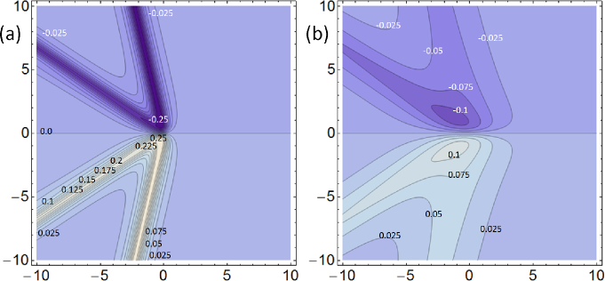
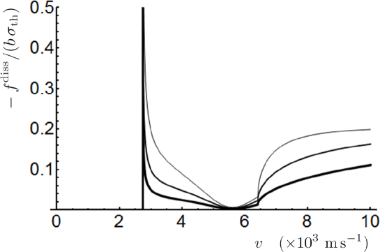
Fig. 3 displays the dependence on the fixed core width $a_{\parallel}$ of the dissipative force $f^{\rm diss}$, Equ. (38), which is of sign opposite to $v$. The overall dissipation decreases as the longitudinal core width increases. The figure illustrates several other aspects of the problem, among which the critical velocities $v_{1}=2.75\times 10^{3}$ m s^-1 at which the intersonic regime (with at least one Mach cone) begins, and $v_{3}=6.41\times 10^{3}$ m s^-1, at which the fully supersonic regime (with three Mach cones) begins; see Pellegrini (2017) for wave patterns. Notable variations of the dissipation occurs at these special velocities. The dissipation is zero in the subsonic range $v<v_{1}$, where the self-force does no work (Anderson et al., 2017). Indeed, a detailed study of Eqs. (31) would show that $\beta_{ij}(\mathbf{r}=\mathbf{0})$ vanishes in this regime. By contrast, even though $\sigma_{12}(\mathbf{r}=\mathbf{0})$ vanishes for all velocities (e.g., Figs. 1 and 2), other components of $\sigma_{ij}(\mathbf{r}=\mathbf{0})$ remain nonzero for $v>v_{1}$, which leads to finite dissipation via radiation in Mach cones. The force is minimal, of order $10^{-3}b\sigma_{\rm th}$ near to $v\simeq 5.6(1)\times 10^{3}$ m s^-1. This minimizer is quasi-independent of the ratio $a_{\parallel}/a_{\perp}$. Thus, the configuration is such that a ‘radiation-free’ velocity does not exist (Gao et al., 1999; Barnett and Zimmerman, 2002), but is replaced by a ‘least-radiation’ velocity. We speculate that the concept of a ‘least-radiation’ velocity is always applicable.

VI Concluding discussion

The proposed regularization allows for computations of the fields in an anisotropic medium, for a core with elliptical shape, in terms of closed-form expressions involving elementary functions and quantities accessible numerically from the Stroh formalism. The method delivers smooth, non-singular, field expressions that apply to any velocity, thus encompassing the supersonic domain at no additional price. The numerical results illustrate the dramatic effect of changing the core width on the intensity of the field, which is an important issue for dislocation-dynamics simulations, especially with regard to field-triggered nucleation processes. Obtaining the radiative force is immediate if the core width is fixed. This force is a fundamental piece of the steady-state stress-velocity law for dislocations (Rosakis, 2001). However, an ingredient is missing to complete the present theory, namely, the dependence in the velocity of the longitudinal core width $a_{\parallel}$. In principle, such a function $a_{\parallel}(v)$ could be deduced from a steady-state version of the method of Pellegrini (2014) to derive equations of motion for dislocations. A current physical limitation of the approach is that the functional form of the dislocation density is postulated rather than computed (in particular, this form might not be fully suited to supersonic motion). This should be contrasted with the markedly different field theory with gradient elasticity and quadratic core energy term (Lazar, 2009), which yields an equation for the dislocation density with Lorentz-Fitzgerald core contraction effects included. In this connection, the existence of Eq. (8) to produce the postulated dislocation density might provide a bridge between both approaches. These issues are left to future work.

Appendix A Angular integrals

A.1 Integrals (28c) and (28f)

The integrands are continuous functions of $\phi$, and the integrals are computed componentwise by contour integration on $\Gamma$, the unit circle $|z|=1$, by means of the change of variables $z=\mathrm{e}^{\mathrm{i}\phi}$, and the formula

$$\int_{0}^{2\pi}\frac{\mathrm{d}\phi}{2\pi}f(\phi)=\frac{1}{2\mathrm{i}\pi}\int_{\Gamma}\frac{\mathrm{d}z}{z}f(-\mathrm{i}\log z)=\sum_{\text{poles }|z_{k}|<1}\text{Res }g(z)|_{z=z_{k}},$$ (40)

where $g(z)=f(-\mathrm{i}\log z)/z$. The integrands in integrals (28c) have 5 poles $z_{k}$, $k=1,\ldots,5$, and those in (28f) have two more poles $z_{6,7}$. These are

$$z_{1} =0,z_{2,3}=\pm\mathrm{e}^{\mathrm{i}\gamma}\left(\sqrt{1+\varepsilon^{2}}-\varepsilon\right),z_{4,5}=\pm\mathrm{e}^{\mathrm{i}\gamma}\left(\sqrt{1+\varepsilon^{2}}+\varepsilon\right),z_{6,7}=\pm\sqrt{\frac{p-\mathrm{i}}{p+\mathrm{i}}},$$ (41)

where $p=\tan\psi$. Thus, $|z_{2,3}|<1$, $|z_{4,5}|>1$, and $|z_{6,7}|<1$ if $\mathop{\mathrm{Im}}p>0$, and $|z_{6,7}|>1$ if $\mathop{\mathrm{Im}}p<0$.

For integral (28c) the integrand reads

$$\frac{1}{z}\frac{\sin(\gamma-\phi)}{\sin^{2}(\gamma-\phi)+\varepsilon^{2}}\left(\begin{array}[]{c}\cos\phi\\ \sin\phi\end{array}\right) =-\mathrm{i}\frac{\mathrm{e}^{\mathrm{i}\gamma}\left(z^{2}-\mathrm{e}^{2\mathrm{i}\gamma}\right)}{\prod_{k=1}^{5}(z-z_{k})}\left(\begin{array}[]{c}1+z^{2}\\ \mathrm{i}(1-z^{2})\end{array}\right)\equiv g(z).$$ (46)

Only the poles $z_{1,2,3}$ contribute to the result. Residues are denoted as $R^{m}_{k}$ for the $\mathbf{m}$ component and $R^{n}_{k}$ for the $\mathbf{n}$ component. The shorthand notation $X=\varepsilon/\sqrt{1+\varepsilon^{2}}$ is used hereafter. From (46) one gets

$$R_{1}^{m} =\mathrm{i}(\cos\gamma-\mathrm{i}\sin\gamma),\qquad R^{m}_{2,3}=-\frac{\mathrm{i}}{2}\left(\cos\gamma-\mathrm{i}\,X\sin\gamma\right),$$ (47a)

$$R_{1}^{n} =-(\cos\gamma-\mathrm{i}\sin\gamma),\qquad R^{n}_{2,3}=\frac{1}{2}\left(X\cos\gamma-\mathrm{i}\sin\gamma\right).$$ (47b)

By (40) the results are of the type $R_{1}+R_{2}+R_{3}=R_{1}+2R_{2}$ for both components, which leads to (29a).

For integral (28f) the integrand reads

$$\frac{1}{z}\frac{\sin(\gamma-\phi)\tan(\psi-\phi)}{\sin^{2}(\gamma-\phi)+\varepsilon^{2}}\left(\begin{array}[]{c}-\sin\phi\\ \cos\phi\end{array}\right)$$ (50)

$$\hskip 56.9055pt{}=\frac{\mathrm{e}^{\mathrm{i}\gamma}\left(z^{2}-\mathrm{e}^{2\mathrm{i}\gamma}\right)}{\prod_{k=1}^{7}(z-z_{k})}\left(z^{2}+\frac{p-\mathrm{i}}{p+\mathrm{i}}\right)\left(\begin{array}[]{c}-\mathrm{i}(1-z^{2})\\ 1+z^{2}\end{array}\right)\equiv g(z).$$ (53)

Only the poles $z_{1,2,3,6,7}$ contribute. The residues deduced from (53) are

$$R^{m}_{1} =-\mathrm{i}(\cos\gamma-\mathrm{i}\sin\gamma),\qquad R^{m}_{6,7}=\frac{\mathrm{i}(\cos\gamma+p\sin\gamma)}{D_{\gamma\varepsilon}(p)},$$ (54a)

$$R^{m}_{2,3} =\frac{\mathrm{i}}{2}\left(\cos\gamma-\mathrm{i}\,X\sin\gamma\right)+\frac{-(pX+\mathrm{i})\cos\gamma+(X-\mathrm{i}\,p)\sin\gamma}{2D_{\gamma\varepsilon}(p)},$$ (54b)

and

$$R^{n}_{1} =\mathrm{i}\,R^{m}_{1},\qquad R^{n}_{6,7}=p\,R^{m}_{6,7}$$ (54c)

$$R^{n}_{2,3} =-\frac{1}{2}\left(X\cos\gamma-\mathrm{i}\,\sin\gamma\right)+p\frac{-(pX+\mathrm{i})\cos\gamma+(X-\mathrm{i}\,p)\sin\gamma}{2D_{\gamma\varepsilon}(p)},$$ (54d)

where $D_{\gamma\varepsilon}(p)$ is defined in (30a). By (40), and given the locations of the poles, the results are of the type $R_{1}+R_{2}+R_{3}=R_{1}+2R_{2}$ if $\mathop{\mathrm{Im}}p<0$, and $R_{1}+R_{2}+R_{3}+R_{6}+R_{7}=R_{1}+2R_{2}+2R_{6}$ if $\mathop{\mathrm{Im}}p>0$, which can be encoded as $R_{1}+2R_{2}+R_{6}+\mathop{\text{sign}}(\mathop{\mathrm{Im}}p)R_{6}$. Immediate simplifications then lead to (29b).

A.2 Integral (28i)

The integrand of (28i) is invariant under the symmetry $\phi\to\phi+\pi$. The integral is folded onto the interval $[0,\pi]$ where $\mathop{\text{sign}}(\sin\phi)=1$, which eliminates this factor. The change of variables $z=\tan(\phi/2)$ (Cartan, 1995) is used thereafter. Thus,

$$\left\langle\frac{\tan(\psi-\phi)\mathop{\text{sign}}(\sin\phi)}{\sin^{2}(\gamma-\phi)+\varepsilon^{2}}\left(\begin{array}[]{c}\sin\phi\\ -\cos\phi\end{array}\right)\right\rangle_{\!\!\phi}=\int_{0}^{\pi}\frac{\mathrm{d}\phi}{\pi}\frac{\tan(\psi-\phi)}{\sin^{2}(\gamma-\phi)+\varepsilon^{2}}\left(\begin{array}[]{c}\sin\phi\\ -\cos\phi\end{array}\right)$$ (59)

$$=\frac{1}{\pi}\int_{0}^{+\infty}\mathrm{d}z\frac{2[p(z^{2}-1)+2z]}{(z^{2}-2p\,z-1)[(2z\cos\gamma+(z^{2}-1)\sin\gamma)^{2}+(1+z^{2})^{2}\varepsilon^{2}]}\left(\begin{array}[]{c}2z\\ z^{2}-1\end{array}\right).$$ (62)

Figure 4: Integration contour $\Gamma$ for integral (62), where the contour radius goes to infinity.

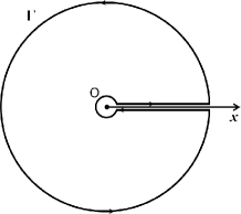
Integral (62) can then be computed as (Cartan, 1995)

$$\frac{1}{\pi}\int_{0}^{+\infty}\mathrm{d}z\,f(z) =-\frac{1}{\pi}\frac{1}{2\mathrm{i}\pi}\int_{\Gamma}\mathrm{d}z\,\log(-z)f(z)=-\frac{1}{\pi}\sum_{\text{poles }z_{k}}\mathop{\rm Res}f(z)_{z=z_{k}}\log(-z_{k}),$$ (63)

where $f(z)$ is the integrand in (62), and where the new contour $\Gamma$ is depicted in Fig. 4. The sum is over all the poles of $f(z)$ with nonzero imaginary part. The six poles of $f(z)$ are such, because in the modified Stroh formalism the $p_{\alpha}$ are always complex-valued due to the radiation condition; see Sec. III.4. They read

$$z_{1,2} =p\pm\sqrt{1+p^{2}},\quad z_{3,4}=-\frac{\cos\gamma\pm\sqrt{1+\varepsilon^{2}}}{\sin\gamma+\mathrm{i}\varepsilon},\quad z_{5,6}=-\frac{\cos\gamma\pm\sqrt{1+\varepsilon^{2}}}{\sin\gamma-\mathrm{i}\varepsilon}.$$ (64)

Let $s_{\gamma}(p)=\sin\gamma-p\cos\gamma$ and $c_{\gamma}(p)=\cos\gamma+p\sin\gamma$. The corresponding residues for both components of $f(z)$ are

$$R^{m}_{1,2} =\pm\frac{\sqrt{1+p^{2}}}{D_{\gamma\varepsilon}(p)},\qquad R^{n}_{1,2}=\pm\frac{p\,\sqrt{1+p^{2}}}{D_{\gamma\varepsilon}(p)},$$ (65a)

$$R^{m}_{3,4,5,6} =\pm\frac{1}{2\sqrt{1+\varepsilon^{2}}}\left(\sin\gamma+\frac{s_{\gamma}(p)}{D_{\gamma\varepsilon}(p)}\right)\pm\frac{\mathrm{i}}{2\varepsilon}\left(\cos\gamma-\frac{c_{\gamma}(p)}{D_{\gamma\varepsilon}(p)}\right),$$ (65b)

$$R^{n}_{3,4,5,6} =\pm\frac{1}{2\sqrt{1+\varepsilon^{2}}}\left(-\cos\gamma+p\frac{s_{\gamma}(p)}{D_{\gamma\varepsilon}(p)}\right)\pm\frac{\mathrm{i}}{2\varepsilon}\left(\sin\gamma-p\frac{c_{\gamma}(p)}{D_{\gamma\varepsilon}(p)}\right),$$ (65c)

where the residues $R_{3}$, $R_{4}$, $R_{5}$, and $R_{6}$ are defined, respectively, by the pairs of signs $(+,+)$, $(-,+)$, $(+,-)$, and $(-,-)$. Due to these alternating signs, the sum (63) involves the following combinations of logarithms, in which principal determinations of elementary functions are used:

$$\log(-z_{1})-\log(-z_{2})=2{\rm Arcsinh}(p)-\mathrm{i}\pi\mathop{\text{sign}}(\mathop{\mathrm{Im}}p),$$ (66a)

$$\log(-z_{3})-\log(-z_{4})+\log(-z_{5})-\log(-z_{6})=4{\rm Arctanh}\left(\frac{\cos\gamma}{\sqrt{1+\varepsilon^{2}}}\right),$$ (66b)

$$\log(-z_{3})+\log(-z_{4})-\log(-z_{5})-\log(-z_{6})=2\mathrm{i}{\rm Arg}\left((\varepsilon+\mathrm{i}\sin\gamma)^{2}\right).$$ (66c)

Re-organizing the sum (63) with the help of the above results and definitions (30b)–(30d) for each component immediately gives expression (29c).

References

- Anderson et al. (2017) Anderson, P. M., Hirth, J. P. and Lothe, J. [2017] Theory of Dislocations, 3rd ed. (Cambridge University Press, Cambridge).
- Auld (1973) Auld, B. A. [1973] Acoustic Fields and Waves, Vols. 1 and 2 (Wiley, New York).
- Bacon et al. (1979) Bacon, D. J., Barnett, D. M. and Scattergood, R. O. [1979] “Anisotropic continuum theory of lattice defects,” Progress in Materials Science 23, 51–262.
- Barnett and Zimmerman (2002) Barnett, D. M. and Zimmerman, J. A. [2002] “Nonradiating dislocations in uniform supersonic motion in anisotropic linear elastic solids,” in P. Schiavone, C. Constanda and A. Mioduchowski (eds.), Integral Methods in Science and Engineering (Birkhäuser, Boston), pp. 45–49.
- Barton (1989) Barton, G. [1989] Elements of Green’s Functions and Propagation — Potentials, Diffusion and Waves (Clarendon Press, Oxford).
- Blaschke and Szajewski (2018) Blaschke, D. N. and Szajewski, B. A. [2018] “Line tension of a dislocation moving through an anisotropic crystal,” Philosophical Magazine 98(26), 2397–2424.
- Bullough and Bilby (1954) Bullough, R. and Bilby, B. A. [1954] “Uniformly moving dislocations in anisotropic media,” Proceedings of the Physical Society B 67(8), 615–624.
- Cai et al. (2006) Cai, W., Arsenlis, A., Weinberger, C. R. and Bulatov, V. V. [2006] “A non-singular continuum theory of dislocations,” Journal of the Mechanics and Physics of Solids 54(3), 561–587.
- Cartan (1995) Cartan, H. [1995] Elementary Theory of Analytic Functions of One or Several Complex Variables (Dover, New York).
- Chadwick and Smith (1977) Chadwick, P. and Smith, G. D. [1977] “Foundations of the theory of surface waves in anisotropic elastic materials”, Advances in Applied Mechanics 17, 303–376.
- Eshelby (1949) Eshelby, J. D. [1949] “Uniformly moving dislocations,” Proceedings of the Physical Society A 62(5), 307–314.
- Eshelby (1953) Eshelby, J. D. [1953] “The equation of motion of a dislocation,” Physical Review 90(2), 248–255.
- Eshelby (1956) Eshelby, J. D. [1956] “Supersonic dislocations and dislocations in dispersive media,” Proceedings of the Physical Society B 69(10), 1013–1019.
- Gao et al. (1999) Gao, H., Huang, Y., Gumbsch, P. and Rosakis, A. J. [1999] “On radiation-free transonic motion of cracks and dislocations,” Journal of the Mechanics and Physics of Solids 47(9), 1941–1961.
- Jackson (1998) Jackson, J. D. [1998] Classical Electrodynamics, 3rd ed. (John Wiley & Sons, New York).
- Jacobsen (1989) Jacobsen, F. [1989] “Active and reactive, coherent and incoherent sound fields” Journal of Sound and Vibration 130(3), 493–507.
- Josien et al. (2018) Josien, M., Pellegrini, Y.-P., Legoll, F. and Le Bris, C. [2018] “Fourier-based numerical approximation of the Weertman equation for moving dislocations,” International Journal for Numerical Methods in Engineering 113(12), 1827–1850.
- Lazar (2009) Lazar, M. [2009] “The gauge theory of dislocations: a uniformly moving screw dislocation,” Proceedings of the Royal Society A 465(2108), 2505–2520.
- Lazar and Pellegrini (2016) Lazar, M. and Pellegrini, Y.-P. [2016] “Distributional and regularized radiation fields of non-uniformly moving straight dislocations, and elastodynamic Tamm problem,” Journal of the Mechanics and Physics of Solids 96, 632–659.
- Lazar and Po (2015a) Lazar, M. and Po, G. [2015a] “The non-singular Green tensor of gradient anisotropic elasticity of the Helmholtz type,” European Journal of Mechanics - A/Solids 50, 152–162.
- Lazar and Po (2015b) Lazar, M. and Po, G. [2015b] “The non-singular Green tensor of Mindlin’s anisotropic gradient elasticity with separable weak non-locality,” Physics Letters A 379(24–25), 1538–1543.
- Lide (2010) Lide, D. R. (ed.) [2010] CRC Handook of Chemistry and Physics (CRC Press/Taylor and Francis, Boca Raton, FL.).
- Lothe (1992) Lothe, J. [1992] “Uniformly moving dislocations; surface waves”, in V.L. Indenbom and J. Lothe (eds.), Elastic strain fields and dislocation mobility (North-Holland, Amsterdam), pp. 447–487.
- Markenscoff and Ni (2001a) Markenscoff, X. and Ni, L. [2001a] “The transient motion of a dislocation with a ramp-like core,” Journal of the Mechanics and Physics of Solids49(7), 1603–1619.
- Markenscoff and Ni (2001b) Markenscoff, X. and Ni, L. [2001b] “The transient motion of a ramp-core supersonic dislocation,” ASME Journal of Applied Mechanics 68(4), 656–659.
- Mura (1987) Mura, T. [1987] Micromechanics of defects in solids (Martinus Nijhoff Publishers, Dordrecht).
- Nabarro (1947) Nabarro, F. R. N. [1947] “Dislocations in a simple cubic lattice,” Proceedings of the Physical Society 59(2), 256–272.
- Peierls (1940) Peierls, R. [1940] “The size of a dislocation,” Proceedings of the Physical Society 52(1), 34–37.
- Pellegrini (2010) Pellegrini, Y.-P. [2010] “Dynamic Peierls-Nabarro equations for elastically isotropic crystals,” Phys. Rev. B 81(2), 024101.
- Pellegrini (2012) Pellegrini, Y.-P. [2012] “Screw and edge dislocations with time-dependent core width: From dynamical core equations to an equation of motion,” Journal of the Mechanics and Physics of Solids 60(2), 227–249.
- Pellegrini (2014) Pellegrini, Y.-P. [2014] “Equation of motion and subsonic-transonic transitions of rectilinear edge dislocations: A collective-variable approach,” Physical Review B 90(5), 054120.
- Pellegrini and Lazar (2015) Pellegrini, Y.-P. and Lazar, M. [2015] “On the gradient of the Green tensor in two-dimensional elastodynamic problems, and related integrals: Distributional approach and regularization, with application to nonuniformly moving sources,” Wave Motion 57, 44–63.
- Pellegrini (2017) Pellegrini, Y.-P. [2017] “Causal Stroh formalism for uniformly-moving dislocations in anisotropic media: Somigliana dislocations and mach cones,” Wave Motion 68, 128–148.
- Po et al. (2018) Po, G., Lazar, M., Admal, N. C. and Ghoniem, N. [2018] “A non-singular theory of dislocations in anisotropic crystals,” International Journal of Plasticity 103, 1–22.
- Rosakis (2001) Rosakis, P. [2001] “Supersonic dislocation kinetics from an augmented Peierls model,” Physical Review Letters 86(1), 95–98.
- Sáenz (1953) Sáenz, A. W. [1953] “Uniformly moving dislocations in anisotropic media,” Journal of Rational Mechanics and Analysis 2(1), 83–98.
- Schoeck (2005) Schoeck, G. [2005] “The Peierls model: progress and limitations,” Material Science and Engineering A 400–401, 7–17.
- Stroh (1962) Stroh, A. N. [1962] “Steady state problems in anisotropic elasticity,” Journal of Mathematics and Physics (Cambridge, MA) 41(1–4), 77–103.
- Teutonico (1962) Teutonico, L. J. [1962] “Uniformly moving dislocations of arbitrary orientation in anisotropic media,” Physical Review 127(2), 413–418.
- Weertman (1967) Weertman, J. [1967] “Uniformly moving transonic and supersonic dislocations,” Journal of Applied Physics 38(13), 5293–5301.
- Weertman (1969a) Weertman, J. [1969a] “Dislocations in uniform motion on slip or climb planes having periodic force laws,” in T. Mura (ed.), Mathematical Theory of Dislocations (American Society of Mechanical Engineers, New York), pp. 178–202.
- Weertman (1969b) Weertman, J. [1969b] “Stress dependence on the velocity of a dislocation moving on a viscously damped slip plane,” in A. Argon (ed.), Physics of Strength and Plasticity (The M.I.T. Press, Cambridge, MA.), pp. 75–83.
- Weertman and Weertman (1980) Weertman, J. and Weertman, J. R. [1980] “Moving dislocations,” in F. R. N. Nabarro (ed.), Dislocations in Solids, Vol. 3: Moving Dislocations, Dislocations in Solids, Vol. 3, chap. 8 (North-Holland, Amsterdam), pp. 1–60.
- Wu (2000) Wu, K.-C. [2000] “Extension of Stroh’s formalism to self-similar problems in two-dimensional elastodynamics,” Proceedings of the Royal Society A 456, 869–890.