Recommendation Through Mixtures
of Heterogeneous Item Relationships

Abstract.

Recommender Systems have proliferated as general-purpose approaches to model a wide variety of consumer interaction data. Specific instances make use of signals ranging from user feedback, item relationships, geographic locality, social influence (etc.). Typically, research proceeds by showing that making use of a specific signal (within a carefully designed model) allows for higher-fidelity recommendations on a particular dataset. Of course, the real situation is more nuanced, in which a combination of many signals may be at play, or favored in different proportion by individual users. Here we seek to develop a framework that is capable of combining such heterogeneous item relationships by simultaneously modeling (a) what modality of recommendation is a user likely to be susceptible to at a particular point in time; and (b) what is the best recommendation from each modality. Our method borrows ideas from mixtures-of-experts approaches as well as knowledge graph embeddings. We find that our approach naturally yields more accurate recommendations than alternatives, while also providing intuitive ‘explanations’ behind the recommendations it provides.

1. Introduction

Understanding, predicting, and recommending activities means capturing the dynamics of a wide variety of interacting forces: users’ preferences (Koren et al., 2009; Rendle et al., 2009), the context of their behavior (e.g. their location (Yang et al., 2017; Liu et al., 2013; Feng et al., 2015), their role in their social network (Zhao et al., 2014; Wu et al., 2017; Shu et al., 2018), their dwell time (Yi et al., 2014; Beutel et al., 2018), etc.), and the relationships between the actions themselves (e.g. which actions tend to co-occur (Koren, 2008; Kabbur et al., 2013), what are their sequential dynamics (Rendle et al., 2010; He and McAuley, 2016; Tang and Wang, 2018), etc.). Recommender Systems are a broad class of techniques that seek to capture such interactions by modeling the complex dynamics between users, actions, and their underlying context.

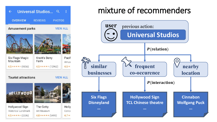
Figure 1. A demonstration of our approach. We model recommendations as a probabilistic mixture over several heterogeneous item-to-item recommenders; when making a recommendation to a user we must then model what types of relations they’re likely to adopt, as well as the relation-specific recommendations themselves. The relation types can either be manually engineered or automatically extracted from data.

A dominant paradigm of research says that actions can be accurately modeled by explaining interactions between users and items, as well as interactions between items and items. User-to-item interactions might explain users’ preferences or items’ properties, while item-to-item interactions might describe similarity or contextual relationships between items. Examples of such models include Factorized Personalized Markov Chains (FPMC) (Rendle et al., 2010) which capture user-to-item and item-to-item interactions via low-rank matrix decomposition, or more recent approaches such as TransRec (He et al., 2017a) or CKE (Zhang et al., 2016) which seek to capture similar ideas using knowledge-graph embedding approaches.

Within these frameworks, research often proceeds by positing new types of user-to-item or item-to-item relationships that increase recommendation fidelity on a particular dataset, e.g.  geographical similarities help POI recommendation (Yang et al., 2017), “also-viewed” products help rating prediction (Park et al., 2017), etc. Each of these assumptions is typically associated with a hand-crafted model which seeks to capture the relationship in detail.

In this paper we seek a more general-purpose approach to describing user-to-item and item-to-item relationships. Essentially, we note that real action sequences in any given setting simultaneously depend on several types of relationships: at different times a user might select an item based on geographical convenience, her personal preferences, the advice of her friends, or some combination of these (Figure 1); different users may weight these forms of influence in different proportions. Thus we seek a model that learns personalized mixtures over the different ‘reasons’ why users may favor a certain action at a particular point in time.

We capture this intuition with a new model—Mixtures of Heterogeneous Recommenders (MoHR). Methodologically, MoHR models sequential recommendation problems in terms of a long-term preference recommender as well as a personalized, probabilistic mixture of heterogeneous item-to-item recommenders. Our method is built upon recent approaches that model recommendation in terms of translational metric embeddings (Bordes et al., 2013; He et al., 2017a; Tay et al., 2018; Garcia-Duran et al., 2018), though in principle our model is a general framework that could be applied to any model-based recommendation approach.

We compare MoHR against various state-of-the-art recommendation methods on multiple existing and new datasets from real applications including Amazon, Google Local, and Steam. Our results show that MoHR can generate more accurate recommendations in terms of both overall and top-n ranking performance.

2. Related Work

General Recommendation. Conventional approaches to recommendation model historical traces of user-item interactions, and at their core seek to capture users’ preferences and items’ properties. Collaborative Filtering (CF) and especially Matrix Factorization (MF) have become popular underlying approaches (Koren et al., 2009). Due to the sparsity of explicit feedback (e.g. rating) data, MF-based approaches have been proposed that make use of implicit feedback data (like clicks, check-ins, and purchases) (Hu et al., 2008). This idea has been extended to optimize personalized rankings of items, e.g. to approximately optimize metrics such as the AUC (Rendle et al., 2009). A recent thrust in this direction has shown that the performance of such approaches can be improved by modeling latent embeddings within a metric space (Hsieh et al., 2017; Tay et al., 2018; Chen et al., 2012). Although our approach is a general purpose framework that in principle could be adapted to any (model-based) recommenders, we make use of metric-learning approaches due to their strong empirical performance.

Temporal and Sequential Recommendation. The timestamps, or more simply the sequence, of users’ actions provide important context to generate more accurate recommendations. For example, TimeSVD++ sought to exploit temporal signals (Koren, 2010), and was among the state-of-the-art methods on the Netflix prize. Often simply knowing the sequence of items (i.e., their ordering), and in particular the previous action by a user, is enough to estimate their next action, especially in sparse datasets. Sequential models often decompose the problem into two parts: user preference modeling and sequential pattern modeling (Rendle et al., 2010; Feng et al., 2015). Factorized Personalized Markov Chain (FPMC) (Rendle et al., 2010) is a classic sequential recommendation model that fuses MF (to model user preferences) and factorized Markov Chains (to model sequential patterns). Recently, inspired by translational metric embeddings (Bordes et al., 2013), sequential recommendation models have been combined with metric embedding approaches. In particular, TransRec unifies the two parts by modeling each user as a translating vector from her last visited item to the next item (He et al., 2017a).

Neural Recommender Systems. Various deep learning techniques have been introduced for recommendation (Zhang et al., 2017). One line of work seeks to use neural networks to extract item features (e.g. images (Wang et al., 2017; Kang et al., 2017), text (Wang et al., 2015; Kim et al., 2016), etc.) for content-aware recommendation. Another line of work seeks to replace conventional MF. For example, NeuMF (He et al., 2017b) estimates user preferences via Multi-Layer Perceptions (MLPs), and AutoRec (Sedhain et al., 2015) predicts ratings using autoencoders. In particular, for modeling sequential user behavior, Recurrent Neural Networks (RNNs) have been adopted to capture item transition patterns in sequences  (Hidasi et al., 2016; Jing and Smola, 2017; Smirnova and Vasile, 2017; Li et al., 2017; Pei et al., 2017). In addition, CNN-based approaches have also shown competitive performance on sequential and session-based recommendation (Tang and Wang, 2018; Tuan and Phuong, 2017).

‘Relationship-aware’ Recommendation. The recommendation methods described above learn user and item embeddings from user feedback. To overcome the sparsity of user feedback, some methods essentially seek to ‘regularize’ item embeddings based on item similarities or item relationships. For example the POI recommendation method PACE (Yang et al., 2017) learns user and item representations while seeking to preserve item-to-item similarities based on geolocation. Amazon product recommendations have also benefited from the use of “also-viewed” products in order to improve rating prediction (Park et al., 2017); again relations among items essentially act as a form of regularizer that constrains item embeddings. These ideas are especially useful in ‘cold-start’ scenarios, where information from related items mitigates the sparsity of interactions with new items. To exploit complex relationships, a line of work extracts item features from manually constructed meta-paths or meta-graphs in Heterogeneous Information Networks (HIN) (Yu et al., 2014; Zhao et al., 2017). Our method is closer to another line of work, like CKE (Zhang et al., 2016), which uses knowledge graph embedding techniques to automatically learn semantic item embeddings from heterogeneous item relationships.

Knowledge Graph Embeddings. Originating from knowledge base domains which focus on modeling multiple, complex relationships between various entities, translating embeddings (e.g. TransE (Bordes et al., 2013) and TransR (Lin et al., 2015)) have achieved state-of-the-art accuracy and scalability. Other than methods like Collaborative Knowledge Base Embedding (CKE) (Zhang et al., 2016) which use translating embeddings as regularization, several translation-based recommendation models have been proposed (e.g. TransRec (He et al., 2017a), LRML (Tay et al., 2018), TransRev (Garcia-Duran et al., 2018)), which show superior performance on various recommendation tasks. Our model also adopts the translational principle to model heterogeneous interactions among users, items and relationships.

Table 1. Notation.

Notation	Description
$\mathcal{U},\mathcal{I}$	user and item set
$\mathcal{S}^{u}$	historical interaction sequence for a user $u$: $(\mathcal{S}^{u}_{1},\mathcal{S}^{u}_{2},...,\mathcal{S}^{u}_{|\mathcal{S}^{u}|})$
$\mathcal{R}$	item relationship set: $\{r_{1},r_{2},...,r_{|\mathcal{R}|}\}$
$\mathcal{\hat{R}}$	$\mathcal{\hat{R}}=\mathcal{R}\bigcup\{r_{0}\}$, where $r_{0}$ stands for a latent relationship
$\mathcal{I}_{i,r}$	item set includes all items having relation $r\in\mathcal{R}$ with item $i$
$K\in\mathbb{N}$	latent vector dimensionality
${\bm{\theta}}_{u}\in\mathbb{R}^{K}$	latent vector for user $u$ where $u\in\mathcal{U}$
${\bm{\theta}}_{i}\in\mathbb{R}^{K}$	latent vector for item $i$ where $i\in\mathcal{I}$
${\bm{\theta}}_{r}\in\mathbb{R}^{K}$	latent vector for relation $r$ where $r\in\mathcal{\hat{R}}$
$b_{i}\in\mathbb{R}$	bias term for item $i$ where $i\in\mathcal{I}$
$b_{r}\in\mathbb{R}$	bias term for relation $r$ where $r\in\mathcal{\hat{R}}$
$d(x,y)$	squared $\mathcal{L}_{2}$-distance between point $x$ and $y$
$[n]$	set of natural numbers less or equal than $n$

3. MoHR: Mixtures of Heterogeneous Recommenders

Our model builds on a combination of two ideas: (1) to build item-to-item recommendation approaches by making use of the translational principle (inspired by methods such as (Bordes et al., 2013; He et al., 2017a; Zhang et al., 2016)), followed by (2) to learn how to combine several sources of heterogeneous item-to-item relationships in order to fuse multiple ‘reasons’ that users may follow at a particular time point. Following this we show how to combine these ideas within a sequential recommendation framework, and discuss parameter learning, model complexity, etc. Our notation is summarized in Table 1.

3.1. Modeling Item-to-Item Relationships

Item-to-item recommendation consists of identifying items related to one a user has recently interacted with, or is currently considering. What types of items are related is platform-dependent and will vary according to the domain characteristics of items. Relationships can be heterogeneous, since two items may be related because they are similar in different dimensions (e.g. function, category, style, location, etc.) or complementary. Some work seeks to exploit one or two specific relationship(s) to improve recommendations, such as recent works that consider ‘also-viewed’ products (Park et al., 2017) or geographical similarities (Yang et al., 2017). Extending this idea, we seek to use a general method to model such recommendation problems with heterogeneous relationships, improving its performance while making it easily adaptable to different domains. As we show, this approach can be applied to model a small number of hand-selected relationship types, or a large number of automatically extracted item-to-item relationships.

Specifically, for a given item $i$ and a relationship type $r$, we consider ‘related-item’ lists containing items that exhibit relationship $r$ with item $i$ (e.g. ‘also viewed’ links for an item $i$). This can equivalently be thought of as a (directed) multigraph whose edges link items via different relationship types.

Using these relationships we define a recommender to model the interaction between the three elements (two items $i$ and $i^{\prime}$ linked via a relationship $r$) using a translational operation (Bordes et al., 2013):

(1) $$R(i^{\prime}|i,r)=b_{i^{\prime}}-d({\bm{\theta}}_{i}+{\bm{\theta}}_{r},{\bm{\theta}}_{i^{\prime}}),$$

where $b_{i^{\prime}}$ is a bias term. This idea is drawn from knowledge graph embedding techniques where two entities (e.g. $i=\text{Alan Turing}$ and $i^{\prime}=\text{England}$) should be ‘close to’ each other under a certain relation operation (e.g. $r=\text{Born in}$). When used to model (e.g.) sequential relationships among items, such models straightforwardly combine traditional recommendation approaches with the translational principle (He et al., 2017a). This idea has also been applied to several recommendation tasks and achieves strong performance (He et al., 2017a; Tay et al., 2018; Garcia-Duran et al., 2018).

Similar to Bayesian Personalized Ranking (Rendle et al., 2009), we minimize an objective contrasting the score of related ($i^{\prime}$) versus not-related ($i^{\text{-}}$) items:

(2) $$T_{I}=-\sum_{(i,r,i^{\prime},i^{\text{-}})\in\mathcal{D}_{I}}\ln\sigma(R(i^{\prime}|i,r)-R(i^{\text{-}}|i,r)),$$

where

$$\mathcal{D}_{I}=\{(i,r,i^{\prime},i^{\text{-}})|i\in\mathcal{I}\land r\in\mathcal{R}\land i^{\prime}\in\mathcal{I}_{i,r}\land i^{\text{-}}\in\mathcal{I}-\mathcal{I}_{i,r}\}.$$

The above objective encourages relevant items $i^{\prime}$ to be ranked higher (i.e., larger $R(i^{\prime}|i,r)$) than irrelevant items $i^{\text{-}}$ given the context of the item $i$ and relation $r$. Later we use the recommender $R(i^{\prime}|i,r)$ to evaluate how closely $i$ and $i^{\prime}$ are related in terms of a particular relation $r$. The recommender can also be used for inferring missing relations (as in e.g. (McAuley et al., 2015a)), however doing so is not the focus of this paper and we only use the structural information as side features as in (Park et al., 2017; Yang et al., 2017; Zhang et al., 2016).

3.2. Next-Relationship Prediction

Existing item-to-user recommendation methods typically only consider item-level preferences. However, many applications provide multiple types of related items, e.g. different types of co-occurrence links (also-viewed/also-bought/etc.). Here we seek to model the problem of predicting which type of relationship a user is most likely to follow for their next interaction. All items that a user selects are presumed to be related to previous items the user has interacted with, either via explicit relationships or via latent transitions. For example, when selecting a POI to visit (as in fig. 1), a user may prefer somewhere nearby their current POI, similar to, or complementary to their current POI. Thus a more effective recommender system might be designed by learning to estimate which ‘reason’ for selecting a recommendation a user will pursue at a particular point in time.

By making use of users’ sequential feedback and item-to-item relationships, we can define the relevant relationships $\tau(u,k)$ given the context of the user $u$ and the $k$-th item $\mathcal{S}^{u}_{k}$ from her feedback sequence $\mathcal{S}^{u}$:

$$\begin{split}\tau(u,k)=\left\{\begin{array}[]{lr}\{r_{0}\}&\forall_{r\in\mathcal{R}},\ \mathcal{S}^{u}_{k+1}\notin\mathcal{I}_{\mathcal{S}^{u}_{k},r}\\ \{r|\mathcal{S}^{u}_{k+1}\in\mathcal{I}_{\mathcal{S}^{u}_{k},r}\land r\in\mathcal{R}\}&\text{otherwise}\\ \end{array}\right..\end{split}$$

The first condition in $\tau$ means that if two consecutive items share no relationship, the relevant relationship becomes a ‘latent’ relationship $r_{0}$, which accounts for transitions that cannot be explained by any explicit relationship. Otherwise, shared relationships are relevant. Then, similarly, we define a translation-based recommender to model the interaction between the three elements:

(3) $$R(r|u,i)=b_{r}-d({\bm{\theta}}_{u}+{\bm{\theta}}_{i},{\bm{\theta}}_{r}).$$

Note that in contrast to eq. 1—which predicts the next item under a given relationship—eq. 3 predicts which relationship will be selected following the previous item.

In particular, we define a probability function $P$ over all relationships (including $r_{0}$). The relevance between the relationship $r$ and context $(u,i)$ is represented by

(4) $$P(r|u,i)=\frac{\exp(R(r|u,i))}{\sum_{r^{\prime}\in\mathcal{\hat{R}}}\exp(R(r^{\prime}|u,i))}.$$

Again we optimize the ranking between relevant and irrelevant relationships by minimizing

(5) $$T_{R}=-\sum_{(u,i,r,r^{\text{-}})\in\mathcal{D}_{R}}\ln\sigma(P(r|u,i)-P(r^{\text{-}}|u,i)),$$

where

$$\mathcal{D}_{R}=\{(u,\mathcal{S}^{u}_{k},r,r^{\text{-}})|u\in\mathcal{U}\land\\ k\in[|\mathcal{S}^{u}|-1]\land r\in\tau(u,k)\land r^{\text{-}}\in\mathcal{\hat{R}}-\tau(u,k)\}.$$

In addition to improving recommendations, we envisage that such a ‘relation type’-level recommender can be used in personalized layout ranking, e.g. on the webpage of an item, we might order or organize the types of related items shown to different users according to their preferences.

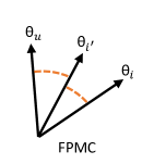
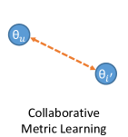
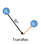
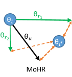
Figure 2. A simplified illustration of recommendation models in existing methods. The first two models are based on inner product spaces while the following three are metric-based. The orange dashed lines indicate how a model calculates its preference score given a user $u$, her last visited item $i$ and next item $i^{\prime}$. The width of lines in MoHR indicates their weight according to $P(r|u,i)$. Note that relationship-aware methods MCF (Park et al., 2017) and CKE (Zhang et al., 2016) also adopt MF as their underlying model.

3.3. Sequential Recommendation

Like existing sequential recommenders (such as FPMC (Rendle et al., 2010) and PRME (Feng et al., 2015)), our sequential recommender is also defined by fusing users’ long-term preferences and short-term item transitions. However, rather than learning purely latent transitions, our recommendation model uses a mixture of explicit and latent item transitions. The mixture model is inspired by the ‘mixtures of experts’ framework (Jacobs et al., 1991), which probabilistically mixes the outputs of different (weak) learners by weighting each learner according to its relevance to a given input. In our context, each ‘learner’ is a relationship type whose relevance is predicted given a query item. The elegance of such a framework is that it is not necessary for all learners (relationships) to accurately handle all inputs; rather, they need only be accurate for those inputs where they are predicted to be relevant. Here the weights on each item transition are conditioned on a user $u$ and her last visited item $i$. Specifically we define $R^{*}(i^{\prime}|u,i)$ as:

$$\begin{split}&b_{i^{\prime}}-\overbrace{d({\bm{\theta}}_{i}+{\bm{\theta}}_{u},{\bm{\theta}}_{i^{\prime}})}^{\mathclap{\text{long-term preference}}}+\underbrace{P(r_{0}|u,i)R(i^{\prime}|i,r_{0})}_{\mathclap{\text{latent short-term transitions}}}+\overbrace{\sum_{r\in\mathcal{R}}P(r|u,i)R(i^{\prime}|i,r)}^{\mathclap{\text{explicit short-term transitions}}},\end{split}$$

Note that relation $r_{0}$ is a latent item relationship to capture item transitions that cannot be explained by explicit relationships. Unlike learning explicit relationships as in eq. 1, $r_{0}$ is learned from users’ sequential feedback. By unifying latent and explicit transitions, we can rewrite the recommender as:

(6) $$R^{*}(i^{\prime}|u,i)=R(i^{\prime}|u,i)+\sum_{r\in\mathcal{\hat{R}}}\overbrace{P(r|u,i)}^{\mathclap{\text{probability of choosing $r$ as the next relation}}}\times\underbrace{R(i^{\prime}|i,r)}_{\mathclap{\text{transition from $i$ to $i^{\prime}$ using relation $r$}\ \ \ \ }}.$$

Thus the item-to-item recommenders and the next-relationship recommender are naturally integrated into our sequential recommendation model $R^{*}$.

Finally, the goal of sequential recommendation is to rank the ground-truth next-item $i^{\prime}$ higher than irrelevant items; the loss function we use (known as S-BPR(Rendle et al., 2010)) is defined as:

(7) $$T_{S}=-\sum_{(u,i,i^{\prime},i^{\text{-}})\in\mathcal{D}_{S}}\ln\sigma(R^{*}(i^{\prime}|u,i)-R^{*}(i^{\text{-}}|u,i))\text{,}$$

where $\mathcal{D}_{S}=\{(u,\mathcal{S}^{u}_{k},\mathcal{S}^{u}_{k+1},i^{\text{-}})|u\in\mathcal{U}\land k\in[|\mathcal{S}^{u}|-1]\land i^{\text{-}}\in\mathcal{I}-\mathcal{S}^{u}\}$.

Figure 2 further illustrates how our method compares to alternative recommendation approaches.

3.4. Multi-Task Learning

Different from existing methods like CKE (Zhang et al., 2016) which introduce additional item embeddings to capture structural item information, we use a multi-task learning framework (Caruana, 1997) to jointly optimize all three tasks using shared variables within a unified translational metric space. Using shared variables can reduce the model size (see Table 2 for comparison) and avoid over-fitting. Furthermore, representing different kinds of translational relationships in a unified metric space can be viewed as a form of regularization that fuses different sources of data.

Specifically, we jointly learn the three tasks in a multi-task learning framework:

(8) $$\begin{split}\min_{\Theta}&\quad T=T_{S}+\alpha T_{I}+\beta T_{R}+\lambda(\sum_{i\in\mathcal{I}}b_{i}^{2}+\sum_{r\in\mathcal{\hat{R}}}b_{r}^{2})\\ \mathit{s.t.}&\quad\|{\bm{\theta}}_{u}\|_{2}\leq 1,\|{\bm{\theta}}_{i}\|_{2}\leq 1,\|{\bm{\theta}}_{r}\|_{2}\leq 1\\ &\quad\forall u\in\mathcal{U},i\in\mathcal{I},r\in\mathcal{\hat{R}}\end{split}$$

where $\alpha$ and $\beta$ are two hyper-parameters to control the trade-off between the main task $T_{S}$ and auxiliary tasks, and learnable variables $\Theta=\{{\bm{\theta}}_{u},{\bm{\theta}}_{i},{\bm{\theta}}_{r},b_{i},b_{r}\}$. We constrain the latent vectors to lie within a unit ball. This regularization doesn’t push vectors toward the origin like $\mathcal{L}_{2}$ regularization, and has been shown to be effective in both knowledge graph embedding methods (Bordes et al., 2013; Lin et al., 2015) and metric-based recommendation methods (He et al., 2017a; Hsieh et al., 2017; Tay et al., 2018). The bias terms are regularized by a square penalty with coefficient $\lambda$.

We outline the training procedure as follows:

1. Sample three batches from $\mathcal{D}_{S}$, $\mathcal{D}_{I}$ and $\mathcal{D}_{R}$, respectively

2. Update parameters using an Adam (Kingma and Ba, 2014) optimizer for objective $T$ with the three batches

3. Censor the norm for all ${\bm{\theta}}_{u},{\bm{\theta}}_{i},{\bm{\theta}}_{r}$ by ${\bm{\theta}}={\bm{\theta}}/\max(\|{\bm{\theta}}\|_{2},1)$

4. Repeat this procedure until convergence

When $\alpha=0$, we don’t have semantic constraints on $R(i^{\prime}|i,r)$, meaning that all relationships become latent relationships. When $\beta=0$, we don’t have a prior on choosing the next relationship, meaning the model would optimize $P(r|u,i)$ only to fit sequential feedback. Typically we need to choose appropriate $\alpha>0$, $\beta>0$ to achieve satisfactory performance on the main task $T_{S}$. We discuss our hyper-parameter selection strategy in Section 4.

3.5. Complexity Analysis

The space complexity of MoHR can be calculated by the number of parameters: $(|\mathcal{U}|+|\mathcal{I}|+|\mathcal{R}|+1)*K+|\mathcal{I}|+|\mathcal{R}|+1$. Typically $|\mathcal{R}|$ is small, e.g. $|\mathcal{R}|=2\sim 101$ in the datasets we consider. Compared to CKE (Zhang et al., 2016) which assigns each item two $K$-dimensional factors, our model saves $|I|*K$ parameters; compared to TransRec whose model size is $(|\mathcal{U}|+|\mathcal{I}|)*K+|\mathcal{I}|$, our method only adds a modest number of parameters to model more information and tasks. The compactness of our model is mainly due to the sharing of parameters across tasks. Table 2 shows an empirical comparison of the number of model parameters of various methods.

The time complexity of the training procedure is $O(NBK|\mathcal{R}|)$, where $N$ is the number of iterations and $B$ represents the batch size. At test time, the time complexity of evaluating $R^{*}(i^{\prime}|u,i)$ is $O(K|\mathcal{R}|)$, which is larger than other methods (typically $O(K)$). However, $|\mathcal{R}|$ is typically small and our model computation (in both training and testing time) can be efficiently accelerated using multi-core CPUs or GPUs with our TensorFlow implementation.

3.6. Discussion of Related Methods

We examine two types of related methods and highlight the significance of our method through comparisons against them.

Sequential Recommendation Models. We compare our method with existing next-item recommendation methods, absent any item relationships (i.e, $\mathcal{R}=\{\}$). Here our recommender would become:

$$R^{*}_{0}(i^{\prime}|u,i)=b_{i^{\prime}}-d({\bm{\theta}}_{i}+{\bm{\theta}}_{u},{\bm{\theta}}_{i^{\prime}})-d({\bm{\theta}}_{i}+{\bm{\theta}}_{r_{0}},{\bm{\theta}}_{i^{\prime}}).$$

FPMC (Rendle et al., 2010) combines matrix factorization with factorized first-order Markov chains to capture user preference and item transitions:

$$R_{\text{FPMC}}(i^{\prime}|u,i)=\langle{\bm{\theta}}_{u},{\bm{\theta}}^{(1)}_{i^{\prime}}\rangle+\langle{\bm{\theta}}^{(2)}_{i},{\bm{\theta}}^{(3)}_{i^{\prime}}\rangle.$$

Compared to FPMC, MoHR uses a single latent vector ${\bm{\theta}}_{i}$ to reduce model size and all vectors are placed in a unified metric space rather than separate inner-product-based spaces, which empirically leads to better generalization according to (He et al., 2017a; Hsieh et al., 2017).

Recently, TransRec was proposed in order to introduce knowledge graph embedding techniques into recommendations (He et al., 2017a). In TransRec, each user is modeled as a translation vector mapping her last visited item to the next item:

$$R_{\text{TransRec}}(i^{\prime}|u,i)=b_{i^{\prime}}-d({\bm{\theta}}_{i}+{\bm{\theta}}_{u},{\bm{\theta}}_{i^{\prime}}).$$

Our method can be viewed as an extension of TransRec in that we incorporate a translation vector $r_{0}$ to model latent short-term item transitions.

However, our model learns a personalized mixture of explicit and latent item transitions, which is one of the main contributions in this work.

Relationship-Aware Recommendation Models. PACE (Yang et al., 2017) and MCF (Park et al., 2017) are two recent methods that regularize item embeddings by factorizing a binary item-to-item similarity matrix ${\bf S}$, where ${\bf S}_{ij}=1$ means item $i$ and item $j$ are similar (0 otherwise). Their item embedding is used for recommendation and factorizing ${\bf S}$, which essentially is a form of multi-task learning.

Unlike the two methods above which only consider homogeneous similarity, CKE (Zhang et al., 2016) models heterogeneous item relationships with knowledge graph embedding techniques (Bordes et al., 2013; Lin et al., 2015). To regularize the model, CKE uses the item embedding $\tilde{{\bm{\theta}}}_{i}$ as a Gaussian prior on the recommended item embedding ${\bm{\theta}}_{i}$. Note that ${\bm{\theta}}_{i}$ lies in an inner product space for Matrix Factorization while $\tilde{{\bm{\theta}}}_{i}$ is in a translational metric space for preserving item relationships. Our method uses a unified metric space with the same translational operation to represent both preferences and relationships.

The underlying recommendation models in the three methods above are simple (e.g. inner product of a user embedding and an item embedding), while MoHR’s recommendation model directly considers users’ sequential behavior and mixtures of item transitions.

Table 2. Model comparison. P: Personalized? M: Metric-based? S: Sequentially-aware? R (H-R): Models (heterogeneous) item relationship? Model Size: The number of learnable parameters (estimated under Google Local with $K=10$).

Property	P	M	S	R	H-R	Model Size
PopRec						0
BPR-MF (Rendle et al., 2009)	✓					$99.99\%$
CML (Hsieh et al., 2017)	✓	✓				$94.41\%$
FPMC (Rendle et al., 2010)	✓		✓			$222.94\%$
TransRec (He et al., 2017a)	✓	✓	✓			$99.99\%$
PACE (Yang et al., 2017)	✓			✓		$150.15\%$
MCF (Park et al., 2017)	✓			✓		$150.15\%$
CKE (Zhang et al., 2016)	✓			✓	✓	$150.16\%$
MoHR	✓	✓	✓	✓	✓	$100\%$

4. Experiments

Table 3. Statistics of dataset after preprocessing (in ascending order of item density).

Dataset	#users
$|\mathcal{U}|$	#items
$|\mathcal{I}|$	#actions
$\sum_{u\in\mathcal{U}}|\mathcal{S}^{u}|$	#relationships $|\mathcal{R}|$	#related items
$\sum_{i\in\mathcal{I}}\sum_{r\in\mathcal{R}}|\mathcal{I}_{i,r}|$	avg. #actions /user	avg. #actions /item	avg. #related items /item
Amazon Automotive	34,315	40,287	183,567	4	1,632,467	5.35	4.56	40.52
Google Local	350,811	505,516	2,591,026	101	48,307,315	7.39	5.13	95.56
Amazon Toys	57,617	69,147	410,920	4	3,943,494	7.13	5.94	57.03
Amazon Clothing	184,050	174,484	1,068,972	4	2,927,534	5.81	6.12	16.78
Amazon Beauty	52,204	57,289	394,908	4	2,082,502	7.56	6.89	36.43
Amazon Games	31,013	23,715	287,107	4	1,030,990	9.26	12.11	43.47
Steam	334,730	13,047	4,213,117	2	111,487	12.59	322.92	8.55
Total	1.04M	0.88M	9.15M	-	60.04M	-	-	-

4.1. Datasets

We evaluate our method on seven datasets from three large-scale real-world applications. The datasets vary significantly in domain, variability, feedback sparsity, and relationship sparsity. All the datasets we used and our code are publicly available.

Amazon. A collection of datasets introduced in (McAuley et al., 2015b), comprising large corpora of reviews as well as multiple types of related items. These data were crawled from Amazon.com and span May 1996 to July 2014. Top-level product categories on Amazon are treated as separate datasets. We consider a series of large categories including ‘Automotive,’ ‘Beauty,’ ‘Clothing,’ ‘Toys,’ and ‘Games.’ This set of data is notable for its high sparsity and variability. Amazon surfaces four types of item relationships that we use in our model: ‘also viewed,’ ‘also bought,’ ‘bought together,’ and ‘buy after viewing.’

Google Local. A POI-based dataset (He et al., 2017a) crawled from Google Local which contains user reviews and POIs (with multiple fine-grained categories) distributed over five continents. To construct item relationships (e.g. similar businesses), we first extract the top 100 categories (e.g. restaurants, parks, attractions, etc.) according to their frequency. Then, for each POI, based on its categories, we construct “similar business” relationships like “nearby attraction,” “nearby park,” etc. We also construct one more relationship called “nearby popular places,” based on each POI’s geolocation and popularity. Therefore, we obtain 101 relationship types in total.

Steam. We introduce a new dataset crawled from Steam, a large online video game distribution platform. The dataset contains 2,567,538 users, 15,474 games and 7,793,069 English reviews spanning October 2010 to January 2018. For each game we extract two kinds of item-to-item relations. The first is “more like this,” based on similarity-based recommendations from Steam. The second are items that are “bundled together,” where a bundle provides a discount price for games in the same series, made by the same publisher, (etc.). Bundle data was collected from (Pathak et al., 2017). The dataset also includes rich information that might be useful in future work, like user’s play hours, pricing information, media score, category, developer (etc.).

We followed the same preprocessing procedure from (He et al., 2017a). For all datasets, we treat the presence of a review as implicit feedback (i.e., the user interacted with the item) and use timestamps to determine the sequence order of actions. We discard users and items with fewer than 5 related actions. For partitioning, we split the historical sequence $\mathcal{S}^{u}$ for each user $u$ into three parts: (1) the most recent action $\mathcal{S}^{u}_{|\mathcal{S}^{u}|}$ for testing, (2) the second most recent action $\mathcal{S}^{u}_{|\mathcal{S}^{u}|-1}$ for validation, and (3) all remaining actions for training. Hyperparameters in all cases are tuned by grid search using the validation set. Data statistics are shown in Table 3.

Table 4. Ranking results on different datasets under Setting-1 (higher is better). The number of latent dimensions $K$ for all comparison methods is set to 10. The best performance in each case is underlined. The last column shows the percentage improvement of over the strongest baseline.

Dataset	Metric	PopRec	BPR-MF	CML	FPMC	TransRec	PACE	MCF	CKE	MoHR	%Improv.
Amazon Automotive	AUC	0.6426	0.6313	0.6395	0.6414	0.6675	0.7233	0.7416	0.7341	0.8026	8.2%
	HR@10	0.3481	0.3323	0.3062	0.3210	0.3332	0.4015	0.4424	0.4335	0.5382	21.7%
	NDCG@10	0.2084	0.2003	0.1793	0.1981	0.2034	0.2371	0.2735	0.2607	0.3478	27.2%
Google Local	AUC	0.5811	0.7552	0.7676	0.7835	0.7915	0.7727	0.8560	0.8488	0.9330	9.0%
	HR@10	0.2454	0.5742	0.5571	0.5505	0.7103	0.5099	0.7231	0.7095	0.8532	18.0%
	NDCG@10	0.1380	0.4318	0.3995	0.4147	0.5400	0.3249	0.5484	0.5195	0.6091	11.1%
Amazon Toys	AUC	0.6641	0.6863	0.7070	0.7164	0.7273	0.7610	0.7892	0.7914	0.8422	6.4%
	HR@10	0.3601	0.3378	0.4015	0.4170	0.4474	0.4590	0.5277	0.5183	0.6061	14.9%
	NDCG@10	0.2048	0.1926	0.2437	0.2651	0.2890	0.2820	0.3348	0.3284	0.4151	24.0%
Amazon Clothing	AUC	0.6609	0.6500	0.6527	0.6715	0.7034	0.7083	0.7529	0.7394	0.7882	4.7%
	HR@10	0.3661	0.3502	0.3307	0.3478	0.3608	0.3590	0.4278	0.4299	0.4919	14.9%
	NDCG@10	0.2166	0.2064	0.1904	0.2076	0.2111	0.1984	0.2601	0.2561	0.3015	16.5%
Amazon Beauty	AUC	0.6964	0.6767	0.7029	0.6874	0.7328	0.7638	0.7885	0.7805	0.8150	3.4%
	HR@10	0.4003	0.3761	0.4070	0.3714	0.4125	0.4635	0.5196	0.5131	0.5550	6.8%
	NDCG@10	0.2277	0.2164	0.2532	0.2107	0.2666	0.2820	0.3292	0.3245	0.3635	10.4%
Amazon Games	AUC	0.7646	0.8107	0.8455	0.8523	0.8560	0.8632	0.8841	0.8849	0.9175	3.4%
	HR@10	0.4724	0.5752	0.6349	0.6501	0.6838	0.6355	0.7049	0.7080	0.7693	8.7%
	NDCG@10	0.2779	0.3249	0.4068	0.4576	0.4557	0.4044	0.4668	0.4582	0.5366	14.5%
Steam	AUC	0.9067	0.9233	0.9117	0.9219	0.9247	0.9012	0.9184	0.9115	0.9312	0.7%
	HR@10	0.7292	0.7205	0.7481	0.7830	0.7842	0.7158	0.7668	0.7656	0.7983	1.8%
	NDCG@10	0.4728	0.4655	0.4699	0.5297	0.5287	0.4663	0.5059	0.4829	0.5598	5.7%

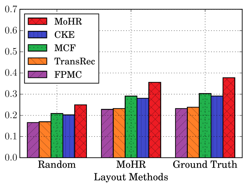
(a) Automotive

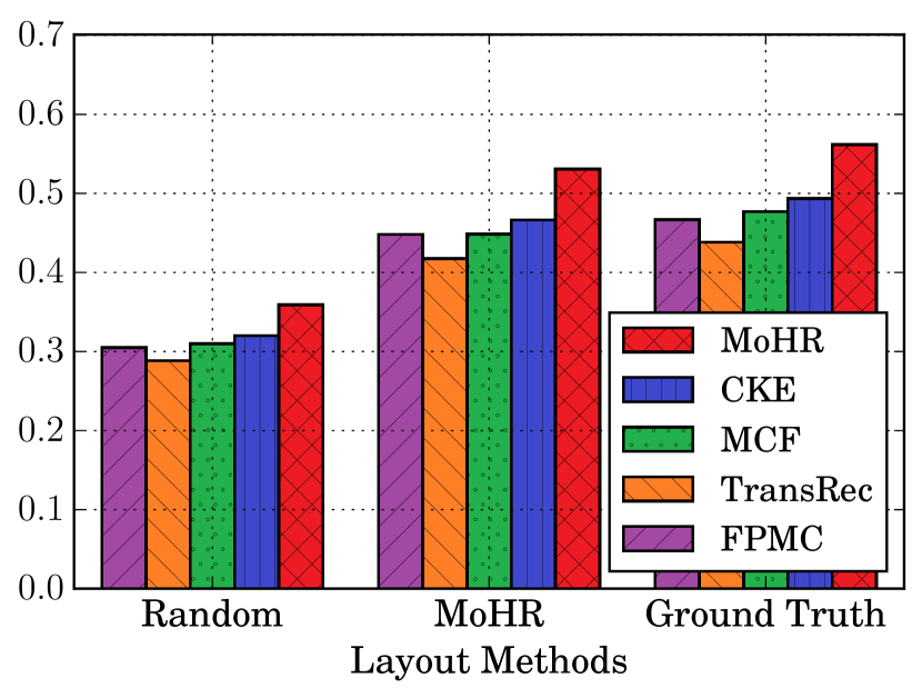
(b) Games

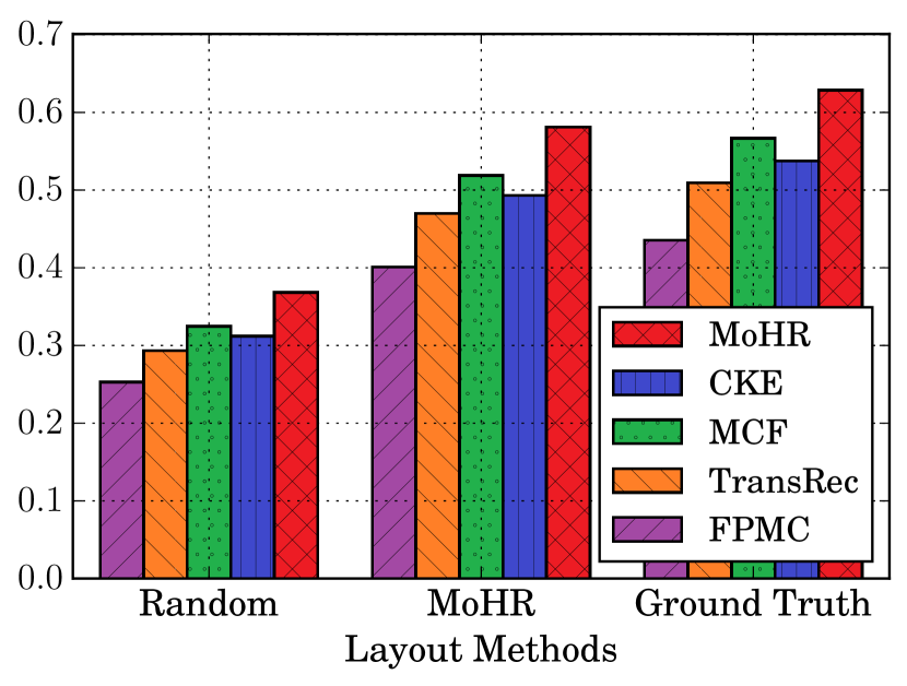
(c) Google

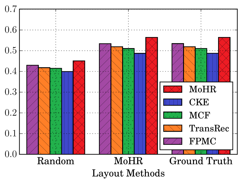
(d) Steam

Figure 3. Ranking performance (NDCG) under Setting-2 with different layout methods.

4.2. Comparison Methods

To show the effectiveness of MoHR, we include three groups of recommendation methods. The first group includes general recommendation methods which only consider user feedback without considering the sequence order of actions:

• PopRec: This is a simple baseline that ranks items according to their popularity (i.e., number of associated actions).

• Bayesian Personalized Ranking (BPR-MF) (Rendle et al., 2009): BPR-MF is a classic method of learning personalized ranking from implicit feedback. Biased matrix factorization is used as the underlying recommender.

• Collaborative Metric Learning (CML) (Hsieh et al., 2017): A state-of-the-art collaborative filtering method that learns metric embeddings for users and items.

The second group contains sequential recommendation methods, which consider the sequence of user actions:

• Factorized Personalized Markov Chains (FPMC) (Rendle et al., 2010): FPMC uses a combination of matrix factorization and factorized Markov chains as its recommender, which captures users’ long-term preferences as well as item-to-item transitions.

• Translation-based Recommendation (TransRec) (He et al., 2017a): A state-of-the-art sequential recommendation method which models each user as a translation vector to capture the transition from the current item to the next item.

The final group of methods uses item relationships as regularizers:

• Preference and Context Embedding (PACE) (Yang et al., 2017): A neural POI recommendation method that learns user and item embeddings with regularization by preserving user-to-user and item-to-item neighborhood structure.

• Matrix Co-Factorization (MCF) (Park et al., 2017): A recent method which showed that “also viewed” data helps rating prediction. It simultaneously factorizes a rating matrix and a binary item-to-item matrix based on “also viewed” products.

• Collaborative Knowledge base Embedding (CKE) (Zhang et al., 2016): A collaborative filtering method with regularizations from visual, textual and structural item information.

Finally, our own method, Mixtures of Heterogeneous Recommenders (MoHR), makes use of various recommenders to capture both long-term preferences and (explicit/latent) item transitions in a unified translational metric space.

A summary of methods above is shown in Table 2. For fair comparison, we implement all methods in TemsorFlow with the Adam (Kingma and Ba, 2014) optimizer. All learning-based methods use BPR or S-BPR loss functions to optimize personalized rankings. For PACE, MCF, and CKE, we do not use side information other than item relationships. For methods with homogeneous item similarities (i.e., PACE and MCF), we define two items as ‘neighbors’ if they share at least one relationship. For CKE, we use TransE (Bordes et al., 2013) to model item relationships. Regularization hyper-parameters are selected from {0,0.0001,0.001,0.01,0.1} using our validation set. Our method can achieve satisfactory performance using $\alpha=1$, $\beta=0.1$ and $\lambda=1e\text{-}4$ for all datasets except Steam. Due to its high density, we use $\alpha=0.1$, $\beta=0.1$ and $\lambda=0$ for Steam. More detailed hyper-parameter analysis is included in Section 4.5.

4.3. Evaluation Metrics

Setting-1. The first is a typical sequential recommendation setting which recommends items given a user $u$ and her last visited item $i$. Here the ground-truth next item should be ranked as high as possible. In this setting, we report the AUC, Hit Rate@10, and NDCG@10 as in (He et al., 2017a; Yang et al., 2017; Tay et al., 2018). The AUC measures the overall ranking performance whereas HR@10 and NDCG@10 measure Top-N recommendation performance. HR@10 simply counts whether the ground-truth item is ranked among the top-10 items, while NDCG@10 is a position-aware ranking metric.

For top-n ranking performance metrics, to avoid heavy computation on all user-item pairs, we followed the strategy in (Koren, 2008; Tay et al., 2018; He et al., 2017b). For each user $u$, we randomly sample 100 irrelevant items (i.e., doesn’t belong to $\mathcal{S}^{u}$), and rank these items with the ground-truth item. Based on rankings of these 101 items, HR@10 and NDCG@10 can be evaluated.

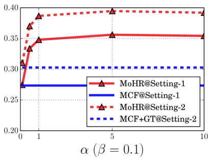
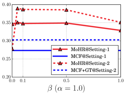
(a) Automotive

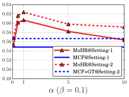
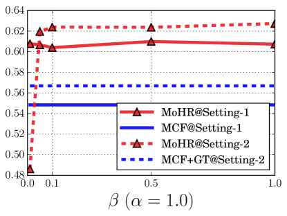
(b) Google

Figure 4. Effect of Hyper-parameter $\alpha$ and $\beta$. Ranking performance regarding NDCG@10 and NDCG under two settings is shown in the figure respectively. The blue line indicates the strongest baseline in the corresponding dataset.

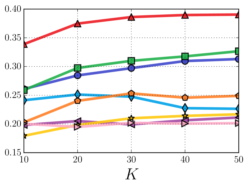
(a) Automotive

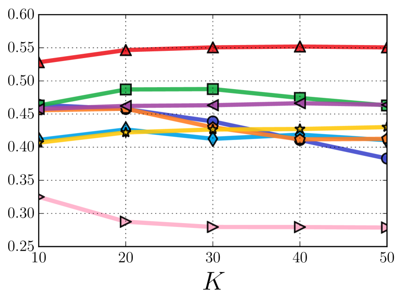
(b) Video Games

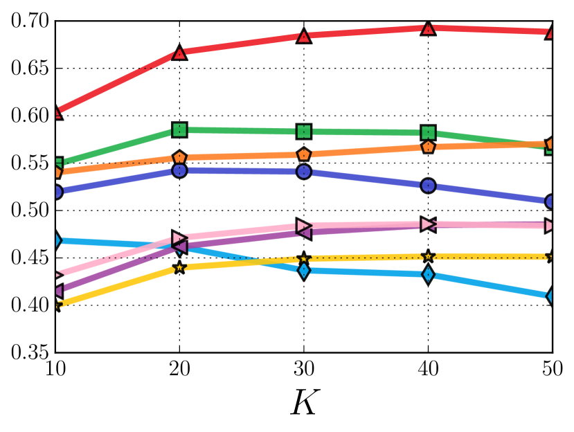
(c) Google

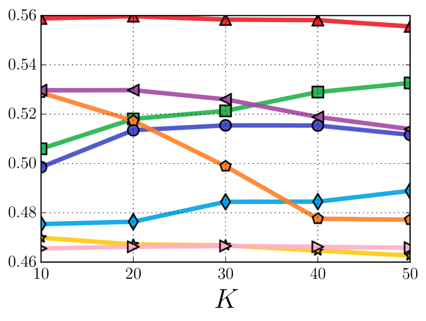
(d) Steam

Figure 5. Effect of Hyper-parameter $K$. Ranking performance regarding NDCG@10 under Setting-1 is shown in the figure.

Setting-2. In the second setting, we consider a practical recommendation scenario that shows recommendations type by type (e.g. like the interface in Figure 1 and our example in Figure 6). There are two objectives: 1) relevant relationships (i.e., contains relevant items) should be highly ranked; and 2) within each relationship, relevant items should be highly ranked. Specifically, for a given user and her last visited item, we first rank relationships, then we display at most 10 items from each relationship. Therefore, the ultimate position of an item $i$ is decided by its ranking within the relationship as well as the ranking of the relationship to which $i$ belongs. We use NDCG to evaluate the ranking performance, which considers the positions of relevant items.

4.4. Recommendation Performance

Table 4 shows results under the typical sequential recommendation setting. The number of latent dimensions $K$ is set to 10 for all experiments. Results on larger $K$ are analyzed in section 4.5.

We find our method MoHR can outperform all baselines on all datasets in terms of both overall ranking and top-n ranking metrics. Compared to sequential feedback based methods (FPMC and TransRec), the results show the important role of item-to-item relationships on understanding users’ sequential behavior. Compared to methods that rely on item relationships as regularization (PACE, MCF and CKE), the performance of our method shows the advantages of modeling item relationships and sequential signals jointly. Another observation is sequential methods FPMC and TransRec achieve better performance than relationship-ware methods on Steam, presumably due to the high density of sequential feedback (beneficial for learning latent transitions) and sparsity of related items (insufficient for capturing item similarities) in Steam.

For Setting-2, a recommendation method should decide the order in which to show relationships as well as the rank of items from each relationship. All methods are capable of ranking items for different users. However, only our method MoHR models the next-relationship problem and can give a prediction of relationship ranking. Figure 3 shows the results of our method and four strong baselines under three relationship ranking methods: random, MoHR’s relationship ranking prediction (i.e., $P(r|u,i)$) and the ground-truth relationship ranking (i.e., relationships that contain ground-truth items are ranked higher than others). We can see MoHR can outperform the baselines under all three relationship ranking methods, and MoHR (with its own relationship ranking) can beat baselines with the ground-truth ranking. This shows the effectiveness of our method on both relationship and item ranking.

4.5. Effect of Hyper-parameters

We empirically analyze the effect of the hyper-parameters in our model. Figure 4 shows the influence of $\alpha$, $\beta$ under the two settings. When $\alpha\to 0$, item vectors ${\bm{\theta}}_{i}$ and relationship vectors ${\bm{\theta}}_{r}$ are free to fit sequential feedback without the constraint from relationships. As $\alpha$ increases, the performance on both settings improves and then degrades, which is similar to the effect of regularization. $\beta$ (the hyper-parameter controlling the prior of choosing the next relationship) doesn’t improve the performance significantly on Setting-1. However, when $\beta\to 0$, the model is not aware of how users choose their next relationship, which leads to poor performance on Setting-2, due to poor relationship ranking. Typically when $\alpha=1$ and $\beta=0.1$, the model can achieve satisfactory performance on both settings. For the latent dimensionality $K$, Figure 5 shows the recommendation performance of all the baselines with K varying from $10$ to $50$. We can find that our method outperforms baselines across the full spectrum of values.

4.6. Ablation Study

We analyze the effect of each component in MoHR by ablation study. First, recall that MoHR’s predictor $R^{*}$ (in eq. (6)) contains two terms for long-term preference and mixture of short-term transitions (respectively). If the second term (for the mixture) is removed, then the predictor is equivalent to TransRec’s. Hence we analyze the effect of the mixture term by comparing the performance of using/not using the mixture. Second, our optimization problem contains two auxiliary tasks ($T_{I}$ and $T_{R}$ in eq. (8)). Without the two tasks, our model is not able to utilize explicit item relationships. By enumerating all the options, we induce four variants in total, and their recommendation performance (NDCG@10) is shown in Table 5.

We can see that multi task learning can significantly boost the performance on all datasets, implying the importance of using explicit item transitions for next item recommendation. Also, using the mixture of short-term transitions consistently improves performance when multi task learning is employed. For single task cases where all transitions are latent, using the mixture can boost performance on all datasets except Google. Overall, the full model of MoHR (multi task+mixture) achieves the best performance.

Table 5. Performance using different components of MoHR

Component	Auto	Video	Google	Steam
Single Task	0.1805	0.4617	0.4371	0.5276
Single Task + Mixture	0.1864	0.4626	0.4069	0.5360
Multi Tasks	0.3304	0.5214	0.6002	0.5588
Multi Tasks + Mixture	0.3478	0.5366	0.6091	0.5598

4.7. Comparison to Deep Learning Approaches

We also compare our methods against deep learning based methods that seek to capture sequential patterns for recommendation. Specifically, two baselines are : 1) GRU4Rec (Hidasi et al., 2016) is a seminal method that uses RNNs for session-based recommendation. For comparison we treat each user’s feedback sequence as a session; 2) GRU4Rec (revised) (Hidasi and Karatzoglou, 2017) is an improved version which adopts a different loss function and sampling strategy; 3) Convolutional Sequence Embedding (Caser) (Tang and Wang, 2018) is a recent method for sequential recommendation, which treats embeddings of preceding items as an ‘image’ and extracts sequential features by applying convolutional operations. We use the code from the corresponding authors, and conduct experiments on a workstation with a single GTX 1080 Ti GPU.

Table 6 shows the Top-N ranking performance (NDCG@10) of baselines and our method MoHR on four datasets. MoHR outperforms all baselines significantly on all datasets except Steam. GRU4Rec (revised) shows the best performance on Steam, while MoHR is slightly worse. Presumably this is because Steam is a relatively dense dataset, where CNN/RNN-based methods can learn higher order sequential patterns while MoHR only considers the last visited item. We can also see the gap between Caser and MoHR on Steam is smaller than that on other datasets, which could also be attributed to density. Though deep learning based methods are computationally expensive and don’t tend to perform well on sparse datasets, in the future we hope to incorporate them into MoHR to capture higher-order item transitions while alleviating data scarcity problems by considering explicit item relationships.

Table 6. Comparison to CNN/RNN-based Methods

Method	Auto	Video	Google	Steam
GRU4Rec (original) (Hidasi et al., 2016)	0.0848	0.2250	0.4166	0.3521
GRU4Rec (revised) (Hidasi and Karatzoglou, 2017)	0.1246	0.3132	0.4032	0.5676
Caser (Tang and Wang, 2018)	0.2518	0.3075	0.2244	0.5141
MoHR	0.3478	0.5366	0.6091	0.5598

4.8. Qualitative Examples

Figure 6 illustrates a practical recommendation scenario using our method MoHR on the Amazon Automotive dataset. We can see that MoHR can generate a layout and recommendations according to the context $(u,i)$. This may also provide a way to interpret users’ intentions behind their behavior. For example, User A in the figure may want to try another brand of oil whereas User B may seek complementary accessories.

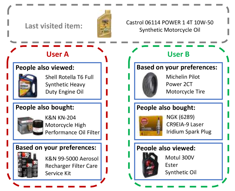
Figure 6. A recommendation example for two users with the same last visited item. For each type of recommendation, we display the top result. The order of relationships is decided by $P(r|u,i)$. This shows how our model generates different layouts according to user context.

Recall that we use $r_{0}$ to capture latent transitions (unexplained by explicit relationships) from sequential feedback. To show the latent transitions learned by transition vector ${\bm{\theta}}_{r_{0}}$, We train a model without bias terms (for better illustration) on Google Local. Table 7 shows consecutive transitions starting from various popular POIs. Unlike explicit relationships which only represent “nearby businesses” and “similar businesses,” the latent relationship can capture richer semantics and long-range transitions from sequential feedback.

Table 7. Transition examples using the latent relationship $r_{0}$. Place $i$’s next place is the nearest neighbor of ${\bm{\theta}}_{i}+{\bm{\theta}}_{r_{0}}$. We can see $r_{0}$ is able to capture meaningful transitions with various semantics and ranges.

Universal Studios Hollywood $\rightarrow$ Hollywood Sign $\rightarrow$ LAX Airport

Universal Studios Orlando $\rightarrow$ Disney World Resort $\rightarrow$ Florida Mall

Universal Studios Japan $\rightarrow$ Yodobashi Akiba $\rightarrow$ Edo-Tokyo Museum

JFK Airport (New York) $\rightarrow$ Statue of Liberty $\rightarrow$ Empire State Building

Heathrow Airport (London)$\rightarrow$ London Bridge $\rightarrow$ Croke Park (Ireland)

Hong Kong Airport $\rightarrow$ The Peninsula Hong Kong $\rightarrow$ Hong Kong Park

Death Valley National Park $\rightarrow$ Circus Circus (Las Vegas) $\rightarrow$ Yellowstone

Louvre Museum $\rightarrow$ Eiffel Tower $\rightarrow$ Charles de Gaulle Airport (Paris)

5. Conclusion

In this work we present a sequential recommendation method MoHR, which learns a personalized mixture of heterogeneous (explicit/latent) item-to-item recommenders. We represent all parameters in a unified metric space and adopt translational operations to model their interactions. Multi-task learning is employed to jointly learn the embeddings across the three tasks. Extensive quantitative results on large-scale datasets from various real-world applications demonstrate the superiority of our method regarding both overall and Top-N recommendation performance.

References

- (1)
- Beutel et al. (2018) Alex Beutel, Paul Covington, Sagar Jain, Can Xu, Jia Li, Vince Gatto, and Ed H Chi. 2018. Latent Cross: Making Use of Context in Recurrent Recommender Systems. In WSDM’18.
- Bordes et al. (2013) Antoine Bordes, Nicolas Usunier, Alberto Garcia-Duran, Jason Weston, and Oksana Yakhnenko. 2013. Translating embeddings for modeling multi-relational data. In NIPS’13.
- Caruana (1997) Rich Caruana. 1997. Multitask Learning. Machine Learning (1997).
- Chen et al. (2012) Shuo Chen, Josh L Moore, Douglas Turnbull, and Thorsten Joachims. 2012. Playlist prediction via metric embedding. In KDD’12.
- Feng et al. (2015) Shanshan Feng, Xutao Li, Yifeng Zeng, Gao Cong, Yeow Meng Chee, and Quan Yuan. 2015. Personalized ranking metric embedding for next new POI recommendation. In IJCAI’15.
- Garcia-Duran et al. (2018) Alberto Garcia-Duran, Roberto Gonzalez, Daniel Onoro-Rubio, Mathias Niepert, and Hui Li. 2018. TransRev: Modeling Reviews as Translations from Users to Items. arXiv preprint arXiv:1801.10095 (2018).
- He et al. (2017a) Ruining He, Wang-Cheng Kang, and Julian McAuley. 2017a. Translation-based Recommendation. In RecSys’17.
- He and McAuley (2016) Ruining He and Julian McAuley. 2016. Fusing similarity models with markov chains for sparse sequential recommendation. In ICDM’16.
- He et al. (2017b) Xiangnan He, Lizi Liao, Hanwang Zhang, Liqiang Nie, Xia Hu, and Tat-Seng Chua. 2017b. Neural collaborative filtering. In WWW’17.
- Hidasi and Karatzoglou (2017) Balázs Hidasi and Alexandros Karatzoglou. 2017. Recurrent Neural Networks with Top-k Gains for Session-based Recommendations. arXiv abs/1706.03847 (2017).
- Hidasi et al. (2016) Balázs Hidasi, Alexandros Karatzoglou, Linas Baltrunas, and Domonkos Tikk. 2016. Session-based Recommendations with Recurrent Neural Networks. In ICLR’16.
- Hsieh et al. (2017) Cheng-Kang Hsieh, Longqi Yang, Yin Cui, Tsung-Yi Lin, Serge J. Belongie, and Deborah Estrin. 2017. Collaborative Metric Learning. In WWW’17.
- Hu et al. (2008) Yifan Hu, Yehuda Koren, and Chris Volinsky. 2008. Collaborative filtering for implicit feedback datasets. In ICDM’08.
- Jacobs et al. (1991) Robert Jacobs, Michael Jordan, Steven Nowlan, and Geoffrey Hinton. 1991. Adaptive Mixtures of Local Experts. Neural Computation (1991).
- Jing and Smola (2017) How Jing and Alexander J. Smola. 2017. Neural Survival Recommender. In WSDM’17.
- Kabbur et al. (2013) Santosh Kabbur, Xia Ning, and George Karypis. 2013. FISM: factored item similarity models for top-n recommender systems. In KDD’13.
- Kang et al. (2017) Wang-Cheng Kang, Chen Fang, Zhaowen Wang, and Julian McAuley. 2017. Visually-Aware Fashion Recommendation and Design with Generative Image Models. In ICDM’17.
- Kim et al. (2016) Dong Hyun Kim, Chanyoung Park, Jinoh Oh, Sungyoung Lee, and Hwanjo Yu. 2016. Convolutional Matrix Factorization for Document Context-Aware Recommendation. In RecSys’16.
- Kingma and Ba (2014) Diederik P Kingma and Jimmy Ba. 2014. Adam: A method for stochastic optimization. arXiv preprint arXiv:1412.6980 (2014).
- Koren (2008) Yehuda Koren. 2008. Factorization meets the neighborhood: a multifaceted collaborative filtering model. In KDD’08.
- Koren (2010) Yehuda Koren. 2010. Collaborative filtering with temporal dynamics. Commun. ACM (2010).
- Koren et al. (2009) Yehuda Koren, Robert Bell, and Chris Volinsky. 2009. Matrix Factorization techniques for recommender systems. Computer (2009).
- Li et al. (2017) Jing Li, Pengjie Ren, Zhumin Chen, Zhaochun Ren, Tao Lian, and Jun Ma. 2017. Neural Attentive Session-based Recommendation. In CIKM’17.
- Lin et al. (2015) Yankai Lin, Zhiyuan Liu, Maosong Sun, Yang Liu, and Xuan Zhu. 2015. Learning Entity and Relation Embeddings for Knowledge Graph Completion. In AAAI’15.
- Liu et al. (2013) Bin Liu, Yanjie Fu, Zijun Yao, and Hui Xiong. 2013. Learning geographical preferences for point-of-interest recommendation. In KDD’13.
- McAuley et al. (2015a) Julian McAuley, Rahul Pandey, and Jure Leskovec. 2015a. Inferring networks of substitutable and complementary products. In KDD’15.
- McAuley et al. (2015b) Julian McAuley, Christopher Targett, Qinfeng Shi, and Anton van den Hengel. 2015b. Image-based recommendations on styles and substitutes. In SIGIR’15.
- Park et al. (2017) Chanyoung Park, Dong Hyun Kim, Jinoh Oh, and Hwanjo Yu. 2017. Do ”Also-Viewed” Products Help User Rating Prediction?. In WWW’17.
- Pathak et al. (2017) Apurva Pathak, Kshitiz Gupta, and Julian McAuley. 2017. Generating and Personalizing Bundle Recommendations on Steam. In SIGIR’17.
- Pei et al. (2017) Wenjie Pei, Jie Yang, Zhu Sun, Jie Zhang, Alessandro Bozzon, and David MJ Tax. 2017. Interacting Attention-gated Recurrent Networks for Recommendation. In CIKM’17.
- Rendle et al. (2009) Steffen Rendle, Christoph Freudenthaler, Zeno Gantner, and Lars Schmidt-Thieme. 2009. BPR: Bayesian personalized ranking from implicit feedback. In UAI’09.
- Rendle et al. (2010) Steffen Rendle, Christoph Freudenthaler, and Lars Schmidt-Thieme. 2010. Factorizing personalized markov chains for next-basket recommendation. In WWW’10.
- Sedhain et al. (2015) Suvash Sedhain, Aditya Krishna Menon, Scott Sanner, and Lexing Xie. 2015. Autorec: Autoencoders meet collaborative filtering. In WWW’15.
- Shu et al. (2018) Kai Shu, Suhang Wang, Jiliang Tang, Yilin Wang, and Huan Liu. 2018. Crossfire: Cross media joint friend and item recommendations. In WSDM’18.
- Smirnova and Vasile (2017) Elena Smirnova and Flavian Vasile. 2017. Contextual Sequence Modeling for Recommendation with Recurrent Neural Networks. In DLRS@RecSys’17.
- Tang and Wang (2018) Jiaxi Tang and Ke Wang. 2018. Personalized Top-N Sequential Recommendation via Convolutional Sequence Embedding. In WSDM’18.
- Tay et al. (2018) Yi Tay, Luu Anh Tuan, and Siu Cheung Hui. 2018. Latent Relational Metric Learning via Memory-based A ention for Collaborative Ranking. In WWW’18.
- Tuan and Phuong (2017) Trinh Xuan Tuan and Tu Minh Phuong. 2017. 3D Convolutional Networks for Session-based Recommendation with Content Features. In RecSys’17.
- Wang et al. (2015) Hao Wang, Naiyan Wang, and Dit-Yan Yeung. 2015. Collaborative Deep Learning for Recommender Systems. In KDD’15.
- Wang et al. (2017) Suhang Wang, Yilin Wang, Jiliang Tang, Kai Shu, Suhas Ranganath, and Huan Liu. 2017. What your images reveal: Exploiting visual contents for point-of-interest recommendation. In WWW’17.
- Wu et al. (2017) Le Wu, Yong Ge, Qi Liu, Enhong Chen, Richang Hong, Junping Du, and Meng Wang. 2017. Modeling the evolution of users’ preferences and social links in social networking services. IEEE TKDE (2017).
- Yang et al. (2017) Carl Yang, Lanxiao Bai, Chao Zhang, Quan Yuan, and Jiawei Han. 2017. Bridging Collaborative Filtering and Semi-Supervised Learning: A Neural Approach for POI Recommendation. In KDD’17.
- Yi et al. (2014) Xing Yi, Liangjie Hong, Erheng Zhong, Nanthan Nan Liu, and Suju Rajan. 2014. Beyond clicks: dwell time for personalization. In RecSys’14.
- Yu et al. (2014) Xiao Yu, Xiang Ren, Yizhou Sun, Quanquan Gu, Bradley Sturt, Urvashi Khandelwal, Brandon Norick, and Jiawei Han. 2014. Personalized entity recommendation: A heterogeneous information network approach. In WSDM’14.
- Zhang et al. (2016) Fuzheng Zhang, Nicholas Jing Yuan, Defu Lian, Xing Xie, and Wei-Ying Ma. 2016. Collaborative Knowledge Base Embedding for Recommender Systems. In KDD’16.
- Zhang et al. (2017) Shuai Zhang, Lina Yao, and Aixin Sun. 2017. Deep Learning based Recommender System: A Survey and New Perspectives. arXiv abs/1707.07435 (2017).
- Zhao et al. (2017) Huan Zhao, Quanming Yao, Jianda Li, Yangqiu Song, and Dik Lun Lee. 2017. Meta-graph based recommendation fusion over heterogeneous information networks. In KDD’17.
- Zhao et al. (2014) Tong Zhao, Julian McAuley, and Irwin King. 2014. Leveraging social connections to improve personalized ranking for collaborative filtering. In CIKM’14.