October 30, 2018

$*$Corresponding author
^† E-mail: chan@arrhenius.med.utoronto.ca; Tel: (416)978-2697; Fax: (416)978-8548
^† Mailing address:
^† Department of Biochemistry, University of Toronto, Medical Sciences Building – 5th Fl.,
^† 1 King’s College Circle, Toronto, Ontario M5S 1A8, Canada.

Abstract

Biomolecular condensates undergirded by phase separations of proteins and nucleic acids serve crucial biological functions. To gain physical insights into their genetic basis, we study how liquid-liquid phase separation (LLPS) of intrinsically disordered proteins (IDPs) depends on their sequence charge patterns using a continuum Langevin chain model wherein each amino acid residue is represented by a single bead. Charge patterns are characterized by the “blockiness” measure $\kappa$ and the “sequence charge decoration” (SCD) parameter. Consistent with random phase approximation (RPA) theory and lattice simulations, LLPS propensity as characterized by critical temperature $T^{*}_{\rm cr}$ increases with increasingly negative SCD for a set of sequences showing a positive correlation between $\kappa$ and $-$SCD. Relative to RPA, the simulated sequence-dependent variation in $T^{*}_{\rm cr}$ is often—though not always—smaller, whereas the simulated critical volume fractions are higher. However, for a set of sequences exhibiting an anti-correlation between $\kappa$ and $-$SCD, the simulated $T^{*}_{\rm cr}$’s are quite insensitive to either parameters. Additionally, we find that blocky sequences that allow for strong electrostatic repulsion can lead to coexistence curves with upward concavity as stipulated by RPA, but the LLPS propensity of a strictly alternating charge sequence was likely overestimated by RPA and lattice models because interchain stabilization of this sequence requires spatial alignments that are difficult to achieve in real space. These results help delineate the utility and limitations of the charge pattern parameters and of RPA, pointing to further efforts necessary for rationalizing the newly observed subtleties.

1 Introduction

Functional biomolecular condensates of proteins and nucleic acids—some of which are referred to as membraneless organelles—have been garnering intense interest since the recent discoveries of liquid-like behaviors of germline P-granules in Caenorhabditis elegans brangwynne2009 and observations of phase transitions from solution to condensed liquid and/or to gel states in cell-free systems containing proteins with significant conformational disorder.Rosen12 ; McKnight12 ; Nott15 ; tanja2015 ; parker2015 In hindsight, the possibility that certain cellular compartments were condensed liquid droplets has already been raised more than a century ago when the protoplasm of echinoderm (e.g. star-fish and sea-urchin) eggs was seen as an emulsion with granules or microsomes as its basic components.wilson1899 Subsequently, in two studies nearly half a century apart, the nucleolus was hypothesized to be a “coacervate”, a “separated phase out of a saturated solution” lars1946 and, more generally, phase separation in the cytoplasm was proposed to be “the basis for microcompartmentation”.brooks1995 Now, burgeoning investigative efforts on biomolecular condensates in the past few years have yielded many advances (refsrosen2017 ; cliff2017 ; eggert2018 ; dinneny2018 and references therein). To name a few, phase separations of intrinsically disordered proteins (IDPs) or folded protein domains connected by disordered linkers are critical in the formation and organization of the nucleolus Feric16 (as anticipated seventy years earlier lars1946 ), the nuclear pore complex anton ; anton_biochem , postsynaptic densities MJZ2016 ; MJZbiochem , P-granules Nott15 , and stress granules.tanja2015 ; Riback_etal2017 They are also responsible for the ability of tardigrades (“water bears”) to survive desiccation boothby2017 and the synthesis of squid beaks squid as well as byssuses for anchoring mussels onto sea rocks.mussel More speculatively, the compartmentalization afforded by IDP phase separation might even be important in the origin of life keating1 ; keating2 as envisioned in the Oparin theory oparin and its modern derivatives.dysonJ ; dysonB Because of the crucial roles of biomolecular condensates in physiological functions, their dysfunction can lead to diseases such as pathological protein fibrillization tanja2015 and neurological disorders.MJZ2016

Properties of IDPs and their phase separations are dependent, as physically expected, upon the amino acid sequences of the IDPs.Nott15 ; muthu-pattern ; pappu13 ; PappuCOSB However, deciphering genetically encoded sequence effects on biologically functional biomolecular condensates is difficult in general because the interactions within such condensates can be extremely complex, often involving many species of proteins and nucleic acids and the condensates are sometimes maintained by non-equilibrium processes.cliff2017 ; Deniz17 ; babu2018 ; pappu2018 For instance, some crucial interactions in biomolecular condensates can be ATP-modulated as in stress granules ATP1 , others can be tuned by post-translational modifications as exemplified by phosphorylations of Fused in Sarcoma (FUS).fus1 ; fus2 Biomolecular condensates are “active liquids” in this regard.active2011 ; active2017 ; berry2018 ; lee2018 Moreover, some biomolecular condensates are not entirely liquid-like but rather exhibit gel- or solid-like characters.gelation ; biochemrev By comparison, experimental biophysical studies often focus, for tractability, on equilibrium properties of simple condensates consisting of only a few biomolecular components. Nonetheless, although these constructs are highly simplified models of in vivo biomolecular condensates, knowledge gained from their study is extremely useful not only as a scientific stepping stone to understanding the workings of complex in vivo biomolecular condensates but also as an engineering tool for designing bioinspired materials.steph17 ; chilkoti2015 ; singperry2017 ; chilkoti2017 ; rohitJMB

Currently, theoretical approaches to sequence-dependent biophysical properties of biomolecular condensates are only in their initial stages of development. These efforts—which include analytical theories and explicit-chain simulations—have been focusing on general principles and rationalization of experimental data on simple systems. Analytical theories are an efficient investigative tool despite their limited, approximate treatment of structural and energetic details.biochemrev For example, predictions of mean-field Flory-Huggins (FH)-type theories Nott15 ; CellBiol ; NatPhys are sensitive to IDP amino acid compositions but FH theories do not distinguish different IDP sequences sharing the same composition. Nevertheless, such theories can be very useful, as demonstrated by a recent formulation that rationalizes how FUS phase behaviors depend on tyrosine and arginine compositions.moleculargrammar By comparison, more energetic details of multiple-chain IDP interactions are captured by random phase approximation (RPA), which is an analytical formulation delaCruz2003 that offers a rudimentary account of sequence-dependent electrostatic effects on IDP phase behaviors.linPRL ; linJML ; lin2017 ; njp2017 Because it allows for the treatment of any arbitrary sequence of charges, RPA has proven useful in accounting for the experimental effects of sequence charge pattern on the phase properties of RNA helicase Ddx4 (refsNott15 ; linPRL ). It is also instrumental in proposing a novel correlation between sequence-dependent single-chain properties and multiple-chain phase behaviors lin2017 —which was recently verified by explicit-chain simulations jeetainPNAS —and in suggesting a new form of “fuzzy” molecular recognition based on charge pattern matching.njp2017 In this connection, another recent approach that combines transfer matrix theory and simulation has also been useful in accounting for complex coacervation involving polypeptides with simple repeating sequence charge patterns.singperry2017 ; lytle2017 Building on these advances, further work will be needed to develop theories that can account for sequence-dependent non-electrostatic effects, including hydrophobicity, cation-$\pi$ interactions—which play significant roles in functional larry2014 and disease-causing kaw2013 IDP interactions and in the formation of biomolecular condensates Nott15 ; mussel —as well as aromatic diederich and non-aromatic robert $\pi$–$\pi$ interactions which are likely of importance in the assembly of biomolecular condensates.robert

Explicit-chain models and analytical theories are complementary. Compared to analytical theories, explicit-chain simulations of IDP phase separation are computationally expensive because they require tracking the configurations of a multiple-chain model system that is sufficiently large to represent phase-separated states. Yet explicit-chain simulations are necessary for a realistic representation of chain geometry and thus indispensable also for evaluating the approximations invoked by analytical theories.suman1 ; suman1C Phase separation of IDP and/or folded protein domains connected by disordered linkers have been simulated using highly coarse-grained models consisting of basic units each designed to represent groups of amino acid residues.gelation ; Ruff15 ; harmonNJP These constructs have yielded physical insights into the phase behaviors of a four-component system,harmonNJP for example. Also utilized recently for explicit-chain modeling of biomolecular condensates are coarse-grained approaches that capture more structural and energetic details by representing each amino acid residue of an IDP as a single bead on a chain.jeetainPNAS ; suman1 ; dignon18 Because we are interested in biomolecular condensates in which the protein chains are significantly disordered,fawzi2015 ; jacob2017 analytical theories foffi2009 ; vojko2015 ; vojko2016 and simulation techniques foffi2007 ; foffi2011 ; hxzhou2018 developed for the phase separation of folded proteins hxzhou2016 ; hxzhou2017 (e.g. $\gamma$-crystallin crystallin and lysozyme lysozyme ; lysozymeP ) are not directly applicable. Our group has previously employed lattice models to study sequence-dependent electrostatic effects on IDP phase separation.suman1 To assess the extent to which predictions from these models are affected by lattice artifacts and to broaden our effort to model biomolecular condensates in general, here we apply more realistic coarse-grained models wherein IDP chains are configured in the continuum.JChen2012 ; cosb15 ; Best2017 ; Shea2017

Coarse-grained explicit-chain models are well-suited to address general physical principles. The rapidly expanding experimental efforts have provided an increasing rich set of data on overall physical properties of biomolecular condensates that awaits theoretical analysis. For instance, although solutions with temperature-independent effective solute-solute interactions are expected to phase separate when temperature is reduced below a certain upper critical solution temperature (UCST)—in which case phase separation propensity at a given temperature increases with increasing critical temperature $T^{*}_{\rm cr}=$ UCST, some biomolecular condensates are formed at raised temperatures (i.e., they possess a lower critical solution temperature, LCST)—in which case phase separation propensity at a given temperature decreases with increasing $T^{*}_{\rm cr}=$ LCST. Examples of the latter include elastin,elastin1 ; lisa ; tanja2018 the Alzheimer-disease-related tau protein,tau and the Poly(A)-binding protein Pab1 associated with stress granules in yeast.Riback_etal2017 Recent experiments on elastin indicate that formation of biomolecular condensates can also be dependent upon hydrostatic pressure.roland18 As has been suggested,biochemrev ; roland18 these phenomena may be accounted for, at least semi-quantitatively, by temperature maria and pressure cristiano ; heinrich -dependent sidechain alex2018 and backbone IDP interactions.biochemrev

Building on our recent lattice simulation,suman1 we focus here on sequence-dependent electrostatic effects on IDP phase separation. Previous studies by analytical theories lin2017 ; njp2017 and explicit-chain lattice simulations suman1 of IDPs with different charge patterns suggest that their propensities to phase separate are well correlated with two parameters for characterizing sequence charge pattern: the intuitive $\kappa$ parameter for “blockiness” of the charge arrangement along a sequence pappu13 ; PappuCOSB and the “sequence charge decoration” SCD parameter that arose from a theory for the conformational dimensions of polyampholytes.Sawle15 ; Sawle17 ; Firman18 If such parameters (and even simpler properties such as the net charge of a sequence) can predict certain aspects of IDP phase separation, they may shed light on the relevant “holistic” physical properties underpinning certain shared biological functions among IDP sequences that are otherwise highly diverse on a residue-by-residue basis.moses17 ; doug2017 These parameters could be useful for designing artificial protein polymers as well.chilkoti2018 Remarkably, although both $\kappa$ and SCD originated from studies of single-chain IDP properties, they appear to capture also the propensities of multiple IDP chains to phase separate.lin2017 ; njp2017 ; suman1 In view of the prospective broad utility of this putative relationship, its generality deserves closer scrutiny.

2 Scope and rationale

With the above consideration in mind, the present study compares polyampholytes phase properties predicted by RPA theory against those simulated by explicit-chain models, and assesses the ability of $\kappa$ and SCD to capture the theoretical/simulated trends. The interplay between the effects of charge-dependent electrostatic and charge-independent Lennard-Jones-type interactions on polyampholyte phase behaviors is also explored.

Insofar as explicit-chain modeling of biomolecular systems is concerned, atomic models with detailed structural and energetic representations and coarse-grained models are complementary when both approaches are viable for the system in question. Despite their relative lack of structural and energetic details—and in some cases precisely because of this lack of details—coarse-grained models have contributed significantly to theoretical advances since they are computationally efficient tools for conceptual development and for discovery of universality across a large class of seemingly unrelated phenomena. For instance, early exact enumerations of conformational statistics of lattice polymers domb69 was instrumental in the subsequent fundamental development of scaling deGennes79 and renormalization group freed1987 theories in polymer physics. Other examples include lattice investigations of protein folding kinetics kaya03 and DNA topology Liu06 that led to more sophisticated models confirming insights originally gained from earlier lattice studies.TaoPCCP ; Liu15 Lattice models are a powerful tool for the study of homopolymer phase separation as well,panagio1998 although their applicability to long heteropolymeric chains might be limitedpanagio2003 ; panagio2005 as has been noted.suman1 Moving beyond the confines of lattices, here we consider model chains configured in continuum space.

The determination of phase diagrams of IDP liquid-liquid phase separation (LLPS) is computationally intensive. Currently, all-atom explicit-water molecular dynamics is not feasible for this task. Even a recent state-of-the-art molecular dynamics study of the liquid structure of elastin that clocked a total simulated time of 165 $\mu$s could only model a droplet of twenty seven 35-residue elastin-like peptides and did not provide a phase diagram.regis17 Besides issues of computational efficiency, common molecular dynamics force fields are well known to be problematic for IDPs.DavidShaw2 ; sarah15 Developing a force field that is suitable for both IDPs and globular proteins has been a major ongoing challenge.best14 ; sarah17 ; Shaw18

In this context, we adapt the coarse-grained model of Dignon et al.,jeetainPNAS ; dignon18 which in turn is partly based upon simulation algorithms developed for vapor-liquid transitions.blas2008 ; panag2017 This approach is promising because it is computationally efficient and has already provided qualitative and semi-quantitative account of experimental data, a notable example of which is a rationalization dignon18 of the experimentally observed variation in phase behavior among phosphomimetic mutants of FUS.fus2 In contrast to Monte Carlo sampling of lattice models, this modeling setup can provide dynamic information readily. An analysis of mean squared displacements dignon18 has indicated that the condensed liquid phases in this coarse-grained model can indeed be liquid-like rather than solid-like aggregates.

While the goal of the present work is to lay the necessary foundation for extensive comparison between theory and experiment, our primary focus here is on comparing explicit-chain results against analytical theories and assessing the effectiveness of sequence charge pattern parameters $\kappa$ and SCD as predictors for IDP LLPS. In view of the rationalizations afforded by analytical theory for experiment linPRL and the potential utility of analytical theories and charge pattern parameters for materials design, it is important to ascertain the parts played by the physical assumptions and mathematical approximations in the success or failure of these analytical formulations. For this purpose, we deem it best to first consider simple “toy-model” sequences for the conceptual clarity they offer. One advantage of using simple coarse-grained models is that the general principles gleaned from our exercise may have applications beyond IDPs, including, e.g., protein mimetic peptoids.peptoid1 ; peptoid2

As detailed in subsequent sections of this article, our investigation indicates that although both $\kappa$ and $-$SCD correlate positively with RPA-predicted LLPS propensities for polyampholytes having zero net charge but possessing different sequence charge patterns, the corresponding correlations with LLPS propensities simulated by coarse-grained models are less general. These findings help delineate the utility/limitation of RPA as well as that of the sequence charge parameters $\kappa$ and SCD as LLPS predictors. Comparisons of our results from lattice and continuum explicit-model simulations suggest further that the spatial order imposed by lattice models would likely result in overestimated LLPS propensities for IDP configured in real space. Ramifications of these observations for ongoing development of theoretical and computational techniques for biomolecular condensates are discussed below.

3 Computational details

3.1 Continuum coarse-grained model and simulation protocol

Similar to refdignon18 , we adopt the recent algorithm in refpanag2017 for simulating vapor-liquid equilibrium of flexible Lennard-Jones (LJ) chains to study IDP LLPS. The interactions between LJ spheres are now identified as effective interactions (potentials of mean force) between amino acid residues in a liquid solvent. Consequently, the vapor and liquid phases in the original formulationpanag2017 correspond, respectively, to the dilute and condensed liquid phases of an IDP solution. Molecular dynamic simulations are performed with the HOOMD-blue anderson2008 ; glaser2015 simulation package with IDP chains (polymers) configured in a cubic box with periodic boundary conditions. The long-spatial-range electrostatic interaction among the charged residues (monomers) is treated by PPPM method implemented in the package lebard2012 .

Using the notation in our previous lattice study,suman1 for any two different residues labeled $\mu,i$ and $\nu,j$ ($\mu,\nu=1,2,\dots,n$ label the IDP chains where $n$ is the total number of chains in the simulation, $i,j=1,2,\dots,N$ label the $N$ residues in each chain) with charges $\sigma_{\mu i},\sigma_{\nu j}$ in units of elementary electronic charge $e$, their electrostatic interaction is given by

$$(U_{\rm el})_{\mu i,\nu j}=\frac{\sigma_{\mu i}\sigma_{\nu j}e^{2}}{4\pi\epsilon_{0}\epsilon_{\rm r}r_{\mu i,\nu j}}\;,$$ (1)

where $\epsilon_{0}$ is vacuum permittivity, $\epsilon_{\rm r}$ is relative permittivity (dielectric constant), and $r_{\mu i,\nu j}$ is the distance separating the two residues. Unlike refssuman1 ; dignon18 , the electrostatic interactions are not screened in the present study. (Note that the expression for $(U_{\rm el})_{\mu i,\nu j}$ in refsuman1 is in units of $k_{\rm B}T$ where $k_{\rm B}$ is Boltzmann constant and $T$ is absolute temperature). Besides electrostatics, all non-bonded residue pairs also interact via the LJ potential

$$(U_{\rm LJ})_{\mu i,\nu j}=4\epsilon\left[\left(\frac{a}{r_{\mu i,\nu j}}\right)^{12}-\left(\frac{a}{r_{\mu i,\nu j}}\right)^{6}\right]\;,$$ (2)

where $\epsilon$ is the LJ well depth (not to be confused with the permittivities) and $a$ specifies the LJ interaction range. The electrostatic and LJ interactions in Eqs. (1) and (2) apply to all intra- and interchain residue pairs that are not sequential neighbors along a chain, i.e., for all $\mu,i$ and $\nu,j$ without exception when $\mu\neq\nu$ and for all $\mu,i$ and $\mu,j$ satisfying $|i-j|>1$ when $\mu=\nu$. For simplicity and to facilitate a more direct comparison with our previous theoretical linJML ; lin2017 and lattice suman1 studies, we use the same $a$ for the two types of residues considered below (unlike refdignon18 which uses different $a$ values for different residue types). As suggested by previous simulations of phase coexistance,trokhymchuk1999 ; duque2004 we expect a LJ cutoff distance of $6a$ is adequate and thus it is adopted for our simulations. For computational efficiency, the same cutoff is applied also to the electrostatic interaction in Eq. (1). We set $\epsilon=e^{2}/(4\pi\epsilon_{0}\epsilon_{\rm r}a)$ and use $\epsilon$ to define the energy scale throughout the present study, including cases when the LJ potential is reduced to $(U_{\rm LJ})/3$ (see below). All temperatures reported below are reduced temperature $T^{*}\equiv k_{\rm B}T/\epsilon$. (Thus $T^{*}$ can be converted to $T$ for any given relative permittivity $\epsilon_{\rm r}$, although the present theoretical analysis largely does not focus on specific $\epsilon_{\rm r}$ values.) The strong interactions maintaining chain connectivity are modeled by a harmonic potential between successive residues along a chain:

$$U_{\rm bond}(r_{\mu i,\mu i+1})=K_{\rm bond}(r_{\mu i,\mu i+1}-a)^{2}/2\;$$ (3)

where the spring constant $K_{\rm bond}=75,000\epsilon/a^{2}$ is similar to corresponding values used for bond-length energies in the TraPPE force field.mundy1995 ; martin1998 ; nicolas2009 ; pamies2010 Kinetic properties of the simulated system is modeled by Langevin dynamics using the velocity-Verlet algorithm with a timestep of $0.001\tau$, where $\tau\equiv\sqrt{ma^{2}/\epsilon}$ and $m$ is the mass of a residue (for simplicity all residues are assumed to have the same mass). As in refpanag2017 , we use a weakly coupled Langevin thermostat with a friction factor of $0.1m/\tau$ (refallen1991_book ).

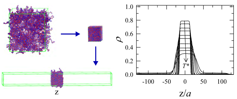
Figure 1: Simulation methodology. The schematic (left) illustrates the computational technique dignon18 ; panag2017 we adopt for calculating phase diagrams of polyampholytes. After energy minimization of a collection of model polyampholytes (chains of red and blue beads) at $T^{*}=4.0$, the cubic simulation box (green frame) with periodic boundary conditions (visualized using VMD vmd with chains at boundaries unwrapped) is compressed under the same high temperature (blue horizontal arrow). This is followed by an expansion (blue vertical arrow) of the simulation box at $T^{*}=1.0$ along the direction (labeled by Cartesian coordinate $z$) of one of its edges, resulting in an enlarged simulation box taking the shape of an elongated rectangular cuboid with a slab of polyampholytes centered at $z=0$. The system is then equilibrated at different temperatures. The plot (right) shows an example of temperature-sensitive equilibrated distributions of polyampholyte density $\rho$ as a function of $z$ (in units of $a$) for the strictly alternating sequence sv1 (refspappu13 ; suman1 , see below). The downward pointing arrow indicates increasing $T^{*}$. For a given temperature, the maximum of the distribution is identified as the polyampholyte density of the condensed phase whereas the minimum as the polyampholyte density of the dilute phase. A phase diagram can thus be constructed from these data. See text for further details.

We begin each simulation by randomly placing $n=500$ IDP chains in a periodic cubic simulation box of length $70a$. Subsequently, the chain configurations are energy-minimized and then heated to a high $T^{*}=4.0$ for $5,000\tau$. This is followed by a compression of the periodic simulation box (by isotropic rescaling of all chain coordinates) at a constant rate under the same high $T^{*}=4.0$ for $10,000\tau$ to arrive at a much smaller periodic cubic box of length $33a$, resulting in a final IDP density $\rho\approx 0.7m/a^{3}$. The simulation box is then expanded along the direction (labeled as $z$) of one of the three axes of the box by a factor of eight with the temperature kept at a low $T^{*}=1.0$, resulting in a simulation box with dimensions $33a\times 33a\times 264a$ containing a concentration of chain population (a “slab”) somewhere along the $z$-axis whereas chain population is zero or extremely sparse for other parts of the elongated simulation box. Any conformation that is originally wrapped in the $z$-direction in the compressed $33a\times 33a\times 33a$ box because of the periodic boundary conditions is unwrapped in this expansion process by placing the chain conformation entirely on the side of the “slab” with larger $z$ values (see Fig. 1 for a visualizationvmd of this procedure).

After this initial preparation, the periodic boundary conditions along the $z$-axis are re-instated. The temperature of the expanded simulation box is changed from $T^{*}=1.0$ to the temperature of interest and equilibrated for $30,000\tau$. The production run is then carried out for $100,000\tau$ during which snapshots of the chain configurations are saved every $10\tau$ for detailed analyses. The position of the simulation box is continuously adjusted such that the center of mass of the chains is always at $z=0$. Density distributions along the $z$ axis are determined by averaging subpopulations of 264 bins of equal width ($=a$) over the simulated trajectories.panag2017 Polyampholytes densities are reported in units of $m/a^{3}$. It follows that the numerical value of $\rho$ is equal to the average number of residues (monomers) in a volume of $a^{3}$. An example of the results from such a calculation is given in Fig. 1.

3.2 Sequence charge pattern parameters

Following Das and Pappu,pappu13 the blockiness parameter $\kappa$ is defined to quantify the deviations of the charge asymmetries of local sequence segments from the overall charge asymmetry of a given sequence. For a sequence segment of length $g$ that starts at monomer $k$ (on any one of the $n$ identical chains labeled by $\mu$), the charge asymmetry is defined as $s(g;k)=[f_{+}(g;k)-f_{-}(g;k)]^{2}/[f_{+}(g;k)+f_{-}(g;k)]$ where $f_{+}(g;k)$ and $f_{-}(g;k)$ are the ratios, respectively, of positively and negatively charged monomers (residues) among the $g$ monomers of the sequence segment; i.e., $f_{\pm}=\sum_{i=k}^{k+g-1}(|\sigma_{\mu i}|\pm\sigma_{\mu i})/2g$ where the summation is over the sequence segment that starts at monomer $k$ and ends at monomer $k+g-1$. It follows that the overall charge asymmetry for the entire sequence with $N$ monomers is $s(N;1)$. The average deviation of local charge asymmetry from the overall charge asymmetry for all $g$-monomer segments (sliding windows) is given by $\delta_{g}\equiv\sum_{k=1}^{N-g+1}[s(g;k)-s(N;1)]^{2}/(N-g+1)$. A $g$-specific quantity $\kappa_{g}\in[0,1]$ is then defined as $\kappa_{g}\equiv\delta_{g}/\max(\delta_{g})$ where $\max(\delta_{g})$ is the maximum $\delta_{g}$ value of the set of sequences with a given composition that is being considered.pappu13 In the present case, $\max(\delta_{g})$ corresponds to the $\delta_{g}$ of the fully charged $N$-monomer diblock polyampholyte. As in refpappu13 , the $\kappa$ we have used for the present work, which takes the form

$$\kappa\equiv\frac{\delta_{5}+\delta_{6}}{{\rm max}(\delta_{5})+{\rm max}(\delta_{6})}\;,$$ (4)

is an average over results for local segment lengths $g=5$ and $g=6$. Note that Eq. (4) differs slightly from the $\kappa=(\kappa_{5}+\kappa_{6})/2$ definition in refpappu13 but the difference is practically negligible ($<1\%$ for low-$\kappa$ sequences and $<0.01\%$ for large-$\kappa$ sequences).

Following Sawle and Ghosh,Sawle15

$${\rm SCD}\equiv\sum_{i=2}^{N}\sum_{j=1}^{i-1}\sigma_{\mu i}\sigma_{\mu j}\sqrt{i-j}/N$$ (5)

is the weighted summation over all pairs of charges along a given sequence.

3.3 Selection of model sequences

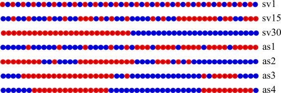
Figure 2: The polyampholyte sequences studied in this work. Every sequence contains 25 K’s (blue beads) and 25 E’s (red beads) with different arrangements of K’s and E’s along the sequences. Sequences sv1, sv15, and sv30 are from refpappu13 ; sequences as1, as2, as3, and as4 are introduced by the present work.

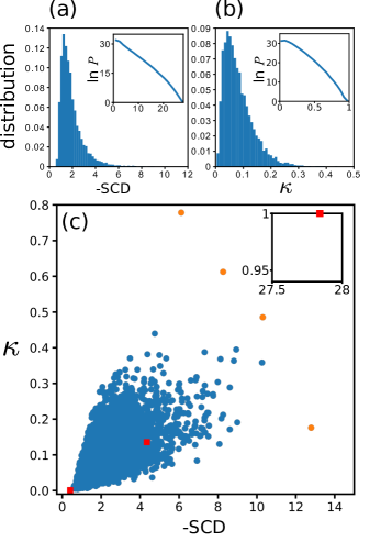
Figure 3: Sequence-space statistics of charge pattern parameters. Normalized distributions of (a) SCD [Eq. (5)] and (b) $\kappa$ [Eq. (4)] among 50-residue fully charged but overall neutral KE sequences are computed from 10,000 sequences generated by repeat exchanges of sequence positions of randomly selected pairs of positive (K) and negative (E) residues. These distributions—histograms in (a,b)—cover only the readily sampled range of SCD and $\kappa$ values, whereas the full distributions of sequence population $P$ over the entire range of all possible SCD and $\kappa$ values are estimated using the Wang-Landau technique WL1 ; WL2 [semi-log plots in the insets of (a) and (b)]. (c) The $-$SCD and $\kappa$ values of the sv1, sv15, sv30 sequences (red squares, bottom to top) and the as1, as2, as3, and as4 sequences (orange circles, bottom to top) are shown against the backdrop of the $-$SCD versus $\kappa$ scatter plot for the 10,000 randomly sampled sequences (blue circles). Sequence sv30 is shown in the inset of (c) because it lies outside the range of the scatter plot. In the histograms in (a) and (b), each of the horizontal ranges between $-$SCD $=0.5640$ and $10.2632$ (a) and that between $\kappa=0.0044$ and $0.4396$ (b) is equally divided into 50 bins. The height of each bar in the histograms is a normalized bin population that is inclusive of the lower boundary but exclusive of the upper boundary of the given bin except it is inclusive of both boundaries for the bin with the largest $-$SCD or $\kappa$. The insets of (a) and (b) are obtained by averaging over ten Wang-Landau processes initialized by different sequences; sampled sequences are binned into 20 equal intervals for the full range of SCD and $\kappa$ values using the same rule for inclusion/exclusion of bin boundaries as described above for the other bins over more limited SCD and $\kappa$ ranges. The scale for population $P$ is such that the sum of all 20 binned populations is equal to the total number, $50!/(25!25!)$, of fully charged 50-residues KE sequences with zero net charge. For the same reason, $P$ is set to unity for the maximum value of $-$SCD and for $\kappa=1$ since both of these parameter values uniquely specify the diblock sv30 sequence. Assuringly, the trend in the inset of (b) is very similar to that exhibited by the previously estimated population distribution over $\kappa$ in Fig S1 of refpappu13 .

We study seven fully charged polyampholyte sequences of length $N=50$. The sequences have equal number of positive and negative residues (charge $\sigma=\pm 1$). Following the nomenclature used in previous studies,pappu13 ; lin2017 ; njp2017 ; suman1 ; Sawle15 we designate the positive and negative residues as “lysine” (K) and “glutamic acid” (E), respectively. The sequences are referred to as “KE” sequences (Fig. 2). Sequences labeled as sv1, sv15, and sv30 were originally introduced in refpappu13 and have been studied previously by theorylin2017 ; njp2017 ; Sawle15 and explicit-chain simulations.pappu13 ; jeetainPNAS ; suman1 These sequences are chosen again for the present study because they span a wide range of values for the sequence charge pattern parameters $\kappa$ and SCD. To provide a context for our simulation study, we have examined the distributions of SCD and $\kappa$ among all possible KE sequences with zero net charge by using simple Monte Carlo as well as Wang-Landau WL1 ; WL2 sampling. The results in Fig. 3a,b indicate that the distributions are concentrated in relatively small $\kappa$ and $-$SCD values. Sequences with large $\kappa$ or large $-$SCD values are extremely rare. A reasonable positive correlation exists between $\kappa$ and $-$SCD; but there is also considerable scatter (Fig. 3c, blue circles), underscoring that the two parameters address similar as well as significantly different sequence properties. Fig. 3c indicates that sv1, sv15, and sv30 lie in a region where $\kappa$ and $-$SCD are well correlated.

RPA theorylin2017 for sv1, sv15, sv30 and 27 other sv sequencespappu13 stipulates that LLPS propensity is well correlated with $\kappa$ and $-$SCD. This prediction is supported to a limited degree by explicit-chain simulation.suman1 In view of these findings, it would be instructive to probe the effectiveness of these charge pattern parameters as LLPS predictors by extending our analysis to outlier sequences that do not exhibit a positive correlation between $\kappa$ and $-$SCD. Because such sequences likely reside in sparely populated regions of sequence space, we use a biased sampling procedure to locate them by maximizing the scoring function

$$E\equiv A\left[-{\rm SCD}/(-{\rm SCD})_{\rm max}-\kappa\right]^{2}+h_{\rm SCD}\left[-{\rm SCD}/(-{\rm SCD})_{\rm max}\right]+h_{\kappa}\kappa\;$$ (6)

for KE sequences, where $A$, $h_{\rm SCD}$, and $h_{\kappa}$ are tunable parameters. When $E$ is maximized, the first term in Eq. (6) maximizes the difference between a rescaled $-$SCD and $\kappa$ ($-{\rm SCD}/(-{\rm SCD})_{\rm max}$, $\kappa$ $\in[0,1]$), whereas the second and third terms control whether a high $-$SCD or a high $\kappa$ value is preferred. Starting with an initial KE sequence, an exchange between a randomly chosen pair of K and E is attempted at each Monte Carlo step. The attempted exchange is accepted if it results in an increase in $E$. Otherwise it is rejected. Partially optimized sequences are generated in this manner by 1,000 Monte Carlo steps. By tuning the $A$, $h_{\rm SCD}$, and $h_{\kappa}$ parameters, we have generated four sequences—labeled by as1, as2, as3, and as4 (Fig. 2)—that collectively exhibit an anti-correlation trend between $\kappa$ and $-$SCD (Fig. 3c, orange circles). The $\kappa$ and SCD values for these sequences and those for the sv1, sv15, and sv30 sequences are summarized in Table 1.

4 Results and Discussion

4.1 Background residue-residue attraction enhances overall LLPS propensity but attenuates the sensitivity of LLPS to charge pattern variation

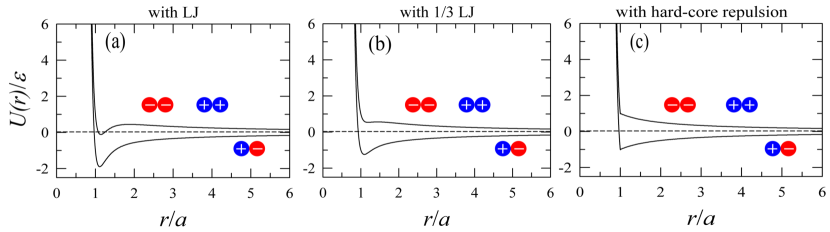
Figure 4: Inter-residue interaction potentials used in our explicit-chain models. In each panel, total interaction energy $U(r)$ in units of $\epsilon$ is shown as a function of inter-residue distance $r$. The upper and lower curves are for a pair of interacting residues with like and opposite charges, respectively, as illustrated by the red- and blue-bead representations of charged residues. The $U(r)=0$ level is marked by a horizontal dotted line. (a) Electrostatics + LJ model [Eq. (1) plus Eq. (2)]. (b) Electrostatics + 1/3 LJ model [Eq. (1) plus 1/3 of Eq. (2)]. (c) Electrostatics + hard-core repulsion model [Eq. (1) plus a modified form of Eq. (2) for which the entire LJ term is set to zero for $r>a$].

For reasons to be expounded below, we consider three different combinations of the electrostatic [$U_{\rm el}$ in Eq. (1)] and LJ [$U_{\rm LJ}$ in Eq. (2)] potentials as the total residue-residue interaction energy $U$ (Fig. 4): (i) simple sum of the two terms, viz., $U=U_{\rm el}+U_{\rm LJ}$ (Fig. 4a); (ii) sum of the electrostatics term and a LJ term reduced to 1/3 of its strength, viz., $U=U_{\rm el}+(1/3)U_{\rm LJ}$ (Fig. 4b); and (iii) sum of the electrostatics term and a LJ term that applies only to $r\leq a$, where $r$ is the residue-residue distance, viz., $U=U_{\rm el}+U_{\rm LJ}$ for $r\leq a$ and $U=U_{\rm el}$ for $r>a$. We are interested in various combinations of $U_{\rm el}$ and $U_{\rm LJ}$ because they bear on one of the formulations used in a general explicit-chain simulation approach to study LLPS of IDPs.dignon18 Here, the “with LJ” model (Fig. 4a) represents a somewhat extreme case in which the LJ attraction is sufficiently strong such that the total interaction remains attractive when the two like charges are in close proximity (for $r\approx 2^{1/6}a$). To address the role of the background LJ interactions on LLPS, the “with 1/3 LJ” model (Fig. 4b) reduces LJ attraction but the overall repulsion between like charges is still considerably weaker than the attraction between opposite charges. In contrast, the “with hard-core repulsion” model (Fig. 4c) retains only the repulsive part of the LJ potential up to the residue-residue separation at which $U_{\rm LJ}=0$ (when $r=a$), such that the strength of repulsion between like charges is equal to that of attraction between opposite charges at $r=a$. This model represents an extreme case in which attractive van der Waals interactions play no role in LLPS. Notably, the symmetry between repulsive and attractive interaction strengths and the treatment of hard-core excluded volume afforded by this model resemble those in RPA theorylinPRL ; linJML (at least conceptually) and in explicit-chain lattice simulations.suman1 It follows that the model potential in Fig. 4c is useful for assessing RPA and lattice results.

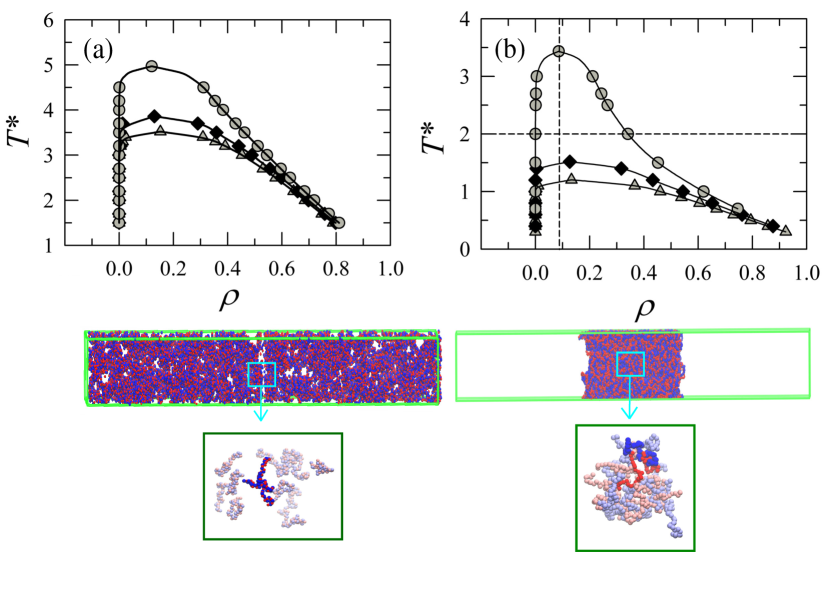
Figure 5: Charge-pattern-dependent phase separations. Phase diagrams are calculated for sequences sv1 (triangles), sv15 (diamonds), and sv30 (circles) using (a) the electrostatics + LJ model potential (Fig. 4a) and (b) the electrostatics + 1/3 LJ model potential (Fig. 4b). Fitted coexistence curves simulated using the present coarse-grained continuum explicit-chain model here and in subsequent figures are constructed as described panag2017 and serve largely as guides to the eye. In (b), the vertical dashed line marks the critical density of sv30 to underscore that it is lower than the critical densities of sv1 and sv15. The horizontal dashed line marks the $T^{*}=2.0$ for which one snapshot of each of the simulation boxes (green frames) for sequence sv1 (left) and for sequence sv30 (right) in (b) are shown below the phase diagrams. Renditions of close-up images (dark-green boxes, bottom) of selected parts of the simulation boxes (blue boxes with arrows) are provided to illustrate key differences in local chain configuration between the two systems. Each of the images in the bottom dark-green boxes consists of one randomly chosen chain and every chain that has either 5 or more (left for sv1) or 15 or more (right for sv30) residues positioned within a distance of $6a$ from a residue of the chosen chain. A pair of such chains are depicted in more saturated color for the sole purpose of enhancing the visual effect.

The phase diagrams for sequences sv1, sv15, and sv30 are calculated using both the “with LJ” and “with 1/3 LJ” models (Fig. 5). All simulated data points in the phase diagrams in this figure and subsequent figures are obtained directly from the density distributions of expanded simulation boxes except the critical points (at the top of each of the coexistence curves) are estimated using the scaling relation specified by Silmore et al.panag2017 Representative chain configurations above and below the critical temperature are provided by the snapshots in Fig. 5. As expected, the model chains exist in a single phase above the critical temperature with essentially uniform polyampholyte density throughout the simulation box (Fig. 5, bottom left). In contrast, a condensed phase (well-defined localized slab in the simulation box) persists below the critical temperature (Fig. 5, bottom right). Consistent with RPA theory njp2017 and lattice simulations,suman1 the critical temperatures [$T^{*}_{\rm cr}({\rm sv1})$, $T^{*}_{\rm cr}({\rm sv15})$, and $T^{*}_{\rm cr}({\rm sv30})$] of the three sequences exhibit a clear increasing trend with increasing $\kappa$ ($=0.0009$, $0.1354$, and $1.000$, respectively) as well as increasing $-$SCD ($=0.413$, $4.349$, and $27.84$, respectively, see Table 1) for both the “with LJ” (Fig. 5a) and “with 1/3 LJ” (Fig. 5b) models. More specifically, $T^{*}_{\rm cr}({\rm sv1})$, $T^{*}_{\rm cr}({\rm sv15})$, and $T^{*}_{\rm cr}({\rm sv30})$ equals, respectively, $3.52$, $3.86$, and $4.97$ in Fig. 5a and $1.20$, $1.52$, and $3.44$ in Fig. 5b.

We expect LLPS propensities to be generally higher in the “with LJ” model (Fig. 5a) than in the “with 1/3 LJ” model (Fig. 5b) because the former model provides a stronger overall residue-residue attraction. This expectation is confirmed by the results in Fig. 5 showing that the $T^{*}_{\rm cr}$’s in Fig. 5a are substantially higher than the $T^{*}_{\rm cr}$’s for the corresponding sequences in Fig. 5b. However, the differences in LLPS properties among the three sequences are more pronounced in the “with 1/3 LJ” model than in the “with LJ” model. Whereas the difference $T^{*}_{\rm cr}({\rm sv15})-T^{*}_{\rm cr}({\rm sv1})$ in the “with LJ” model ($=0.34$) is nearly equal to that in the “with 1/3 LJ” model ($=0.32$), the difference $T^{*}_{\rm cr}({\rm sv30})-T^{*}_{\rm cr}({\rm sv15})$ is substantial smaller in the “with LJ” model ($=1.11$) than in the “with 1/3 LJ” model ($=1.92$). This trend is even more clear when the ratios of $T^{*}_{\rm cr}$’s of different sequences are compared: $T^{*}_{\rm cr}({\rm sv15})/T^{*}_{\rm cr}({\rm sv1})=1.097$ for the “with LJ” model, which is smaller than the corresponding ratio of $1.267$ for the “with 1/3 LJ” model; and $T^{*}_{\rm cr}({\rm sv30})/T^{*}_{\rm cr}({\rm sv15})=1.288$ for the “with LJ” model, which is substantially smaller than the corresponding ratio of $2.263$ for the “with 1/3 LJ” model. These results illustrate that variations in LLPS propensity induced by different sequence charge patterns can be partially suppressed by background residue-residue attraction that pushes the chain molecules to behave more like homopolymers.

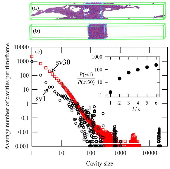
Figure 10: Comparing distributions of cavity size in different polyampholyte-rich states. The associated state of sv1 at $T^{*}=0.001$ in the “electrostatic + hard-core repulsion” model (a) and the condensed phase of sv30 at $T^{*}=0.7$ in the “electrostatics + 1/3 LJ” model (b) are compared by considering 959 and 914 configurational snapshots (timeframes), respectively, for sv1 and sv30 [one snapshot of each set is shown in (a) and (b)]. We focus on their respective volumes of $(33a)^{3}$ with highest average polyampholyte density [indicated by dotted light-blue boxes in (a,b); $z\in[-29a,4a]$ in (a) and $z\in[-16.5a,16.5a]$ in (b)], with periodic boundary conditions maintained within these volumes of $(33a)^{3}$ along $x$ and $y$ but not in the $z$ direction. We consider small cubic volumes of $l^{3}$, where $l=a,2a,\dots,6a$, that are placed at intervals of $a$ in all three spatial directions within these volumes and determine the number of such small cubic volumes that do not contain the center of any of the monomers that make up the polyampholytes. These small cubic volumes are termed empty. The configurational difference between the polyampholyte-rich states of the sv1 and sv30 systems here is characterized by two measures. First, a cavity is identified as a region covering one $l=a$ empty volume (of $a^{3}$) and all $l=a$ empty volumes contiguous to it directly or indirectly (i.e., a given $l=a$ empty volume can only belong to one cavity). The size of cavity is given by the number of contiguous $l=a$ empty volumes. The distribution of cavity volume so defined is given in (c) for sv1 (black open circles) and sv30 (red open squares). Second, the total number, $P$, of positions of empty volumes for various $l$ are counted, and the ratio of $P$ for sv1 to that for sv30 is taken for various $l$ values. The inset in (c) shows $P({\rm sv1})/P({\rm sv30})>1$ and increases sharply with increasing $l$. Hence both measures indicate that there are substantially more cavities of larger volumes for the sv1 system than for the sv30 system analyzed in this figure.

Interestingly, the coexistence curve for sv30 in Fig. 5b exhibits clearly an inflection point on the condensed (right-hand) side such that part of the coexistence curve on this side is concave upward. A hint of upward concavity exists also—though barely discernible–for the coexistence curve for sv30 in Fig. 5a as well as the coexistence curves for sv15 and sv1 in Fig. 5b. In contrast, the entire coexistence curves for sv15 and sv1 in Fig. 5a is convex upward. This observation from explicit-chain simulations are consistent with RPA theory of polyampholytes with zero or near-zero net charge.linPRL ; linJML ; lin2017 Indeed, a systematic RPA study of 30 KE sequences indicates that upward concavity of the condensed side of the coexistence curve decreases with decreasing $-$SCD and decreasing $\kappa$ (Figure 1a of reflin2017 ). Whereas the RPA-predicted concavity is prominent for sv30, it is barely discernible for sv15 and sv1 (Figure 10 of refsuman1 ). This upward concavity of coexistence curves is known to be related to the long spatial range of electrostatic interactions and has been predicted by RPA theory for polyelectrolytes.delaCruz2003 Apparently—and not inconsistent with intuition, LLPS properties of polyampholytes with more blocky sequence charge patterns are in some respect akin to those of polyelectrolytes. Comparison of the coexistence curves in Fig. 5a against those in Fig. 5b suggests further that upward concavity of the coexistence curve is likely associated with the presence of strong long-range repulsive interactions in the system as well. In this regard, it is instructive to note that none of the coexistence curves simulated recently in refsjeetainPNAS ; dignon18 for various intrinsically disordered proteins or protein regions exhibit upward concavity. The only coexistence curve in these references that shows a clear upward-concave trend is the one for a model folded helicase domain in Figure S14 of refdignon18 .

4.2 Sequence charge pattern parameters $\kappa$ and SCD are good predictors of LLPS propensity for some but not all polyampholytes

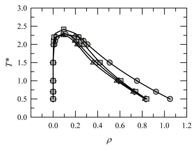
Figure 6: Phase diagrams for the four newly introduced polyampholyte sequences. Simulation results are shown for sequences as1 (triangles), as2 (diamonds), as3 (circles), and as4 (squares), all computed using the electrostatics + 1/3 LJ potential (Fig. 4b). Critical temperature and critical volume are quite insensitive to the variation of charge pattern among these sequences.

As a group, the as1–4 sequences exhibits anti-correlation between $\kappa$ and $-$SCD. In contrast to sequences sv1, sv15, and sv30 in Fig. 5 with $T^{*}_{\rm cr}$ increasing with both increasing $\kappa$ and increasing $-$SCD, the phase diagrams for sequences as1, as2, as3, and as4 in Fig. 6 are quite similar despite their very diverse $\kappa$ values ranging from $0.1761$ for as1 to $0.7783$ for as4 (Table 1). Their $T^{*}_{\rm cr}$’s are 2.25, 2.31, 2.28, and 2.41, respectively. Although $T^{*}_{\rm cr}$ generally increases with $\kappa$ (except for as2 and as3), the increase of $T^{*}_{\rm cr}$ with respect to $\kappa$ is small: From as1 to as4, only a difference of $T^{*}_{\rm cr}({\rm as4})-T^{*}_{\rm cr}({\rm as1})=0.16$ and a ratio of $T^{*}_{\rm cr}({\rm as4})/T^{*}_{\rm cr}({\rm as1})=1.071$ are registered for an increase in $\kappa$ of $0.6022$. By comparison, even though the difference in $\kappa$ is much smaller at $0.1375$ for the sv1 and sv15 sequences, their $T^{*}_{\rm cr}$ difference and ratio simulated using the same “with 1/3 LJ” model (Fig. 5b), $0.32$ and $1.267$ respectively, are much larger than those between as1 and as4 in Fig. 6.

Because of the anti-correlation between $\kappa$ and $-$SCD among sequences as1–4 (Fig. 3c), the $T^{*}_{\rm cr}$’s of the as1–4 sequences in Fig. 6 anti-correlate with their $-$SCD values—rather than correlating with $-$SCD as in the case of the sv1, sv15, and sv30 sequences. Specifically, the increase of the critical temperature from as1 to as4, $T^{*}_{\rm cr}({\rm as4})-T^{*}_{\rm cr}({\rm as1})=0.16$, is accompanied by a decrease in the value of $-$SCD from $12.79$ for as1 to $6.11$ for as4 (a difference of $6.68$). This magnitude of the rate of change of $T^{*}_{\rm cr}$ with respect to SCD is only about a third of that between sequences sv1 and sv15 and is in the opposite direction ($0.32$ change in $T^{*}_{\rm cr}$ from sv1 to sv15 is concomitant with a $-$SCD increase of $3.936$).

The comparison between the results in Fig. 5 and Fig. 6 thus indicates that $\kappa$ and SCD are sensitive predictors of the LLPS of a certain class of polyampholytes (such as the sv1, sv15, and sv30 sequences) but not others (such as the as1, as2, as3, and as4 sequences). This limitation of the $\kappa$ and SCD parameters is not entirely surprising in view of their origins as intuitive pappu13 and theoretial Sawle15 predictors of single-chain conformational dimensions of polyampholytes, not as predictors for LLPS. By construction, $\kappa$ quantifies the degree to which the sequence charge distribution is locally blocky, whereas SCD addresses complementarily sequence-nonlocal effects from charges that are separated by a long segment of the chain. For the original set of 30 polyampholytes introduced in refpappu13 (which includes sv1, sv15, and sv30), SCD correlates better with explicit-chain simulated radius of gyration pappu13 and RPA-predicted $T^{*}_{\rm cr}$’s.lin2017 Now, the $T^{*}_{\rm cr}$’s weak positive correlation with $\kappa$ and weak negative correlation with $-$SCD for the as1–4 sequences in Fig. 6 suggest that the effect of local charge pattern on LLPS—which is a multiple-chain phenomenon—may be stronger than that of nonlocal charge pattern. Nonetheless, the fact that $\kappa$ as a LLPS predictor is much less sensitive when it anti-correlates with $-$SCD suggests at the same time that nonlocal charge pattern effect does have a non-negligible role in LLPS. We will return to this issue below when we present an extensive study of these sequence charge parameters in the context of RPA theory in Sec. 4.5.

4.3 LLPS of polyampholytes in the absence of background non-electrostatic residue-residue attraction may require highly segregated charge patterns

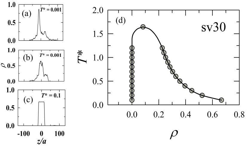
Figure 7: Phase behaviors in the “with hard-core repulsion” model. Polyampholyte density as a function of $z$ is calculated using the model potential in Fig. 4c for (a) sv1, (b) sv15, and (c) sv30 at the temperatures indicated. (d) Phase diagram for sequence sv30 in the same model.

To examine further the effect of background LJ interactions on the sensitivity of LLPS to sequence charge pattern, simulations of sv1, sv15, and sv30 are conducted using the “with hard-core repulsion” model potential in Fig. 4c. Results from this model (Fig. 7) should be more directly comparable with those from pure RPA theory njp2017 (without any Flory $\chi$ parameter linJML ) and lattice simulations suman1 because there is no non-electrostatic attraction in pure RPA theory and our recent explicit-chain lattice model.suman1 Aside from chain connectivity and lattice constraints, the only non-electrostatic interactions in those formulations njp2017 ; suman1 are excluded-volume repulsions. Despite the sharp repulsive forces entailed by this model potential, no erratic dynamics was observed in our Langevin simulations. Nonetheless, it would be instructive in future investigations to assess more broadly the effects of strong intra- and interchain repulsion on phase properties by using Monte Carlo sampling.

Figures 7a,b show the equilibrium density distributions simulated at an extremely low temperature of $T^{*}=0.001$ for sequences sv1 and sv15. This temperature is approaching the lowest that can be practically simulated in the current model, because it is close to the minimum temperature fluctuation that can be maintained by the model thermostat. For example, we have attempted to set the thermostat to $T^{*}=0.0001$ but the actual temperature returned by the simulation was $T^{*}=0.002$. Although the density distributions for sv1 and sv15 in Fig. 7a,b are not uniform throughout their respective simulation boxes—indicating that the chains are to a degree favorably associated with one another, the distributions in Fig. 7a,b do not indicate a clear signature of phase separation,dignon18 ; panag2017 namely a localized, well-defined slab of essentially uniform density (Fig. 1, right). Because a temperature as low as $T^{*}=0.001$ is very unlikely to be physically realizable for a liquid aqueous solution ($T^{*}=0.001$ correspondsnjp2017 to $T\approx 0.5$ K for $\epsilon_{\rm r}=80$ and $T\approx 44$ K for $\epsilon_{\rm r}=1$), we may conclude from Fig. 7a,b that for practical purposes sv1 and sv15 do not undergo LLPS in aqueous solutions in the absence of substantial non-electrostatic attractive interactions.

In contrast, a clear signature of phase separation is indicated for sequence sv30 at a sufficiently low temperature of $T^{*}=0.1$ (Fig. 7c). The simulated phase diagram of sv30 is shown in Fig. 7d. Because of the reduced inter-residue (thus inter-chain) attraction of the “with hard-core repulsion” model (Fig. 4c) relative to the other two model potentials in Fig. 4a,b, the critical temperature $T^{*}_{\rm cr}=1.65$ for sv30 here is lower than the $T^{*}_{\rm cr}$ values of $4.97$ and $3.44$ for sv30 in Fig. 5a and Fig. 5b. The upward concavity of the condensed side of the coexistence curve for sv30 is remarkably more prominent in Fig. 7d than in Fig. 5a and Fig. 5b, buttressing our contention above that this hallmark feature is closely related to the presence of strong repulsive electrostatic interactions in the system.

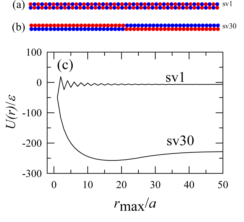
Figure 8: Inter-chain polyampholyte interactions are strongly sequence dependent. A pair of sv1 sequences (a) and a pair of sv30 sequences are each shown in an energetically favorable aligned configuration. (c) Total interaction energy for the configurations in (a) and (b) as functions of the maximum residue-residue distance, $r_{\rm max}$, that is taken into consideration in computing the electrostatic energies.

The dramatic differences in LLPS propensity among the three systems studied in Fig. 7 are illustrated by two extreme cases of a particular energetically favorable configuration for a pair of sv1 chains (Fig. 8a) and one for a pair of sv30 chains (Fig. 8b). In these configurations, inter-chain distances between contacting beads are constant at $r=a$ and thus repulsive LJ energies do not contribute to the total interaction energies plotted in Fig. 8c, which is given by $\sum_{i,j;r_{\mu i,\nu j}\leq r_{\rm max}}(U_{\rm el})_{\mu i,\nu j}$, where $\mu,\nu$ are the labels for the two chains in each pair. Figure 8c shows that the sv30 pair is energetically much more favorable than the sv1 pair. At the large cutoff limit ($r_{\rm max}\to\infty$), the interaction energy for the sv1 pair limits to $-6.5\epsilon$, whereas that for the sv30 pair limits to $-228.2\epsilon$. This difference helps rationalize the lack of LLPS for sv1 and the possibility of LLPS for sv30. The strictly alternating charge pattern of sv1 leads to a very weak net favorable interaction between a sv1 pair even when the pair is in the highly special—and thus unlikely—configuration in Fig. 8a. This is because of numerous partial cancellations of attractions between a pair of opposite charges and repulsions between a pair of like charges since such pairs are positioned next to each other. The weakness of the net favorable inter-chain interaction means that the inter-chain attraction in a highly constrained configuration that can readily be overwhelmed by increased configurational entropy in an ensemble of more open chains. By comparison, for sv30, because of the much stronger net favorable inter-chain interaction, a condensed phase can ensue at a sufficiently low temperauture when the free-energy effect of configurational entropy is relatively diminished.

4.4 Lattice models can overestimate LLPS propensity because of their artefactual spatial order

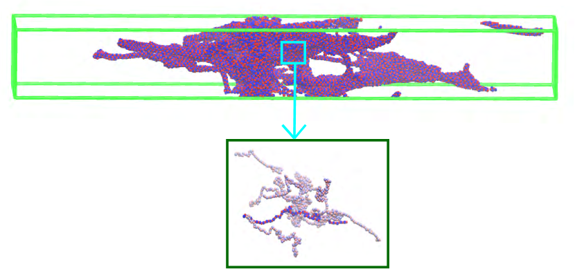
Figure 9: Strictly alternating polyampholytes with hard-core repulsion at extremely low temperature. A snapshot of sv1 chains in a simulation box at $T^{*}=0.01$. The chains are seen as associated and not scattered though there is no clear sign of phase separation (cf. Fig. 7a). The close-up image (bottom) includes all of the chains that have at least one residue within $6a$ of a residue on a randomly selected chain. (The actual number of such $\leq 6a$ inter-chain residue-residue distances varies from 1 to 24 in the chain cluster shown). Two chains inside the bottom box are depicted in more saturated color for the sole purpose of enhancing visualization.

To gain further insight into low-temperature LLPS properties of sv1, a snapshot of sv1 configurations simulated at $T^{*}=0.001$ is shown in Fig. 9. The chains are loosely associated but they do not coalesce into a droplet or a slab in the simulation box. Even the more densely populated region of the simulation box contains region of substantial pure solvent volumes (solvent-filled cavities or “voids” in the model) with no sv1 chains, indicating that the associated state has a very weak effective surface tension and is not liquid-like. The snapshot shows that some individual chain conformations are elongated, presumably to achieve more favorable inter-chain contacts by near parallel alignment (similar to Fig. 8a), but others appear more globular (Fig. 9, bottom). The geometric/configurational difference between the type of associated states in Fig. 9 and unambiguously phase-separated condensed phases such as the one depicted in Fig. 5 (bottom right) may be quantified by the analysis of cavity distributions in Fig. 10, which shows by two different rudimentary measures of cavity size that there are substantially more large solvent-filled cavities in the peculiar associated state in Fig. 9 than in a condensed phase that has clearly undergone phase separation.

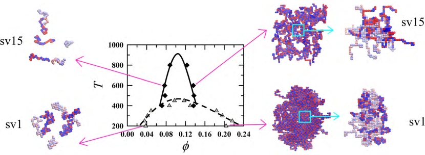
Figure 11: Lattice chain configurations in dilute and condensed phases of phase-separated polyampholytes. The phase diagrams (center) for sv1 (triangles fitted by dashed curve) and for sv15 (diamonds fitted by solid curve) were computed using our previous lattice model and adapted using data from Figure 8 of Das et al.suman1 $T$ is absolute temperature and $\phi$ is polyampholyte volume fraction as described.suman1 Here we provide snapshots of the dilute and of the condensed phases in the lattice model under the simulated $(T,\phi)$ conditions indicated by the red arrows. Snapshots on the dilute side consist of chains in a randomly selected volume within the low-$\phi$ region of the simulation box. Snapshots on the condensed side show substantial fractions of the condensed phases as well as close-up images of parts of them (marked by light boxes with arrows). The close-up images are rendered using the same protocol as that for the bottom-right image in Fig. 5. Selected chains in the snapshots of the dilute state and in the close-up images are depicted in more saturated colors than others for the sole purpose of enhancing visualization.

In contrast to the present continuum simulation results, both sv1 and sv15 were observed to coalesce into a condensed phase in our previous explicit-chain lattice simulation suman1 (Fig. 11). Thus, by comparing explicit-chain simulation results from the present continuum model against those from our previous lattice model, it is clear that the spatial order imposed by the lattice can have a very significant effect in favoring phase separation in lattice model systems. Lattice constraints represent a significant restriction on configurational freedom, allowing opposite charges along polyampholytes to align more optimally. This effect is illustrated by the snaphots for condensed phases in Fig. 11. The above observation implies that lattice models of phase separation can drastically overstimate phase separation propensity in real space. However, in some applications, it may be argued that the lattice order can serve to mimic certain physically realistic local configurational order—such as that induced by hydrogen bonding in protein secondary structure—that is not taken into account in a coarse-grained continuum chain model.chandill90 ; cohen1994 ; yee1994 Chains configured on lattices may also capture certain effects of steric constraints such as those embodied in the tube model of proteins banavar2000 (see footnote 2 on p. S309 of ref wallin2006 ). The degree to which these subtle ramifications of lattice features can be exploited in the study of IDP LLPS remains to be explored. Taken together, these considerations indicate that lattice models can be useful in exploring general principles (Sec. 2) and deserve further attention in future studies; but their predictions should always be interpreted with extra caution.

4.5 RPA theory is useful for physically rationalizing polyampholyte LLPS but has its limitations

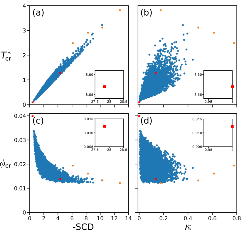
Figure 12: Relationship between RPA-predicted phase properties and sequence charge pattern parameters. RPA-predicted critical temperatures $T^{*}_{\rm cr}$ (a,b) and critical volume fractions $\phi_{\rm cr}$ (c,d) of the 10,000 sampled polyampholyte sequences in Fig. 3 are computed using the salt-free RPA formulationlinPRL (no Flory $\chi$ parameter) and plotted against their $-$SCD (a,c) and $\kappa$ (b,d) values (blue circles). The sequences studied by the present explicit-chain simulations are marked as in Fig. 3 (red squares for sv1, sv15, and sv30; orange circles for as1, as2, as3, and as4) with sequence sv30 shown in the insets.

We utilize the simulated phase properties of the several polyampholyte sequences computed using different model potentials to assess predictions offered by RPA theory. To set the stage, we first establish a broader context of RPA predictions than is currently available. Applying the salt-free RPA formulation for IDP LLPS linPRL that we adapted delaCruz2003 and detailed lin2017 recently, we numerically calculate the critical temperature $T^{*}_{\rm cr}$ and critical volume fraction $\phi_{\rm cr}$ of all 10,000 randomly sampled sequences in Fig. 3 and examine their relationship with the sequence charge parameters $\kappa$ and $-$SCD (Fig. 12). Consistent with previous observations based on more limited datasets,njp2017 ; suman1 RPA-predicted $T^{*}_{\rm cr}$ of polyampholytes with zero net charge exhibits a very good correlation with $-$SCD (tight scatter in Fig. 12a) but a lesser though still substantial correlation with $\kappa$ (broader scatter in Fig. 12b). The RPA-predicted spread of the $\phi_{\rm cr}$ versus $-$SCD scatter for the same set of polyampholytes (Fig. 12c) is also narrower than the corresponding spread of the $\phi_{\rm cr}$ versus $\kappa$ scatter (Fig. 12d); but this difference in scatter between $-$SCD and $\kappa$ is not as pronounced as the corresponding difference in the scatter for $T^{*}_{\rm cr}$ (Fig. 12a,b).

The RPA-predicted dependence of $T^{*}_{\rm cr}$’s and $\phi_{\rm cr}$’s of the sv1, sv15, sv30 sequences on $-$SCD and $\kappa$ (red squares in Fig. 12) is well within the general, most probable trend expected from the 10,000 randomly sampled sequences (blue circles Fig. 12). However, the as1, as2, as3, and as4 sequences (orange circles in Fig. 12) appear to be outliers. These sequences’ deviation from the most probable trend is mild for the $T^{*}_{\rm cr}$ versus $-$SCD (Fig. 12a), the $\phi_{\rm cr}$ versus $-$SCD (Fig. 12c), and the $\phi_{\rm cr}$ versus $\kappa$ (Fig. 12d) scatter plots, but is severe for the $T^{*}_{\rm cr}$ versus $\kappa$ scatter plot (Fig. 12b). It is clear from Fig. 12b that the sign of correlation of the $T^{*}_{\rm cr}$’s of the as1, as2, as3, and as4 sequences is opposite to the overall trend for the 10,000 randomly sampled sequences (Fig. 12b).

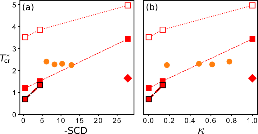
Figure 13: Dependence of explicit-chain-simulated LLPS propensity on sequence charge pattern parameters. The critical temperatures, $T^{*}_{\rm cr}$’s, of 50-residue polyampholytes simulated in the present explicit-chain continuum model are plotted against $-$SCD (a) and $\kappa$ (b) for the “with LJ” potential in Fig. 4a (open squares for sv1, sv15, and sv30), the “with 1/3 LJ” potential in Fig. 4b (filled squares for the three “sv” sequences, filled circles for as1, as2, as3, and as4), and the “with hard-core repulsion” potential in Fig. 4c (diamonds for sv30). The $T^{*}_{\rm cr}$’s of sv1 and sv15 from our previous explicit-chain lattice model simulationsuman1 are also plotted for comparison (red-filled black squares). Dashed and dotted lines joining data points simulated using the same models for sv1, sv15, and sv30 as well as for sv1 and sv15 are merely guides for the eye.

To compare RPA predictions with explicit-chain simulation results, we first summarize the simulation data, by themselves, in Fig. 13, which is the simulation equivalent of the theoretical data in Fig. 12a,b. It provides the dependence of simulated $T^{*}_{\rm cr}$ on the two sequence charge pattern parameters. Figure 13 recapitulates the positive correlation of the simulated $T^{*}_{\rm cr}$’s of the sv1, sv15, and sv30 sequences with $-$SCD and $\kappa$ (squares in Fig. 13). The trends for $-$SCD and $\kappa$ are quite similar. However, in relative terms, the $T^{*}_{\rm cr}$’s of the as1, as2, as3, as4 sequences are almost independent of either $-$SCD and $\kappa$ (circles in Fig. 13). As noted above, the correlation of the $T^{*}_{\rm cr}$ of these four sequences as a set is slightly negative with $-$SCD and only slightly positive with $\kappa$. Only one data point is available in each panel of Fig. 13 for simulated $T^{*}_{\rm cr}$ in the “with hard-core repulsion” model (diamond for sv30) because sv1 and sv15 fail to phase separate unequivocally in this model (see above). The $T^{*}_{\rm cr}$ of sv30 in this model is similar to that of the less-blocky sv15 sequence in the lattice model (red-filled black squares). As stated previously, no simulated $T^{*}_{\rm cr}$ is available for sv30 in our recent lattice model because the favorable interactions in sv30 were too strong for efficient equilibration in that model.suman1

We now contrast our simulation data with theoretical predictions. Depending on the simulation conditions, different matching theoretical formulations are used for the comparison: (i) Pure RPA theory for electrostatic and excluded-volume interactions only, as described in reflinPRL , is utilized to compare with present simulations using the “with hard-core repulsion” potential that does not include any non-electrostatic attraction (Fig. 4c). (ii) The RPA+FH theory prescribed by Equation 10 in reflinPRL with a Flory parameter $\chi=(2\sqrt{2}\pi/3)/T^{*}$ is adopted to compare with simulations using the “with LJ” potential (Fig. 4a). Here the $\chi$ parameter is purely enthalpic. It is introduced to mimic the background enthalpic LJ interaction in the simulations, viz., $\chi=({\rm pairwise\ LJ\ energy})\times({\rm pairwise\ contact\ volume})/(2k_{\rm B}T)$. We approximate pairwise LJ energy by the well depth $\epsilon$, and the pairwise contact volume by that of a sphere with radius $2^{1/6}a$ which is the residue-residue separation at which the LJ energy is $\epsilon$. These approximations lead to $\chi=2\epsilon\sqrt{2}\pi/(3k_{\rm B}T)$ $=(2\sqrt{2}\pi/3)/T^{*}$ because $T^{*}=k_{\rm B}T/\epsilon$ and the volume of the conceptual lattice unit for the Flory-Huggins consideration is $a^{3}$. (iii) The same RPA+FH theory but with $\chi=(2\sqrt{2}\pi/9)/T^{*}$, i.e., 1/3 of the background interaction strength, is applied accordingly to compare with simulations using the “with 1/3 LJ” potential (Fig. 4b). (iv) RPA theory for a screened Coulomb potential, as specified by Equations 2 and 3 of refsuman1 , is used to compare against lattice simulation results for sv1 and sv15 we computed previously using screened electrostatics.suman1

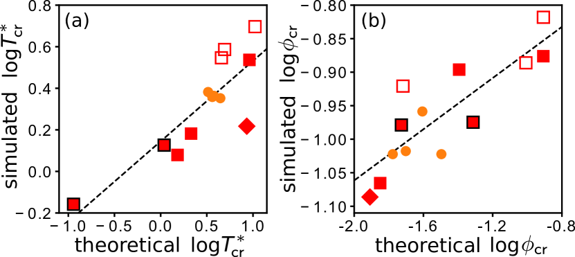
Figure 14: Comparing RPA-predicted and explicit-chain-simulated phase properties of polyampholytes. Simulated logarithmic ($\log=\log_{10}$) critical temperature $T^{*}_{\rm cr}$ (a) and critical volume fraction $\phi_{\rm cr}$ (b) are compared against their theoretical counterparts predicted using RPA or RPA+FH theories. In this figure, $\phi_{\rm cr}$’s for the results simulated in the present study are identified with the simulated $\rho_{\rm cr}$’s (see text and Table 2 for details). The same symbols as those in Fig. 13 are used to specify the sequences and simulation models for the data points. The dashed least-squares regression lines are fitted using all the plotted data points and represent approximate power-law correlations of $T^{*}_{\rm cr}$ or $\phi_{\rm cr}$ between theory and simulation. The lines are given by $\log(T^{*}_{\rm cr,sim})=0.387\log(T^{*}_{\rm cr,thr})+0.145$ in (a) and $\log(\phi_{\rm cr,sim})=0.191\log(\phi_{\rm cr,thr})-0.680$ in (b) where simulated and theoretical quantities are indicated, respectively, by the subscripts “sim” and “thr”. The Pearson correlation coefficients are $0.843$ for (a) and $0.846$ for (b).

Predictions by these theoretical formulations are summarized in Table 2 together with their corresponding simulation results. The theoretical and simulated critical temperatures and critical volume fractions are plotted in Fig. 14. In this theory-simulation comparison, we stipulate that the polyampholyte volume fraction $\phi$ in the simulations may be identified, roughly, to the simulated residue density $\rho$ in Table 2 (hence $\phi_{\rm cr}\approx\rho_{\rm cr}$). By definition, $\rho$ is the average number of residues in a volume of $a^{3}$, thus $\phi\propto\rho$, and the volume of a residue (a bead in the polyampholyte chain model) is $\approx 0.74a^{3}$ (volume of a sphere of radius $2^{1/6}a/2$). It follows that when there is one residue per $a^{3}$ on average (i.e., when $\rho=1$), approximately $0.74$ of the system volume is occupied by van der Waals spheres. With this in mind, since the maximum achievable packing fraction of equal-sized spheres is $\pi/\sqrt{18}\approx 0.74$ also, the maximum packing possible in our simulation system is characterized by $\rho\approx 1$. Thus, $\rho$ is already given in a unit such that it corresponds approximately to the volume fraction $\phi$ ($0\leq\phi\leq 1$) in Flory-Huggins theory.

Figure 14 shows that the simulated $T^{*}_{\rm cr}$ and $\phi_{\rm cr}$ are reasonably correlated with their theoretical counterparts for the sv1, sv15, and sv30 sequences under various simulation conditions. The scatter plots in Fig. 14 suggest two rough scaling relations between simulated (“sim”) and theoretical (“thr”) quantities: $T^{*}_{\rm cr,sim}\sim$ $(T^{*}_{\rm cr,thr})^{0.39}$ and $\phi_{\rm cr,sim}\sim$ $(\phi_{\rm cr,thr})^{0.19}$. The data points for different models in Fig. 14 indicate clearly that these relations hold quite well for the simulated $T^{*}_{\rm cr}$’s and simulated $\phi_{\rm cr}$’s of sv1, sv15, and sv30 for the “with LJ” and “with 1/3 LJ” potentials but they fit poorly with the simulation data of as1, as2, as3, and as4 (for the “with 1/3 LJ” potential) and those of sv30 for the “with hard-core repulsion” potential. That the approximate exponents $0.39$ and $0.19$ in the above scaling relations are both significantly smaller than unity implies that explicit-chain simulated LLPS properties with background LJ, at least as far as $T^{*}_{\rm cr}$ and $\phi_{\rm cr}$ are concerned, are less sensitive to sequence charge pattern than that predicted by RPA+FH theories. However, our finding that sv30 (an outlier in Fig. 14a) can—but sv1 and sv15 cannot—phase separate in the “with hard-core repulsion” model (Fig. 7) suggests that in this case LLPS in explicit-chain models can be even more sensitive to sequence charge pattern than that in RPA. In other words, our results suggest that for polyampholytes that interact only via electrostatics and hard-core excluded-volume repulsion, pure RPA can overstimate LLPS propensity. The case in point here is that while RPA predicts LLPS for sv1 and sv15 with $T^{*}_{\rm cr}$’s that are 0.0104 and 0.149, respectively, of the $T^{*}_{\rm cr}$ of the sv30 sequence,lin2017 ; suman1 the sv1 and sv15 sequences do not phase separate at temperature much lower—as low as $0.001/1.65=6.06\times 10^{-4}$ that of sv30’s $T^{*}_{\rm cr}$—when simulated using the explicit-chain model in Fig. 7.

Figure 14b and Table 2 show that the simulated $\phi_{\rm cr}$’s are larger than their theoretical counterparts for the systems we studied. However, the range of variation is much smaller for the simulated $\phi_{\rm cr}$’s (from $0.082$ to $0.152$) than for the theoretical $\phi_{\rm cr}$’s (from $0.0123$ to $0.124$). It follows that there is a substantial variation in the ratio $\phi_{\rm cr,sim}/\phi_{\rm cr,thr}$ of simulated to theoretical critical volume fraction, from $0.133/0.124=1.07$ for sv1 in the “with 1/3 LJ” model to $0.082/0.0123=6.67$ for sv30 in the “with hard-core repulsion” model. For sequences sv1, sv15, and sv30 simulated using the same interaction scheme, this ratio increases from sv1 to sv15 to sv30, as manifested already by the approximate $\phi_{\rm cr,sim}\sim$ $(\phi_{\rm cr,thr})^{0.19}$ scaling noted above. The large $\phi_{\rm cr,sim}/\phi_{\rm cr,thr}$ ratio for sv30 in the “with hard-core repulsion” model is quantitatively in line with our previous comparison of lattice-simulated and RPA-predicted $\phi_{\rm cr}$’s (Figure 12c of refsuman1 ). In contrast, the smaller $\phi_{\rm cr,sim}/\phi_{\rm cr,thr}$ ratios likely arise from the FH contribution to some of the present theoretical $\phi_{\rm cr}$’s. Pure FH predicts $\phi_{\rm cr}=(\sqrt{N}+1)^{-1}$ [critical $\chi_{\rm cr}=(\sqrt{N}+1)^{2}/(2N)$]. For the current systems with $N=50$, this formula translates to $\phi_{\rm cr}=0.124$, which tends to be significant larger than that predicted by pure RPA.

Echoing the observation that the as1, as2, as3, and as4 sequences are outliers with regard to RPA-predicted properties (Fig. 3c and Fig. 12), these sequences are also outliers in Fig. 14. If linear regression is applied in Fig. 14 to these sequences alone, the correlation coefficient for $T^{*}_{\rm cr}$ in Fig. 14a becomes $r=-0.868$, with a regression slope $-0.204$ that is opposite in sign to that for all the plotted data points (slope $=+0.387$). No clear trend is discernible for these four sequences in the theory-simulation comparison of $\phi_{\rm cr}$ in Fig. 14b ($r=0.198$). (Removing the data points for these four sequences has only very limited effects on the overall linear regressions for Fig. 14a and for Fig. 14b). As emphasized above, the peculiar theoretical and simulated LLPS properties of the as1–4 sequences as well as how these properties are governed by their charge patterns deserve further examination.

5 Conclusions

In summary, we have taken a step to improve the currently limited understanding of the sequence-dependent physical interactions that underlie LLPS of IDPs by extensive simulations of explicit-chain models that allow for a coarse-grained representation of IDP at the residue level, using multiple-chain systems each consisting of 500 individual chains. By analyzing results for 50-residue sequences with diverse charge patterns using model interaction potentials consisting of different combinations of sequence-dependent electrostatics, hard-core excluded-volume repulsion, and LJ attractions, we find that while a general inter-residue LJ attraction—which has a short spatial range—favors LLPS, such a background short-range attraction diminishes sequence specificity of LLPS. Interestingly, and consistent with RPA theory, the condensed side of the coexistence curve of one of the polyampholytes we simulated exhibits a pronounced upward concavity in the absence of background LJ attraction. Such upward concavity is not observed in the presence of strong background LJ interaction or in classical FH theory. This finding suggests that long-range electrostatic repulsion likely allows for condensed phases that are more dilute than when short-range attraction is prominent. This observation should contribute insights into the physical forces that maintain condensed-phase volume fractions of $\approx 0.2$ or even lower.jacob2017 ; low-rho It should be relevant as well for future development of computational and theoretical studies of IDP LLPS that address other sequence-dependent energies biochemrev ; robert beyond electrostatics and LJ-like hydrophobic interactions.dignon18 ; suman1

A main goal of the present study is to use explicit-chain simulations to assess the accuracy of analytical theories and the utility of simple sequence charge pattern parameters $\kappa$ and SCD in capturing LLPS properties of IDPs. The calculation of a pattern parameter for a sequence is virtually instantaneous and numerical calculations for analytical theories are far less computationally intensive than explicit-chain simulations. Therefore, in addition to being tools for elucidating LLPS physics, sequence charge pattern parameters and analytical theories can contribute to efficient high-throughput bioinformatics studies and the screening of candidates in IDP sequence design. Here we have compared and contrasted results simulated for several polyampholyte sequences using the present explicit-chain model against the corresponding analytical theory predictions. A broader context for this evaluation is provided by RPA-predicted critical temperatures and volume fractions we calculated for 10,000 randomly sampled sequences. For three sequences belonging to a previous studied set, the simulated critical temperatures, $T^{*}_{\rm cr}$’s, correlate reasonably well with theoretical predictions and also with the $\kappa$ and SCD parameters. We find that the simulated $T^{*}_{\rm cr}$’s are less sensitive to sequence charge pattern than their theory-predicted counterparts when a substantial background LJ interaction is in play. However, simulated $T^{*}_{\rm cr}$’s can be more sensitive than RPA-predicted $T^{*}_{\rm cr}$’s in the absence of background LJ interaction. In this regard, our results suggest that LLPS propensity can be overestimated by RPA in such cases for sequences with small $\kappa$ and small $-$SCD values. Most notably, for four sequences intentionally generated as outliers in the $\kappa$-SCD relationship, neither $\kappa$ nor SCD is a LLPS predictor with a reliable discriminatory power. This discovery suggests that the effect of blockiness of sequence-local charge pattern on LLPS may be overestimated by $\kappa$, whereas the nonlocal effect of sequence charge pattern on LLPS may be overestimated by SCD. Therefore, a more generally applicable sequence charge pattern parameter for LLPS propensity should be developed to overcome this limitation. All in all, in view of the new questions posed by our findings, there is no shortage of productive avenues of further investigation into the physical basis of biomolecular condensates.

Conflicts of Interest
There are no conflicts of interest to declare.

Acknowledgments
We thank Julie Forman-Kay for helpful discussions. This work was supported by Canadian Institutes of Health Research grants MOP-84281 and NJT-155930, Natural Sciences and Engineering Research Council of Canada Discovery Grant RGPIN-2018-04351, and computational resources provided by SciNet of Compute/Calcul Canada.

References

Table 1. Charge pattern parameters for the sequences studied in this work.

sequence	SCD	$\kappa$
sv1	$-0.413$	$0.0009$
sv15	$-4.349$	$0.1354$
sv30	$-27.84$	$1.0000$
as1	$-12.79$	$0.1761$
as2	$-10.30$	$0.4853$
as3	$-8.266$	$0.6125$
as4	$-6.11$	$0.7783$

Table 2. Simulated and theoretical critical temperatures and critical densities or volume fractions considered in Fig. 12 and Fig. 13. Data for sequences sv1 and sv15 in the lattice model and their theoretical counterparts (last two rows) are obtained from Das et al.suman1 Other data are from the present study.

Potential type	Sequence	Simulation		Theory
		$T^{*}_{\rm cr}$	$\rho_{\rm cr}$	$T^{*}_{\rm cr}$	$\phi_{\rm cr}$
“with LJ”	sv1	3.52	0.152	4.55	0.124
	sv15	3.86	0.130	4.93	0.098
	sv30	4.97	0.120	10.52	0.019
“with 1/3 LJ”	sv1	1.20	0.133	1.52	0.124
	sv15	1.52	0.127	2.14	0.040
	sv30	3.44	0.086	9.14	0.014
	as1	2.25	0.095	4.43	0.017
	as2	2.31	0.096	3.77	0.020
	as3	2.28	0.110	3.63	0.025
	as4	2.41	0.095	3.27	0.032
“with hard-core	sv30	1.65	0.082	8.57	0.0123
repulsion”
screened	sv1	0.70	0.106a	0.114	0.0486
	sv15	1.34	0.105a	1.091	0.0187
aThis quantity equals the simulated critical volume
fraction $\phi_{\rm cr}$ in the lattice model.suman1

Graphical Abstract

References

- (1) C. P. Brangwynne, C. R. Eckmann, D. S. Courson, A. Rybarska, C. Hoege, J. Gharakhani, F. Jülicher and A. A. Hyman, Science, 2009, 324, 1729–1732.
- (2) P. Li, S. Banjade, H.-C. Cheng, S. Kim, B. Chen, L. Guo, M. Llaguno, J. V. Hollingsworth, D. S. King, S. F. Banani, P. S. Russo, Q.-X. Jiang, B. T. Nixon and M. K. Rosen, Nature, 2012, 483, 336–340.
- (3) M. Kato, T. W. Han, S. Xie, K. Shi, X. Du, L. C. Wu, H. Mirzaei, E. J. Goldsmith, J. Longgood, J. Pei, N. V. Grishin, D. E. Frantz, J. W. Schneider, S. Chen, L. Li, M. R. Sawaya, D. Eisenberg, R. Tycko, and S. L. McKnight, Cell, 2012, 149, 753–767.
- (4) T. J. Nott, E. Petsalaki, P. Farber, D. Jervis, E. Fussner, A. Plochowietz, T. D. Craggs, D. P. Bazett-Jones, T. Pawson, J. D. Forman-Kay and A. J. Baldwin, Mol. Cell, 2015, 57, 936–947.
- (5) A. Molliex, J. Temirov, J. Lee, M. Coughlin, A. P. Kanagaraj, H. J. Kim, T. Mittag and J. P. Taylor, Cell, 2015, 163, 123–133.
- (6) Y. Lin, D. S. W. Protter, M. K. Rosen and R. Parker, Mol. Cell, 2015, 60, 208–219.
- (7) E. B. Wilson, Science, 1899, 10, 33–45.
- (8) L. Ehrenberg, Hereditas, 1946, 32, 407–418.
- (9) H. Walter and D. E. Brooks, FEBS Lett., 361, 135–139.
- (10) S. F. Banani, H. O. Lee, A. A. Hyman and M. K. Rosen, Nat. Rev. Mol. Cell Biol., 2017, 18, 285–298.
- (11) Y. Shin and C. P. Brangwynne, Science, 2017, 357, eaaf4382.
- (12) U. S. Eggert, Biochemistry, 2018, 57, 2403–2404.
- (13) C. L. Cuevas-Velazquez and J. R. Dinneny, Curr. Opin. Plant Biol., 2018, 45, 68–74.
- (14) M. Feric, N. Vaidya, T. S. Harmon, D. M. Mitrea, L. Zhu, T. M. Richardson, R. W. Kriwacki, R. V. Pappu and C. P. Brangwynne, Cell, 2016, 165, 1686–1697.
- (15) A. Vovk, C. Gu, M. G. Opferman, L. E. Kapinos, R. Y. H. Lim, R. D. Coalson, D. Jasnow and A. Zilman, eLife, 2016, 5, e10785.
- (16) A. Zilman, J. Mol. Biol., 2018, DOI:10.1016/j.jmb.2018.07.011.
- (17) M. Zeng, Y. Shang, Y. Araki, T. Guo, R. L. Huganir and M. Zhang, Cell, 2016, 166, 1163–1175.
- (18) Z. Feng, M. Zeng, X. Chen and M. Zhang, Biochemistry, 2018, 57, 2530–2539.
- (19) J. A. Riback, C. D. Katanski, J. L. Kear-Scott, E. V. Pilipenko, A. E. Rojek, T. R. Sosnick and D. A. Drummond, Cell, 2017, 168, 1028–1040.
- (20) T. C. Boothby, H. Tapia, A. H. Brozena, S. Piszkiewicz, A. E. Smith, I. Giovannini, L. Rebecchi, G. J. Pielak, D. Koshland and B. Goldstein, Mol. Cell, 2017, 65, 975–984.
- (21) H. Cai, B. Gabryelczyk, M. S. S. Manimekalai, G. Grüber, S. Salentinig and A. Miserez, Soft Matter, 2017, 13, 7740–7752.
- (22) S. Kim, H. Y. Yoo, J. Huang, Y. Lee, S. Park, Y. Park, S. Jin, Y. M. Jung, H. Zeng, D. S. Hwang and Y. Jho, ACS Nano, 2017, 11, 6764–6772.
- (23) C. D. Keating, Acc. Chem. Res., 2012, 45, 2114–2124.
- (24) R. R. Poudyal, F. P. Cakmak, C. D. Keating and P. C. Bevilacqua, Biochemistry, 2018, 57, 2509–2519.
- (25) A. I. Oparin, The Origin of Life, MacMillan Co., New York, 1938.
- (26) F. J. Dyson, J. Mol. Evol., 1982, 18, 344–350.
- (27) F. Dyson, Orgins of Life, Cambridge University Press, New York, 1985.
- (28) D. Srivastava and M. Muthukumar, Macromolecules, 1996, 29, 2324–2326.
- (29) R. K. Das and R. V. Pappu, Proc. Natl. Acad. Sci. U.S.A., 2013, 110, 13392–13397.
- (30) R. K. Das, K. M. Ruff and R. V. Pappu, Curr. Opin. Struct. Biol., 2015, 32, 102–112.
- (31) P. R. Banerjee, A. N. Milin, M. M. Moosa, P. L. Onuchic and A. A. Deniz, Angew. Chem. Int. Ed. Engl., 2017, 56, 11354–11359.
- (32) X.-H. Li, P. L. Chavali, R. Pancsa, S. Chavali and M. M. Babu, Biochemistry, 2018, 57, 2452–2461.
- (33) A. S. Holehouse and R. V. Pappu, Biochemistry, 2018, 57, 2415–2423.
- (34) S. Jain, J. R. Wheeler, R. W. Walters, A. Agrawal, A. Barsic, and R. Parker, Cell, 2016, 164, 487–498.
- (35) I. Kwon, M. Kato, S. Xiang, L. Wu, P. Theodoropoulos, H. Mirzaei, T. Han, S. Xie, J. L. Corden and S. L. McKnight, Cell, 2013, 155, 1049–1060.
- (36) Z. Monahan, V. H. Ryan, A. M. Janke, K. A. Burke, S. N. Rhoads, G. H. Zerze, R. O’Meally, G. L. Dignon, A. E. Conicella, W. Zheng, R. B. Best, R. N. Cole, J. Mittal, F. Shewmaker and N. L. Fawzi, EMBO J., 2017, 36, 2951–2967.
- (37) C. P. Brangwynne, T. J. Mitchison and A. A. Hyman, Proc. Natl. Acad. Sci. U.S.A., 2011, 108, 4334–4339.
- (38) D. Zwicker, R. Seyboldt, C. A. Weber, A. A., Hyman and F. Jülicher, Nat. Phys., 2017, 13, 408–413.
- (39) J. Berry, C. P. Brangwynne and M. Haataja, Rep. Prog. Phys., 2018, 81, 046601.
- (40) J. D. Wurtz and C. F. Lee, New J. Phys., 2018, 20, 045008.
- (41) T. S. Harmon, A. S. Holehouse, M. K. Rosen and R. V. Pappu, eLife, 2017, 6, e30294.
- (42) Y.-H. Lin, J. D. Forman-Kay and H. S. Chan, Biochemistry, 2018, 57, 2499–2508.
- (43) S. C. Weber, Curr. Opin. Cell Biol., 2017, 46, 62–71.
- (44) F. G. Quiroz and A. Chilkoti, Nat. Mater., 2015, 14, 1164–1171.
- (45) L.-W. Chang, T. K. Lytle, M. Radhakrishna, J. J. Madinya, J. Vélez, C. E. Sing and S. L. Perry, Nat. Comm., 2017, 8, 1273.
- (46) J. R. Simon, N. J. Carrol, M. Rubinstein, A. Chilkoti and G. P. López, Nat. Chem., 2017, 9, 509–515.
- (47) K. M. Ruff, S. Roberts, A. Chilkoti and R. V. Pappu, J. Mol. Biol., 2018, DOI:10.1016/j.jmb.2018.06.031.
- (48) A. A. Hyman, C. A. Weber and F. Jülicher, Annu. Rev. Cell Dev. Biol., 2014, 30, 39–58.
- (49) C. P. Brangwynne, P. Tompa and R. V. Pappu, Nat. Phys., 2015, 11, 899–904.
- (50) J. Wang, J. M. Choi, A. S. Holehouse, X. Zhang, M. Jahnel, R. Lemaitre, S. Maharana, A. Pozniakovsky, D. Drechsel, I. Poser, R. V. Pappu, S. Alberti and A. A. Hyman, Cell, 2018, DOI:10.1016/j.cell.2018.06.006.
- (51) A. V. Ermoshkin and M. Olvera de la Cruz, Macromolecules, 2003, 36, 7824–7832.
- (52) Y.-H. Lin, J. D. Forman-Kay and H. S. Chan, Phys. Rev. Lett., 2016, 117, 178101.
- (53) Y.-H. Lin, J. Song, J. D. Forman-Kay and H. S. Chan, J. Mol. Liq., 2017, 228, 176–193.
- (54) Y.-H. Lin and H. S. Chan, Biophys, J., 2017, 112, 2043–2046.
- (55) Y.-H. Lin, J. P. Brady, J. D. Forman-Kay and H. S. Chan, New J. Phys., 2017, 19, 115003.
- (56) G. L. Dignon, W. Zheng, R. B. Best, Y. C. Kim and J. Mittal, Proc. Natl. Acad. Sci. U.S.A., 2018 115, 9929-9934.
- (57) T. K. Lytle and C. E. Sing, Soft Matter, 2017, 13, 7001–7012.
- (58) G. Desjardins, C. A. Meeker, N. Bhachech, S. L. Currie, M. Okon, B. J. Graves and L. P. McIntosh, Proc. Natl. Acad. Sci. U.S.A., 2014, 111, 11019–11024.
- (59) J. Song, S. C. Ng, P. Tompa, K. A. W. Lee and H. S. Chan, PLoS Comput. Biol., 2013, 9, e1003239.
- (60) L. M. Salonen, M. Ellermann amd F. Diederich, Angew. Chem. Int. Ed., 2011, 50, 4808–4842.
- (61) R. M. Vernon, P. A. Chong, B. Tsang, T. H. Kim, A. Blah, P. Farber, H. Lin and J. D. Forman-Kay, eLife, 2018, 7, e31486.
- (62) S. Das, A. Eisen, Y.-H. Lin and H. S. Chan, J. Phys. Chem. B, 2018, 122, 5418–5431.
- (63) S. Das, A. Eisen, Y.-H. Lin and H. S. Chan, J. Phys. Chem. B, 2018, 122, 8111.
- (64) K. M. Ruff, T. S. Harmon and R. V. Pappu, J. Chem. Phys., 2015, 143, 243123.
- (65) Y. S. Harmon, A. S. Holehouse and R. V. Pappu, New J. Phys., 2018, 20, 045002.
- (66) G. L. Dignon, W. Zheng, Y. C. Kim, R. B. Best and J. Mittal, PLoS Comput. Biol., 2018, 14, e1005941.
- (67) K. A. Burke, A. M. Janke, C. L. Rhine and N. L. Fawzi, Mol. Cell, 2015, 60, 231–241.
- (68) J. P. Brady, P. J. Farber, A. Sekhar, Y.-H. Lin, R. Huang, A. Bah, T. J. Nott, H. S. Chan, A. J. Baldwin, J. D. Forman-Kay and L. E. Kay, Proc. Natl. Acad. Sci. USA, 2017, 114, E8194–E8203.
- (69) N. Dorsaz, G. M. Thurston, A. Stradner, P. Schurtenberger and G. Foffi, J. Phys. Chem. B, 2009, 113, 1693–1709.
- (70) M. Kastelic, Y. V. Kalyuzhnyi, B. Hribar-Lee, K. A. Dill and V. Vlachy, Proc. Natl. Acad. Sci. USA, 2015, 112, 6766–6770.
- (71) M. Kastelic, Y. V. Kalyuzhnyi and V. Vlachy, Soft Matter, 2016, 12, 7289–7298.
- (72) A. Stradner, G. Foffi, N. Dorsaz, G. M. Thurston and P. Schurtenberger, Phys. Rev. Lett., 2007, 99, 198103.
- (73) N. Dorsaz, G. M. Thurston, A. Stradner, P. Schurtenberger and G. Foffi, Soft Matter, 2011, 7, 1763–1776.
- (74) V. Nguemaha and H.-X. Zhou, Sci. Rep., 2018, 8, 6728.
- (75) S. Qin and H.-X. Zhou, J. Phys. Chem. B, 2016, 120, 8164–8174.
- (76) S. Qin and H.-X. Zhou, Curr. Opin. Struct. Biol., 2017, 43, 28–37.
- (77) C. Liu, N. Asherie, A. Lomakin, J. Pande, O. Ogun and G. B. Benedek, Proc. Natl. Acad. Sci. U.S.A., 1996, 93, 377–382.
- (78) M. Muschol and F. Rosenberger, J. Chem. Phys., 1997, 107, 1953–1962.
- (79) J. Möller, S. Grobelny, J. Schulze, S. Bieder, A. Steffen, M. Erlkamp, M. Paulus, M. Tolan and R. Winter, Phys. Rev. Lett., 2014, 112, 028101.
- (80) J. Chen, Arch. Biochem. Biophys., 2012, 524, 123–131.
- (81) T. Chen, J. Song and H. S. Chan, Curr. Opin. Struct. Biol., 2015, 30, 32–42.
- (82) R. B. Best, Curr. Opin. Struct. Biol., 2017, 42, 147–154.
- (83) Z. A. Levine and J.-E. Shea, Curr. Opin. Struct. Biol., 2017, 43, 95–103.
- (84) F. J. Blas, L. G. MacDowell, E. de Miguel and G. Jackson, J. Chem. Phys., 2008, 129, 144703.
- (85) K. S. Silmore, M. P. Howard and A. Z. Panagiotopoulos, Mol. Phys., 2017, 115, 320–327.
- (86) G. C. Yeo, F. W. Keeley and A. S. Weiss, Adv. Colloid Interface Sci., 2011, 167, 94–103.
- (87) L. D. Muiznieks and F. W. Keeley, Biochim. Biophys. Acta, 2013, 1832, 866–875.
- (88) E. W. Martin and T. Mittag, Biochemistry, 2018, 57, 2478–2487.
- (89) S. Ambadipudi, J. Biernat, D. Riedel E. Mandelkow and M. Zweckstetter, Nat. Commun., 2017, 8, 275.
- (90) H. Cinar, S. Cinar, H. S. Chan and R. Winter, Chem. Eur. J., 2018, 24, 8286–8291.
- (91) M. S. Moghaddam, S. Shimizu and H. S. Chan, J. Am. Chem. Soc., 2005, 127, 303–316.
- (92) C. L. Dias and H. S. Chan, J. Phys. Chem. B, 2014, 118, 7488–7509.
- (93) H. Krobath, T. Chen and H. S. Chan, Biochemistry, 2016, 55, 6269–6281.
- (94) A. S. Holehouse and R. V. Pappu, Annu. Rev. Biophys., 2018, 47, 19–39.
- (95) L. Sawle and K. Ghosh, J. Chem. Phys., 2015, 143, 085101.
- (96) L. Sawle, J. Huihui and K. Ghosh, J. Chem. Theor. Comput., 2017, 13, 5065–5075.
- (97) T. Firman and K. Ghosh, J. Chem. Phys., 2018, 148, 123305.
- (98) T. Zarin, C. N. Tsai, A. N. Nguyen Ba and A. M. Moses, Proc. Natl. Acad. Sci. U.S.A., 2017, 114, E1450–E1459.
- (99) K. P. Sherry, R. K. Das, R. V. Pappu and D. Barrick, Proc. Natl. Acad. Sci. U.S.A., 2017, 114, E9243–E9252.
- (100) M. Dzuricky, S. Roberts and A. Chilkoti, Biochemistry, 2018, 57, 2405–2414.
- (101) C. Domb, Adv. Chem. Phys., 1969, 15, 229–259.
- (102) P. G. de Gennes, Scaling Concepts in Polymer Physics; Cornell University Press, Ithaca, 1979.
- (103) K. F. Freed, Renormalization Group Theory of Macromolecules; Wiley, New York, 1987.
- (104) H. Kaya and H. S. Chan, Phys. Rev. Lett., 2003, 90, 258104.
- (105) Z. Liu, J. K. Mann, E. L. Zechiedrich and H. S. Chan, J. Mol. Biol., 2006, 361, 268–285.
- (106) T. Chen and H. S. Chan, Phys. Chem. Chem. Phys., 2014, 16, 6460–6479.
- (107) Z. Liu and H. S. Chan, J. Phys. Condens. Matt.. 2015, 27, 354103.
- (108) A. Z. Panagiotopoulos, V. Wong and M. A. Floriano, Macromolecules, 1998, 31, 912–918.
- (109) G. Orkoulas, S. K. Kumar and A. Z. Panagiotopoulos, Phys. Rev. Lett., 2003, 90, 048303.
- (110) D. W. Cheong and A. Z. Panagiotopoulos, Mol. Phys., 2005, 103, 3031–3044.
- (111) S. Rauscher and R. Pomès, eLife, 2017, 6, e26526.
- (112) S. Piana, J. L. Klepeis and D. E. Shaw, Curr. Opin. Struct. Biol., 2014, 24, 98–105.
- (113) S. Rauscher, V. Gapsys, M. J. Gajda, M. Zweckstetter, B. L. de Groot and H. Grubmüller, J. Chem. Theor. Comput., 2015, 11, 5513–5524.
- (114) R. B. Best, W. Zheng and J. Mittal, J. Chem. Theory Comput., 2014, 10, 5113–5124.
- (115) J. Huang, S. Rauscher, G. Nawrocki, T. Ran, M. Feig, B. L. de Groot, H. Grubmüller and A. D. MacKerell, Jr., Nat. Methods, 2017, 14, 71–73.
- (116) P. Robustelli, S. Piana and D. E. Shaw, Proc. Natl. Acad. Sci. U.S.A., 2018, 115, E4758–E4766.
- (117) G. L. Butterfoss, B. Yoo, J. N. Jaworski, I. Chorny, K. A. Dill, R. N. Zuckermann, R. Bonneau, K. Kirshenbaum, V. A. Voelz, Proc. Natl. Acad. Sci. U.S.A., 2012, 109, 14320–14325.
- (118) J. Sun and R. N. Zuckermann, ACS Nano, 2013, 7, 4715–4732.
- (119) J. A. Anderson, C. D. Lorenz and A. Travesset, J. Comput. Phys., 2008, 227, 5342–5359.
- (120) J. Glaser, T. D. Nguyen, J. A. Anderson, P. Liu, F. Spiga, J. A. Millan, D. C. Morse and S. C. Glotzer, Comput. Phys. Commun., 2015, 192, 97–107.
- (121) D. N. LeBard, B. G. Levine, P. Mertmann, S. A. Barr, A. Jusufi, S. Sanders, M. L. Klein and A. Z. Panagiotopoulos, Soft Matter, 2012, 8, 2385–2397.
- (122) A. Trokhymchuk and J. Alejandre, J. Chem. Phys., 1999, 111, 8510–8523.
- (123) D. Duque and L. F. Vega, J. Chem. Phys., 2004, 121, 8611.
- (124) C. J. Mundy, J. I. Siepmann and M. L. Klein, J. Chem. Phys., 1995, 102, 3376–3380.
- (125) M. G. Martin and J. I. Siepmann, J. Chem. Phys. B, 1998, 102, 2569–2577.
- (126) J. P. Nicolas and B. Smit, Mol. Phys., 2009, 100, 2471–2475.
- (127) J. C. Pamies, C. McCabe, P. T. Cummings and L. F. Vega, Mol. Simul., 2010, 29, 463–470.
- (128) M. P. Allen and D. J. Tildesley, Computer Simulation of Liquids, Oxford University Press, New York, 1991.
- (129) W. Humphrey, A. Dalke and K. Schulten, J. Molec. Graphics, 1996, 14, 33–38.
- (130) F. Wang and D. P. Landau, Phys. Rev. E, 2001, 64, 056101.
- (131) D. P. Landau, S.-H. Tsai and M. Exler, Am. J. Phys., 2004, 72, 1294–1302.
- (132) H. S. Chan and K. A. Dill, J. Chem. Phys., 1990, 92, 3118–3135.
- (133) N. G. Hunt, L. M. Gregoret and F. E. Cohen, J. Mol. Biol., 1994, 241, 312–326.
- (134) D. P. Yee, H. S. Chan, T. F. Havel and K. A. Dill, J. Mol. Biol., 1994, 241, 557–573.
- (135) A. Maritan, C. Micheletti, A. Trovato and J. R. Banavar, Nature, 2000, 406, 287–290.
- (136) S. Wallin and H. S. Chan, J. Phys. Condens. Matt., 2006, 18, S307–S328.
- (137) M.-T. Wei, S. Elbaum-Garfinkle, A. S. Holehouse, C. C.-H. Chen, M. Feric, C. B. Arnod, R. D. Priestley, R. V. Pappu and C. P. Brangwynne, Nat. Chem., 2017, 9, 1118–1125.