Viscoelastic shear stress relaxation in two-dimensional glass forming liquids
Abstract
Translational dynamics of two-dimensional glass forming fluids is strongly influenced by soft, long-wavelength fluctuations first recognized by D. Mermin and H. Wagner. As a result of these fluctuations, characteristic features of glassy dynamics, such as plateaus in the mean squared displacement and the self-intermediate scattering function, are absent in two dimensions. In contrast, Mermin-Wagner fluctuations do not influence orientational relaxation and well developed plateaus are observed in orientational correlation functions. It has been suggested that by monitoring translational motion of particles relative to that of their neighbors, one can recover characteristic features of glassy dynamics and thus disentangle the Mermin-Wagner fluctuations from the two-dimensional glass transition. Here we use molecular dynamics simulations to study viscoelastic relaxation in two and three dimensions. We find different behavior of the dynamic modulus below the onset of slow dynamics (determined by the orientational or cage-relative correlation functions) in two and three dimensions. The dynamic modulus for two-dimensional supercooled fluids is more stretched than for three-dimensional supercooled fluids and it does not exhibit a plateau, which implies the absence of glassy viscoelastic relaxation. At lower temperatures, the two-dimensional dynamic modulus starts exhibiting an intermediate time plateau and decays similarly to the three-dimensional dynamic modulus. The differences in the glassy behavior of two- and three-dimensional glass forming fluids parallel differences in the ordering scenarios in two and three dimensions.
Upon approaching the glass transition, a supercooled fluid exhibits a pronounced viscoelastic response with intermediate time elasticity followed by viscous flow. This response implies a two-step decay of the viscoelastic response function, i.e. of the dynamic modulus. When a fluid’s viscosity reaches poise, it appears solid on typical laboratory time scales, and this value of the viscosity is often used to define the glass transition state point. For three dimensional systems, together with pronounced viscoelastic response and increasing of a fluid’s viscosity, one finds that particle’s positions become localized for increasingly longer times Biroli2013 ; Ediger2012 . This localization results in intermediate time plateaus in correlation functions monitoring particles’ translational motion, such as the mean squared displacement and the intermediate scattering function. Flenner and Szamel Flenner2015 used molecular dynamics simulations to show that there is no transient localization of particles in two-dimensional glass-forming liquids. The lack of localization results in an absence of plateaus in the mean squared displacement and the self-intermediate scattering function. This finding has been verified in experiments of quasi-two-dimensional colloidal particles Vivek2017 ; Illing2017 . The absence of transient localization of translational motion originates from soft, long wavelength fluctuations Vivek2017 ; Illing2017 , which were first recognized by D. Mermin and H. Wagner in the context of two-dimensional magnetic systems Mermin1966 and crystalline solids Mermin1968 . Importantly, Mermin-Wagner fluctuations do not strongly influence orientational relaxation. This is consistent with Flenner and Szamel’s finding of a decoupling between translational and orientational relaxation and the presence of well developed plateaus in orientational correlation functions in two dimensions.
It was recently shown that the difference between the two- and three-dimensional glass transition scenarios evident from Flenner and Szamel’s work could be suppressed by monitoring translational motion of particles with respect to their local environment, i.e. their “cage” Vivek2017 ; Illing2017 ; Shiba2018 . This is achieved by introducing “cage-relative” variants of the mean squared displacement and the intermediate scattering function, which use displacements of the particles measured relative to their neighbors. These cage-relative functions exhibit well developed intermediate time plateaus at state points where the orientational correlation functions exhibit plateaus. This observation suggests that to study glassy dynamics of two-dimensional fluids one needs to remove the effects of Mermin-Wagner fluctuations on the translational motion by focusing on cage-relative displacements rather than absolute displacements. The picture that emerged is that when two-dimensional glassy dynamics is viewed in terms of local properties, as in bond angle correlations Flenner2015 ; Vivek2017 , bond-breaking correlations Flenner2016 ; Shiba2012 ; Shiba2016 , or cage-relative displacements Vivek2017 ; Illing2017 ; Shiba2016 , it is quite similar to the three-dimensional glassy dynamics Tarjus2017 .
However, a recent study suggests that two dimensions might play a special role for the glass transition and, therefore, glassy dynamics. Berthier et al. Berthier2018 found that in two dimensions the ideal glass transition, defined as the state point at which the configurational entropy vanishes, occurs at zero temperature, which is in contrast to the vanishing of the configurational entropy at a non-zero temperature in three dimensions Berthier2017 .
In this work, we address a spectacular manifestation of the incipient glass transition found in a laboratory: we study the temperature dependence of the viscoelastic response and of the shear viscosity. To this end, we monitor the dynamic modulus, which is proportional to the shear stress autocorrelation function. We find that in two dimensions, in the temperature regime where translational relaxation does not exhibit typical features of glassy dynamics but orientational and cage-relative translational correlation functions exhibit well developed plateaus, the dynamic modulus does not have a plateau. Thus, in this temperature regime there is no well developed transient elastic response. At lower temperatures, the dynamic modulus develops a plateau signaling emerging viscoelasticity. We also find that the shear viscosity grows slower with decreasing temperature in two dimensions than in three dimensions, and that its growth is decoupled from that of the orientational and cage-relative relaxation times.
Time-dependent viscoelastic response
The time-dependent viscoelastic response is quantified by the dynamic modulus , which is proportional to the shear stress autocorrelation function EvansMorris , , where is the component of the stress tensor (see Materials and Methods). We note that the modulus depends on inter-particle distances rather than on absolute values of particles’ coordinates, and thus conceptually it resembles orientational and cage-relative correlation functions.
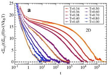
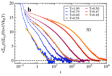
In Fig. 1 we compare the dynamic modulus of model two- and three-dimensional glass-forming systems for temperatures below the onset temperature of slow dynamics (as determined by the appearance of intermediate time plateaus in the orientational and cage-relative correlation functions). We checked by simulating systems of different sizes that there are no finite size effects for the dynamic modulus in two dimensions, in contrast to what was observed for the mean squared displacement and the self-intermediate scattering function Flenner2015 ; Shiba2016 . Upon initial visual inspection, at the lowest temperatures accessible in our simulations, there appears to be little difference in the time dependence of the dynamic modulus for two-dimensional and three-dimensional glass-formers. They both exhibit an initial decay, an intermediate time plateau, and a final decay from the plateau. However, a closer examination of Fig. 1 and a comparison of the temperature dependence of with that of correlation functions sensitive to translational, orientational and cage-relative motions reveals important differences between two and three dimensions.
First, we examine the change of the time dependence of the dynamic modulus upon decreasing temperature in some detail. We fit the final decay to a stretched exponential . The stretching exponent gives deviations from exponential decay, which is expected for three-dimensional liquids well above the onset temperature of slow dynamics. The stretched exponential function fits the final decay well in every case, and three fits are shown in Fig. 1 for both the two-dimensional and the three-dimensional systems. We note that for two-dimensional systems at higher temperatures should only be considered a fit parameter; the fit does not does imply existence of an intermediate time plateau in .
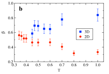
As shown in Fig. 2, we find very different behavior of the amplitude of the stretched exponential fit and of the stretching exponent for two-dimensional and three-dimensional glass forming systems. For two-dimensional glass forming systems at higher temperatures we find that decreases significantly with decreasing temperature, by a factor of 4 between the onset of supercooling and the low temperature limit, and increases by a factor of almost 2. This is in stark contrast to what is observed in three-dimensional systems where is approximately temperature-independent and decreases with decreasing temperature. These observations and a visual inspection of the dynamic modulus shows that stress fluctuations relax differently below the onset of supercooling in two- and three-dimensional systems, but become similar deep within the supercooled liquid. This leads to different viscoelastic relaxation; in two-dimensional glass-forming fluids intermediate-time elastic response appears only upon deep supercooling, whereas in three-dimensional systems it appears just below the onset of slow dynamics.
Shear viscosity
Dramatic increase of the shear viscosity, ,
| (1) |
is a signature of the incipient glass transition. In simulations, the range of the increase is limited to 4 or 5 orders of magnitude. In Fig. 3 we show the shear viscosity for our two- and three-dimensional glass-forming systems. We note that, technically, in two dimensions diverges since there is a long time tail in . However, these (hydrodynamic) long time tails are difficult to observe in simulations of glassy systems. In practice our upper limit of integration is the first time when our calculated crosses zero. In two dimensions, increases by almost 6 orders of magnitude over the full temperature range.
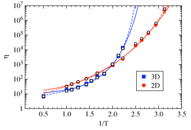
We observe that the shear viscosity of the two-dimensional system increases rather gradually with decreasing temperature below the onset of slow dynamics, in contrast to that of the three-dimensional system. We used two different popular fitting functions, the Vogel-Fulcher fit and the modified Vogel-Fulcher fit , to quantify these temperature dependencies. These fitting functions result in apparent glass transition temperatures and . Note that while we do not assign any fundamental significance to these temperatures, they are useful quantitative characteristics of the onset of solid-like response on macroscopic time scales.
The apparent glass transition temperatures obtained for the two-dimensional glass-former, and , are significantly smaller than those obtained for the three-dimensional glass-former, and . This observation, combined with the fact that the onset of slow dynamics is the same for both systems, agrees with the observation made in the previous section. In two dimensions normal features of glassy viscoelastic behavior are observed only for deeply supercooled systems.
In three-dimensional systems, where the intermediate time plateau appears just below the onset of slow dynamics, viscosity is usually interpreted as a product of the plateau and the characteristic relaxation time of the final decay. Here we make it more quantitative and approximate the viscosity by the integral of the final stretched-exponential decay,
| (2) |
where denotes the Gamma function. As shown in Fig. 3, for all temperature below the onset of slow dynamics, approximation [2] agrees very well with the three-dimensional shear viscosity.
More interestingly, as also shown in Fig. 3, if we apply approximation [2] in two dimensions, the result still agrees very well with the shear viscosity, for all temperatures below the onset of slow dynamics. This happens in spite of the fact that for our two-dimensional glass-former, between the onset of slow dynamics and deep supercooling the dynamic viscosity does not exhibit a clear plateau and the fit parameter is strongly temperature dependent.
Translational, translational cage-relative and orientational dynamic correlation functions
We now compare and contrast temperature dependence of the two-dimensional viscoelastic response with that of the two-dimensional translational, cage-relative, and orientational time-dependent correlation functions.
We start by looking at the self-intermediate scattering function
| (3) |
In Eq. 3 is the position of particle at a time and is the peak position of the static structure factor. The self-intermediate scattering function decay time is a measure of the time it takes for a particle is move over a distance of around . For two-dimensional glass-formers, due to Mermin-Wagner fluctuations, one would expect to decay, albeit possibly very slowly. In contrast, for three-dimensional glass-formers intermediate time localization of the particle positions leads to a pronounced plateau in .
The self-intermediate scattering function is shown in Fig. 4(a)
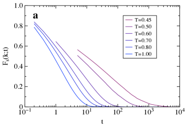
for , 0.8, 0.7, 0.6, 0.5, and 0.45. We note that for temperatures below we could not simulate systems large enough to remove pronounced finite size effects. There is no plateau in the self-intermediate scattering function for the temperature range shown in Fig. 4(a).
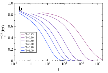
Recently, simulations and experiments analyzing two-dimensional glass-forming systems have examined cage-relative translational dynamics in order to remove the effects of Mermin-Wagner fluctuations Vivek2017 ; Illing2017 ; Shiba2018 . Examining cage-relative motion is motivated by the study of melting of two-dimensional ordered solids. It was argued that by examining cage-relative motion one can remove the size effects shown in the dynamics of two-dimensional simulations, restoring the plateau in the mean squared displacement. Thus, two-dimensional glassy dynamics would then have similar characteristics as three-dimensional glassy dynamics. A cage-relative self-intermediate scattering function
| (4) |
involves the cage-relative displacements
| (5) |
where the summation is over nearest neighbors of particle . For around the peak of the static structure factor, probes the escape of a particle from its cage. Shown in Fig. 4b is for temperatures where we could simulate large enough systems to remove finite size effects, , 0.8, 0.7, 0.6, 0.5, and 0.45. We find that the shape of is similar to what is observed for for three dimensional systems. There is an initial decay to a plateau and then a final decay when the particles begin to lose their neighbors. Additionally, we find that time-temperature super-position holds, i.e. the final decays of overlap if scaled by their relaxation time. This is in stark contrast to the lack of time-temperature superposition for .
However, we recall that there is no plateau in the dynamic modulus for temperatures between and . Thus, by introducing cage-relative function we over-emphasize the glassy character of the dynamics.
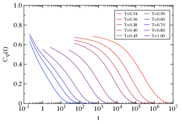
A possible alternative to using cage-relative translational dynamic correlations is provided by an orientational correlation function
| (6) |
In Eq. 6
| (7) |
is the number of neighbors identified through Voronoi tessellation, is the angle that the bond between particle and particle makes with an arbitrary fixed axis at a time . Shown in Fig. 5 is for our full range of temperatures (we verified that there are no finite size effects for ). We clearly see the onset of slow dynamics; at around a plateau emerges. Its height increases slightly with decreasing temperature, but the extent of the plateau and the final relaxation time increase dramatically.
Again, we emphasize that the orientational correlation function exhibits a plateau even when none exists in the dynamic modulus. This is in spite of the fact that both functions depend on interparticle distances and, thus, are only sensitive to local dynamics.
Finally, we comment on the expectation that pronounced finite size effects are removed when one studies cage-relative dynamics. For an ordered two-dimensional solid particles stay within a cage formed by their neighbors. While the absolute position of the particles drifts due to Mermin-Wagner fluctuations, one expects that the position relative to a particles’ neighbors remains fixed.
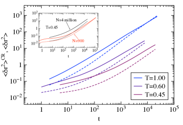
For a glass in two dimensions, we expect that the cage-relative mean squared displacement
| (8) |
will reach a constant value, but will drift due to Mermin-Wagner fluctuations. In a liquid, for long times the displacements are uncorrelated, , and then . Thus, in the long-time limit a liquid’s cage-relative mean squared displacement is larger than the mean squared displacement.
Shown in Fig. 6 is and for , 0.6 and 0.45. There is no plateau in , but there is a plateau in . While the particles displacements are correlated, . Once the particles start to lose their neighbors grows faster than linearly with until is approximately equal to , then grows linearly with . As shown by Shiba et al. Shiba2018 we also find that with for a region of time, but this difference cannot continue to grow in the liquid and eventually it goes through zero.
The cage-relative mean squared displacement is also system size dependent in the liquid state. Shown in the inset to Fig. 6 is and for and calculated for . We can see that and differ at long times. Importantly, there is no finite size effect in the plateau region of . This is in agreement with the observation of Shiba et al. Shiba2018 . These two findings lead us to speculate that in the glass the cage-relative mean squared displacement is not system size dependent.
Time scales
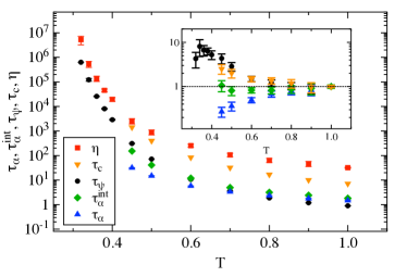
Finally, we briefly compare the growth of the characteristic time scales related to particle motion to that of the shear viscosity. We note that the orientational and cage-relative correlation functions follow time temperature superposition, and thus for these functions we use the usual definition of the relaxation time, and . Since does not obey time temperature superposition, we define two different relaxation times, and .
In Fig. 7 we compare the temperature dependence of the relaxation times and the shear viscosity. There is only about 2 decades in increase of (black circles), (green diamonds), and (orange triangles) over the temperature range where we can calculate these relaxation times. However, we do find that increases faster with decreasing temperature than . This increase is due to the increasingly stretched behavior of . The orientational relaxation time is initially slightly smaller than and , but it increases faster with decreasing temperature. We can calculate over the whole temperature and thus we can see almost 6 orders of magnitude of the orientational relaxation slow down.
To examine the correlations between the relaxation times and the viscosity, we calculate the ratios of the relaxation times to the viscosity. These ratios, normalized to their values at , are shown in the inset to Fig. 7. We find that the cage-relative relaxation time and the orientational relaxation time increase at statistically the same rate and, importantly, they increase faster than the shear viscosity. The former result agrees with the observations of Refs. Vivek2017 and Illing2017 . Thus, available evidence suggests that cage-relative and orientational relaxation are correlated. However, in the temperature range just below the onset of slow dynamics, these dynamics do not seem to be correlated with viscoelastic relaxation.
The integrated relaxation time grows at the same rate as the viscosity, while defined using the standard definition increases slower than viscosity with decreasing temperature. Therefore, at least in the temperature range in which we can simulate large enough systems to remove finite size effects in the self-intermediate scattering function, surprisingly, viscoelastic relaxation seems to be correlated with translational dynamics rather than with orientational relaxation.
Discussion
In two dimensions, low temperature phase behavior and properties of ordered solids are different from those in three dimensions. In particular, the freezing transition can be a two-step process Strandburg1988 ; Halperin1978 ; Nelson1979 ; Young1979 ; with semi-long range orientational correlations appearing first and semi-long range translational correlations and long range (non-decaying) orientational correlations second. Elasticity appears discontinuously at the second transition Strandburg1988 .
We showed here that the two-dimensional glass transition scenario reflects the above described scenario. At the onset of slow dynamics orientational correlations start exhibiting typical features of glassy dynamics: two-step decay with intermediate-time plateau whose duration increases rapidly with decreasing temperature. In contrast, the two-step decay is not seen in the self-intermediate scattering function (which is sensitive to translational relaxation) and in the dynamics modulus (which quantifies viscoelastic relaxation). At a somewhat lower temperature the latter function (the modulus) starts exhibiting typical feature of glassy dynamics. Unfortunately, simulating the self-intermediate scattering function in that temperature range would require using much bigger systems, which is not possible with our present computational resources. We note that on the basis of general arguments invoking Mermin-Wagner fluctuations we expect that translational motion is not localized even in a very deeply supercooled fluid. If the shear viscosity continued to grow as the translational relaxation time, we would expect that the glass transition to occur at . We note that this conclusion, and our modified Vogel-Fulcher fit, is compatible with the result of Berthier et al. Berthier2018 of a zero-temperature transition.
Finally, we elaborate on a remark we made in passing in the section devoted to the shear viscosity. In two dimensions, the very existence of a consistent hydrodynamic description is in question. Specifically, in two dimensions the so-called hydrodynamic long-time tails decay as Resibois . This suggests that the transport coefficients are divergent. Somewhat faster decay is obtained if one does a more advanced self-consistent calculation but the divergence is not eliminated Resibois ; Forster . Here we followed many earlier studies of two-dimensional glassy phenomena and ignored all these effects. From the practical standpoint, the hydrodynamic long-time tails are very difficult to observe in glassy fluids.
I acknowledgements
We gratefully acknowledge partial support of NSF Grant No. DMR-1608086. This research utilized the CSU ISTeC Cray HPC System supported by NSF Grant No. CNS-0923386.
II Simulations
We simulated the Kob-Andersen binary Lennard Jones mixture in two dimensions and three dimensions Kob1994 ; Kob1995a ; Kob1995b . The interaction potential is where , , and . The potential is truncated and shifted at . The results are presented in reduced units where is the unit of length, is the unit of energy, and is the unit of time. The mass is the same for both species. For the three dimensional system the larger species composed 80% of the particles, while the larger species composed of 65% of the particles in the two-dimensional system. We used both LAMMPS and HOOMD blue for the two-dimensional simulations, and LAMMPS for the three dimensional simulations. We simulated temperatures , 0.36, 0.38, 0.4, (in 2D) and 0.45, 0.5, 0.6, 0.7, 0.8, 0.9, and 1.0 (in 2D and 3D). We simulated the system in an NVE ensemble for , but used an NVT Nosé-Hoover thermostat with a coupling constant of . All results are averages over four or more production runs. In 2D, for we simulated particles. We simulated particles for and 4 million particles at . For we again simulated particles. We checked to see if there were finite size effects in the shear stress autocorrelation function and the bond angle correlation function by simulating particles systems at and comparing them with the particle system. The results agreed to within error. In 3D, for all temperatures we simulated particles.
The component of the stress tensor is given by
| (9) |
where is the interaction potential between particle and , and refer to the component of the particle ’s velocity and the projection of the vector , respectively, along the Cartesian axis . The shear stress is the off-diagonal components of . We drop the first term in Eq. [9] since it is small at the temperatures we simulate. The dynamic modulus is proportional to the shear stress autocorrelation function EvansMorris ,
| (10) |
where , is the volume of the simulation cell and is Boltzmann’s constant.
References
- (1) Biroli G, Garrahan JP (2013) Perspective: The glass transition. J Chem Phys 138:12A301.
- (2) Ediger MD, Harrowell P (2012) Perspective: Supercooled liquids and glasses. J Chem Phys 137:080901.
- (3) Flenner E, Szamel G (2015) Fundamental differences between glassy dynamics in two and three dimensions. Nature Commun 6:7392.
- (4) Vivek S, Kelleher CP, Chaikin PM, Weeks ER (2017) Long-wavelength fluctuations and the glass transition in two dimensions and three dimensions. Proc Natl Acad Sci USA 114:1850-1858.
- (5) Illing B, Fritschi S, Kaiser H, Klix CL, Maret G, Keim P (2017) Mermin-Wagner fluctuations in 2D amorphous solids. Proc Natl Acad Sci USA 114:1856-1861.
- (6) Mermin ND, Wagner H (1966) Absence of Ferromagnetism or Anitferromagnetism in One- or Two-Dimensional Isotropic Heisenberg Models. Phys. Rev. Lett. 17:113-1136.
- (7) Mermin ND (1968) Crystalline Order in Two Dimensions. Phys. Rev. 176:250-254.
- (8) Shiba H, Keim P, Kawasaki T (2018) Isolating long-wavelength fluctuation from structural relaxation in two-dimensional glass: cage-relative displacement. J Phys: Condens Matter 30:094004.
- (9) Flenner E, Szamel G (2016) Dynamic heterogeneity in two-dimensional supercooled liquids: comparison of bond-breaking and bond-orientational correlations. J Stat Mech: Theory and Exp 16:074008.
- (10) Shiba H, Kawasaki T, Onuki A (2012) Relationship between bond-breakage correlations and four-point correlations in heterogeneous glassy dynamics: Configuration changes an vibration modes. Phys Rev E 86:041504.
- (11) Shiba H, Yamada Y, Kawasaki T, Kim K (2016) Unveiling Dimensionality Dependence of Glassy Dynamics: 2D infinite Fluctuation Eclipses Inherent Structural Relaxation. Phys Rev Lett 117:245701
- (12) Tarjus G (2017) Glass transitions may be similar in two and three dimensions, after all, Proc Natl Acad Sci USA 114:2440.
- (13) Berthier L, Charbonneau P, Ninarello A, Ozawa M, Yaida S (2018) Zero-temperature glass transition in two dimensions. arXiv:1805.09035.
- (14) Berthier L, Charbonneau P, Coslovich D, Ninarello A, Ozawa M, Yaida S (2017) Configurational entropy measurements in extremely supercooled liquids that break the glass ceiling. PNAS 114:11356-11361.
- (15) Evans DJ, Morris G (2008) Statistical Mechanics of Nonequilibrium Liquids, Cambridge University Press (UK).
- (16) Kob W, Andersen HC (1994) Scaling Behavior in the Beta-Relaxation Regime of a Supercooled Lennard-Jones Mixture. Phys Rev Lett 72:1376-1379.
- (17) Kob W, Andersen HC (1995) Testing Mode-Coupling Theory for a Supercooled Binary Lennard-Jones Mixture-The Van Hove Correlation-Function. Phys Rev E 51:4626-4641.
- (18) Kob W, Andersen HC (1995) Testing Mode-Coupling Theory for a Supercooled Binary Lennard-Jones Mixture 2. Intermediate Scattering Function and Dynamic Susceptibility. Phys Rev E 52:4134-4153.
- (19) Strandburg KJ (1988) Two-dimensional melting. Rev Mod Phys 60:161-207.
- (20) Halperin BI, Nelson DR (1978) Theory of Two-Dimensional Melting. Phy Rev Lett 41:121-124.
- (21) Nelson DR, Halperin BI (1979) Dislocation-mediated melting in two dimensions. Phy Rev B 19:2457-2484.
- (22) Young AP (1979) Melting and the vector Coulomb gas in two dimensions. Phy Rev B 19:1855-1866.
- (23) Résibois P, de Leener M, Classical Kinetic Theory of Fluids (Wiley, New York, 1977).
- (24) Forster D, Nelson DR, Stephen MJ, (1977) Large-distance and long-time properties of a randomly stirred fluid. Phy Rev A 16:732-749.