Environment induced pre-thermalization in the Mott-Hubbard model

Abstract

Via the hierarchy of correlations, we study the strongly interacting Fermi-Hubbard model in the Mott insulator state and couple it to a Markovian environment which constantly monitors the particle numbers $\hat{n}_{\mu}^{\uparrow}$ and $\hat{n}_{\mu}^{\downarrow}$ for each lattice site $\mu$. As expected, the environment induces an imaginary part $\gamma$ (i.e., decay rate) of the quasi-particle frequencies $\omega_{\mbox{\boldmath$\scriptstyle k$}}\to\omega_{\mbox{\boldmath$\scriptstyle k$}}-i\gamma$ and tends to diminish the correlations between lattice sites. Surprisingly, the environment does also steer the state of the system on intermediate time scales $\,{\cal O}(1/\gamma)$ to a pre-thermalized state very similar to a quantum quench (i.e., suddenly switching on the hopping rate $J$). Full thermalization occurs via local on-site heating and takes much longer.

Introduction

Understanding the quantum dynamics of strongly interacting many-body systems is one of the major challenges of contemporary physics. Compared to weakly or non-interacting systems, strong interactions can induce new and fascinating phenomena. One example is the Mott insulator state: For a fermionic lattice with a half-filled band, one would expect conducting (i.e., metallic) behavior – but strong interactions can make this system insulating H63 ; IFT .

While the ground or thermal equilibrium state of strongly interacting systems can already display non-trivial properties, their non-equilibrium dynamics can pose even more difficult problems, which we are just beginning to understand. A conceptually clear and frequently studied example is a quantum quench, where one starts in the ground state of a given Hamiltonian and then suddenly (or non-adiabatically) changes one of the parameters of this Hamiltonian. After that, the initial state will no longer be the ground state in general and the time dependence after such a global excitation has been studied in various works, see, e.g. CC06 ; MWNM07 ; IC09 ; SF11 ; MK08 ; EKW09 ; KLA07 ; BKL10 ; R09 ; R10 ; CDEO08 ; CFMSE08 ; FCMSE08 ; LK08 ; BRK11 ; BPBRK12 ; BPCK12 ; QKNS14 ; NS10 ; NQS14 .

One of the surprises and unexpected results of such non-equilibrium dynamics is the phenomenon of pre-thermalization: Even in systems which are expected to thermalize after a global excitation, this thermalization dynamics can occur in several stages with different time-scales. Local observables which oscillate on short time scales (after the quench) approach a quasi-static value on intermediate time-scales – which is, however, different from their thermal value. Full thermalization (if it occurs) requires much longer time scales. As an intuitive picture, pre-thermalization can be understood as dephasing of the quasi-particle excitations while full thermalization requires the exchange of energy and momentum between the quasi-particles. How strongly interacting quantum many-body systems equilibrate is a very important and not fully solved question which has far reaching consequences, ranging from solid-state devices such as the proposed Mott transistor or other switching processes to the observability of quark-gluon plasma or cosmology.

So far, equilibration and thermalization dynamics after quantum quenches and related questions were mostly discussed in closed quantum systems undergoing a unitary evolution MWNM07 ; IC09 ; MK08 ; EKW09 ; KLA07 ; BKL10 ; R09 ; R10 ; CDEO08 ; CFMSE08 ; FCMSE08 ; QKNS14 . However, every real system is always coupled to an environment, which can also affect the equilibration and thermalization dynamics. In order to fill this gap, we consider a prototypical example for a strongly interacting quantum many-body system and study its non-equilibrium dynamics after coupling it an environment which is assumed to be Markovian.

The Model

The lattice system under consideration is described by the Fermi-Hubbard Hamiltonian ($\hbar=1$)

$$\hat{H}=-\frac{1}{Z}\sum\limits_{\mu,\nu,s}J_{\mu\nu}\hat{c}_{\mu,s}^{\dagger}\hat{c}_{\nu,s}+U\sum\limits_{\mu}\hat{n}_{\mu}^{\uparrow}\hat{n}_{\mu}^{\downarrow}\,,$$ (1)

where $\hat{c}_{\mu,s}^{\dagger}$ and $\hat{c}_{\nu,s}$ are the fermionic creation and annihilation operators for the spin $s\in\{\uparrow,\downarrow\}$ at the lattice sites $\mu$ and $\nu$, respectively. The corresponding hopping rate is denoted by $J_{\mu\nu}$, where we have factored out the coordination number $Z$. The second term describes the on-site repulsion $U$ with the particle number operators $\hat{n}_{\mu}^{\uparrow}$ and $\hat{n}_{\mu}^{\downarrow}$. As possible experimental realizations, one could envision fermionic atoms in optical lattices E10 ; JSGME08 ; CNLOZ16 ; BHSON16 ; PMCJGG16 or electrons in solid state settings LNW06 ; DHS03 .

The above Hamiltonian (1) generates the internal unitary evolution while the coupling to the Markovian environment is described in terms of a master equation with the Lindblad operators $\hat{n}_{\mu,s}$ and the coupling strength $\gamma$

$$\partial_{t}\hat{\rho}=i\left[\hat{\rho},\hat{H}\right]+\gamma\sum\limits_{\mu,s}\left(\hat{n}_{\mu,s}\,\hat{\rho}\,\hat{n}_{\mu,s}-\left\{\hat{n}_{\mu,s},\hat{\rho}\right\}\right)\,,$$ (2)

where we have used $\hat{n}_{\mu,s}^{2}=\hat{n}_{\mu,s}$ for fermions. Thus, the environment permanently monitors (i.e., weakly measures) the number of particles $\hat{n}_{\mu,s}$ per lattice site $\mu$ for each spin species $s$. Such an environment could be represented by a bath of bosons which scatter at the fermions depending on their position. For atoms in optical lattices, they could be photons, and for electrons in solids, they could be phonons, for example.

The above master equation (2) can be written in terms of Liouville super operators

$$\partial_{t}\hat{\rho}=\frac{1}{Z}\sum\limits_{\mu,\nu}{\mathfrak{L}}_{\mu,\nu}\hat{\rho}+\sum\limits_{\mu}{\mathfrak{L}}_{\mu}\hat{\rho}\,,$$ (3)

where ${\mathfrak{L}}_{\mu,\nu}$ contains the hopping term $\propto J_{\mu\nu}$ from (1) while the on-site interaction term $\propto U$ from (1) as well as the environment contribution $\propto\gamma$ from (2) are encoded in the local contribution ${\mathfrak{L}}_{\mu}$.

Hierarchy of Correlations

Since the dynamics (2) can only be solved exactly for very small lattices (see below), we have to introduce a suitable approximation scheme. Here, we employ the hierarchy of correlations QKNS14 ; KNQS14 ; NQS14 ; QNS12 ; NQS16 ; NS10 and consider the reduced density matrices $\hat{\rho}_{\mu}$ for one site and $\hat{\rho}_{\mu\nu}$ for two sites etc. After splitting off the correlations via $\hat{\rho}_{\mu\nu}^{\rm corr}=\hat{\rho}_{\mu\nu}-\hat{\rho}_{\mu}\hat{\rho}_{\nu}$ and so on, we obtain for the evolution of the on-site density matrix

$$\partial_{t}\hat{\rho}_{\mu} = \frac{1}{Z}\sum\limits_{\nu}{\rm Tr}_{\nu}\left\{{\mathfrak{L}}_{\mu,\nu}\hat{\rho}_{\mu}\hat{\rho}_{\nu}+{\mathfrak{L}}_{\mu,\nu}\hat{\rho}_{\mu\nu}^{\rm corr}\right\}+{\mathfrak{L}}_{\mu}\hat{\rho}_{\mu}$$ (4)

$$= f_{1}(\hat{\rho}_{\nu},\hat{\rho}_{\mu\nu}^{\rm corr})\,.$$

In analogy, the time evolution of the two-site correlations can be derived from (3) and also depends on the on-site density matrices as well as the three-site correlators

$$\partial_{t}\hat{\rho}_{\mu\nu}^{\rm corr}=f_{2}(\hat{\rho}_{\nu},\hat{\rho}_{\mu\nu}^{\rm corr},\hat{\rho}_{\mu\nu\sigma}^{\rm corr})\,.$$ (5)

In order to truncate this infinite set of recursive equations, we exploit the hierarchy of correlations in the formal limit of large coordination numbers $Z\gg 1$. With completely the same arguments as in NS10 , it can be shown that the two-site correlations are suppressed via $\hat{\rho}_{\mu\nu}^{\rm corr}=\,{\cal O}(1/Z)$ in comparison to the on-site density matrix $\hat{\rho}_{\mu}=\,{\cal O}(Z^{0})$ and the three-site correlators even stronger via $\hat{\rho}_{\mu\nu\sigma}^{\rm corr}=\,{\cal O}(1/Z^{2})$, and so on. Note that the derivation in NS10 works in completely the same way here because the environment acts locally, i.e., on each lattice site separately, and thus only changes the local Liovillian ${\mathfrak{L}}_{\mu}$ in (3).

This hierarchy of correlations facilitates the following iterative approximation scheme: To zeroth order in $1/Z$, we may approximate (4) via $\partial_{t}\hat{\rho}_{\mu}\approx f_{1}(\hat{\rho}_{\nu},0)$ which yields the mean-field solution $\hat{\rho}_{\mu}^{0}$. As the next step, we may insert this solution $\hat{\rho}_{\mu}^{0}$ into (5) and obtain to first order in $1/Z$ the following approximate set of linear and inhomogeneous equations for the correlations

$$\partial_{t}\hat{\rho}_{\mu\nu}^{\rm corr}\approx f_{2}(\hat{\rho}_{\nu}^{0},\hat{\rho}_{\mu\nu}^{\rm corr},0)\,.$$ (6)

The solution of this set of equations describes the propagation (and damping) of the quasi-particles, insertion back into (4) then yields their back-reaction onto the mean field.

Mean-field Ansatz

Let us study the propagation (and damping) of the quasi-particles according to (6) for a concrete example. For the mean-field solution $\hat{\rho}_{\mu}^{0}$, we assume a homogeneous and spin-symmetric (i.e., unpolarized) state, which can be described by the general ansatz

$$\hat{\rho}_{\mu}^{0}=p_{0}\left|0\right>\left<0\right|+p_{1}\left(\left|\uparrow\right>\left<\uparrow\right|+\left|\downarrow\right>\left<\downarrow\right|\right)+p_{2}\left|\uparrow\downarrow\right>\left<\uparrow\downarrow\right|\,,$$ (7)

with the probabilities for zero $p_{0}$, one $p_{1}$, and two particles $p_{2}$ on the lattice site $\mu$. For the Fermi-Hubbard Hamiltonian (1) and the Lindblad operators $\hat{n}_{\mu,s}$ in (2), this ansatz automatically satisfies the zeroth-order (mean-field) equation $\partial_{t}\hat{\rho}_{\mu}^{0}=f_{1}(\hat{\rho}_{\mu}^{0},0)$.

Since we want to include the Mott insulator state SDM00 ; IFT , we assume half filling $\langle\hat{n}_{\mu}^{\uparrow}+\hat{n}_{\mu}^{\downarrow}\rangle=2p_{1}+2p_{2}=1$. Together with the normalization $p_{0}+2p_{1}+p_{2}=1$, this fixes all probabilities except one, which can be parametrized by the double occupancy $\mathfrak{D}=\langle\hat{n}_{\mu}^{\uparrow}\hat{n}_{\mu}^{\downarrow}\rangle=p_{2}$. It vanishes in the Mott insulator state $p_{0}=p_{2}=0$, but in the infinite-temperature limit $p_{0}=p_{1}=p_{2}$, it tends to 1/4.

Note that, since the ansatz (7) obeys the zeroth-order (mean-field) equation $\partial_{t}\hat{\rho}_{\mu}^{0}=f_{1}(\hat{\rho}_{\mu}^{0},0)$, the double occupancy $\mathfrak{D}$ is constant to lowest order (in $1/Z$). However, including the back-reaction of the quasi-particles and their quantum or thermal fluctuations onto the mean field, it will change in general (see below).

Quasi-particles

Inserting the ansatz (7) into the equation (6) for the correlations, we find the following set of relevant correlation functions, see also QKNS14

$$f^{00}_{\mu\nu,s} = \langle\hat{c}_{\mu,s}^{\dagger}(1-\hat{n}_{\mu,\bar{s}})\,\hat{c}_{\nu,s}(1-\hat{n}_{\nu,\bar{s}})\rangle$$

$$f^{01}_{\mu\nu,s} = \langle\hat{c}_{\mu,s}^{\dagger}(1-\hat{n}_{\mu,\bar{s}})\,\hat{c}_{\nu,s}\hat{n}_{\nu,\bar{s}}\rangle$$

$$f^{10}_{\mu\nu,s} = \langle\hat{c}_{\mu,s}^{\dagger}\hat{n}_{\mu,\bar{s}}\,\hat{c}_{\nu,s}(1-\hat{n}_{\nu,\bar{s}})\rangle$$

$$f^{11}_{\mu\nu,s} = \langle\hat{c}_{\mu,s}^{\dagger}\hat{n}_{\mu,\bar{s}}\,\hat{c}_{\nu,s}\hat{n}_{\nu,\bar{s}}\rangle\,,$$ (8)

with $s\in\{\uparrow,\downarrow\}$ denoting the spin and $\bar{s}$ the opposite spin. All other correlators vanish to first order (in $1/Z$).

As we obtain the same dynamics for both spin species $s$, we omit the spin index $s$ in the following. Assuming spatial homogeneity, we Fourier transform the above correlation functions and (6) becomes

$$\left(i\partial_{t}+i\gamma\right)f^{00}_{\mbox{\boldmath$\scriptstyle k$}} = \frac{J_{\mbox{\boldmath$\scriptstyle k$}}}{2}\left(f^{10}_{\mbox{\boldmath$\scriptstyle k$}}-f^{01}_{\mbox{\boldmath$\scriptstyle k$}}\right)=-\left(i\partial_{t}+i\gamma\right)f^{11}_{\mbox{\boldmath$\scriptstyle k$}}$$

$$\left(i\partial_{t}-U+i\gamma\right)f^{01}_{\mbox{\boldmath$\scriptstyle k$}} = \frac{J_{\mbox{\boldmath$\scriptstyle k$}}}{2}\left(f^{11}_{\mbox{\boldmath$\scriptstyle k$}}-f^{00}_{\mbox{\boldmath$\scriptstyle k$}}\right)-\frac{J_{\mbox{\boldmath$\scriptstyle k$}}}{4}\left(1-4{\mathfrak{D}}\right)$$ (9)

$$= -\left(i\partial_{t}+U+i\gamma\right)f^{10}_{\mbox{\boldmath$\scriptstyle k$}}\,.$$

For time-independent parameters $\gamma$, $J_{\mbox{\boldmath$\scriptstyle k$}}$, $U$, and $\mathfrak{D}$, we may diagonalize the above linear system of equations and thereby obtain four eigen-frequencies, two of them read

$$\omega^{\pm}_{\mbox{\boldmath$\scriptstyle k$}}=\pm\sqrt{U^{2}+J_{\mbox{\boldmath$\scriptstyle k$}}^{2}}-i\gamma$$ (10)

while the other two simply are $\omega^{0}_{\mbox{\boldmath$\scriptstyle k$}}=-i\gamma$. We see that all eigen-frequencies acquire the same imaginary part $-i\gamma$ which just corresponds to an exponential decay $e^{-\gamma t}$. This describes the damping of the quasi-particles induced by the coupling to the environment.

Pre-thermalization

Due to this exponential decay $e^{-\gamma t}$, the correlation functions approach the following asymptotic state (again assuming that $\mathfrak{D}$ is constant)

$$f^{00}_{\mbox{\boldmath$\scriptstyle k$},\rm asy} = -\frac{J_{\mbox{\boldmath$\scriptstyle k$}}^{2}}{U^{2}+J_{\mbox{\boldmath$\scriptstyle k$}}^{2}+\gamma^{2}}\,\frac{1-4{\mathfrak{D}}}{4}=-f^{11}_{\mbox{\boldmath$\scriptstyle k$},\rm asy}\,,$$

$$f^{01}_{\mbox{\boldmath$\scriptstyle k$},\rm asy} = -\frac{J_{\mbox{\boldmath$\scriptstyle k$}}\left(U+i\gamma\right)}{U^{2}+J_{\mbox{\boldmath$\scriptstyle k$}}^{2}+\gamma^{2}}\,\frac{1-4{\mathfrak{D}}}{4}=\left(f^{10}_{\mbox{\boldmath$\scriptstyle k$},\rm asy}\right)^{*}\,,$$ (11)

which is independent of the initial state, i.e., the initial values $f^{00}_{\mbox{\boldmath$\scriptstyle k$}}(t=0)$, $f^{01}_{\mbox{\boldmath$\scriptstyle k$}}(t=0)$, $f^{10}_{\mbox{\boldmath$\scriptstyle k$}}(t=0)$, and $f^{11}_{\mbox{\boldmath$\scriptstyle k$}}(t=0)$. As one would expect, the correlations are suppressed for large $\gamma$ and go to zero in the limit $\gamma\to\infty$.

However, it is interesting to note that this asymptotic state (Pre-thermalization) is different from the ground state, even for $\gamma=0$ and ${\mathfrak{D}}=0$, where we have

$$f^{00}_{\mbox{\boldmath$\scriptstyle k$},\rm ground}=\frac{1}{4}\left(\frac{U}{\sqrt{U^{2}+J_{\mbox{\boldmath$\scriptstyle k$}}^{2}}}-1\right)=-f^{11}_{\mbox{\boldmath$\scriptstyle k$},\rm ground}\,.$$ (12)

Already for small $J_{\mbox{\boldmath$\scriptstyle k$}}$, we observe a factor of two difference to the asymptotic state (Pre-thermalization), see also MK09 ; QKNS14 .

In fact, in the limit of small $\gamma$, the above asymptotic state (Pre-thermalization) coincides with the pre-thermalized state after a quantum quench, where one starts in the ground state with $J=0$ and then suddenly switches on $J$ to its final value, see, e.g., QKNS14 . This coincidence seems to be a rather general property. To understand why, let us write the linear system of equations (Quasi-particles) in matrix form

$$\partial_{t}\mbox{\boldmath$f$}_{\mbox{\boldmath$\scriptstyle k$}}=\mbox{\boldmath$M$}_{\mbox{\boldmath$\scriptstyle k$}}\cdot\mbox{\boldmath$f$}_{\mbox{\boldmath$\scriptstyle k$}}-\gamma\mbox{\boldmath$f$}_{\mbox{\boldmath$\scriptstyle k$}}+\mbox{\boldmath$s$}_{\mbox{\boldmath$\scriptstyle k$}}\,,$$ (13)

with a time-idependent matrix $\mbox{\boldmath$M$}_{\mbox{\boldmath$\scriptstyle k$}}$ describing the Hamiltonian evolution, i.e., depending on $J_{\mbox{\boldmath$\scriptstyle k$}}$ and $U$. Neglecting back-reaction, i.e., assuming that the double occupancy $\mathfrak{D}=\langle\hat{n}_{\mu}^{\uparrow}\hat{n}_{\mu}^{\downarrow}\rangle$ is time-independent, the source term $\mbox{\boldmath$s$}_{\mbox{\boldmath$\scriptstyle k$}}$ is also constant. Then, due to the damping term $\gamma$, the correlations approach the asymptotic state

$$\mbox{\boldmath$f$}_{\mbox{\boldmath$\scriptstyle k$}}^{\rm asy}=\left(\gamma\mbox{\boldmath$1$}-\mbox{\boldmath$M$}_{\mbox{\boldmath$\scriptstyle k$}}\right)^{-1}\cdot\mbox{\boldmath$s$}_{\mbox{\boldmath$\scriptstyle k$}}\,.$$ (14)

Now, the limit $\gamma\to 0$ could be problematic if the source term $\mbox{\boldmath$s$}_{\mbox{\boldmath$\scriptstyle k$}}$ would have contributions in the kernel ${\rm ker}(\mbox{\boldmath$M$}_{\mbox{\boldmath$\scriptstyle k$}})$ of the matrix $\mbox{\boldmath$M$}_{\mbox{\boldmath$\scriptstyle k$}}$, i.e., the sub-space of zero eigenvalue. In this case, the linear evolution according to (13) without environment $\gamma=0$ would imply linearly growing modes – which indicate an instability (e.g., if the mean-field ansatz $\hat{\rho}_{\mu}^{0}$ does not describe a stationary state). In the various scenarios investigated by us (see QKNS14 ), we did not encounter this problem and hence we assume $\mbox{\boldmath$s$}_{\mbox{\boldmath$\scriptstyle k$}}\perp{\rm ker}(\mbox{\boldmath$M$}_{\mbox{\boldmath$\scriptstyle k$}})$ in the following and omit the kernel of the matrix $\mbox{\boldmath$M$}_{\mbox{\boldmath$\scriptstyle k$}}$.

In the sub-space orthogonal to the kernel ${\rm ker}(\mbox{\boldmath$M$}_{\mbox{\boldmath$\scriptstyle k$}})$, we may invert the matrix $\mbox{\boldmath$M$}_{\mbox{\boldmath$\scriptstyle k$}}$ and the limit $\gamma\to 0$ of the asymptotic state (14) reads $\mbox{\boldmath$f$}_{\mbox{\boldmath$\scriptstyle k$}}^{\rm asy}=-\mbox{\boldmath$M$}_{\mbox{\boldmath$\scriptstyle k$}}^{-1}\cdot\mbox{\boldmath$s$}_{\mbox{\boldmath$\scriptstyle k$}}$. Now let us compare this state to the pre-thermalized state after a quantum quench (without environment). If we start initially in the ground state for $J=0$, we have vanishing correlations initially $\mbox{\boldmath$f$}_{\mbox{\boldmath$\scriptstyle k$}}(t=0)=0$. At time $t=0$, we switch on the hopping rate $J$. The time evolution afterwards can be obtained by solving (13) for $\gamma=0$ and vanishing initial correlations, which yields

$$\mbox{\boldmath$f$}_{\mbox{\boldmath$\scriptstyle k$}}(t)=\left(\exp\left\{\mbox{\boldmath$M$}_{\mbox{\boldmath$\scriptstyle k$}}t\right\}-\mbox{\boldmath$1$}\right)\cdot\mbox{\boldmath$M$}_{\mbox{\boldmath$\scriptstyle k$}}^{-1}\cdot\mbox{\boldmath$s$}_{\mbox{\boldmath$\scriptstyle k$}}\,.$$ (15)

As a result, the Fourier modes $\mbox{\boldmath$f$}_{\mbox{\boldmath$\scriptstyle k$}}(t)$ of the correlations oscillate with the (non-zero) eigen-frequencies of the matrix $\mbox{\boldmath$M$}_{\mbox{\boldmath$\scriptstyle k$}}$. The Fourier transformation back to position space then involves a sum over many Fourier modes with different oscillating phases, which gives the usual pre-thermalization dynamics as in Fig… The long-time limit then corresponds to the time average $\overline{\mbox{\boldmath$f$}_{\mbox{\boldmath$\scriptstyle k$}}}$ where the oscillating exponentials cancel $\overline{\mbox{\boldmath$f$}_{\mbox{\boldmath$\scriptstyle k$}}}=-\mbox{\boldmath$M$}_{\mbox{\boldmath$\scriptstyle k$}}^{-1}\cdot\mbox{\boldmath$s$}_{\mbox{\boldmath$\scriptstyle k$}}$. Hence, the coincidence of the pre-thermalized state (after a quench) and the $\gamma\to 0$ limit of the asymptotic state with environment seems to be a general phenomenon – as long as arguments along the lines explained above apply.

Note that the simple matrix form (13) applies to cases where all correlations are damped at the same rate $\gamma$. While this is true for the system under investigation, cf. (Quasi-particles), one might have different damping rates $\gamma_{1,2,\dots}$ for other scenarios. However, this just amounts to replacing $\gamma\mbox{\boldmath$1$}$ by a different matrix (assumed to be positive definite) while the rest of the arguments applies in the same way.

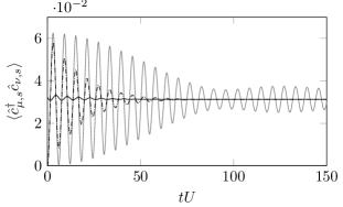
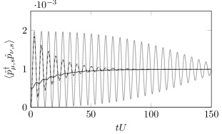
Figure 1: Top: $\langle\hat{c}^{\dagger}_{\mu,s}\hat{c}_{\nu,s}\rangle$-correlations for next neighbours. Bottom: $\langle\hat{p}^{\dagger}_{\mu,s}\hat{p}_{\nu,s}\rangle$-correlations for next but one neighbours. Gray curves: Quench from $J/U=0$ to $J/U=0.4$ with $\gamma=0$, Dashed curves: Quench from $J/U=\gamma/U=0$ to $J/U=0.4$ and $\gamma/U=0.05$, solid black curves: Evolution from the ground state to the prethermalized state after coupling the system to the environment with $\gamma/U=0.05$.

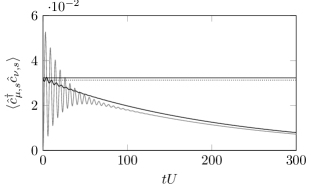
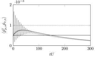
Figure 2: Top: $\langle\hat{c}^{\dagger}_{\mu,s}\hat{c}_{\nu,s}\rangle$-correlations for next neighbours with backreaction. Bottom: $\langle\hat{p}^{\dagger}_{\mu,s}\hat{p}_{\nu,s}\rangle$-correlations for next but one neighbours with backreaction. Gray curves: Quench from $J/U=\gamma/U=0$ to $J/U=0.4$ and $\gamma/U=0.05$, solid black curves: Evolution from the ground state after coupling the system to the environment with $\gamma/U=0.05$. Solid line: Ground state, dotted line: prethermalized state.

Back-reaction

So far, we have neglected the back-reaction of the quantum or thermal fluctuations of the quasi-particles onto the mean field and assumed that $\hat{\rho}_{\mu}^{0}$ and thus the double occupancy $\mathfrak{D}$ are constant. In order to study this back-reaction, we insert the (generally time-dependent) solutions $f^{00}_{\mbox{\boldmath$\scriptstyle k$}}$, $f^{01}_{\mbox{\boldmath$\scriptstyle k$}}$, $f^{10}_{\mbox{\boldmath$\scriptstyle k$}}$, and $f^{11}_{\mbox{\boldmath$\scriptstyle k$}}$ back into into (4) which gives

$$i\partial_{t}{\mathfrak{D}}=\frac{2}{N}\sum\limits_{\mbox{\boldmath$\scriptstyle k$}}J_{\mbox{\boldmath$\scriptstyle k$}}\left(f^{01}_{\mbox{\boldmath$\scriptstyle k$}}-f^{10}_{\mbox{\boldmath$\scriptstyle k$}}\right)\,.$$ (16)

We see that even the asymptotic state (Pre-thermalization) can induce a change of $\mathfrak{D}$ provided that $\gamma\neq 0$. For example, starting in the Mott insulator phase with zero or small $\mathfrak{D}$, it would slowly grow due to local on-site heating induced by the coupling to the environment.

However, this growth rate is much slower than the damping of correlations and quasi-particles with their decay rate $\gamma$. From the above equation (16), we may estimate that this local on-site heating occurs on much longer time scales

$$\tau_{\rm thermal}\sim\frac{U^{2}}{J^{2}}\,\frac{Z}{\gamma}\gg\frac{1}{\gamma}=\tau_{\rm decay}\,,$$ (17)

where the factor of $Z$ stems from the Fourier transform (assuming an isotropic lattice).

For late times $t\gg\tau_{\rm thermal}$, the double occupancy tends to 1/4 and thus all correlations between lattice sites vanish, as we may infer from (Pre-thermalization). This final state $\hat{\rho}_{\mu}\propto\mbox{\boldmath$1$}$ corresponds to the infinite-temperature limit, which is consistent with the fact that the considered Markovian environment acts as an infinite temperature heat bath.

Hubbard Dimer

The previous investigations were based on the hierarchy of correlations, which can be motivated by the formal limit $Z\to\infty$. However, the results obtained via this method (such as the damping of quasi-particles and pre-thermalization) can be applied qualitatively to scenarios beyond this approximation. To see this, let us consider a simple system which admits an exact solution – the Fermi-Hubbard model consisting of two lattice sites (Hubbard dimer) with one spin-up and one spin-down particle.

To simplify the analysis further, we consider states which are fully symmetric with respect to a permutation of the lattice sites $\mu=1$ and $\nu=2$ and are invariant under spin-flips (i.e., unpolarized). Again, the on-site matrices $\hat{\rho}_{1}^{0}=\hat{\rho}_{2}^{0}$ can be fully parametrized by the double occupancy $\mathfrak{D}$ via the ansatz (7). Furthermore, as we only have one particle per spin species, the particle-particle $f^{11}_{12,s}$ and hole-hole $f^{00}_{12,s}$ correlators vanish and only the particle-hole correlators $f^{01}_{12,s}$ and $f^{10}_{12,s}$ remain. Finally, the only remaining non-zero expectation values are two higher-order correlators $\langle\hat{c}_{1\uparrow}^{\dagger}\hat{c}_{1\downarrow}\hat{c}_{2\downarrow}^{\dagger}\hat{c}_{2\uparrow}\rangle$ and $\langle\hat{c}_{1\uparrow}^{\dagger}\hat{c}_{1\downarrow}^{\dagger}\hat{c}_{2\downarrow}\hat{c}_{2\uparrow}\rangle$.

Now, combining these five relevant expectation values (in the mentioned order) into a vector $v$, the time-evolution can be described exactly by a $5\times 5$-matrix

$$i\partial_{t}\mbox{\boldmath$v$} = \left(\begin{array}[]{ccccc}0&-J&J&0&0\\ -4J&-U-i\gamma&0&-2J&J\\ 4J&0&+U-i\gamma&2J&-J\\ 0&-J&J&-2i\gamma&0\\ 0&2J&-2J&0&-4i\gamma\end{array}\right)\cdot\mbox{\boldmath$v$}$$ (24)

$$+\mbox{\boldmath$s$}\,,$$

where $\mbox{\boldmath$s$}=(0,J,-J,0,0)^{\rm T}$ are the source terms already discussed above. This simple matrix equation describes the exact evolution – but, unfortunately, there is no simple closed expression for the eigenvalues and eigenvectors of this matrix. Thus, let us discuss some limiting cases: Without the environment, i.e., for $\gamma=0$, two eigenvalues correspond to the quasi-particle energy $\pm\sqrt{16J^{2}+U^{2}}$ while the other three vanish. In order to include the environment, we consider the strongly interacting regime where $J\ll U$, i.e., deep in the Mott insulator phase. In this regime, one may infer from the diagonal of the above matrix (24) that four eigenvalues have imaginary parts of order $\gamma$, which corresponds to the decay of the four correlation functions to a pre-thermalized state on a time scale of order $1/\gamma$. However, the remaining eigenvalue (which corresponds to the evolution of the double occupancy $\mathfrak{D}$) is much smaller

$$\lambda=-\frac{8i\gamma J^{2}}{U^{2}+\gamma^{2}}+\,{\cal O}\left(\frac{J^{3}}{U^{3}}\right)\Rightarrow|\lambda|\ll\gamma\,.$$ (25)

We see that, while all the correlations approach their pre-thermalized state on a time scale of order $1/\gamma$, full thermalization is governed by the above eigenvalue and thus occurs on much longer times. Again, due to local on-site heating, the state $v$ approaches the final state $\mbox{\boldmath$v$}=(1/4,0,0,0,0)^{\rm T}$, which corresponds to an infinite-temperature state $\hat{\rho}_{12}\propto\mbox{\boldmath$1$}$.

Conlcusions

As a prototypical example for an interacting quantum many-body system, we consider the Fermi-Hubbard model (1) and couple it to a Markovian environment (2) which permanently performs weak measurements of the particle numbers $\hat{n}_{\mu}^{\uparrow}$ and $\hat{n}_{\mu}^{\downarrow}$ for each lattice site $\mu$. Via the hierarchy of correlations, we derive the evolution equations (Quasi-particles) for the correlations, which are linear to first order (in $1/Z$), as well as their back-reaction (16) onto the mean field.

As expected, the coupling $\gamma$ to the environment induces an imaginary part of the eigen-frequencies (10) leading to a decay of the quasi-particles and tends to suppress the correlations. Quite surprisingly, this damping mechanism does also induce the phenomenon of pre-thermalization quite analogous to a quantum quench. For small $\gamma$, the correlations even approach the same pre-thermalized state as after a quench. As our general arguments from (13) to (15) indicate, this seems to be a general phenomena and shows that the environment induced damping of quasi-particles has a very similar effect as the dephasing of quasi-particles after a quench.

Taking the back-reaction (16) into account, we find that the system eventually approaches a thermal state of infinite temperature. However, this on-site heating process is much slower and requires time scales (17) much longer than the intermediate time scale $\,{\cal O}(1/\gamma)$ of pre-thermalization. Finally, in order to test the reliability of our approximation scheme, we considered the exactly solvable case of the two-site Fermi-Hubard model (Hubbard dimer) and found qualitatively the same results. We also considered the Mott-Neel state displaying anti-ferromagnetic spin ordering (see the supplement) and found analogous behavior.

I Hierarchy of Correlations

Up to first order in $1/Z$, the equations of motion for the double occupancy and the two-point-correlations have the explicit form

$$i\partial_{t}\mathfrak{D} =\frac{1}{Z}\sum_{\kappa,s}J_{\mu\kappa}(f^{01}_{\kappa\mu,s}-f^{10}_{\mu\kappa,s})+\mathcal{O}(1/Z^{2})$$ (26)

$$i\partial_{t}f^{ij}_{\mu\nu,s} =\frac{1}{Z}\sum_{\kappa,l}J_{\mu\kappa}\langle\hat{n}^{i}_{\mu,\bar{s}}\rangle f^{lj}_{\kappa\nu,s}-\frac{1}{Z}\sum_{\kappa,l}J_{\nu\kappa}\langle\hat{n}^{j}_{\nu,\bar{s}}\rangle f^{il}_{\mu\kappa,s}$$

$$+\frac{J_{\mu\nu}}{Z}[\langle\hat{n}^{i}_{\mu,\bar{s}}\rangle\langle\hat{n}^{1}_{\nu,s}\hat{n}^{j}_{\nu,\bar{s}}\rangle-\langle\hat{n}^{j}_{\nu,\bar{s}}\rangle\langle\hat{n}^{1}_{\mu,s}\hat{n}^{i}_{\mu,\bar{s}}\rangle]$$

$$-(U^{i}-U^{j}+i\gamma)f^{ij}_{\mu\nu,s}+\mathcal{O}(1/Z^{2})\,,$$ (27)

where we used the shorthand notation $\hat{n}^{1}_{\mu,s}=\hat{n}_{\mu,s}$ and $\hat{n}^{0}_{\mu,s}=1-\hat{n}_{\mu,s}$. After a Fourier transformation of (27) for a spatially homogeneous system at half filling, one obtains the set of equations (9) in the letter.

Since the hierarchical set of equations (27) is derived in real space, we are not restricted to spatially homogeneous systems. For example, the fermionic Hubbard system in a hypercubic lattice prefers to be in a staggered Mott-Néel state with sublattices $A$ and $B$ if the temperature is sufficiently low. Assuming to lowest order a perfect staggering, $\hat{n}^{A}_{s}=\hat{n}^{B}_{\bar{s}}=1$, the Fourier components of the correlation functions satisfy the equations

$$(i\partial_{t}+i\gamma)f^{00,AA}_{\mathbf{k},s} =J_{\mathbf{k}}(f^{10,BA}_{\mathbf{k},s}-f^{01,AB}_{\mathbf{k},s})$$ (28)

$$(i\partial_{t}+i\gamma)f^{11,BB}_{\mathbf{k},s} =J_{\mathbf{k}}(f^{01,AB}_{\mathbf{k},s}-f^{10,BA}_{\mathbf{k},s})$$ (29)

$$(i\partial_{t}-U+i\gamma)f^{01,AB}_{\mathbf{k},s} =J_{\mathbf{k}}(f^{11,BB}_{\mathbf{k},s}-f^{00,AA}_{\mathbf{k},s})-J_{\mathbf{k}}$$ (30)

$$(i\partial_{t}+U+i\gamma)f^{10,BA}_{\mathbf{k},s} =J_{\mathbf{k}}(f^{00,AA}_{\mathbf{k},s}-f^{11,BB}_{\mathbf{k},s})+J_{\mathbf{k}}\,.$$ (31)

After a quantum quench, the correlation functions approach the asymptotic state

$$f^{11,BB}_{\mathbf{k},s} =-f^{00,AA}_{\mathbf{k},s}=\frac{2J_{\mathbf{k}}^{2}}{\gamma^{2}+4J_{\mathbf{k}}^{2}+U^{2}}$$ (32)

$$f^{01,AB}_{\mathbf{k},s} =\left(f^{10,BA}_{\mathbf{k},s}\right)^{*}=\frac{J_{\mathbf{k}}(U+i\gamma)}{\gamma^{2}+4J_{\mathbf{k}}^{2}+U^{2}}$$ (33)

whereas the ground state correlations ($\gamma=0$) have the form

$$f^{11,BB}_{\mathbf{k},s} =-f^{00,AA}_{\mathbf{k},s}=\frac{1}{2}\left(1-\frac{U}{\sqrt{4J_{\mathbf{k}}^{2}+U^{2}}}\right)$$ (34)

$$f^{01,AB}_{\mathbf{k},s} =f^{10,BA}_{\mathbf{k},s}=\frac{J_{\mathbf{k}}}{\sqrt{4J_{\mathbf{k}}^{2}+U^{2}}}\,.$$ (35)

II Hubbard Dimer

In general, the dynamics of spins on two lattice sites can be described with a set of 16 coupled equations. Under the assumption that the state is symmetrix w.r.t. spin- and lattice-permutation, the system reduces to 5 coupled equations. With the definitions

$$\mathfrak{D} =\langle\hat{n}_{1,s}\hat{n}_{1,\bar{s}}\rangle=\langle\hat{n}_{2,s}\hat{n}_{2,\bar{s}}\rangle$$ (36)

$$\mathfrak{F} =\langle\hat{c}^{\dagger}_{1,s}\hat{n}_{1,\bar{s}}\hat{c}_{2,s}(1-\hat{n}_{2,\bar{s}})\rangle+\langle\hat{c}^{\dagger}_{2,s}\hat{n}_{2,\bar{s}}\hat{c}_{1,s}(1-\hat{n}_{1,\bar{s}})\rangle$$ (37)

$$\mathfrak{S} =\langle\hat{c}^{\dagger}_{1,s}\hat{c}_{1,\bar{s}}\hat{c}^{\dagger}_{2,\bar{s}}\hat{c}_{2,s}\rangle$$ (38)

$$\mathfrak{H} =\langle c^{\dagger}_{1\uparrow}c^{\dagger}_{1\downarrow}c_{2\uparrow}c_{2\downarrow}\rangle+\langle c^{\dagger}_{2\uparrow}c^{\dagger}_{2\downarrow}c_{1\uparrow}c_{1\downarrow}\rangle$$ (39)

we can write the dynamics of the Dimer as

$$i\partial_{t}\mathfrak{D} =J(\mathfrak{F}^{*}-\mathfrak{F})$$ (40)

$$(i\partial_{t}+U+i\gamma)\mathfrak{F} =-4J\mathfrak{D}-2J\mathfrak{S}+J\mathfrak{H}+J$$ (41)

$$(i\partial_{t}-U+i\gamma)\mathfrak{F}^{*} =4J\mathfrak{D}+2J\mathfrak{S}-J\mathfrak{H}-J$$ (42)

$$(i\partial_{t}+2i\gamma)\mathfrak{S} =J(\mathfrak{F}^{*}-\mathfrak{F})$$ (43)

$$(i\partial_{t}+4i\gamma)\mathfrak{H} =-2J(\mathfrak{F}^{*}-\mathfrak{F})$$ (44)

For a finite damping rate, the system runs into the infinite temperature state with $\mathfrak{D}=1/4$ and $\mathfrak{F}=\mathfrak{S}=\mathfrak{H}=0$. For $\gamma=0$, the prethermalized state of the system is given by

$$\mathfrak{D}_{\mathrm{asy}} =\mathfrak{S}_{\mathrm{asy}}=-\frac{\mathfrak{H}_{\mathrm{asy}}}{2}=\frac{2J^{2}}{16J^{2}+U^{2}}$$ (45)

$$\mathfrak{F}_{\mathrm{asy}} =\mathfrak{F}^{*}_{\mathrm{asy}}=\frac{JU}{16J^{2}+U^{2}}\,.$$ (46)

The ground state of the system can be determined by an adiabatic increase of the hopping rate to a finite value:

$$\mathfrak{D}_{\mathrm{ground}} =\mathfrak{S}_{\mathrm{ground}}=-\frac{\mathfrak{H}_{\mathrm{ground}}}{2}$$

$$=\frac{1}{8}\left(1-\frac{U}{\sqrt{16J^{2}+U^{2}}}\right)$$ (47)

$$\mathfrak{F}_{\mathrm{ground}} =\mathfrak{F}^{*}_{\mathrm{ground}}=\frac{J}{\sqrt{16J^{2}+U^{2}}}$$ (48)

References

- (1) J. Hubbard, Proc. R. Soc. Lond. A 276, 238 (1963).
- (2) M. Imada, A. Fujimori, and Y. Tokura, Rev. Mod. Phys. 70 (1998).
- (3) P. Calabrese and J. Cardy, Phys. Rev. Lett. 96, 136801 (2006).
- (4) S. R. Manmana, S. Wessel, R. M. Noack, and A. Muramatsu, Phys. Rev. Lett. 98, 210405 (2007).
- (5) A. Iucci and M. A. Cazalilla, Phys. Rev. A 80, 063619 (2009).
- (6) M. Schiró and M. Fabrizio, Phys. Rev. B 83, 165105 (2011).
- (7) M. Moeckel and S. Kehrein, Phys. Rev. Lett. 100, 175702 (2008).
- (8) M. Eckstein, M. Kollar, and P. Werner, Phys. Rev. Lett. 103, 056403 (2009).
- (9) C. Kollath, A. M. L äuchli, and E. Altman, Phys. Rev. Lett. 98, 180601 (2007).
- (10) G. Biroli, C. Kollath, and A. M. Läuchli, Phys. Rev. Lett. 105, 250401 (2010).
- (11) G. Roux, Phys. Rev. A 79, 021608 (2009).
- (12) G. Roux, Phys. Rev. A 81, 053604 (2010).
- (13) M. Cramer, C. M. Dawson, J. Eisert, and T. J. Osborne, Phys. Rev. Lett. 100, 030602 (2008).
- (14) M. Cramer , A. Flesch, I. P. McCulloch, U. Schollw öck, and J. Eisert, Phys. Rev. Lett. 101, 063001 (2008).
- (15) A. Flesch, M. Cramer, I. P. McCulloch, U. Schollwöck, and J. Eisert, Phys. Rev. A 78, 033608 (2008).
- (16) A. M. Läuchli and C. Kollath, J. Stat. Mech.: Theory and Experiment, P05018 (2008).
- (17) J.-S. Bernier, G. Roux, and C. Kollath, Phys. Rev. Lett. 106 200601 (2011).
- (18) J-S. Bernier, D. Poletti, P. Barmettler, G. Roux, and C. Kollath, Phys. Rev. A 85, 033641 (2012).
- (19) P. Barmettler, D. Poletti, M. Cheneau, and C. Kollath, Phys. Rev. A 85, 053625 (2012).
- (20) F. Queisser, K. V. Krutitsky, P. Navez, and R. Schützhold, Phys. Rev. A 89, 033616 (2014).
- (21) K. V. Krutitsky, P. Navez, F. Queisser, and R. Schützhold, EPJ Quant. Tech. 1 12 (2014).
- (22) P. Navez, F. Queisser, and R. Schützhold, Jour. Phys. A: Math. and Theor. 47 225004 (2014).
- (23) F. Queisser, P. Navez, and R. Schützhold, Phys. Rev. A 85, 033625 (2012).
- (24) P. Navez, F. Queisser, and R. Schützhold, Phys. Rev. A 94, 023629 (2016).
- (25) P. Navez and R. Schützhold, Phys. Rev. A 82, 063603 (2010).
- (26) T. Esslinger, Ann. Rev. Cond. Mat. Phys. 1 129 (2010).
- (27) R. Jördens, N. Strohmaier, K. Günter, H. Moritz, and T. Esslinger, Nature 455 204 (2008).
- (28) L. W. Cheuk, M. A. Nichols, K. R. Lawrence, M. Okan, H. Zhang, E. Khatami, N. Trivedi, T. Paiva, M. Rigol, M. W. Zwierlein, Science 353 1260 (2016).
- (29) M. Boll, T. A. Hilker, G. Salomon, A. Omran, J. Nespolo, L. Pollet, I. Bloch, C. Gross, Science 353 1257 (2016).
- (30) M. F. Parsons, A. Mazurenko, C S. Chiu, Ge. Ji, D. Greif, M. Greiner, Science 353 1253 (2016). Experiment Hubbard solid state
- (31) P. A. Lee, N. Nagaosa, and X.-G. Wen Rev. Mod. Phys. 78, 17 (2006).
- (32) A. Damascelli, Z. Hussain, and Z.-X. Shen Rev. Mod. Phys. 75, 473 (2003).
- (33) M. Moeckel and S. Kehrein, Ann. Phys. 324 2146 (2009).
- (34) R. Staudt, M. Dzierzawa, and A. Muramatsu, The European Phys. J. B: Cond. Mat. 17 411 (200).