KDSL: a Knowledge-Driven Supervised Learning Framework for
Word Sense Disambiguation

Abstract

We propose KDSL, a new word sense disambiguation (WSD) framework that utilizes knowledge to automatically generate sense-labeled data for supervised learning. First, from WordNet, we automatically construct a semantic knowledge base called DisDict, which provides refined feature words that highlight the differences among word senses, i.e., synsets. Second, we automatically generate new sense-labeled data by DisDict from unlabeled corpora. Third, these generated data, together with manually labeled data and unlabeled data, are fed to a neural framework conducting supervised and unsupervised learning jointly to model the semantic relations among synsets, feature words and their contexts. The experimental results show that KDSL outperforms several representative state-of-the-art methods on various major benchmarks. Interestingly, it performs relatively well even when manually labeled data is unavailable, thus provides a potential solution for similar tasks in a lack of manual annotations.

1 Introduction

Word sense disambiguation (WSD) is the task to identify the sense of a word under certain context. It is one of the central tasks for understanding natural languages. WSD has been widely used in many basic natural language processing (NLP) tasks or downstream applications, such as sentiment analysis (Huang et al., 2012) and machine translation (Neale et al., 2016).

Approaches for WSD are divided into two groups, i.e., (semi) supervised learning (Lee and Ng, 2002; Zhi and Ng, 2010; Kågebäck and Salomonsson, 2016; Iacobacci, Pilehvar, and Navigli, 2016; Yuan et al., 2016; Melamud, Goldberger, and Dagan, 2016; Raganato, Bovi, and Navigli, 2017) and knowledge-based approaches (Lesk, 1986; Banerjee and Pedersen, 2003; Agirre and Soroa, 2009; Miller et al., 2012; Moro, Raganato, and Navigli, 2014; Basile, Caputo, and Semeraro, 2014a). In general, the former approaches perform better than the latter in most benchmarks. However, most supervised learning approaches for WSD are heavily dependent on the amount of sense-labeled data. Unfortunately, sense-labeled data is far from adequate for supervised systems to perform well due to the high cost of manual annotations. For synsets never occurred in the training corpora, these methods can not learn to make plausible predictions.

Motivated by this, we propose KDSL, a new framework to combine supervised learning and knowledge-based approaches for WSD by automatically generating sense-labeled data from explicit knowledge bases as the training dataset for supervised learning. More precisely, we first build a high quality semantic knowledge base from WordNet (Miller, 1995) that highlights the differences among word senses. Then, we utilize this knowledge base to generate sense-labeled data from raw sentences. Finally, these automatically generated data are fed to a neural network to model the semantic relationships among word senses, feature words and their contexts.

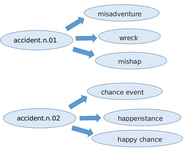
(a) Two synsets of the word “accident” in DisDict

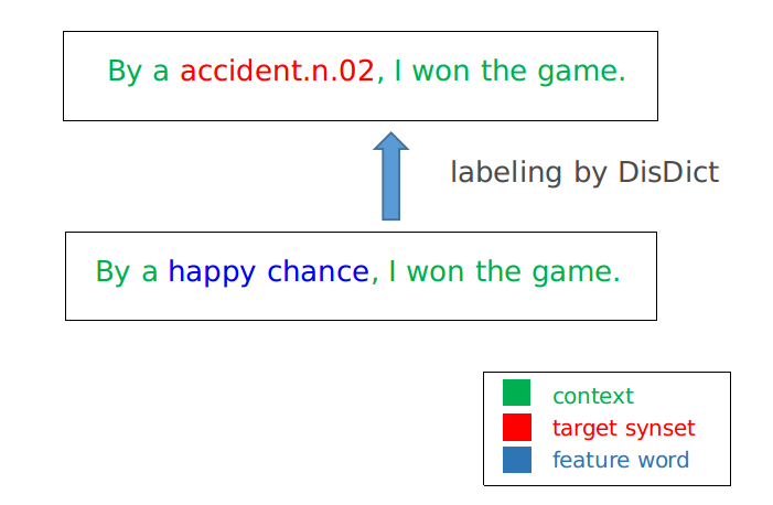
(b) Since “happy chance” serves as a feature word for “accident.n.02”, labeling the context of “happy chance”
with “accident.n.02” as a new supervised learning instance

Figure 1: Generating labeled data for “accident.n.02” by DisDict from plain sentences

For the first step, we construct DisDict, a semantic KB customized for WSD, which is automatically extracted from WordNet by a statistic model. It selects simple feature words to highlight the differences among word senses, i.e., synsets. DisDict contains a number of triples of the form (synset, feature words, confidence score) for all synsets in WordNet 3.0, which contains a total number of 117659 synsets covering nouns, verbs, adjectives and adverbs. The feature words are selected based on two criteria. Firstly, they should have similar semantics with the synset. Secondly, different from previous semantic KBs such as WordNet and ConceptNet, DisDict specifically aims at WSD, i.e., to highlight the differences among different synsets during knowledge extraction. For instance, depicted in Figure 1, the word “accident” has two synsets, namely “accident.n.01” for “an unfortunate mishap; especially one causing damage or injury”, and “accident.n.02” for “anything that happens suddenly or by chance without an apparent cause”. For the synset “accident.n.01”, DisDict chooses “misadventure”, “wreck”, “mishap” as the feature words with highest confidence scores, while for “accident.n.02”, the top three feature words are “chance event”, “happenstance” and “happy chance”. Clearly, those two sets of feature words provide significant discriminative information between these two synsets.

The second step is to generate sense-labeled data automatically by DisDict from raw sentences. Since a synset is semantically similar to its feature words in DisDict, if one of these words occurs in a sentence, we label the context with the synset as a new instance. For instance, depicted in Figure 1, since “happy chance” serves as a feature word for “accident.n.02”, the context in which “happy chance” occurs is labeled with “accident.n.02” and can be fed into supervised learning. In this way, we can generate much new labeled data for target synsets.

The final step is to design a neural framework conducting learning on these generated data, together with manually labeled data and unlabeled data. Depicted in Figure 2, given a sentence and a word in it to be disambiguated, the neural network takes the left context before the word and the right context after the word as the input, and uses a binary long short-term memory (BLSTM) encoder to encode them as a fixed-length context embedding, which is fed into a fully connected network with multi softmax outputs for predictions. As a supervised learning task, this encoder is trained jointly on data automatically generated by DisDict as well as data manually labeled to predict the proper synsets by their contexts. We set a param to control the ratio of samples from the two data sources. To improve the generalization ability, we also design an unsupervised learning task, i.e., training the encoder on unlabeled corpora to predict words by their left and right contexts, as depicted in Figure 2.

We conduct empirical evaluations on various major WSD datasets and our method outperforms a number of representative approaches. Experiments show that incorporating supervised learning on the data generated by DisDict improves the performance for WSD. Even when there is no sense-labeled data, our work also performs well and beats MFS, which is a state-of-the-art knowledge-based WSD method. Our approach illustrates that the combination of semantic knowledge and unlabeled data is useful to generate high quality sense-labeled data and provides a potential solution for similar tasks without manually labeled data.

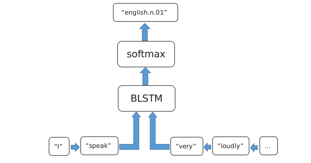
(a) Supervised learning to predict synset “english.n.01” by the left context “I speak” and right context “very loudly …” of “English” in sense-labeled corpora

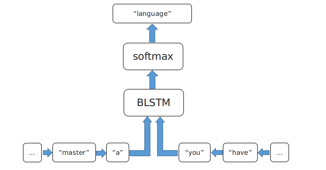
(b) Unsupervised learning to predict word “language” by its left context “To master a” and right context “you have to practice listening and speaking …” in unlabeled corpora

Figure 2: Supervised and unsupervised learning for WSD

2 Related Work

In this section, we will briefly review previous approaches about supervised WSD, knowledge-based WSD, combined methods and data generation strategies for this task.

2.1 Supervised WSD

Supervised WSD is trained on sense-labeled corpora. The labels and features for training are extracted either manually or automatically. Zhi and Ng (2010) utilized surrounding words, POS tags of surrounding words and local collocations as features and trained a classifier for WSD. Rothe and Schütze (2015) leveraged WordNet to generate synset embeddings from word embeddings and convert them into features of a supervised learning system. Kågebäck and Salomonsson (2016) proposed an approach based on bidirectional LSTM to model sequence of words surrounding the target word without hand-crafted features. Iacobacci, Pilehvar, and Navigli (2016) published a full evaluation study on equipping supervised WSD with word embeddings. To alleviate the lack of sufficient manually labeled corpora, Yuan et al. (2016) proposed a semi-supervised framework with label propagation to expand training corpora. Melamud, Goldberger, and Dagan (2016) proposed a generic model for representation of context, i.e., context2vec, and fed it into a classifier for WSD. Uslu et al. (2018) proposes fastsense, a neural WSD model with high learning efficiency.

2.2 Knowledge-based WSD

Knowledge-based approaches rely on manually constructed human knowledge base. Lesk (1986) proposed definition (gloss) overlap measure, i.e., to calculate overlaps among the definitions of the target word and those surrounding it in the given context to determine word sense. It was enhanced by Banerjee and Pedersen (2003) to take definitions of related words into consideration. Chen and Liu (2011) combined both WordNet and ConceptNet to judge word sense. Taking advantages of distributional similarity (Miller et al., 2012; Basile, Caputo, and Semeraro, 2014b; Chen, Liu, and Sun, 2014; Camacho-Collados et al., 2016) has also been shown effective. Agirre and Soroa (2009); Guo and Diab (2010); Agirre, de Lacalle, and Soroa (2014); Moro, Raganato, and Navigli (2014); Weissenborn et al. (2015); Tripodi and Pelillo (2017) modeled knowledge bases as graphs, i.e., words as nodes and relations as edges. The senses preferences of each word are updated iteratively according to certain graph-based algorithms. Pasini and Navigli (2018) proposed two knowledge-based methods for learning the distribution of senses.

2.3 Combined methods and data generation strategies

Rothe and Schütze (2015) leveraged WordNet to generate synset embeddings from word embeddings and convert them into features of a supervised learning system; Raganato, Bovi, and Navigli (2017) introduced several advanced neural sequence learning models to WSD and design a multi-task mechanism to predict synsets as well as their coarse-grained semantic labels. Taghipour and Ng (2015) proposed OMSTI, a sense-labeled corpus generated through the disambiguation of a multilingual parallel corpus; Pasini and Navigli (2017) proposed Train-O-Matic, a data generation strategy based on random walk in WordNet.

3 Models

3.1 Problem Formalization

Suppose there is a sentence $c$ with words in order: $w_{1}$, $w_{2}$, …, $w_{L}$, each of which is tagged with its POS. For instance, in a sentence “Knowledge is power”, $w_{1}$=“knowledge_NOUN”, where the suffix “_NOUN” means its POS is noun. For each $w_{i}$ in $c$, there is a set of candidate synsets $CS(w_{i})=\{s_{1}(w_{i}),s_{2}(w_{i}),...,s_{K}(w_{i})\}$. If two synsets are both candidate synsets for a certain word, it is called that they have competitive relations in this paper. The goal of word sense disambiguation (WSD) is to identify the correct synset of $w_{i}$ given the context $c$. For a corpus $T$ with sentences $c_{1}$, $c_{2}$, …, $c_{N}$, the collection of all target words to be disambiguated in $T$ is denoted as $TW$, the collection of all candidate synsets for words in $TW$ is denoted as $TS$. And in DisDict, there are several feature words to interpret the semantics of each synset, the collection of all feature words is denoted as $FW=\cup_{i}FW(s_{i})$, while $FW(s_{i})$ is the collection of feature words of synset $s_{i}$.

3.2 Knowledge Base for WSD: DisDict

Motivations

For our work, we need a semantic KB to generate sense-labeled data. However, existing semantic KBs are hard to use directly. There are two main disadvantages:

a) Coarse-grained. Some semantic KBs, e.g., ConceptNet, only provide word (or phrase) level knowledge and do not distinguish different potential senses of a given word (phrase) explicitly;

b) (Partially) unstructured. WordNet and BabelNet (Navigli and Ponzetto, 2012) provide glosses of synsets by unstructured texts which are hard to encode and utilize by neural models.

Motivated by these disadvantages, we propose DisDict, a semantic KB aiming at WSD. The ideas for DisDict are also also twofold:

a) Establishing synset level semantic knowledge;

b) Extracting high-quality semantic information from (partially) unstructured knowledge to highlight the distinction among candidate synsets. In DisDict, only words having high statistic correlations with the target synset are selected as its feature words. These words are tagged with confidence scores by a statistic model. Noisy words or words with little discriminative information for synsets are removed.

(player.n.01, playmaker, 0.11)	(arrive.v.01, flood in, 0.21)
(player.n.01, seeded player, 0.11)	(arrive.v.01, plump in, 0.21)	(brainy.s.01, brainy, 0.52)
(player.n.01, dart player, 0.11)	(arrive.v.01, drive in, 0.16)
(player.n.01, most valuable player, 0.11)	(arrive.v.01, move in, 0.16)	(brainy.s.01, smart as a whip, 0.36)
(player.n.01, volleyball player, 0.11)	(arrive.v.01, get in, 0.05)
(player.n.01, pool player, 0.09)	(arrive.v.01, come in, 0.04)	(brainy.s.01, impressive, 0.06)
(player.n.01, lacrosse player, 0.09)	(arrive.v.01, draw in, 0.04)
(player.n.01, grandmaster, 0.09)	(arrive.v.01, set down, 0.04)	(brainy.s.01, unusual, 0.05)
(player.n.01, scorer, 0.09)	(arrive.v.01, roll up, 0.04)
(player.n.01, billiard player, 0.09)	(arrive.v.01, attain, 0.03)
(musician.n.01, flutist, 0.1)
(musician.n.01, vibist, 0.1)	(arrive.v.02, succeed, 0.41)
(musician.n.01, accompanist, 0.1)		(brilliant.s.01, transcendent, 0.57)
(musician.n.01, harmonizer, 0.1)
(musician.n.01, gambist, 0.1)	(arrive.v.02, come through, 0.4)
(musician.n.01, carillonneur, 0.1)		(brilliant.s.01, surpassing,0.43)
(musician.n.01, recorder player, 0.1)
(musician.n.01, harper, 0.1)	(arrive.v.02, win, 0.2)
(musician.n.01, keyboardist, 0.1)
(musician.n.01, accompanyist, 0.1)

Table 1: A glance of DisDict

Construction of DisDict

To build DisDict, firstly, words from Synonymy, Hypernymy/Hyponymy and Gloss in WordNet are harvested as potential feature words. A word in a synset’s gloss is likely to be its feature word only if it has the same POS with the synset. For instance, since the gloss of synset “english.n.01” is “the people of England”, then “people” and “England” are considered as potential feature words of “english.n.01”.

Then a statistic model is implemented to select words having high statistical correlations with the synsets from potential feature words. This model is similar to PMI (point-wise mutual information) and was firstly proposed by Wettler (1993) to compute word associations. For each (synset, feature word) pair ($s_{i}$, $w_{j}$), $r_{ij}$ represents the strength of their correlations:

$$r_{ij}=\frac{p(s_{i},w_{j})}{p(s_{i})p(w_{j})^{\tau}}=\frac{p(s_{i},w_{j})}{\sum_{w}{p(s_{i},w)}\sum_{s}{p(s,w_{j})}^{\tau}}$$ (1)

where $p(s_{i},w_{j})$ is the co-occurrence probability, which is proportional to the times $s_{i}$ associated with $w_{j}$ in WordNet. For instance, when traversing WordNet, if $w_{j}$ occurs twice in the gloss of $s_{i}$, then $p(s_{i},w_{j})\leftarrow p(s_{i},w_{j})+2$. $\tau$ is an adjustable parameter to control the effect of word frequencies. For each target synset $s_{i}$, only a small number ($<=N_{f}$) of feature words with the highest $r_{ij}$ are preserved, others are dropped out. Confidence scores for these $N_{f}$ feature words are normalized such that their sum is 1.0， which is:

$$\begin{split}r_{ij}\leftarrow\frac{r_{ij}}{\sum_{w_{j^{\prime}}\in FW(s_{i})}r_{ij^{\prime}}},w_{j}\in FW(s_{i})\end{split}$$ (2)

DisDict is organized as a number of triples, i.e., $(s_{i},w_{j},r_{ij})$. Table 1 provides a glance of DisDict, i.e., three competitive synsets pairs in DisDict ($N_{f}=10$), i.e., “player.n.01” (“ a person who participates in or is skilled at some game”) and “musician.n.01” (“someone who plays a musical instrument (as a profession)”); “arrive.v.01” (“make a prediction about; tell in advance”) and “arrive.v.02” (“succeed in a big way; get to the top”); “brainy.s.01” (“having or marked by unusual and impressive intelligence”) and “brilliant.s.02” (“of surpassing excellence”). Synsets in the same column have competitive relations with each other.

Sense-Labeled Data Generation by DisDict

The second step is to generate sense-labeled data automatically by DisDict from raw sentences. Since in DisDict a synset is semantically similar to its feature words, if one of them occurs in a sentence, label the sentence with the synset as a new instance. Depicted in Figure 1, since “happy chance” serves as a feature word for “accident.n.02”, the context in which “happy chance” occurs is labeled with “accident.n.02” and can be fed into supervised learning. In this way, we can generate much new labeled data for target synsets.

Synsets in corpora follow a certain frequency distribution. Different synsets may have different frequencies. Since we do not know this distribution a priori, we can only design a model to simulate it, i.e., the frequencies for synset $s_{i}$ are approximately calculated as:

$$\begin{split}f(s_{i})\propto\sum_{w_{j},s_{i}\in CS(w_{j})}f(w_{j})\cdot p^{l_{ij}}\end{split}$$ (3)

where $w_{j}$ is a word of which $s_{i}$ is one of the candidate synsets, i.e., $s_{i}\in CS(w_{j})$; $l_{ij}$ denotes the ranking of $s_{i}$ among synsets in $CS(w_{j})$, e.g., the ranking of “english.n.01” is 1 among the candidate synsets of ”English_Noun” in WordNet; $f(w_{j})$ is the frequency of $w_{j}$ which is counted in a large corpus; $p$ is an adjustable param to control the bias towards synsets with high rankings.

The instances for $s_{i}$ are generated by its feature words, i.e., $FW(s_{i})$. The number of instances contributed by $w_{k}\in FW(s_{i})$ for $s_{i}$, denoted as $f(s_{i},w_{k})$, is set as:

$$\begin{split}f(s_{i},w_{k})=f(s_{i})\cdot r_{ik},w_{k}\in FW(s_{i})\end{split}$$ (4)

3.3 Learning Framework

The learning process has two parts:

a) Supervised Learning: training a model to predict synsets by contexts in sense-labeled corpora. As shown in Figure 2, suppose there is a sentence “I speak English very loudly…” where the word “English” is to be disambiguated. The model is trained to make prediction of “english.n.01” over all synsets given the left (“I speak”) and right (“very loudly …”) context of “English”.

b) Unsupervised learning: training the model in a) to predict words by contexts in large unlabeled corpora. As shown in Figure 2, suppose there is a sentence “To master a language, you have to practice listening and speaking …” where the word “language” is one of the feature words in DisDict, the model is trained to make prediction of “language” given its left (“To master a”) and right (“you have to practice listening and speaking ….”) context. This training process promotes the ability to model context and extract semantic features, which improves the generalization performance.

During training, instances are sampled from manually labeled data and data generated by DisDict. We set a param to control the ratio of samples from the two data sources.

Methods	Test Datasets				Concatenation of All Test Sets
	SE2	SE3	SE13	SE15	Nouns	Verbs	Adj.	Adv.	All
IMS	70.9	69.3	65.3	69.5	70.5	55.8	75.6	82.9	68.9
IMS-s+emb	72.2	70.4	65.9	71.5	71.9	56.6	75.9	84.7	70.1
Context2vec	71.8	69.1	65.6	71.9	71.2	57.4	75.2	82.7	69.6
Le et al. (2017)	70.0	-	66.6	-	-	-	-	-	-
Raganato et al. (2017)	72.0	69.4	66.4	70.8	71.6	57.1	75.6	83.2	69.9
Ours
MLab	69.2	68.3	66.1	67.4	69.4	54.6	75.7	82.4	68.0
MLab+ULab	70.2	69.9	69.3	72.9	72.3	56.8	77.4	81.1	70.4
MLab+ULab+MFS	70.8	69.9	69.8	73.0	72.8	56.8	77.3	81.2	70.7
MLab+DisDict+ULab	72.0	70.5	70.9	72.7	74.3	55.6	77.7	82.4	71.4
MLab+DisDict+ULab+MFS	72.0	71.2	70.9	72.9	74.4	56.0	78.3	82.1	71.7

Table 2: F1-scores (%) for English all-words fine-grained WSD with the utilization of manually labeled training data

3.4 Neural Model

LSTM (Hochreiter and Schmidhuber, 1997; Graves and Schmidhuber, 2005) is a gated type of recurrent neural network (RNN), which is a powerful model for NLP. We follow to choose BLSTM (Graves and Schmidhuber, 2005) as our basic neural encoder. As shown in Figure 1, suppose in a sentence $c$ with words $w_{1},w_{2},...,w_{t},w_{t+1},...,w_{N}$, $w_{t}$ is the target word to be disambiguated. We arrange words surrounding $w_{t}$ in order, which are denoted as $left\_word=[w_{t-T},w_{t-T+1},...,w_{t-1}]$ and $right\_word=[w_{t+1},w_{t+2},...,w_{t+T}]$, where $T$ is the maximal distance we consider. Then the two groups of word sequences are fed into a BLSTM structure with two LSTMs in different directions. The words on the left side of the target word are fed into a left-to-right LSTM while those on the right side of target are fed into right-to-left LSTM. The left-to-right LSTM generates a sequence of hidden state vectors $[\overrightarrow{h_{1}},...,\overrightarrow{h_{T}}]$ and the right-to-left LSTM generates a sequence of hidden state vectors $[\overleftarrow{h_{1}},...,\overleftarrow{h_{T}}]$. Then we get two feature vectors $\overrightarrow{h_{l}}$ and $\overleftarrow{h_{r}}$ for left and right context of $w_{t}$:

$$\overrightarrow{h_{l}}=\overrightarrow{h_{T}},\overleftarrow{h_{r}}=\overleftarrow{h_{T}}$$ (5)

Since the left and right contexts of $w_{t}$ do not contain $w_{t}$ itself, they are denoted as $c\backslash\{w_{t}\}$. The vector representation for context $c\backslash\{w_{t}\}$, i.e., $\overrightarrow{c_{\backslash t}}$, is calculated by a fully connected module which takes the concatenation of $\overrightarrow{h_{l}}$ and $\overleftarrow{h_{r}}$ as input:

$$\begin{split}\overrightarrow{c_{\backslash t}}=&Relu(W_{2}\cdot Relu(W_{1}\cdot[\overrightarrow{h_{l}}:\overleftarrow{h_{r}}]+b_{1})+b_{2})\end{split}$$ (6)

Let $SW$ be all synsets occurred in the training corpora. Let $s_{t}$ be the correct synset for $w_{t}$, the probability distribution $p(s_{t}|{c\backslash\{w_{t}\}})$ over all the synsets $s_{i}\in SW$ is calculated by a softmax layer:

$$p(s_{t}|c\backslash\{w_{t}\})=\frac{exp(\overrightarrow{s_{t}}^{\mathrm{T}}\cdot\overrightarrow{c_{\backslash t}})}{\sum\limits_{s_{i}\in SW}exp(\overrightarrow{s_{i}}^{\mathrm{T}}\cdot\overrightarrow{c_{\backslash t}})}$$ (7)

For a word $w$ in context $c$, the probability distribution $p(w|c\backslash\{w\})$ over all words $w^{\prime}$ is calculated by another softmax layer:

$$p(w|c\backslash\{w\})=\frac{exp(\overrightarrow{w}^{\mathrm{T}}\cdot\overrightarrow{c_{\backslash t}})}{\sum\limits_{w^{\prime}}exp(\overrightarrow{w^{\prime}}^{\mathrm{T}}\cdot\overrightarrow{c_{\backslash t}})}$$ (8)

In the labeled corpus $T=\{c_{1},c_{2},...,c_{N}\}$, for each sentence $c_{j}\in T$, the training objective is:

$$J_{a}=-\sum_{c_{j}}(log(p(s_{t}|c_{j}\backslash\{w_{t}\})))$$ (9)

The training process for (9) is illustrated in Figure 2.

As an unsupervised task, in the unlabeled corpus, the model is trained to make prediction of word $w$ from context $c_{j}\backslash\{w\}$. The objective is illustrated as Figure 2 and formulated by:

$$\begin{split}J_{u}=-\sum_{c_{j}}\sum_{w\in c_{j}\cap FW}(log(p(w|c_{j}\backslash\{w\})))\end{split}$$ (10)

where $\theta$ is an adjustable parameter. The final objective $J$ is the weighted aggregation of $J_{a}$ and $J_{u}$:

$$J=J_{a}+\alpha J_{u}$$ (11)

where $\alpha$ is an adjustable parameter. $J$ is trained to be minimized and equation (7) and (8) are approximated by sampled softmax (Jean et al., 2015) during training. During inferencing, for $w_{t}$ in $c_{j}$ to be disambiguated, the model chooses the candidate synset with highest probability conditioned on $c_{j}$ as output ($s_{o}$), which is formulated by:

$$s_{o}=\arg\max_{s_{t}}(p(s_{t}|c_{j}\backslash\{w_{t}\})),s_{t}\in S(w_{t})$$ (12)

where $S(w_{t})$ is the set of candidate synsets for $w_{t}$, $p(s_{t}|c_{j}\backslash\{w_{t}\})$ is the outputs of our BLSTM encoder.

4 Experiments

4.1 Setup

Baseline Methods: The baselines include some state-of-the-art approaches, i.e., MFS (to directly output the Most Frequent Sense in WordNet); IMS (Zhi and Ng, 2010), a classifier working on several hand-crafted features, i.e., POS, surrounding words and local collocations; Babelfy (Moro, Raganato, and Navigli, 2014), a state-of-the-art knowledge-based WSD system exploiting random walks to connect synsets and text fragments; Lesk_ext+emb (Basile, Caputo, and Semeraro, 2014a), an extension of Lesk by incorporating similarity information of definitions; UKB_gloss (Agirre and Soroa, 2009; Agirre, de Lacalle, and Soroa, 2014), another graph-based method for WSD; A joint learning model for WSD and entity linking (EL) utilizing semantic resources by Weissenborn et al. (2015); IMS-s+emb (Iacobacci, Pilehvar, and Navigli, 2016), the combination of original IMS and word embeddings through exponential decay while surrounding words are removed from features; Context2vec (Melamud, Goldberger, and Dagan, 2016), a generic model for generating representation of context for WSD; Jointly training LSTM with labeled and unlabeled data (Le, Postma, and Urbani, 2017) (this is an open implementation for part of the work of Yuan et al. (2016). Since the models and 100 billion data used in Yuan et al.’s paper are not available, we select Le et al.’s work as an alternative. Le et al.’s work uses 1 billion unlabeled data, which is roughly equal to the size of unlabeled corpus in our work. This makes the comparison more fair); A model jointly learns to predict word senses, POS and coarse-grained semantic labels by Raganato, Bovi, and Navigli (2017); Train-O-Matic (Pasini and Navigli, 2017), a language-independent approach for generating sense-labeled data automatically based on random walk in WordNet and training a classifier on it.

Methods	Concatenation of All Test Sets
MFS	65.8
Babelfy	66.4
UKB_gloss	61.1
Lesk_ext+emb	64.2
Ours
DisDict	66.2
DisDict+MFS	67.2

Table 3: F1-scores (%) for English all-words fine-grained WSD in the absence
of manually labeled training data

Methods	Test Datasets
	SE2	SE3	SE13	SE15
MFS	72.0	72.0	63.0	66.3
OMSTI	73.3	67.5	62.5	63.4
Train-O-Matic	71.1	67.8	65.8	68.1
Weissenborn et al. (2015)	-	68.8	72.8	71.5
Ours
DisDict	73.2	69.0	66.2	70.1
DisDict+MFS	74.6	72.0	65.3	71.0
MLab+DisDict+ULab+MFS	78.0	76.0	70.9	75.1

Table 4: F1-scores (%) for nouns disambiguation

Datasets: We choose Semcor 3.0 (Miller et al., 1994) (226,036 manual sense annotations), which is also used by baselines, as the manually labeled data. We also extract 27,616,880 word-context pairs from Wikipedia April 2010 dump with 1 billion tokens which was preprocessed and utilized by Sun et al. (2016). From which, we generate 11,925,166 sense labeled instances by DisDict. The trained models are evaluated on the fine-grained English all-words WSD task under the standardized evaluation framework released by Navigli, Camacho-Collados, and Raganato (2017). We tune parameters on SemEval-07 task 17 (Pradhan et al., 2007) and test models on four datasets, i.e., senseval-2 (Edmonds and Cotton, 2001) with 2282 synset annotations, senseval-3 task 1 (Snyder and Palmer, 2004) with 1850 annotations, SemEval-13 task 12 (Navigli, Jurgens, and Vannella, 2013) with 1644 annotations and SemEval-15 task 13 (Moro and Navigli, 2015) with 1022 annotations. The word embeddings we use are pretrained on 2 billion ukWac (Baroni et al., 2009) corpus, the same corpus as that used in baseline methods.

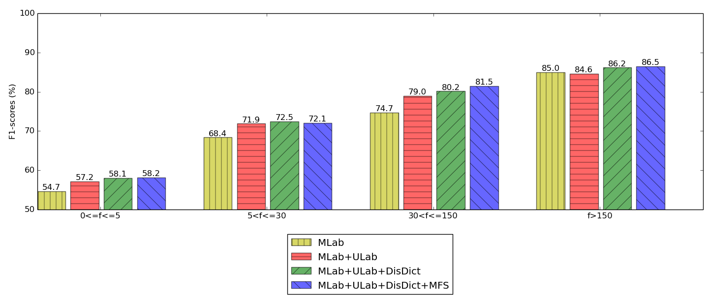
Figure 3: F1-scores (%) for test synsets grouped by their frequencies (f) in the manually
labeled training corpus

Settings: We design a series of experiments based on the combination of four basic settings, i.e., MLab (conducting supervised learning on manually labeled data); ULab (conducting unsupervised on unlabeled data); DisDict (conducting supervised learning on data generated by DisDict); MFS (adding a bias towards the output score of most frequent synset when inferencing). For MLab, if with MFS, we select it as the backoff strategy when the target word is unseen in the training corpora; elsewise, we randomly select a candidate synset to output under such circumstance. For the combination of MLab and DisDict, during training, we sample instances from the two datasets with a ratio to control the balance.

For data generation, $N_{f}$ is set as $10$, $\tau$ in (1) is set as 0.66 and $p$ is set as 0.3 in (3); For training, the BLSTM has 2 layers and 400 hidden units for each individual LSTM; the learning rate for $J$ in (11) is set as $0.1$ and $\alpha$ is $5.0$, we use Mini-batch Gradient Descent to optimize $J$, and the batch size is 80; we apply Dropout (Srivastava et al., 2014) with a rate of 0.5 to prevent over-fitting; the dimension of word and synset embedding is 400; the ratio of samples from manually labeled data and that generated by DisDict is set as $1.0:0.3$; During inferencing, for $MFS$, the bias added to the most frequent synset is set as 0.5.

4.2 Results and Analysis

Table 2 posts the results for English all-words fine-grained WSD with the utilization of manually labeled training data. From the comparison between MLab and MLab+ULab setting, it shows that unsupervised learning improves the generalization performance. From the comparison between MLab+ULab and MLab+DisDict+ULab setting, it illustrates the knowledge in DisDict has a good quality and the combination of knowledge and unlabeled data really generates reliable sense-labeled data, thus improves the overall performance. From the comparison between MLab+DisDict+ULab and MLab+DisDict+ULab+MFS setting, it shows that MFS has a good complementarity to supervised WSD.

Table 3 reports the results of WSD in the absence of manually labeled training data. For fairness, in Table 3, we only make comparison with methods do not need manually labeled data. As shown in Table 3, when there is no manually-labeled data, the combination of our model and MFS, i.e., DisDict+MFS, has outperformed the MFS and Babelfy baseline, thus provides a potential solution for similar tasks in a lack of manual annotations.

Table 4 reports the results of nouns disambiguation on several test sets. Among these settings, MFS, OMSTI, Train-O-Matic, DisDict and DisDict+MFS do not require manually labeled data while Weissenborn et al. (2015) and MLab+DisDict+ULab+MFS require. For data generation methods which are closet to ours, i.e., OMSTI and Train-O-Matic, we train our supervised model on their generated data and post the results. Compared them with DisDict, we can concludes that our new data generation method beats these two approaches by two points. First, these methods only focus on nouns disambiguation, while our work is appropriate to any POS in English. Second, our generated data has a higher quality with a better overall performance on nouns disambiguation.

For fine-grained analysis, we divide synsets in the test sets into four groups according to their frequencies $f$ in the manually labeled training corpus, i.e., $0<=f<=5$, $5<f<=30$, $30<f<=150$, $f>150$, and calculate F1-scores for these groups, as shown in Figure 3. It shows that incorporating data generated by DisDict is beneficial consistently to synsets in each frequency interval from the comparison between MLab+ULab and MLab+DisDict+ULab.

5 Conclusion and Future Work

In this paper, we propose a new framework to combine supervised learning and knowledge-based approaches for word sense disambiguation (WSD). Under this framework, we automatically construct a semantic KB, i.e., DisDict, to highlight the semantic differences among synsets, and utilize DisDict to generate reliable sense-labeled data from unlabeled corpora. Then we apply a neural model to conduct both supervised and unsupervised learning for WSD. Evident from the experiments, our framework outperforms a number of representative approaches on major standard evaluation datasets. Furthermore, our model also achieves better performance against other methods when there is no manually labeled data, thus provides a potential solution for such learning tasks in a lack of manually annotations.

For future work, we will focus on two research lines. First, we will study more powerful approaches to acquire knowledge from unstructured data automatically. Second, we will study a better combination of the data manually labeled and that generated by DisDict.

References

- Agirre and Soroa (2009) Agirre, E., and Soroa, A. 2009. Personalizing pagerank for word sense disambiguation. In EACL 2009, 33–41.
- Agirre, de Lacalle, and Soroa (2014) Agirre, E.; de Lacalle, O. L.; and Soroa, A. 2014. Random walks for knowledge-based word sense disambiguation. Computational Linguistics 40(1):57–84.
- Banerjee and Pedersen (2003) Banerjee, S., and Pedersen, T. 2003. Extended gloss overlaps as a measure of semantic relatedness. In IJCAI 2003, 805–810.
- Baroni et al. (2009) Baroni, M.; Bernardini, S.; Ferraresi, A.; and Zanchetta, E. 2009. The wacky wide web: a collection of very large linguistically processed web-crawled corpora. Language Resources and Evaluation 43(3):209–226.
- Basile, Caputo, and Semeraro (2014a) Basile, P.; Caputo, A.; and Semeraro, G. 2014a. An enhanced lesk word sense disambiguation algorithm through a distributional semantic model. In COLING 2014.
- Basile, Caputo, and Semeraro (2014b) Basile, P.; Caputo, A.; and Semeraro, G. 2014b. An enhanced lesk word sense disambiguation algorithm through a distributional semantic model. In CONLL 2014, 1591–1600.
- Camacho-Collados et al. (2016) Camacho-Collados, J.; Bovi, C. D.; Raganato, A.; and Navigli, R. 2016. A large-scale multilingual disambiguation of glosses. In LREC 2016.
- Chen and Liu (2011) Chen, J., and Liu, J. 2011. Combining conceptnet and wordnet for word sense disambiguation. In IJCNLP 2011.
- Chen, Liu, and Sun (2014) Chen, X.; Liu, Z.; and Sun, M. 2014. A unified model for word sense representation and disambiguation. In EMNLP 2014, 1025–1035.
- Edmonds and Cotton (2001) Edmonds, P., and Cotton, S. 2001. SENSEVAL-2: Overview. In Proceedings of SENSEVAL-2 Second International Workshop on Evaluating Word Sense Disambiguation Systems, 1–5.
- Graves and Schmidhuber (2005) Graves, A., and Schmidhuber, J. 2005. Framewise phoneme classification with bidirectional LSTM and other neural network architectures. Neural Networks 18(5-6):602–610.
- Guo and Diab (2010) Guo, W., and Diab, M. T. 2010. Combining orthogonal monolingual and multilingual sources of evidence for all words WSD. In Proceedings of ACL 2010, 1542–1551.
- Hochreiter and Schmidhuber (1997) Hochreiter, S., and Schmidhuber, J. 1997. Long short-term memory. Neural Computation 9(8):1735–1780.
- Huang et al. (2012) Huang, E. H.; Socher, R.; Manning, C. D.; and Ng, A. Y. 2012. Improving word representations via global context and multiple word prototypes. In ACL 2012: Long Papers-Volume 1, 873–882.
- Iacobacci, Pilehvar, and Navigli (2016) Iacobacci, I.; Pilehvar, M. T.; and Navigli, R. 2016. Embeddings for word sense disambiguation: An evaluation study. In ACL 2016.
- Jean et al. (2015) Jean, S.; Cho, K.; Memisevic, R.; and Bengio, Y. 2015. On using very large target vocabulary for neural machine translation. In Proceedings of ACL 2015, Volume 1: Long Papers, 1–10.
- Kågebäck and Salomonsson (2016) Kågebäck, M., and Salomonsson, H. 2016. Word sense disambiguation using a bidirectional LSTM. CoRR abs/1606.03568.
- Le, Postma, and Urbani (2017) Le, M.; Postma, M.; and Urbani, J. 2017. Word sense disambiguation with LSTM: do we really need 100 billion words? CoRR abs/1712.03376.
- Lee and Ng (2002) Lee, Y. K., and Ng, H. T. 2002. An empirical evaluation of knowledge sources and learning algorithms for word sense disambiguation. In Proceedings of EMNLP 2002, 41–48.
- Lesk (1986) Lesk, M. 1986. Automatic sense disambiguation using machine readable dictionaries:how to tell a pine cone from an ice cream cone. In Acm Special Interest Group for Design of Communication, 24–26.
- Melamud, Goldberger, and Dagan (2016) Melamud, O.; Goldberger, J.; and Dagan, I. 2016. context2vec: Learning generic context embedding with bidirectional LSTM. In SIGNLL 2016, 51–61.
- Miller et al. (1994) Miller, G. A.; Chodorow, M.; Landes, S.; Leacock, C.; and Thomas, R. G. 1994. Using a semantic concordance for sense identification. In HLT 1994.
- Miller et al. (2012) Miller, T.; Biemann, C.; Zesch, T.; and Gurevych, I. 2012. Using distributional similarity for lexical expansion in knowledge-based word sense disambiguation. In International Conference on Computational Linguistics.
- Miller (1995) Miller, G. A. 1995. Wordnet: A lexical database for english. Commun. ACM 38(11):39–41.
- Moro and Navigli (2015) Moro, A., and Navigli, R. 2015. Semeval-2015 task 13: Multilingual all-words sense disambiguation and entity linking. In SemEval 2015, 288–297.
- Moro, Raganato, and Navigli (2014) Moro, A.; Raganato, A.; and Navigli, R. 2014. Entity linking meets word sense disambiguation: a unified approach. TACL 2(May):231–244.
- Navigli and Ponzetto (2012) Navigli, R., and Ponzetto, S. P. 2012. Babelnet: The automatic construction, evaluation and application of a wide-coverage multilingual semantic network. Artif. Intell. 193:217–250.
- Navigli, Camacho-Collados, and Raganato (2017) Navigli, R.; Camacho-Collados, J.; and Raganato, A. 2017. Word sense disambiguation: A unified evaluation framework and empirical comparison. In EACL 2017, Volume 1: Long Papers, 99–110.
- Navigli, Jurgens, and Vannella (2013) Navigli, R.; Jurgens, D.; and Vannella, D. 2013. Semeval-2013 task 12: Multilingual word sense disambiguation. In SemEval 2013, Volume 2, 222–231.
- Neale et al. (2016) Neale, S.; Gomes, L.; Agirre, E.; de Lacalle, O. L.; and Branco, A. 2016. Word sense-aware machine translation: Including senses as contextual features for improved translation models. In LREC 2016.
- Pasini and Navigli (2017) Pasini, T., and Navigli, R. 2017. Train-o-matic: Large-scale supervised word sense disambiguation in multiple languages without manual training data. In EMNLP 2017, 78–88.
- Pasini and Navigli (2018) Pasini, T., and Navigli, R. 2018. Two knowledge-based methods for high-performance sense distribution learning. In AAAI 2018.
- Pradhan et al. (2007) Pradhan, S.; Loper, E.; Dligach, D.; and Palmer, M. 2007. Semeval-2007 task-17: English lexical sample, srl and all words. In SemEval 2007, 87–92.
- Raganato, Bovi, and Navigli (2017) Raganato, A.; Bovi, C. D.; and Navigli, R. 2017. Neural sequence learning models for word sense disambiguation. In EMNLP 2017.
- Rothe and Schütze (2015) Rothe, S., and Schütze, H. 2015. Autoextend: Extending word embeddings to embeddings for synsets and lexemes. In ACL, Volume 1: Long Papers, 1793–1803.
- Snyder and Palmer (2004) Snyder, B., and Palmer, M. 2004. The english all-words task. In Senseval-3: Third International Workshop on the Evaluation of Systems for the Semantic Analysis of Text, 41–43.
- Srivastava et al. (2014) Srivastava, N.; Hinton, G. E.; Krizhevsky, A.; Sutskever, I.; and Salakhutdinov, R. 2014. Dropout: a simple way to prevent neural networks from overfitting. Journal of Machine Learning Research 15(1):1929–1958.
- Sun et al. (2016) Sun, F.; Guo, J.; Lan, Y.; Xu, J.; and Cheng, X. 2016. Inside out : two jointly predictive models for word representations and phrase representations. In Proceedings of AAAI 2016, 2821–2827.
- Taghipour and Ng (2015) Taghipour, K., and Ng, H. T. 2015. One million sense-tagged instances for word sense disambiguation and induction. In CoNLL 2015, 338–344.
- Tripodi and Pelillo (2017) Tripodi, R., and Pelillo, M. 2017. A game-theoretic approach to word sense disambiguation. Computational Linguistics 43(1):31–70.
- Uslu et al. (2018) Uslu, T.; Mehler, A.; Baumartz, D.; Henlein, A.; and Hemati, W. 2018. FastSense: An Efficient Word Sense Disambiguation Classifier. In LREC 2018.
- Weissenborn et al. (2015) Weissenborn, D.; Hennig, L.; Xu, F.; and Uszkoreit, H. 2015. Multi-objective optimization for the joint disambiguation of nouns and named entities. In ACL 2015, Volume 1: Long Papers, 596–605.
- Wettler (1993) Wettler, M. 1993. Computation of word associations based on the co-occurrences of words in large corpora. Proceedings of the 1st Workshop on Very Large Corpora 84–93.
- Yuan et al. (2016) Yuan, D.; Richardson, J.; Doherty, R.; Evans, C.; and Altendorf, E. 2016. Semi-supervised word sense disambiguation with neural models. In CONLL 2016, 1374–1385.
- Zhi and Ng (2010) Zhi, Z., and Ng, H. T. 2010. It makes sense: A wide-coverage word sense disambiguation system for free text. In ACL 2010, 78–83.