A controllable two-qubit swapping gate using superconducting circuits

Abstract

In this paper we investigate a linear chain of qubits and determine that it can be configured into a conditional two-qubit swapping gate, where the first and last qubits of the chain are the swapped qubits, and the remaining middle ancilla qubits are controlling the state of the gate. The swapping gate introduces different phases on the final states depending on the initial states. In particular we focus on a chain of four qubits and show the swapping gate it implements. We simulate the chain with realistic parameters, and decoherence noise and leakage to higher excited states, and find an average fidelity of around 0.99. We propose a superconducting circuit which implements this chain of qubits and present a circuit design of the circuit. We also discuss how to operate the superconducting circuit such that the state of the gate can be controlled. Lastly, we discuss how the circuit can be straightforwardly altered and may be used to simulate Hamiltonians with non-trivial topological properties.

I Introduction

A universal set of quantum gates can consist entirely of two-qubit gates DiVincenzo (1995). If a quantum information processor is to be created, it is therefore desirable to have a number of two-qubit gates which can be implemented without too much difficulty. One of the most promising candidates for the base of such a processor is superconducting qubits, where single-qubit gate operations are performed with gate fidelities well above 0.99 Buluta et al. (2011); Gustavsson et al. (2013); Reagor et al. (2018); Rol et al. (2017); Sheldon et al. (2016a); Chen et al. (2016); Barends et al. (2014), which is the lower bound for performing fault-tolerant quantum computing, using error correction surface codes Raussendorf and Harrington (2007); Córcoles et al. (2015); O’Brien et al. (2017); Fowler et al. (2012). However, the fidelity of two-qubit gates are still trailing behind. In 2011, IBM demonstrated a fixed coupling gate with a fidelity up to 0.81 Chow et al. (2011); Li et al. (2008); Rigetti and Devoret (2010); Paraoanu (2006), while fidelities up to 0.994 have been reported in 2014 in a controlled phase-gate Barends et al. (2014); Kelly et al. (2014); Chen et al. (2014), and in 2016, IBM achieved a fidelity of 0.991 in the cross-resonance gate Sheldon et al. (2016b). Other notable two-qubit gates that have performed with a fidelity of above 0.9 are: The $i$SWAP and $\sqrt{i\mathsf{SWAP}}$ gates Chen et al. (2016); McKay et al. (2016); Dewes et al. (2012); Salathé et al. (2015), the $b$SWAP gate Poletto et al. (2012), and the resonator induced phase gate Paik et al. (2016).

In this paper, we investigate what kind of quantum mechanical two-qubit gates a linear chain of qubits implements. We further propose a way of implementing such a chain using superconducting qubits. We show that such a chain, with an average fidelity around 0.99, swaps the end qubits which receive a phase depending on the configuration of the linear chain. The swapping operation is controlled on the middle qubits, acting as ancilla qubits. All in all this implements a conditional two-qubit swapping gate.

This paper is organized as follows: In Sec. II.1 we introduce the Hamiltonian of the system, and the requirements to it. This is followed by Sec. II.2 where we present the swapping gate which the Hamiltonian implements, and perform a numerical investigation of the average fidelity of the gate when varying the parameters of the system. Then, in Sec. III.1, we present a superconducting circuit which implements the desired Hamiltonian in the case of four qubits. We also present a chip design of the circuit. We discuss the effect of leakage and decoherence noise in a realistic implemented system via a numerical simulation, using realistic parameters related to the circuit, in Sec. III.2. In Sec. IV we discuss how to mend the superconducting circuit into simulating other quantum systems, thus showing the utility of the circuit. Finally in Sec. V we summarize and conclude the paper.

II The system

We claim that by using a linear Heisenberg model we can implement a two qubit swapping gate. We start by presenting the Hamiltonian of the system, and then explains how it yields the gate.

II.1 The Hamiltonian

The Heisenberg model has many interesting applications on its own, from the study of quantum phase transitions Vojta (2003); Hu (1984) and magnetism Morita et al. (2018) to exploring topological states such as spin liquid states Depenbrock et al. (2012). It is also closely related to the Hubbard model. Here we consider a linear Heisenberg spin chain consisting of $N$ spins (or qubits). In the Schrödinger picture the linear Heisenberg spin model takes the form

$$H= -\frac{1}{2}\sum_{j=1}^{N}\Omega_{j}\sigma^{z}_{j}$$ (1)

$$+\sum_{j=1}^{N-1}\left[J^{x}_{j}(\sigma^{x}_{j}\sigma_{j+1}^{x}+\sigma^{y}_{j}\sigma_{j+1}^{y})+J^{z}_{j}\sigma^{z}_{j}\sigma^{z}_{j+1}\right],$$

where $\sigma_{j}^{x,y,z}$ are the Pauli spin matrices, $\Omega_{j}$ denotes the frequency of qubit $j$, and the $J^{x,z}_{j}$’s denotes the coupling between the $j$’th and $(j+1)$-th qubit. This means that we consider only nearest neighbor $XXZ$ interactions. Note that we use $\hbar=2e=1$ throughout this paper.

We now follow Ref. Marchukov et al. (2016) and assume a spatially symmetric spin chain, meaning that $\Omega_{j}=\Omega_{N+1-j}$ and $J^{x,z}_{j}=J^{x,z}_{N-j}$. In order to study the role of the interactions we transform into the interaction picture choosing the noninteracting Hamiltonian as

$$H_{0}=-\frac{1}{2}\Omega_{1}\sum_{j=1}^{N}\sigma^{z}_{j},$$ (2)

which yields the interaction Hamiltonian

$$H_{I}= -\frac{1}{2}\sum_{j=2}^{N-1}\Delta_{j}\sigma^{z}_{j}$$ (3)

$$+\sum_{j=1}^{N-1}\left[J^{x}_{j}(\sigma^{x}_{j}\sigma_{j+1}^{x}+\sigma^{y}_{j}\sigma_{j+1}^{y})+J^{z}_{j}\sigma^{z}_{j}\sigma^{z}_{j+1}\right],$$

where the detuning is $\Delta_{j}=\Omega_{j}-\Omega_{1}$ and we have used the rotating wave approximation to neglect interaction terms which obtain a time-dependent phase of $e^{\pm 2i\Omega_{1}t}$. This is justified under the assumption that $\Omega_{1}\gg J_{j}$, which we assume for the rest of the paper.

Although the result of Ref. Marchukov et al. (2016) is valid for any $N\geq 4$ we will now focus on the case of $N=4$. This is partly because it simplifies the arguments while the ideas remain intact, and partly because a physical implementation, as discussed in Sec. III, is more easily done with fewer qubits. See the Supplementary Material sup for a discussion of the case of five qubits. With only four qubits, we are left with just one detuning, why we drop the subscript, $\Delta\equiv\Delta_{2}$, and four interaction terms, $J_{1,2}^{x,z}$. The last requirements for the gate relates these parameters; the first is $\Delta=\Delta_{\pm}\equiv 2(J_{2}^{z}\pm J_{2}^{x})$, in accordance with Ref. Marchukov et al. (2016), while the second requirement is $J_{1}\equiv J_{1}^{x}=J_{1}^{z}$. For a derivation of these requirements, see the Supplementary Material sup . A schematic model of the system is seen in Fig. 2(a).

II.2 The two-qubit swapping gate

We claim that the above Hamiltonian, consisting of four qubits, implements a two-qubit swapping gate, where the first and the last qubits are the swapped qubits, while the middle ancilla qubits control the state of the gate. We thus have a multi-qubit controlled gate, where the combined state of the control qubits determine the state of the gate, effectively working as a single control qubit Möttönen et al. (2004, 2005); Babbush et al. (2018). The control qubits then constitutes a switch which can either be in an “open” state, which, in the case of four qubits, i.e., two control qubits, is $|0\rangle_{C}\equiv|00\rangle_{C}$, or a “closed” state, which, in this case is the Bell states $|1^{\pm}\rangle_{C}=(|10\rangle_{C}\pm|01\rangle_{C})/\sqrt{2}$, depending on the choice of $\Delta_{\pm}$. Note that the subscript $C$ denotes the $(N-2)$-qubit state of the control qubits, while we use $T$ for the target, i.e., first and last, qubits. In the computational basis of the target qubits, $\{|00\rangle_{T},|01\rangle_{T},|10\rangle_{T},|11\rangle_{T}\}$, the open gate can be expressed as

$$U_{\text{open}}=\begin{pmatrix}1&0&0&0\\ 0&0&\mp 1&0\\ 0&\mp 1&0&0\\ 0&0&0&i\end{pmatrix},$$ (4)

where the choice of $\Delta_{\pm}$ dictates the phase on the swap. The closed state of the gate is simply the identity $U_{\text{closed}}=\mathbb{1}_{4}$. The open gate will entangle the input and output qubits. This can be quantified using the entanglement power Zanardi et al. (2000), which in our case is 1/9.

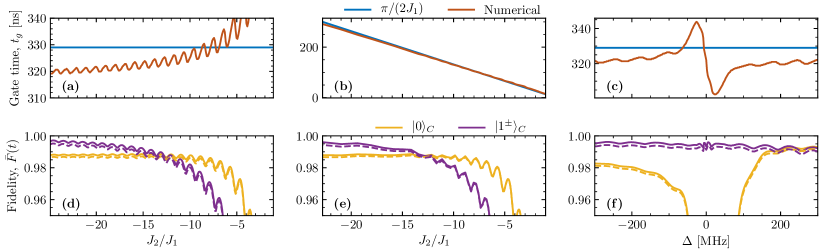
Figure 1: [(a)-(c)] Gate time as a function of the model parameters $J_{2}$, $1/J_{1}$, and $\Delta$. The blue lines indicates the analytical result of Eq. 7 and the red lines indicates the point of maximum average fidelity. [(d)-(e)] Average fidelities at the numerical gate time as a function of the model parameters $J_{2}$, $1/J_{1}$, and $\Delta$, both with (dashed lines) and without (solid lines) decoherence noise. The yellow lines indicates the fidelity when the gate is in the open configuration, while the purple line indicates that it is in the closed configuration.

In order to quantify the effectiveness of the gate, we use numerical simulations with realistic gate parameters for state-of-the-art superconducting circuits. In Fig. 4, we show simulations of the gate in a circuit with specific superconducting circuit parameters. We include decoherence noise occurring in superconducting circuits by considering the Lindblad master equation

$$\dot{\rho}=-i[H,\rho]+\gamma\sum_{j}\left[A_{l}\rho A_{l}^{\dagger}-\frac{1}{2}\{\rho,A_{l}^{\dagger}A_{l}\}\right],$$ (5)

where $\rho$ is the density matrix, $H$ is the Hamiltonian in Eq. 3, the curly brackets indicates the anticommutator, and the sum is taken over the eight collapse operators $A_{l}$: $\sigma_{j}^{z}$ inducing dephasing, and $\sigma_{j}^{-}$ inducing photon loss, with $j$ running over all qubits. We take the decoherence rate, $\gamma$, to be identical on all qubits with a state-of-the-art rate of $\gamma=$0.01\text{\,}\mathrm{MHz}$$, giving the qubits a lifetime of $100\text{\,}\mathrm{\SIUnitSymbolMicro s}$ Wang et al. (2019).

In order to measure the quality of the gate, we consider the average fidelity Nielsen (2002)

$$\bar{F}(t)=\frac{1}{5}+\frac{1}{80}\sum_{j=1}^{16}\text{Tr}\left(U_{\text{target}}U_{j}^{\dagger}U_{\text{target}}^{\dagger}\mathcal{E}_{t}(U_{j})\right),$$ (6)

which evaluates how well a quantum map, $\mathcal{E}_{t}$, approximates the target gate, $U_{\text{target}}$, over a uniform distribution of input quantum states, $U_{j}$. The target operator is either $U_{\text{open}}$ or $U_{\text{closed}}$ depending of the state of the control qubits, which is encoded in the initial density matrix $\rho(0)$. By solving the Lindblad master equation, Eq. 5 we obtain the density matrix at a later time, $\rho(t)$. This is done using the Python toolbox QuTiP Johansson et al. (2013). Having obtained the full density matrix we can then trace out the control degrees of freedom, yielding the desired quantum map $\mathcal{E}_{t}(\rho(0))=\text{Tr}_{T}(\rho(t))$. We chose the basis, $U_{j}$, of the average fidelity as all two-qubit Pauli operators on the form $(\sigma_{1}^{x})^{k}(\sigma_{1}^{z})^{l}(\sigma_{N}^{x})^{m}(\sigma_{N}^{z})^{n}$ for all combinations of $k,l,m,n\in\{0,1\}$.

Thus given a set of model parameters, the average fidelity can be calculated as a function of time for both set of gate configurations. In the case of the open gate, i.e., configuration $|0\rangle_{C}$, the average fidelity rises from some initial value to a maximum (unity for the perfect gate) at the gate time, which we denote $t_{g}$. Analytically, we expect this to be (see Supplementary Material sup for a derivation of this)

$$t_{g}=\frac{\pi}{|2J_{1}|};$$ (7)

however, for the simulations we find the best gate time numerically. In the case of the closed gate, i.e., the configuration $|1\rangle_{C}$, the average fidelity is initially unity and deviates only from this value due to leakage to the control qubits or as a result of decoherence noise.

In order to investigate the sensitivity of the parameter space, we vary the parameters $J_{1}$, $J_{2}$, and $\Delta$ and show the gate time and average fidelities at the gate time in Fig. 1. The simulation is done both with and without noise. In Figs. 1(a) and (d), we vary the coupling of the control qubits, $J_{2}\equiv J^{x}_{2}=J^{z}_{2}$, in the configuration $|1^{+}\rangle_{C}$, while keeping the remaining coupling constants at $J_{1}=$30\text{\,}\mathrm{MHz}$$. Setting $J_{2}^{x}=J_{2}^{z}$ is merely done for the simplicity of the numerical investigation and is not a requirement, as we will exploit later. From this simulation we observe that the numerical gate time is about 5% faster than the analytical, and for large $J_{2}/J_{1}$ we observe almost unity average fidelity for the closed configuration of the gate, and between 0.98 and 0.99 for the open configuration. In Figs. 1(b) and (e), we vary the coupling between the target qubits and the control qubits, i.e. $J_{1}$, while keeping the coupling between the control qubits constant at $J_{2}=$750\text{\,}\mathrm{MHz}$$, in the configuration $|1^{+}\rangle_{C}$. Again, we observe a slightly shorter numerical gate time, and fidelities of close to unity and just between 0.98 and 0.99 for the closed and open configuration respectively. In Figs. 1(c) and (f), we vary $J_{2}^{x}$ and keeping $J_{2}^{z}=$600\text{\,}\mathrm{MHz}$$ in the case of the gate being in the configuration $|1^{-}\rangle_{C}$ in order to effectively vary $\Delta$ around zero. We observe that the gate completely fails around zero, as it should, but we also conclude that we achieve a larger average fidelity (just above 0.99) for a positive detuning, i.e., $J_{2}^{z}>J_{2}^{x}$, rather than a negative detuning. However, for the case of $|1^{+}\rangle_{C}$, we find that the average fidelity is slightly larger when $J_{2}^{z}<J_{2}^{x}$. From the simulations, we also find that a different sign on the couplings $J_{1}$ and $J_{2}$ yields a slightly larger average fidelity.

The above mentioned simulations beg the question of why the average gate fidelities do not approach unity, even when the requirements mentioned in Sec. II.1 are fulfilled. The answer to this question is found together with the answer as to why the numerical gate time is shorter than the analytical gate time in Eq. 7. It all comes down to the fact that even though the state $|1\rangle|0\rangle_{C}|1\rangle$ is indeed an eigenstate of the Hamiltonian, it is also degenerate with the states $|1\rangle|1^{\mp}\rangle_{C}|0\rangle$ and $|0\rangle|1^{\mp}\rangle_{C}|1\rangle$ depending on the choice of $\Delta_{\pm}$ (note that these states are not the same as the configurations of the closed gate). This means that the system will oscillate between these three states, in a manner similar to how the open gate oscillates between states with a single excitation. However, the time scale for the oscillation of the double excitation is less than for the single excitation, with an oscillation time of about 90% of the analytical gate time. This means that some time between $0.9t_{g}$ and $t_{g}$ we will observe maximum average fidelity, less unity, depending on the configuration of the system.

This does, however, not mean that it is impossible to achieve perfect transfer for some states, in a well configured system. Namely as long as not both the input and output qubit are in a superposition state, the state is transfered perfectly, when disregarding decoherence noise.

Note that the resonance of the eigenstates mentioned above is the same resonance that makes the gate work to begin with, in that case it is the states $|1\rangle|0\rangle_{C}|0\rangle$, $|0\rangle|0\rangle_{C}|1\rangle$, and $|0\rangle|1^{\mp}\rangle_{C}|0\rangle$ that are in resonance.

III Possible physical realization

We wish to implement the Hamiltonian in Eq. 3, and thus the swapping gate, using superconducting circuits. As in the previous section, we will focus on implementing the case of $N=4$, but the idea is easily expanded to larger $N$.

III.1 Superconducting circuit

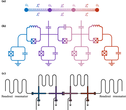
Figure 2: (a) The desired spin model as seen in Eq. 3. (b) The lumped circuit model for the super conducting circuit used to implement the above system. The crossed boxes represent Josephson junctions, the parallel lines are capacitors, and the curled wires are inductors. (c) Possible circuit design, consisting of four X-mon-style superconducting islands, all grounded and with control lines from below. The small green patches indicate Josephson junctions, while the bent wires represent inductors. The first and last qubits are connected to a readout resonator as well. The colors indicates which parts of the three models correspond to each other.

The circuit used to implement the system can be seen in Fig. 2(b). The circuit consists of four Transmon-type qubits Koch et al. (2007), which are all grounded and connected in series through Josephson junctions, with as small of a parasitic capacitance as possible. In parallel with the connecting Josephson junctions is either a capacitor or an inductor, alternating between these two. Additional qubits are added to the chain by connecting them through a Josephson junction and either a capacitor or an inductor. It is important that two connecting capacitances are not next to each other, since this will induce cross talk between the nodes. When there is only a capacitor between every other pair of nodes the capacitance matrix becomes block diagonal, which means that its inverse will be block diagonal as well. However, had there been capacitors between all nodes the capacitance matrix would have been tridiagonal, and its inverse would not necessarily be tridiagonal, which possibly yields cross talk, i.e., couplings other than nearest neighbor coupling. In reality, there will always be a parasitic capacitance between two nodes connected through a Josephson junction; however, not including these are equivalent to assuming $C_{i}\gg C_{i,i+1}$, where $C_{i}$ is the shunting capacitance of the $i$th qubit and $C_{i,i+1}$ is the parasitic capacitance between the $i$th and $(i+1)$th node. See Appendix A for a discussion on the emergence of cross talk due to capacitive couplings.

Instead of transmon qubits one could, in principle, have used other types of superconducting qubits such as the C-shunted qubit (or floxmons) Orlando et al. (1999); Mooij et al. (1999); van der Wal et al. (2000); You et al. (2007); Yan et al. (2016) or fluxonium Manucharyan et al. (2009).

For each node in the circuit, we have a related flux degree of freedom, which we denote $\phi_{i}$ Vool and Devoret (2017). Interactions between the qubits are induced by capacitors and inductors, which induce $XX$ couplings, and Josephson junctions which induce both $XX$ and $ZZ$ couplings. A detailed calculation going from the circuit design to the Hamiltonian in Eq. 3 can be found in the Supplementary Material sup . Since Josephson junctions are nonlinear inductors and thus induce both $XX$ and $ZZ$ couplings between the qubits, it might seem redundant to include inductors or capacitors in parallel with these. However, these are included such that it is possible to tune the $XX$ coupling without affecting the $ZZ$ coupling significantly.

In order to operate the gate successively, i.e., opening and closing the gate in an uninterrupted sequence, we need a scheme for preparing the state of the gate. We would like to be able to address the control qubits exclusively, i.e., opening and closing the gate independently of the target qubits. This is possible when the target qubits are detuned from the control qubits, i.e., $\Delta$ is sufficiently large, compared to the couplings between the control qubits and the target qubits. A large detuning can, in experiments, be obtained by tuning the external fluxes.

We can achieve control of the gate by driving the middle nodes. The driving is performed by adding an external field to the nodes through capacitors. The control lines are depicted in Fig. 2(c) as the wires left of the ground. This introduces an extra driving term to the Hamiltonian, which in the interaction picture takes the form

$$H_{d}(t)=\frac{A}{2}I(t)\left[(\sigma_{2}^{y}+\sigma_{3}^{y})\cos\delta t-(\sigma_{2}^{x}+\sigma_{3}^{x})\sin\delta t\right],$$ (8)

for an in-phase driving, where we have defined $\delta=\omega-\Omega_{1}$, $\omega$ is the driving frequency, and $I(t)$ is the envelope of the driving pulse. Like the rest of the Hamiltonian this term preserves the total spin of the two gate qubits, and hence it does not mix the singlet and triplet states. We can therefore ignore the singlet state $\left|1^{-}\right\rangle_{C}$, when starting from any of the triplet states shown in Fig. 3.

Figure 3: Sketch of the state of the control qubits. The states of the target qubits have not been added since $J_{1}\ll J_{2}$, and the fact that we wish to operate the gate on a timescale where the target qubits are stationary i.e. irrelevant for the difference in energy of the gate’s energy levels. One can further detune the gate from the target qubits by using the flux lines depicted in Fig. 2, thus effectively eliminating the coupling between the gate and the target qubits.

Rabi oscillations between the closed and open states are then generated by the driving, provided the driving frequency matches the energy difference $\omega=|\Omega-2J_{2}^{z}+2J_{2}^{x}|$ and $A\ll J_{2}^{z}$. A $\pi$ pulse would then shift between the $\left|0\right\rangle_{C}$ and $\left|1^{+}\right\rangle_{C}$ states in a few microseconds depending on the size of $A$. The energy difference between the open or closed states and the last state $\left|11\right\rangle_{C}$ are far enough from $\omega$ such that we do not populate this state by accident. Thus, using this scheme, we can drive between an open and closed gate using merely an external microwave drive. For a detailed calculation of the driving force see the Supplementary Material sup .

If we were to drive the system for an intermediate time between zero and one $\pi$ pulse, we would obtain a superposition of the open and closed gate. Suppose that we drive the Rabi oscillation for half a $\pi$ pulse, $t=\pi/2A$: In this case we would get the superposition

$$|1^{+}\rangle_{C}\rightarrow\frac{1}{\sqrt{2}}\left(|1^{+}\rangle_{C}+i|0\rangle_{C}\right).$$ (9)

In this case the gate would permit a superposition of the system being transferred and not. In the same way that the transferred state accumulates a phase during the transfer, so does the superposition gate. The phase obtained by the superposition gate is simply the energy difference between the open and closed state. Thus, we must include a phase factor of

$$e^{-i(\Omega_{2}-2J_{2}^{z}+2J_{2}^{x})t}$$ (10)

on the gate when evaluating the state.

A lumped circuit diagram is not enough for a possible realistic implementation and we therefore propose an experimental realistic chip design, which can be seen in Fig. 2(c). The chip consists of four X-mon-like superconducting islands Barends et al. (2013), each connected to the ground through a Transmon qubit, and each connected to a control line. All qubits are connected to its neighbor through a Josephson junction, and the two middle are close to one another in order to create a capacitive coupling, while the outer islands are farther from the middle islands in order to minimize the capacitive coupling, while being connected through an inductor each. The outer islands corresponds to the target qubits and are therefore connected to an LC resonator each, in order to be able to perform measurements on them. The two middle islands corresponds to the control qubits.

III.2 Leakage and infidelities

Because that we require a large coupling coefficient between the two control qubits, $J_{2}$, the superconducting circuit is vulnerable to leakage to higher excited states than the two lowest states. In order to investigate the amount of leakage in our system we simulate it with the control qubits being qutrits, i.e., including the three lowest states of the system. The simulation is done for realistic parameters which can be found in Table S1 of the Supplementary Material sup . The average fidelity is shown in Fig. 4, together with the results for the system with purely qubits.

From Fig. 4, we observe that the average fidelity is not affected significantly in the large picture; however, if we zoom in on the peak of the average fidelity in the open state, we observe that the average fidelity has indeed decreased in both cases of the open gate and the case of the $|1^{+}\rangle$-closed gate, while the fidelity of the $|1^{-}\rangle$-closed case has increased. In general, whether the inclusion of the second excited state in the gate will increase or decrease the fidelity is dependent on the parameters of the gate. However, as long as the anharmonicity remains large ($\mathcal{A}^{r}\gtrsim 0.1\%$ Koch et al. (2007)) the effect will be minimal, not changing the overall picture.

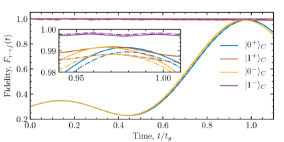
Figure 4: Average fidelity of the system with realistic parameters as a function of time. The simulations are done both for control qubits (solid lines) and qutrits (dashed dotted lines). The average fidelity is plotted for all possible configurations of the control qubits and qutrits. The $|0^{\pm}\rangle_{C}$ indicates the choice of detuning $\Delta_{\pm}$ and thus which of the open gates in Eq. 4 the simulation is done for. The inset shows a zoom of the peak of the average fidelity in the open configuration $|0\rangle_{C}$, i.e., around $t\sim t_{g}$.

Besides leakage to higher excited states capacitive couplings beyond nearest neighbor qubits possess the biggest threat to gate fidelity. We therefore consider the effect of cross talk on the average gate fidelities as seen in Fig. 5. From the simulation, we see that next-to-nearest couplings have no effect on the gate when it is in its closed configurations $|1^{\pm}\rangle_{C}$, and have only little effect when it is in its open configuration $|0\rangle_{C}$. In fact, the average fidelity increases a tiny amount until the next-to-nearest neighbor coupling is $\sim 3\%$ of the nearest neighbor coupling between the target qubits and the control qubits. This is consistent with the result of Ref. Loft et al. (2018). Next-to-next-to-nearest couplings, on the other hand, have a much more significant influence on the system when the coupling strength is above 2% of the target-control coupling, and we conclude that the gate fidelity decreases as the square of the next-to-next-to-nearest coupling strength. This is expected since the next-to-next-to-nearest coupling is a direct coupling of the input and output qubits.

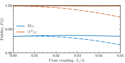
Figure 5: Average fidelities of the control qubits in both states for increasing strength of coupling beyond nearest neighbor coupling, $J_{c}$. The solid lines is with next-to-nearest couplings included, and the dash-dotted lines are with up to next-to-next-to-nearest neighbor coupling.

IV Extensions and outlook

Besides being used for the above mentioned swapping gate, the superconducting circuit is interesting in many other settings because it implements the most fundamental of all spin model structures: the linear spin chain. The linear chain is the obvious choice for a “quantum wire” in an implementation of quantum information processing, especially if configured for perfect state transfer over a fixed period of time Christandl et al. (2004). The superconducting circuit in Fig. 2 is a possible candidate for this application because of its straight forward scaling.

Consider the case where we want a model without any $ZZ$ couplings. One way to achieve this is simply to fine-tune the system and thus suppress the $ZZ$ couplings. However, there is an easier way: All the contributions to the $ZZ$ coupling stem from the Josephson junctions, and thus removing those will create a purely $XX$-coupled spin chain. One could even remove the capacitors and just couple the qubits through a series of inductors similar to the chain in Ref. Neill et al. (2018) or the one-dimensional tight-binding lattice for photons mentioned in Ref. Ningyuan et al. (2015), but with superconducting qubits instead of LC resonators in order to create a spin model and not a boson model. This circuit could also be used to investigate the Su-Schrieffer-Heeger (SSH) model Su et al. (1979); Heeger et al. (1988) defined on the dimerized one-dimensional lattice with two sites per unit cell, both in the strong and weak coupling limit in relation the the Zak phase as considered by Ref. Goren et al. (2018). It should be mentioned that we were not able to reproduce the lattice in Ref. Goren et al. (2018) using their suggested circuit because of the previously mentioned fact that the inverse of the capacitance matrix, with couplings entirely with capacitors, is not tridiagonal, which induces non-negligible cross talk, especially in the strong coupling limit. The occurrence of this problem is illuminated in Appendix A. Our circuit does not introduce this cross talk, and is therefore more suitable for the investigation of the SSH model.

The superconducting circuit presented here can also easily be molded into a box model where each qubit corresponds to a corner of the box and each edge a coupling. This is done simply by connecting the first and last superconducting island of the circuit, i.e., the blue and red islands in Fig. 2, with a Josephson junction and/or a capacitor depending on which kind of coupling one wishes to implement. In a realistic implementation, it might be necessary to place the X-mon superconducting island in a square pattern instead of a linear pattern, as seen in Fig. 2(c). Such a system could be used to engineering quantum spin liquids and many-body Majorana states Yang et al. (2018).

Lastly, we mention that even though we have tried to avoid cross talk up until now, it is possible to modify the circuit into having all-to-all $XX$ couplings by connecting all superconducting islands with capacitors. The most effective implementation of this would be in the box shape, since this avoids the use of 3D integration Rosenberg et al. (2017); Lu et al. (2019). For all-to-all $ZZ$ couplings, one would have to use 3D integration as all superconducting islands must be connected directly via Josephson junctions.

V Conclusion

We have investigated a linear chain of qubits and found that under the right configuration these can operate as a two-qubit swapping gate with different phases depending on the initial conditions. In particular we have focused on the case of four qubits and shown that it can create a swapping gate with a fidelity around 0.99, even when including realistic decoherence noise and leakage to higher excited states.

Furthermore, we have proposed a superconducting circuit which realizes the four-qubit spin chain. Both a lumped circuit model and a possible chip design using X-mon-style qubits have been presented and we have discussed how to operate this circuit between the different configurations of a given gate. Finally, we have discussed how the superconducting circuit can be modified in a simple manner to realize other models with Hamiltonians that have attracted considerable interest in recent times. This shows that the basic model and layout we propose may have extended utility in both quantum processing and quantum simulation research directions.

Appendix A Full capacitive couplings

In this appendix, we consider different cases of capacitive couplings between qubits. We consider both cases which yield couplings beyond nearest neighbor couplings and cases which yields only nearest neighbor couplings, as is desired in our case.

Consider the circuit in Fig. 6, which is $N$ qubits in series coupled with capacitors. This circuit yields a Lagrangian of

$$L= \sum_{n=1}^{N}\left(\frac{1}{2}C_{i}\dot{\phi}_{i}^{2}+E_{i}\cos\phi_{i}\right),$$ (11)

which yields a Hamiltonian of

$$H= 4\bm{p}^{T}K^{-1}\bm{p}-\sum_{n=1}^{N}E_{i}\cos\phi_{i}.$$ (12)

Now consider that we want identical couplings between all of the qubits: We therefore set $C_{i}=C^{\prime}_{i}=C$, which yields the following inverse capacitance matrix here for the simple case of $N=4$:

$$K^{-1}=\frac{1}{C}\begin{pmatrix}1&0&-1&1\\ 0&0&1&-1\\ -1&1&0&0\\ 1&-1&0&1\end{pmatrix}.$$ (13)

From this, we see that the desired nearest neighbor coupling simply disappears between some of the qubits, while couplings beyond nearest neighbor are significant. Increasing the number of qubits does not fix this. In fact, in all cases where $N+1$ is dividable with 3, the matrix is even singular. One could try to fix this simply by increasing size of the shunting capacitor $C^{\prime}_{i}$ of the qubit compared to the coupling capacitor $C_{i}$. Thus, for $C_{i}^{\prime}=10C_{i}=10C$, we get

$$K^{-1}\simeq\frac{1}{C}\begin{pmatrix}1&-0.1&0.01&-0.001\\ -0.1&1&-0.1&0.01\\ 0.01&-0.1&1&-0.1\\ -0.001&0.01&-0.1&1\end{pmatrix},$$ (14)

which does indeed seem to fix the problem. Consider now the case where we want to make a SSH chain, such as in Ref. Goren et al. (2018). In this case, we alternate the coupling between the qubits such that in the case of $N=6$

$$K=\begin{pmatrix}C^{\prime}_{1}&C&0&0&0&0\\ C&C^{\prime}_{2}&2C&0&0&0\\ 0&2C&C^{\prime}_{3}&C&0&0\\ 0&0&C&C^{\prime}_{4}&2C&0\\ 0&0&0&2C&C^{\prime}_{5}&C\\ 0&0&0&0&C&C^{\prime}_{6}\\ \end{pmatrix}.$$ (15)

For $C^{\prime}_{i}=C$, we obtain a result similar to Eq. 13 in the first example where some of the nearest neighbor couplings disappear, and couplings beyond this become large. This can be fixed using the approach mentioned above with $C\ll C_{i}^{\prime}$. The proposal of Ref. Goren et al. (2018) suggests to take $C\gg C_{i}^{{}^{\prime}}$ in order to enter the strong-coupling regime and realize a linear SSH chain. Given the above analysis, we cannot see how this is feasible without some other modifications to the circuit.

Figure 6: The circuit consists of $N$ qubits connected through capacitors of size $C_{i}$. Each transmon consists of a capacitor of size $C^{\prime}_{i}$ and a Josephson junction (usually a SQUID) of size $E_{i}$. The nodes of the circuit are denoted $n_{i}$.

In order to avoid couplings beyond nearest neighbor couplings, the superconducting qubits should instead be connected with inductors or connected with alternating inductors and capacitors in order to avoid cross talk. However, if one desires a SSH model, it is still not enough to alternate between the sizes of the inductors or capacitors if the chain is of finite length, due to end-point irregularities.

If the circuit is constructed with only capacitors on every other coupling between the qubits the capacitance matrix becomes block diagonal. Consider a block-diagonal matrix consisting of invertible matrices $\mathbf{K}_{i}$

$$K=\begin{pmatrix}\mathbf{K}_{1}&0&0&\cdots&0\\ 0&\mathbf{K}_{2}&0&\cdots&0\\ 0&0&\mathbf{K}_{3}&\cdots&0\\ \vdots&\vdots&\vdots&\ddots&0\\ 0&0&0&0&\mathbf{K}_{N}\\ \end{pmatrix},$$ (16)

which yields an inverse capacitance matrix of

$$K^{-1}=\begin{pmatrix}\mathbf{K}_{1}^{-1}&0&0&\cdots&0\\ 0&\mathbf{K}_{2}^{-1}&0&\cdots&0\\ 0&0&\mathbf{K}_{3}^{-1}&\cdots&0\\ \vdots&\vdots&\vdots&\ddots&0\\ 0&0&0&0&\mathbf{K}_{N}^{-1}\\ \end{pmatrix},$$ (17)

which is block diagonal as well. If the matrices $\mathbf{K}_{i}$ are $2\times 2$ the capacitance matrix yields only nearest neighbor couplings. The lack of couplings between the blocks of the matrix can be fixed by adding inductors between the blocks of qubits.

In the specific case of $N=4$ qubits discussed in the main text the capacitance matrix is given as

$$K=\begin{pmatrix}C_{1}&0&0&0\\ 0&C_{2}+C_{2,3}&-C_{2,3}&0\\ 0&-C_{2,3}&C_{2}+C_{2,3}&0\\ 0&0&0&C_{1}\end{pmatrix},$$ (18)

which yields an inverse capacitance matrix of

$$K^{-1}=\begin{pmatrix}1/C_{1}&0&0&0\\ 0&(C_{2}+C_{23})/C_{0}&-C_{2,3}/C_{0}&0\\ 0&-C_{2,3}/C_{0}&(C_{2}+C_{2,3})/C_{0}&0\\ 0&0&0&1/C_{1}\end{pmatrix},$$ (19)

where $C_{0}=C_{2}^{2}+2C_{2,3}C_{2}$. This yields only couplings between the middle two qubits.

References

- DiVincenzo (1995) D. P. DiVincenzo, Phys. Rev. A 51, 1015 (1995).
- Buluta et al. (2011) I. Buluta, S. Ashhab, and F. Nori, Reports on Progress in Physics 74, 104401 (2011).
- Gustavsson et al. (2013) S. Gustavsson, O. Zwier, J. Bylander, F. Yan, F. Yoshihara, Y. Nakamura, T. P. Orlando, and W. D. Oliver, Phys. Rev. Lett. 110, 040502 (2013).
- Reagor et al. (2018) M. Reagor, C. B. Osborn, N. Tezak, A. Staley, G. Prawiroatmodjo, M. Scheer, N. Alidoust, E. A. Sete, N. Didier, M. P. da Silva, E. Acala, J. Angeles, A. Bestwick, M. Block, B. Bloom, A. Bradley, C. Bui, S. Caldwell, L. Capelluto, R. Chilcott, J. Cordova, G. Crossman, M. Curtis, S. Deshpande, T. El Bouayadi, D. Girshovich, S. Hong, A. Hudson, P. Karalekas, K. Kuang, M. Lenihan, R. Manenti, T. Manning, J. Marshall, Y. Mohan, W. O’Brien, J. Otterbach, A. Papageorge, J.-P. Paquette, M. Pelstring, A. Polloreno, V. Rawat, C. A. Ryan, R. Renzas, N. Rubin, D. Russel, M. Rust, D. Scarabelli, M. Selvanayagam, R. Sinclair, R. Smith, M. Suska, T.-W. To, M. Vahidpour, N. Vodrahalli, T. Whyland, K. Yadav, W. Zeng, and C. T. Rigetti, Science Advances 4 (2018), 10.1126/sciadv.aao3603.
- Rol et al. (2017) M. A. Rol, C. C. Bultink, T. E. O’Brien, S. R. de Jong, L. S. Theis, X. Fu, F. Luthi, R. F. L. Vermeulen, J. C. de Sterke, A. Bruno, D. Deurloo, R. N. Schouten, F. K. Wilhelm, and L. DiCarlo, Phys. Rev. Applied 7, 041001 (2017).
- Sheldon et al. (2016a) S. Sheldon, E. Magesan, J. M. Chow, and J. M. Gambetta, Phys. Rev. A 93, 060302 (2016a).
- Chen et al. (2016) Z. Chen, J. Kelly, C. Quintana, R. Barends, B. Campbell, Y. Chen, B. Chiaro, A. Dunsworth, A. G. Fowler, E. Lucero, E. Jeffrey, A. Megrant, J. Mutus, M. Neeley, C. Neill, P. J. J. O’Malley, P. Roushan, D. Sank, A. Vainsencher, J. Wenner, T. C. White, A. N. Korotkov, and J. M. Martinis, Phys. Rev. Lett. 116, 020501 (2016).
- Barends et al. (2014) R. Barends, J. Kelly, A. Megrant, A. Veitia, D. Sank, E. Jeffrey, T. C. White, J. Mutus, A. G. Fowler, B. Campbell, Z. Chen, Y.and Chen, B. Chiaro, A. Dunsworth, C. Neill, P. OMalley, P. Roushan, A. Vainsencher, J. Wenner, A. N. Korotkov, A. N. Cleland, and J. M. Martinis, Nature 508, 500 (2014).
- Raussendorf and Harrington (2007) R. Raussendorf and J. Harrington, Phys. Rev. Lett. 98, 190504 (2007).
- Córcoles et al. (2015) A. D. Córcoles, E. Magesan, S. J. Srinivasan, A. W. Cross, M. Steffen, J. M. Gambetta, and J. M. Chow, Nature Communications 6, 6979 (2015).
- O’Brien et al. (2017) T. E. O’Brien, B. Tarasinski, and L. DiCarlo, npj Quantum Information 3, 39 (2017).
- Fowler et al. (2012) A. G. Fowler, M. Mariantoni, J. M. Martinis, and A. N. Cleland, Phys. Rev. A 86, 032324 (2012).
- Chow et al. (2011) J. M. Chow, A. D. Córcoles, J. M. Gambetta, C. Rigetti, B. R. Johnson, J. A. Smolin, J. R. Rozen, G. A. Keefe, M. B. Rothwell, M. B. Ketchen, and M. Steffen, Phys. Rev. Lett. 107, 080502 (2011).
- Li et al. (2008) J. Li, K. Chalapat, and G. S. Paraoanu, Phys. Rev. B 78, 064503 (2008).
- Rigetti and Devoret (2010) C. Rigetti and M. Devoret, Phys. Rev. B 81, 134507 (2010).
- Paraoanu (2006) G. S. Paraoanu, Phys. Rev. B 74, 140504 (2006).
- Kelly et al. (2014) J. Kelly, R. Barends, B. Campbell, Y. Chen, Z. Chen, B. Chiaro, A. Dunsworth, A. G. Fowler, I.-C. Hoi, E. Jeffrey, A. Megrant, J. Mutus, C. Neill, P. J. J. O’Malley, C. Quintana, P. Roushan, D. Sank, A. Vainsencher, J. Wenner, T. C. White, A. N. Cleland, and J. M. Martinis, Phys. Rev. Lett. 112, 240504 (2014).
- Chen et al. (2014) Y. Chen, C. Neill, P. Roushan, N. Leung, M. Fang, R. Barends, J. Kelly, B. Campbell, Z. Chen, B. Chiaro, A. Dunsworth, E. Jeffrey, A. Megrant, J. Y. Mutus, P. J. J. O’Malley, C. M. Quintana, D. Sank, A. Vainsencher, J. Wenner, T. C. White, M. R. Geller, A. N. Cleland, and J. M. Martinis, Phys. Rev. Lett. 113, 220502 (2014).
- Sheldon et al. (2016b) S. Sheldon, L. S. Bishop, E. Magesan, S. Filipp, J. M. Chow, and J. M. Gambetta, Phys. Rev. A 93, 012301 (2016b).
- McKay et al. (2016) D. C. McKay, S. Filipp, A. Mezzacapo, E. Magesan, J. M. Chow, and J. M. Gambetta, Phys. Rev. Applied 6, 064007 (2016).
- Dewes et al. (2012) A. Dewes, F. R. Ong, V. Schmitt, R. Lauro, N. Boulant, P. Bertet, D. Vion, and D. Esteve, Phys. Rev. Lett. 108, 057002 (2012).
- Salathé et al. (2015) Y. Salathé, M. Mondal, M. Oppliger, J. Heinsoo, P. Kurpiers, A. Potočnik, A. Mezzacapo, U. Las Heras, L. Lamata, E. Solano, S. Filipp, and A. Wallraff, Phys. Rev. X 5, 021027 (2015).
- Poletto et al. (2012) S. Poletto, J. M. Gambetta, S. T. Merkel, J. A. Smolin, J. M. Chow, A. D. Córcoles, G. A. Keefe, M. B. Rothwell, J. R. Rozen, D. W. Abraham, C. Rigetti, and M. Steffen, Phys. Rev. Lett. 109, 240505 (2012).
- Paik et al. (2016) H. Paik, A. Mezzacapo, M. Sandberg, D. T. McClure, B. Abdo, A. D. Córcoles, O. Dial, D. F. Bogorin, B. L. T. Plourde, M. Steffen, A. W. Cross, J. M. Gambetta, and J. M. Chow, Phys. Rev. Lett. 117, 250502 (2016).
- Vojta (2003) M. Vojta, Reports on Progress in Physics 66, 2069 (2003).
- Hu (1984) C.-K. Hu, Phys. Rev. B 29, 5103 (1984).
- Morita et al. (2018) K. Morita, T. Sugimoto, S. Sota, and T. Tohyama, Phys. Rev. B 97, 014412 (2018).
- Depenbrock et al. (2012) S. Depenbrock, I. P. McCulloch, and U. Schollwöck, Phys. Rev. Lett. 109, 067201 (2012).
- Marchukov et al. (2016) O. V. Marchukov, A. G. Volosniev, M. Valiente, D. Petrosyan, and N. T. Zinner, Nature Communications 7, 13070 (2016).
- (30) See Supplemental Material for a deriviation of the requirements for the gate both in the case of and , an in depth analysis of the circuit, a discussion of the state preparation driving scheme, a detailed calculation of the system with the second excited state included, and a table with realistic circuit parameters the corresponding spin parameters. The Supplementary Material includes Refs. Marchukov et al. (2016); Nield1994; Devoret1997; Vool and Devoret (2017); Warren1984; Steffen2003; Gambetta2011; Motzoi2013; Rebentrost2009; Khaneja2005; Motzoi2009.
- Möttönen et al. (2004) M. Möttönen, J. J. Vartiainen, V. Bergholm, and M. M. Salomaa, Phys. Rev. Lett. 93, 130502 (2004).
- Möttönen et al. (2005) M. Möttönen, J. J. Vartiainen, V. Bergholm, and M. M. Salomaa, “Transformation of quantum states using uniformly controlled rotations,” (2005), arXiv:quant-ph/0407010 .
- Babbush et al. (2018) R. Babbush, C. Gidney, D. W. Berry, N. Wiebe, J. McClean, A. Paler, A. Fowler, and H. Neven, Phys. Rev. X 8, 041015 (2018).
- Zanardi et al. (2000) P. Zanardi, C. Zalka, and L. Faoro, Phys. Rev. A 62, 030301 (2000).
- Wang et al. (2019) Z. Wang, S. Shankar, Z. Minev, P. Campagne-Ibarcq, A. Narla, and M. Devoret, Phys. Rev. Applied 11, 014031 (2019).
- Nielsen (2002) M. A. Nielsen, Physics Letters A 303, 249 (2002).
- Johansson et al. (2013) J. R. Johansson, P. D. Nation, and F. Nori, Comp. Phys. Comm. 184, 1234 (2013).
- Koch et al. (2007) J. Koch, T. M. Yu, J. Gambetta, A. A. Houck, D. I. Schuster, J. Majer, A. Blais, M. H. Devoret, S. M. Girvin, and R. J. Schoelkopf, Phys. Rev. A 76, 042319 (2007).
- Orlando et al. (1999) T. P. Orlando, J. E. Mooij, L. Tian, C. H. van der Wal, L. S. Levitov, S. Lloyd, and J. J. Mazo, Phys. Rev. B 60, 15398 (1999).
- Mooij et al. (1999) J. E. Mooij, T. P. Orlando, L. Levitov, L. Tian, C. H. van der Wal, and S. Lloyd, Science 285, 1036 (1999).
- van der Wal et al. (2000) C. H. van der Wal, A. C. J. ter Haar, F. K. Wilhelm, R. N. Schouten, C. J. P. M. Harmans, T. P. Orlando, S. Lloyd, and J. E. Mooij, Science 290, 773 (2000).
- You et al. (2007) J. Q. You, X. Hu, S. Ashhab, and F. Nori, Phys. Rev. B 75, 140515 (2007).
- Yan et al. (2016) F. Yan, S. Gustavsson, A. Kamal, J. Birenbaum, A. P. Sears, D. Hover, T. J. Gudmundsen, D. Rosenberg, G. Samach, S. Weber, J. L. Yoder, T. P. Orlando, J. Clarke, A. J. Kerman, and W. D. Oliver, Nature Communications 7, 12964 (2016).
- Manucharyan et al. (2009) V. E. Manucharyan, J. Koch, L. I. Glazman, and M. H. Devoret, Science 326, 113 (2009).
- Vool and Devoret (2017) U. Vool and M. H. Devoret, International Journal of Circuit Theory and Applications 45, 897 (2017).
- Barends et al. (2013) R. Barends, J. Kelly, A. Megrant, D. Sank, E. Jeffrey, Y. Chen, Y. Yin, B. Chiaro, J. Mutus, C. Neill, P. O’Malley, P. Roushan, J. Wenner, T. C. White, A. N. Cleland, and J. M. Martinis, Phys. Rev. Lett. 111, 080502 (2013).
- Loft et al. (2018) N. J. S. Loft, M. Kjaergaard, L. B. Kristensen, C. K. Andersen, T. W. Larsen, S. Gustavsson, W. D. Oliver, and N. T. Zinner, “High-fidelity conditional two-qubit swapping gate using tunable ancillas,” (2018), arXiv:1809.09049 .
- Christandl et al. (2004) M. Christandl, N. Datta, A. Ekert, and A. J. Landahl, Phys. Rev. Lett. 92, 187902 (2004).
- Neill et al. (2018) C. Neill, P. Roushan, K. Kechedzhi, S. Boixo, S. V. Isakov, V. Smelyanskiy, A. Megrant, B. Chiaro, A. Dunsworth, K. Arya, R. Barends, B. Burkett, Y. Chen, Z. Chen, A. Fowler, B. Foxen, M. Giustina, R. Graff, E. Jeffrey, T. Huang, J. Kelly, P. Klimov, E. Lucero, J. Mutus, M. Neeley, C. Quintana, D. Sank, A. Vainsencher, J. Wenner, T. C. White, H. Neven, and J. M. Martinis, Science 360, 195 (2018).
- Ningyuan et al. (2015) J. Ningyuan, C. Owens, A. Sommer, D. Schuster, and J. Simon, Phys. Rev. X 5, 021031 (2015).
- Su et al. (1979) W. P. Su, J. R. Schrieffer, and A. J. Heeger, Phys. Rev. Lett. 42, 1698 (1979).
- Heeger et al. (1988) A. J. Heeger, S. Kivelson, J. R. Schrieffer, and W. P. Su, Rev. Mod. Phys. 60, 781 (1988).
- Goren et al. (2018) T. Goren, K. Plekhanov, F. Appas, and K. Le Hur, Phys. Rev. B 97, 041106 (2018).
- Yang et al. (2018) F. Yang, L. Henriet, A. Soret, and K. Le Hur, Phys. Rev. B 98, 035431 (2018).
- Rosenberg et al. (2017) D. Rosenberg, D. Kim, R. Das, D. Yost, S. Gustavsson, D. Hover, P. Krantz, A. Melville, L. Racz, G. O. Samach, S. J. Weber, F. Yan, J. L. Yoder, A. J. Kerman, and W. D. Oliver, npj Quantum Information 3 (2017), https://doi.org/10.1038/s41534-017-0044-0.
- Lu et al. (2019) Y. Lu, N. Jia, L. Su, C. Owens, G. Juzeliūnas, D. I. Schuster, and J. Simon, Phys. Rev. B 99, 020302 (2019).