Characterizing the analogy between hyperbolic embedding and community structure of complex networks

Abstract

We show that the community structure of a network can be used as a coarse version of its embedding in a hidden space with hyperbolic geometry. The finding emerges from a systematic analysis of several real-world and synthetic networks. We take advantage of the analogy for reinterpreting results originally obtained through network hyperbolic embedding in terms of community structure only. First, we show that the robustness of a multiplex network can be controlled by tuning the correlation between the community structures across different layers. Second, we deploy an efficient greedy protocol for network navigability that makes use of routing tables based on community structure.

A wealth of recent publications provides evidence of the advantages that may arise from thinking of real-world networks as instances of random network models embedded in hidden metric spaces Serrano et al. (2008); Boguna et al. (2009). In this class of models, every node is represented by coordinates that identify its position in the underlying space, and the distance between pairs of nodes determines their likelihood of being connected. The most popular formulation of spatially embedded network models relies on hyperbolic geometry Krioukov et al. (2009, 2010). Hyperbolic network geometry emerges spontaneously from models of growing simplicial complexes Bianconi and Rahmede (2017). Hyperbolic geometry appears the natural choice for networks with broad degree distributions, under the hypothesis that the generating mechanism for edges in the network is a compromise between popularity of individual nodes and similarity among pairs of nodes Papadopoulos et al. (2012). Popularity is represented by the radial coordinate of nodes in the hyperbolic space, while similarity is accounted for by the difference between angular coordinates of pairs of nodes. Hyperbolic maps are useful in practical contexts, as generating efficient routing protocols in information networks Boguná et al. (2010), characterizing hierarchical organization of biochemical pathways in cellular networks Serrano et al. (2012a), and monitoring the evolution of the international trade network García-Pérez et al. (2016). However, thinking of networks as embedded in the hyperbolic space is important from the theoretical point of view too. Growing network models that rely on hyperbolic geometry provide a genuine explanation for the emergence of power-law degree distributions from local optimization principles only Papadopoulos et al. (2012). Further, recent work show that the main features of the percolation transition in multiplex networks can be predicted by simply accounting for inter-layer correlation among hyperbolic coordinates of nodes Kleineberg et al. (2016, 2017).

Popularity and similarity are core features of models used in network hyperbolic embedding. They are, however, central in another heavily used model in network science: the degree-corrected stochastic block model (SBM) Karrer and Newman (2011). The SBM assumes a hidden cluster structure where nodes are divided into a certain number of groups. This classification accounts for similarity, as pairs of nodes have different likelihoods of being connected depending on their group memberships. The degree correction provides instead a natural way of accounting for the popularity of the individual nodes. The SBM is generally considered in the context of graph clustering, representing a generative network model with built-in mesoscopic structure Fortunato (2010). The SBM is used in the formulation of principled community detection methods Peixoto (2017). These methods, in turn, are equivalent to other well-established techniques for community detection, giving therefore to the SBM a central role in the graph clustering business Newman (2016).

At least superficially, the analogy between the ideas of hyperbolic embedding and community structure is apparent. In a recent paper, Wang et al. showed that information about community structure can be used to improve accuracy and efficiency of standard algorithms for hyperbolic embedding Wang et al. (2016). Also, previous work was devoted to the development of network models embedded in hyperbolic geometry with the addition of a pre-imposed community structure Zuev et al. (2015); García-Pérez et al. (2018); Muscoloni and Cannistraci (2017). We are not aware, however, of previous attempts to investigate the theoretical and practical similarity of the two approaches when applied independently to the same network topology. This is the purpose of the present paper.

We assume that the topology of an undirected and unweighted network $G$ with $N$ nodes is fully specified by its adjacency matrix $A$, whose element $A_{i,j}=A_{j,i}=1$ if a connection between nodes $i$ and $j$ is present, or $A_{i,j}=A_{j,i}=0$, otherwise. The hyperbolic embedding of the network $G$ consists in a pair of coordinates $(r_{i},\theta_{i})$ for every node $i\in G$. The quantity $r_{i}$ is the radial coordinate of node $i$; $\theta_{i}$ is its angular coordinate. We assume that this information is at our disposal. The way we acquire such a knowledge depends on whether the network analyzed is synthetic or real. For synthetic graphs, we consider single instances of the popularity-similarity optimization model (PSOM) Papadopoulos et al. (2012), so that hyperbolic coordinates correspond to ground-truth values of the model. We analyze also several real networks, where coordinates of nodes are obtained by fitting graphs against the PSOM. In this second scenario, we either rely on embeddings publicly available Kleineberg et al. (2016); Papadopoulos et al. (2015a) or we apply publicly available algorithms to the graphs  Papadopoulos et al. (2015a). Details are provided in the Supplemental Material (SM). We remark that the PSOM is the model of reference in most of the hyperbolic embedding techniques. It assumes the existence of an underlying hyperbolic space, and consists in a random growing network model where nodes are connected depending on their distance, and the value of other model parameters, such as average degree $\langle k\rangle$, exponent $\gamma$ of the power-law degree distribution $P(k)\sim k^{-\gamma}$, and temperature $T$. When a real network is fitted against the PSOM, the parameters $\langle k\rangle$ and $\gamma$ of the model are determined on the basis of the observed network, while $T$ is treated as a free parameter Papadopoulos et al. (2015a). Its value may be set to the one that yields the best match between theoretical and numerical results for the distance dependent connection probability Papadopoulos et al. (2015b); when hyperbolic embedding is used in greedy routing, one may look for the $T$ value that results in the highest success rate Papadopoulos et al. (2015a). The radial coordinate $r_{i}$ of every node $i$ is uniquely identified by its degree $k_{i}$, hence $r_{i}$ doesn’t require to be truly learned. The angular coordinate $\theta_{i}$ for every node $i\in G$ is instead treated as a fitting parameter. There are various techniques to perform the fit, including approximated optimization algorithms Papadopoulos et al. (2015b, a), and ad-hoc heuristic methods Alanis-Lobato et al. (2016); Muscoloni et al. (2017).

In our analysis, we further assume to know the community structure of the graph $G$, consisting in a flat partition of the network into $C$ total communities, where every node $i\in G$ is associated with a discrete-valued coordinate $\sigma_{i}=1,\ldots,C$. Algorithms for community detection are numerous Fortunato (2010). Here, we rely on results obtained by three popular methods: the Louvain algorithm Blondel et al. (2008), Infomap Rosvall and Bergstrom (2008), and the algorithm by Ronhovde and Nussinov Ronhovde and Nussinov (2010). We remark that, in the degree-corrected SBM, the probability for nodes $i$ and $j$ to be connected is a function of $\sigma_{i}$, $\sigma_{j}$, $k_{i}$ and $k_{j}$. Hence, the graph $G$ can be thought as embedded into a community structure, where every node $i$ is de facto represented by the coordinates $(k_{i},\sigma_{i})$.

A direct comparison between the hyperbolic embedding and the community structure of the graph $G$ consists in a comparison between the coordinates of the individual nodes in the two representations. Further, as the degree of the nodes trivially matches in both representations, the comparison reduces only in matching angular coordinates $\theta$s and group memberships $\sigma$s. From the numerous empirical tests we conducted on both real and synthetic networks, two main conclusions emerge. First, networks usually considered in hyperbolic embedding applications are highly modular, in the sense that partitions found by community detection algorithms correspond to very large values of the modularity function $Q$ Newman and Girvan (2004) (see Figure 1 and  SM. Second, nodes within the same communities are likely to have similar angular coordinates. We note that this second finding is in line with what already shown in Ref. Wang et al. (2016). To quantify coherence among angular coordinates of nodes within the same community $g$, we first define the variables $\xi_{g}$ and $\phi_{g}$ with

$$\xi_{g}\;e^{\textrm{i}\,\phi_{g}}=\frac{1}{n_{g}}\,\sum_{j=1}^{N}\delta_{\sigma_{j},g}\,e^{\textrm{i}\,\theta_{j}}\;.$$ (1)

$\delta_{x,y}=1$ if $x=y$ and $\delta_{x,y}=0$, otherwise. The r.h.s. of Eq. (1) stands for the sums of vectors in the complex plane of the type $e^{\textrm{i}\,\theta}=\cos(\theta)+\textrm{i}\sin(\theta)$ of all nodes in group $g$. The vectorial sum is divided by the community size $n_{g}$ to obtain an average vector for the community. $\phi_{g}$ is the angular coordinate of community $g$. The module $0\leq\xi_{g}\leq 1$ indicates how coherent are the angular coordinates of the nodes within group $g$. Note that the definition of Eq. (1) resembles the one used for the order parameter of the Kuramoto model Kuramoto (1984). We finally measure the angular coherence of a partition as the weighted average

$$\bar{\xi}=\frac{1}{N}\,\sum_{g=1}^{C}n_{g}\xi_{g}\;.$$ (2)

By definition, we have that $0\leq\bar{\xi}\leq 1$. For all networks considered in our analysis (see Figure 1 and  SM), angular coherence is typically large.

Our empirical tests demonstrate that strong angular coherence within communities of strongly modular networks is a quite robust feature of both synthetic and real systems. This finding tells us that the analogy between community structure and hyperbolic embedding may extend beyond the mere similarity among their ingredients. The following examples show that the analogy is useful also in the interpretation of physical properties of networks and the design of practical algorithms on networks.

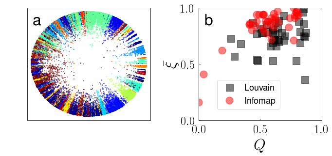
Figure 1: Hyperbolic embedding and community structure for real and synthetic networks. (a) We compare the hyperbolic embedding of the IPv4 Internet with its community structure. Every point represents a node in the largest connected component of the graph. Positions are determined by the radial and angular coordinates of the nodes in the hyperbolic embedding of the network Kleineberg et al. (2016). We use the best partition found by the Louvain algorithm to determine the community structure of the graph Blondel et al. (2008). The partition consists of $C=31$ communities. Colors of the points identify community memberships. The value of the modularity is $Q=0.61$, while angular coherence is $\bar{\xi}=0.72$. (b) We consider $39$ real-world networks and $2$ instances of the PSOM, and compare their community structure and hyperbolic embedding (see details in SM). The plot displays each network on the $(Q,\bar{\xi})$-plane. We show results obtained using Louvain (black squares) and Infomap (red circles) Rosvall and Bergstrom (2008).

Our first example regards the rephrasing, in terms of community structure only, of a result obtained by analyzing the hyperbolic embedding of multiplex networks. In two recent papers Kleineberg et al. (2016, 2017), Kleineberg and collaborators found that inter-layer correlation between hyperbolic coordinates of nodes in multiplex networks is a good predictor for the robustness of a system under targeted attack. Specifically, they found that, when correlation among angular coordinates is high, the percolation transition is smooth. Instead, multiplex networks characterized by a small value of inter-layer correlation exhibit abrupt percolation transitions. The finding was initially obtained for real-world multiplex networks. A theoretical explanation was then given in terms of a synthetic network model Kleineberg et al. (2017). To further support the analogy between hyperbolic embedding and community structure that we are arguing for in this paper, we replicated all results of Ref. Kleineberg et al. (2017) using community structure only. First, we analyzed the same real-world multiplex networks considered in Ref. Kleineberg et al. (2017). We found that their robustness can be predicted very well by the level of correlation among the community structures of the layers (see SM). Then, we provided a theoretical explanation. We replaced the network model by Kleineberg et al. with a variant of the SBM known in the literature as the Lancichinetti-Fortunato-Radicchi (LFR) benchmark graph Lancichinetti et al. (2008). The LFR model mostly differs from the standard SBM for relying on heterogeneous distributions of node degrees and community sizes. In our model for multiplex networks (see SM), we first generate a single LFR graph that is used as the topology for both layers. We then exchange the node labels in one layer to destroy edge overlap and degree-degree correlation. We consider two distinct scenarios. In the first case, we exchange the label of every node with the one of a randomly chosen node from the same community. This allows us to maintain perfect correlation between the community structure of the two layers. In the second case, we exchange the labels of a number of randomly sampled nodes such that the edge overlap between the layers equals the value obtained in the first randomization scheme. This second recipe completely destroys correlation between the community structures of the two layers. In Fig. 2a, we show the phase diagrams for instances of the multiplex model when relabeling uses information about the community structure of the graph. Here, the community structure is strong, in the sense that the fraction of external connections per node is only $\mu=0.1$. The transition appears smooth, and becomes smoother as the size of the model increases. This is an indication that, in the limit of infinitely large LFR graphs, the percolation transition is likely continuous. In Fig. 2b, we consider the second relabeling scheme that doesn’t account for community structure. The resulting diagrams indicate that the percolation transition is abrupt. The level of correlation among community structure of the two layers can be decreased by increasing $\mu$, so that community structure itself becomes less neat. This is done in Figs. 2c and d, where the transition appear abrupt no matter how the labels of the nodes are relabeled. In  SM, we report results for different parameter values of the LFR model. Results confirm our claim that the extent of correlation between the community structure of the layers of a multiplex can be used to explain robustness properties of the system under targeted attack.

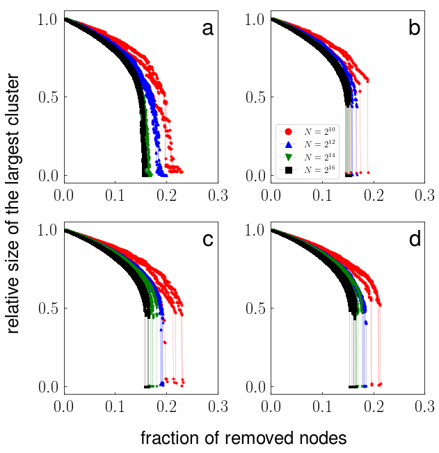
Figure 2: Robustness of multiplex networks with correlated community structure. We measure the relative size of the largest mutually connected cluster as a function of the fraction of nodes removed from the system. The synthetic multiplex graphs are obtained using the recipe described in the text, where two Lancichinetti-Fortunato-Radicchi (LFR) networks with size $N$ are coupled together. The LFR models are such that: the average degree is $\langle k\rangle=6$; the maximum degree is $k_{max}=\sqrt{N}$; node degrees $k$ obey a power-law distribution $P(k)\sim k^{-\gamma}$ with exponent $\gamma=2.6$; there are $C=\sqrt{N}$ communities of identical size $S=\sqrt{N}$. For every $N$, we show the results for five distinct instances of the model. (a) LFR graphs are generated with $\mu=0.1$. Labels are exchanged only among nodes within the same clusters. All nodes are considered for relabeling at least once. (b) Same as in panel a. However, relabeling of nodes is not constrained by community structure. The number of nodes that are relabeled is such that the edge overlap among layers is the same as in panel a (SM). (c and d) Same as in panels a and b, respectively, but for LFR graphs constructed using $\mu=0.3$.

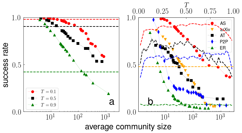
Figure 3: Performance of community-based routing. (a) We consider single instances of the growing network model of Ref. Papadopoulos et al. (2015b) with $N=5,000$ nodes, $\langle k\rangle=5$, and degree exponent $\gamma=2.1$. Different symbols and colors refer to different values of the temperature $T$. The plot shows how success rate of the community-based greedy routing strategy changes as a function the average size of the communities. Communities are identified using the algorithm by Ronhovde and Nussinov Ronhovde and Nussinov (2010). Their number can be varied by changing the resolution level of the algorithm. Dashed lines are obtained on the same networks but using hyperbolic greedy routing. (b) Same as in panel a, but for real networks. We consider the following networks: the Internet at the level of autonomous systems (AS) Leskovec et al. (2005); the worldwide air transportation network (AT) Guimerà et al. (2005); the European road network (ER) Šubelj and Bajec (2011); the peer-to-peer network (P2P) Ripeanu and Foster (2002); the arXiv collaboration network De Domenico et al. (2015a). For all the networks (except arXiv) the dashed lines are obtained by varying the temperature $T$ in the algorithm for hyperbolic embedding introduced in Ref. Papadopoulos et al. (2015a); for the arXiv network the dashed line shows the result for the optimum hyperbolic coordinates whose data was available in Kleineberg et al. (2016). Details can be found in SM.

Our second example focuses on greedy routing Boguna et al. (2009); Boguná et al. (2010). To be brief, the scenario considered is the following. A packet originated by node $s$ must be delivered to node $t$. The packet can navigate the network by walking at each step on an edge. The packet moves on the network till it reaches its destination $t$, or it visits twice the same node. In the first case, the packet is correctly delivered. In the second case, the packet is considered lost, and it is discarded. The goal of a good routing strategy is to deliver packets with high probability and with a small number of steps, for any randomly chosen pair of source and target nodes $s$ and $t$. Hyperbolic embedding turns out to be very useful in the formulation of a greedy strategy, where individual steps are determined on the basis of the distance among nodes in the hyperbolic space. Specifically, if a message is at node $i$, then the next move will be on the node

$$j^{\,(i)}_{(best)}=\arg\,\min_{j\in\mathcal{N}_{i}}d(j,t)\;,$$ (3)

where $\mathcal{N}_{i}$ is the set of neighbors of $i$, and $d(j,t)$ is the distance between nodes $j$ and $t$. The greedy technique is computationally feasible as every node needs to know only the identity and the geometric coordinates of its neighbors. The regimes of effectiveness of the routing method have been systematically studied in artificial network models Boguna et al. (2009). The technique has been proven to be extremely effective on some real-world topologies Boguna et al. (2009); Boguná et al. (2010). We devised a new greedy routing protocol that makes use of the cluster structure of a network instead of its hyperbolic embedding. Specifically, we replaced the definition of distance in the hyperbolic space between nodes with the fitness

$$d(j,t)=\beta D_{\sigma_{j},\sigma_{t}}-(1-\beta)\ln{k_{j}}\;,$$ (4)

where $k_{j}$ is the degree of node $j$, and $\sigma_{j}$ and $\sigma_{t}$ are the indices of the communities of nodes $j$ and $t$, respectively. $D_{\sigma_{j},\sigma_{t}}$ is the length of the shortest path between communities $\sigma_{j}$ and $\sigma_{t}$ calculated on a weighted supernetwork in which supernodes are communities of the original network. Each pair of supernodes $g$ and $q$ is connected with a superedge with weight $1-\ln{\rho_{g,q}}$; here $\rho_{g,q}$ is the probability that, in the original network, a randomly chosen node in community $g$ has an edge to community $q$ (see SM). The term $\ln{k_{j}}$ in Eq. (4) serves to perform degree correction. The factor $0\leq\beta\leq 1$ serves to control the relative importance of one factor over the other. $\beta$ plays a similar role as of the temperature $T$ in hyperbolic routing protocols Papadopoulos et al. (2015a), and its value may be appropriately chosen with the goal of optimizing the success rate in the delivery of messages (see SM). The routing protocol based on Eq. (4) is still computationally efficient as long as the total number of communities $C$ grows sub-linearly with the size of the graph $N$. In the extreme case, where every community is formed by a single node, so that $C=N$, the method will be $100\%$ accurate in delivering packets, but also computationally expensive. In Figure 3, we display the performance of community-based greedy routing as a function of the mean size of the communities. We study the performance on both synthetic and real-world networks. The number of communities is tuned by changing the resolution parameter in the algorithm by Ronhovde and Nussinov Ronhovde and Nussinov (2010). Success rates of the community-based greedy protocol are always very good, as long as communities are not too large.

In summary, we showed that looking at a network as embedded in a hyperbolic geometry is similar, both in theory and practice, to pretending that the network is organized into communities, provided that community structure is detected by a method that accounts for the degree of the nodes. Our finding provides evidence that the inter-community structure in networks may have geometric organization, meaning that at the global level, geometry dominates, while at the local scale, community memberships prevail. Thus, real networks may be modeled by a graphon Lovász (2012) consisting of a mixture of latent-spatial and block-like structures. This fundamental model has the potential to generate further understanding of physical processes, such as spreading and synchronization, in real networks.

I Supplemental Material

I.1 Hyperbolic embedding and community detection

In table S1, we provide a list of all networks considered in our analysis.

We obtain hyperbolic coordinates of networks in the following way. For real networks, we either rely on embeddings publicly available Kleineberg et al. (2016); Papadopoulos et al. (2015a) or we apply publicly available algorithms to the graphs  Papadopoulos et al. (2015a). Urls of electronic resources for all networks are provided in table S1. In the hyperbolic embeddings that we performed, we made use of the algorithm provided in https://bitbucket.org/dk-lab/2015_code_hypermap. As prescribed in Ref. Papadopoulos et al. (2015a), the value of the temperature $T$ used in the embedding corresponds to the one leading to maximal success rate in greedy routing  Boguna et al. (2009); Boguná et al. (2010) (see section below). We further consider two instances of the popularity-similarity optimization model (PSOM) Papadopoulos et al. (2012). They are generated using different values of the model parameters. The code to generate instances of the PSOM has been taken from https://www.cut.ac.cy/eecei/staff/f.papadopoulos.

We use three distinct methods for detecting communities in networks: the Louvain algorithm Blondel et al. (2008), Infomap Rosvall and Bergstrom (2008), and the algorithm by Ronhovde and Nussinov Ronhovde and Nussinov (2010). Louvain and Infomap are used in the analysis about the relation between hyperbolic embedding and community structure (see Table S1). The algorithm by Ronhovde and Nussinov is used in the analysis of greedy routing. For Louvain and Infomap we rely on the algorithms implemented in the library http://igraph.org/python. We consider always the “best” (i.e., the one with maximum modularity for Louvain , the one with minimum description length for Infomap) partitions found by the algorithms. The implementation of the algorithm by Ronhovde and Nussinov was taken from http://www.elemartelot.org/index.php/programming/cd-code. We chose this algorithm to study greedy routing as it allows for a finer tuning of the resolution of the community structure than the other two algorithms. After obtaining the modular structure from this algorithm, we perform an additional step to improve the quality of communities: If there is any community with size one we change the community label of the only member of that community to the label of its highest degree neighbor.

Table S1: Relation between community structure and hyperbolic embedding in real and synthetic networks. From left to right, we report: name of the network, size of the giant component $N$, number of communities $C$ identified by the Louvain algorithm, value of the modularity $Q$ corresponding to the Louvain partition, angular coherence $\bar{\xi}$ of the Louvain partition, number of communities $C$ identified by Infomap, value of the modularity $Q$ corresponding to the Infomap partition, angular coherence $\bar{\xi}$ of the Infomap partition, reference(s) of the papers where the dataset was reported and/or where hyperbolic coordinates of the network were obtained, urls of the websites where the corresponding data can be downloaded. If the url is denoted by ^∗, this means that data were obtained from a private communication and they are available upon request from the authors of Ref. Garzía-Pérez et al. (2018).

		Louvain			Infomap
network	$N$	$C$	$Q$	$\bar{\xi}$	$C$	$Q$	$\bar{\xi}$	Refs.	url
IPv4 Internet	$37,542$	$31$	$0.61$	$0.72$	$1,625$	$0.47$	$0.94$	Kleineberg et al. (2016)	http://koljakleineberg.wordpress.com/materials
IPv6 Internet	$5,143$	$19$	$0.48$	$0.53$	$418$	$0.41$	$0.86$	Kleineberg et al. (2016)	http://koljakleineberg.wordpress.com/materials
C. Elegans, layer 1	$248$	$9$	$0.65$	$0.70$	$29$	$0.61$	$0.83$	Kleineberg et al. (2016); Chen et al. (2006); De Domenico et al. (2015a)	http://koljakleineberg.wordpress.com/materials
C. Elegans, layer 2	$258$	$9$	$0.50$	$0.82$	$23$	$0.46$	$0.84$	Kleineberg et al. (2016); Chen et al. (2006); De Domenico et al. (2015a)	http://koljakleineberg.wordpress.com/materials
C. Elegans, layer 3	$278$	$7$	$0.44$	$0.87$	$11$	$0.42$	$0.86$	Kleineberg et al. (2016); Chen et al. (2006); De Domenico et al. (2015a)	http://koljakleineberg.wordpress.com/materials
D. Melanogaster, layer 1	$752$	$17$	$0.64$	$0.82$	$70$	$0.59$	$0.91$	Kleineberg et al. (2016); Stark et al. (2006); De Domenico et al. (2015b)	http://koljakleineberg.wordpress.com/materials
D. Melanogaster, layer 2	$633$	$17$	$0.64$	$0.72$	$68$	$0.60$	$0.89$	Kleineberg et al. (2016); Stark et al. (2006); De Domenico et al. (2015b)	http://koljakleineberg.wordpress.com/materials
arXiv, layer 1	$1,537$	$32$	$0.87$	$0.78$	$130$	$0.81$	$0.94$	Kleineberg et al. (2016); De Domenico et al. (2015c)	http://koljakleineberg.wordpress.com/materials
arXiv, layer 2	$2,121$	$35$	$0.86$	$0.74$	$190$	$0.79$	$0.96$	Kleineberg et al. (2016); De Domenico et al. (2015c)	http://koljakleineberg.wordpress.com/materials
arXiv, layer 3	$129$	$10$	$0.81$	$0.88$	$17$	$0.78$	$0.93$	Kleineberg et al. (2016); De Domenico et al. (2015c)	http://koljakleineberg.wordpress.com/materials
arXiv, layer 4	$3,669$	$46$	$0.82$	$0.69$	$290$	$0.74$	$0.91$	Kleineberg et al. (2016); De Domenico et al. (2015c)	http://koljakleineberg.wordpress.com/materials
arXiv, layer 5	$608$	$23$	$0.85$	$0.86$	$61$	$0.79$	$0.96$	Kleineberg et al. (2016); De Domenico et al. (2015c)	http://koljakleineberg.wordpress.com/materials
arXiv, layer 6	$336$	$17$	$0.84$	$0.96$	$38$	$0.80$	$0.98$	Kleineberg et al. (2016); De Domenico et al. (2015c)	http://koljakleineberg.wordpress.com/materials
Physician, layer 1	$106$	$8$	$0.51$	$0.78$	$13$	$0.52$	$0.80$	Kleineberg et al. (2017)	http://koljakleineberg.wordpress.com/materials
Physician, layer 2	$113$	$10$	$0.56$	$0.79$	$14$	$0.55$	$0.77$	Kleineberg et al. (2017)	http://koljakleineberg.wordpress.com/materials
Physician, layer 3	$110$	$9$	$0.60$	$0.53$	$18$	$0.59$	$0.72$	Kleineberg et al. (2017)	http://koljakleineberg.wordpress.com/materials
SacchPomb, layer 1	$751$	$21$	$0.79$	$0.53$	$86$	$0.73$	$0.83$	Kleineberg et al. (2016); Stark et al. (2006); De Domenico et al. (2015b)	http://koljakleineberg.wordpress.com/materials
SacchPomb, layer 2	$182$	$13$	$0.82$	$0.79$	$28$	$0.78$	$0.91$	Kleineberg et al. (2016); Stark et al. (2006); De Domenico et al. (2015b)	http://koljakleineberg.wordpress.com/materials
SacchPomb, layer 3	$2,340$	$25$	$0.52$	$0.78$	$119$	$0.47$	$0.88$	Kleineberg et al. (2016); Stark et al. (2006); De Domenico et al. (2015b)	http://koljakleineberg.wordpress.com/materials
SacchPomb, layer 4	$819$	$11$	$0.60$	$0.69$	$67$	$0.56$	$0.88$	Kleineberg et al. (2016); Stark et al. (2006); De Domenico et al. (2015b)	http://koljakleineberg.wordpress.com/materials
Human brain, layer 1	$85$	$5$	$0.62$	$0.87$	$8$	$0.62$	$0.92$	Kleineberg et al. (2017)	http://koljakleineberg.wordpress.com/materials
Human brain, layer 2	$78$	$6$	$0.55$	$0.85$	$8$	$0.56$	$0.88$	Kleineberg et al. (2017)	http://koljakleineberg.wordpress.com/materials
Rattus, layer 1	$1,866$	$32$	$0.69$	$0.71$	$129$	$0.65$	$0.87$	Kleineberg et al. (2016); Stark et al. (2006); De Domenico et al. (2015b)	http://koljakleineberg.wordpress.com/materials
Rattus, layer 2	$529$	$20$	$0.85$	$0.75$	$61$	$0.80$	$0.93$	Kleineberg et al. (2016); Stark et al. (2006); De Domenico et al. (2015b)	http://koljakleineberg.wordpress.com/materials
Air/Train, layer 1	$69$	$5$	$0.34$	$0.68$	$6$	$0.19$	$0.62$	Kleineberg et al. (2017)	http://koljakleineberg.wordpress.com/materials
Air/Train, layer 2	$67$	$6$	$0.26$	$0.73$	$5$	$0.04$	$0.41$	Kleineberg et al. (2017)	http://koljakleineberg.wordpress.com/materials
ARK200909	$24,091$	$29$	$0.62$	$0.77$	$980$	$0.53$	$0.94$	Papadopoulos et al. (2015a)	http://bitbucket.org/dk-lab/2015_code_hypermap
ARK201003	$26,307$	$29$	$0.62$	$0.71$	$1,070$	$0.52$	$0.94$	Papadopoulos et al. (2015a)	http://bitbucket.org/dk-lab/2015_code_hypermap
ARK201012	$29,333$	$28$	$0.60$	$0.80$	$1,171$	$0.49$	$0.94$	Papadopoulos et al. (2015a)	http://bitbucket.org/dk-lab/2015_code_hypermap
Enron emails	$33,696$	$291$	$0.58$	$0.66$	$1,546$	$0.52$	$0.82$	Leskovec et al. (2009); Garzía-Pérez et al. (2018)	∗
Music chords	$2,476$	$8$	$0.29$	$0.57$	$6$	$0.00$	$0.16$	Garzía-Pérez et al. (2018); Serrà et al. (2012)	∗
OpenFights Air Transp.	$3,397$	$26$	$0.65$	$0.89$	$167$	$0.61$	$0.95$	Garzía-Pérez et al. (2018); Kunegis (2013)	∗
Human Metabolites	$1,436$	$18$	$0.67$	$0.78$	$101$	$0.62$	$0.90$	Garzía-Pérez et al. (2018); Serrano et al. (2012b)	∗
Human HI-II-14 proteome	$4,100$	$42$	$0.47$	$0.54$	$334$	$0.43$	$0.80$	Garzía-Pérez et al. (2018); Rolland et al. (2014)	∗
AS Internet	$23,748$	$24$	$0.60$	$0.78$	$994$	$0.52$	$0.94$	Garzía-Pérez et al. (2018); Claffy et al. (2009)	∗
AS Oregon Interent, $T=0.58$	$6,474$	$31$	$0.63$	$0.66$	$412$	$0.54$	$0.88$	Leskovec et al. (2005)	http://snap.stanford.edu/data/as.html
Air Transportation, $T=0.14$	$3,618$	$36$	$0.69$	$0.93$	$246$	$0.64$	$0.97$	Guimerà et al. (2005)	http://seeslab.info/downloads
P2P, $T=0.92$	$6,299$	$19$	$0.47$	$0.77$	$598$	$0.41$	$0.85$	Ripeanu and Foster (2002)	http://snap.stanford.edu/data/p2p-Gnutella08.html
Euro Roads, $T=0.28$	$1,039$	$25$	$0.86$	$0.36$	$134$	$0.77$	$0.71$	Šubelj and Bajec (2011)	http://konect.uni-koblenz.de/networks/subelj_euroroad
PSOM, $\langle k\rangle=5$, $\gamma=2.1$, $T=0.1$	$4,114$	$40$	$0.85$	$0.99$	$248$	$0.77$	$1.00$	Papadopoulos et al. (2012)	http://www.cut.ac.cy/eecei/staff/f.papadopoulos
PSOM, $\langle k\rangle=5$, $\gamma=2.1$, $T=0.9$	$4,180$	$30$	$0.70$	$0.75$	$461$	$0.58$	$0.85$	Papadopoulos et al. (2012)	http://www.cut.ac.cy/eecei/staff/f.papadopoulos

I.2 Community structure and robustness of real-world multiplex networks

We performed the same type of analysis as in Ref. Kleineberg et al. (2017) by studying the relation between system robustness and “geometric” correlations among the network layers in real multiplex networks. We just replaced hyperbolic embedding with community structure. Specifically, given a multiplex network composed of two layers, we first detect communities in the largest connected component of both layers independently by using either Louvain or Infomap. Correlation between the community structure of the layers is measured using the normalized mutual information (NMI) defined in Ref. Danon et al. (2005). As the number of nodes in the layers may be different, in the computation of the NMI values, we considered only nodes appearing in both layers. We finally used the obtained NMI values in the scatter plots of Fig. S1. We find that the robustness of the various networks can be predicted equally well by looking at correlations among either hyperbolic coordinates or community memberships of the nodes in the two layers (see panels a–c). Further, we find that NMI values in the various representations are strongly correlated (panels d–e).

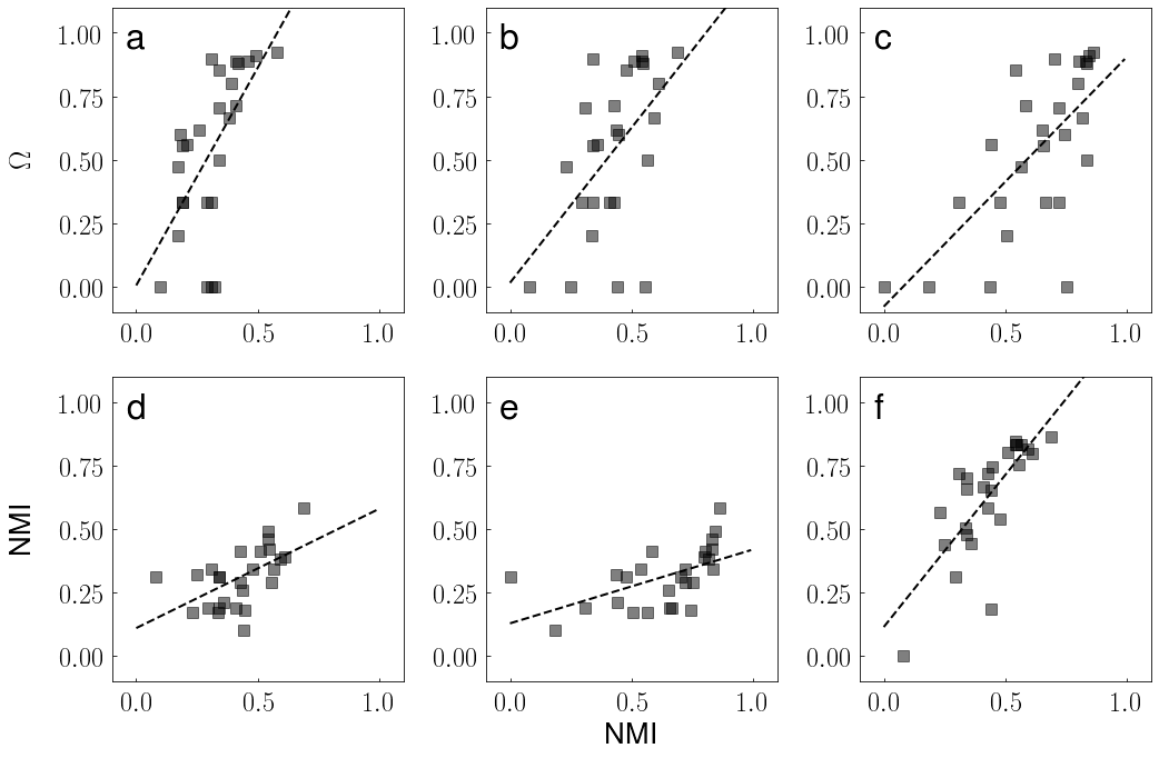
Figure S1: Community structure and robustness of real multiplex networks. We consider the $26$ multiplex networks analyzed in Ref. Kleineberg et al. (2017). As in Ref. Kleineberg et al. (2017), we rely on the quantity $\Omega$ as a proxy to evaluate the robustness of a given multiplex network. $\Omega=(\Delta N-\Delta N_{rs})/(\Delta N+\Delta N_{rs})$, where $\Delta N$ and $\Delta N_{rs}$ are respectively the widow sizes of the transitions in targeted and random percolation processes on the network. $\Omega$ values for the various networks have been taken from the supplemental material of Ref. Kleineberg et al. (2017). The normalized mutual information (NMI) serves to quantify similarity between the embedding of the nodes in the two layers. Values of the NMI for hyperbolic embedding have also been taken from the supplemental material of Ref. Kleineberg et al. (2017). We calculated instead NMI values among the community structures found for the layers of a multiplex using the definition provided in Ref. Danon et al. (2005). Communities in each layer are found using either Louvain or Infomap. (a) As a reference, we reproduced the same plot as in Fig. 4 of Ref. Kleineberg et al. (2017), where each network represents a point in the $($NMI, $\Omega)$-plane. The dashed line is obtained with simple linear regression. The correlation coefficient calculated from the data points is $r=0.63$. (b) Same as in panel a, but for NMI values calculated using the community structures found by the Louvain algorithm. Here $r=0.54$. (c) Same as in panel b, but for NMI values calculated using the community structures found by Infomap. We measured $r=0.68$ in this case. (d, e, and f) We compare NMI values obtained using the various embedding methods. The various panels represent: (d) Louvain vs. hyperbolic ($r=0.56$); (e) Infomap vs. hyperbolic ($r=0.55$); (f) Infomap vs. Louvain ($r=0.76$).

I.3 Multiplex networks with correlated community structure

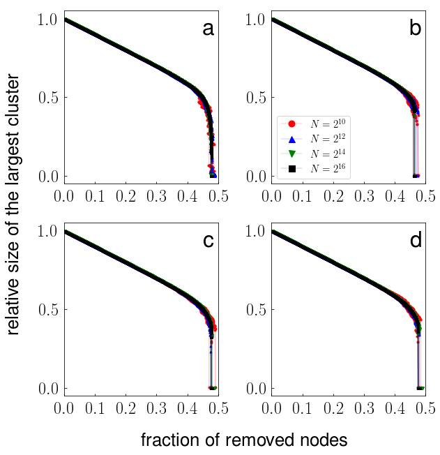
Figure S2: Robustness of multiplex networks with correlated community structure. We measure the relative size of the largest mutually connected cluster as a function of the fraction of nodes removed from the system. The synthetic multiplex graphs were obtained using the recipe described in the text, where two Lancichinetti-Fortunato-Radicchi (LFR) models with size $N$ are coupled together. The LFR models are such that: the average degree is $\langle k\rangle=6$ and the maximum degree is $k_{max}=6$, so that degree of all nodes is $k=6$; communities have identical size $S=64$. For every value of $N$ we show the results for five distinct instances of the model. (a) LFR graphs are generated with $\mu=0.1$. Labels are exchanged only among nodes within the same clusters. (b) Same as in panel a. However, relabeling of nodes is allowed among all nodes in the network. Probabilities of relabeling in panels a and b are such that the edge overlap among layers is the same for both models. (c and d) Same as in panels a and b, respectively, but for LFR graphs constructed using $\mu=0.3$.

The first step in the creation of a single instance of our multiplex model consists in generating a single instance of the Lancichinetti-Fortunato-Radicchi (LFR) model Lancichinetti et al. (2008). The LFR model is a variant of the degree-corrected stochastic block model. The model allows to generate single-layer networks with built-in community structure, where both the degree distribution $P(k)$ and community size distribution $P(S)$ are power-law functions, i.e., $P(k)\sim k^{-\gamma}$ and $P(S)\sim S^{-\beta}$. In addition to the exponents $\gamma$ and $\beta$, in the generation of one instance of the LFR model, one needs to specify the value of several parameters, including: average degree $\langle k\rangle$, maximum degree $k_{max}$, minimum $s_{min}$ and maximum $s_{max}$ community size, size of the network $N$, and the mixing parameter $\mu$. The mixing parameter $0\leq\mu\leq 1$ specifies the fraction of edges that a single node shares with nodes outside its own community. This parameter plays a fundamental role to determine how strong the community structure is. Low values of $\mu$ correspond to a strong community structure. As $\mu$ increases, community structure becomes fuzzy. The maximal value of $\mu$ for which planted community structure is exactly recoverable is bounded by a quantity calculated in Ref. Radicchi (2018). In our simulations, we use $\mu=0.1$ to represent a regime of strong community structure, and $\mu=0.3$ for regime of loose community structure. These values have been chosen arbitrarily, thinking to the application of the model here. For example, we didn’t use $\mu$ values too close to zero to avoid the presence of disconnected components.

Once a single instance of the LFR model is generated, we use that instance to define the topology of both layers of the multiplex. Node labels of the two layers are initially identical, so that the adjacency matrices of the two layers are identical. We then start relabeling nodes of one layer only. As already mentioned in the main text, we use two different strategies for relabeling. In the first strategy, we make use of the known community structure. In essence, in the relabeling procedure, the label of every node is exchanged with the one of another node randomly chosen from the same community. In the other procedure instead, the constraint on the group memberships is not used. This second variant corresponds to the same model already considered in Refs. Radicchi (2015); Osat et al. (2017). In this second variant, we perform a number of label swaps such that the value of the edge overlap among the two layers is comparable with the one obtained in the first variant of the model. Both variants of the multiplex model essentially lead to very small values of edge overlap and degree-degree correlation between layers. The first variant, however, preserves perfect correlation between the community structure of the two layers, while the second variant destroys it completely.

The robustness of single instances of the multiplex model described above are then studied as in Ref. Kleineberg et al. (2017). Every node $i$ in the network has associated the score $K_{i}=\max{(k_{i}^{(1)},k_{I}^{(2)})}$, with $k_{i}^{(x)}$ the degree of node $i$ in layer $x$. Nodes are then ranked in descending order according to this score, with ties randomly broken. The top node is removed from the network. After every removal, the score is $K_{i}$ of every node $i$ still in the system is recomputed. Further, the relative size of the mutually connected giant component is evaluated to construct a percolation phase diagram Buldyrev et al. (2010).

We considered various sets of parameters for the generation of the LFR model. All of them provide the same type of message. When the community structure is strong (i.e., small $\mu$ values), the model with correlated community structure undergoes a smooth percolation transition. If correlation in community structure is destroyed, the transition becomes abrupt. If the community structure is not strong (i.e., large $\mu$ values), then both relabeling schemes lead to an abrupt transition. The result is valid also for LFR models with homogenous degree distribution (see Figure S2).

I.4 Greedy routing

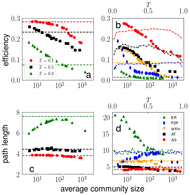
Figure S3: Same analysis as in Figure 3 of the main text. Performance is measured in terms of efficiency (panels a and b), and the average path length of successfully delivered packets (panels c and d).

As already considered in Refs. Boguna et al. (2009); Boguná et al. (2010), we immagine that a packet is traveling from the source node $s$ to the target node $t$ in a network with $N$ nodes and adjacency matrix $A$. The packet moves on edges of the network, performing a single hop at each stage of the dynamics. Greedy routing relies on a definition of “distance” between pairs of nodes in the network. At every stage $r$ of the dynamics towards the target node $t$, a packet sitting on node $p_{r}=i$ choose to move to the node $j^{\,(i)}_{(best)}$ defined in Eq. (4) of the main text. In essence, $j^{\,(i)}_{(best)}$ is the neighbor of node $i$ that has minimal distance to the target node $t$. In our numerical simulations, we avoid immediate backtracking walks of the packet, therefore node $j^{\,(i)}_{(best)}=p_{r+1}\neq p_{r-1}$, i.e., cannot be equal to the node visited before node $i$; this condition improves significantly (not shown) the performance of both methods considered in this paper. The packet continues to travel until one of these two conditions is met: (i) the packet arrives at destination after $R$ steps, i.e., $p_{R}=t$; (ii) the packet visits twice the same node, i.e., $p_{r}=p_{v}$, with $v<r$. Condition (i) corresponds to success. Condition (ii) represents failure and the packet is discarded. To evaluate performance of the routing protocol, we use at least $B=10,000$ numerical simulations. In each simulation, source $s$ and target $t$ nodes are randomly chosen among the nodes in the giant connected component of the network. We quantify three different metrics of performance:

• The success rate $z$ , i.e., the fraction of packets correctly delivered. This is a metric of performance introduced in Ref. Boguna et al. (2009). Results for this metric are presented in Figure 3 of the main text.

• The average value of $\langle R\rangle$, i.e., the average length of the paths for successfully delivered packets. This metric of performance was also introduced in Ref. Boguna et al. (2009). Results for this metric are presented in Figures S3c and d.

• Efficiency $\eta=z\,\langle 1/R\rangle$, where $\langle 1/R\rangle$ represents the mean value of the inverse of the path length obtained for each of the successfully delivered packets. This definition of $\eta$ is based on a metric of performance introduced in Ref. Muscoloni et al. (2017). Results for this metric are presented in Figures S3a and b.

It is worth noting that the efficiency measure (which is a balance between success rate and path length) shows similar results as those of the success rate (Figure S3a and b); this is because for almost all the networks of Figure S3, the path length does not change remarkably as the mean community size or the temperature is altered (Figures S3c and d). Thus, the success rate results (investigated in Figure 3 of the main text) are sufficient to assess the performance of the two routing methods investigated in this paper.

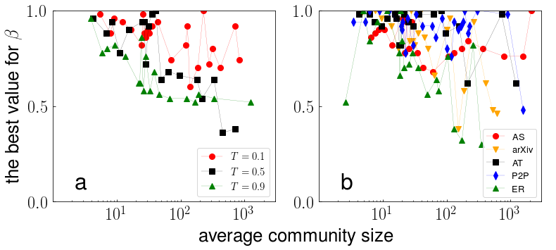
Figure S4: Same analysis as in Figure 3 of the main text. For each modular structure the $\beta$ value for which we obtained the highest success rate is reported.

In the standard application of network hyperbolic embedding, the distance between pairs of nodes is given by their distance in the hyperbolic space Boguna et al. (2009); Boguná et al. (2010). In our community-based routing protocol, we substituted the distance in the hyperbolic space with the analogous quantity based on the a priori given community structure of the graph. Specifically, we define the weight between the connected modules $g$ and $q$ as

$$w_{g,q}=1-\ln{\rho_{g,q}}\qquad\textrm{ , if }\rho_{g,q}>0\;,$$ (S1)

where

$$\rho_{g,q}=\frac{\sum_{i>j}A_{i,j}\delta_{\sigma_{i},g}\delta_{\sigma_{j},q}}{\sum_{i>j}A_{i,j}\delta_{\sigma_{i},g}}\;.$$ (S2)

In the above equation, $\delta_{x,y}=1$, if $x=y$, while $\delta_{x,y}=0$, otherwise; $A_{i,j}=A_{j,i}=1$ if nodes $i$ and $j$ are connected, while $A_{i,j}=A_{j,i}=0$, otherwise; $\sigma_{i}$ is the group membership of node $i$ according to the given community structure. Eq. (S2) is the ratio between the total number of edges shared between nodes within communities $g$ and $q$, and the total degree of nodes in community $g$. $\rho_{g,q}$ can be also interpreted as the probability that following a random edge of a random node in module $g$ we reach a node in module $q$. We consider each community as a supernode, and the network as a supernetwork composed of supernodes connected with weighted superedges. The weight of the superedge between supernodes $g$ and $q$ is defined in Eq. (S1). Then, we find the length of the shortest paths between every pair of supernodes. This operation relies on the algorithm by Johnson Johnson (1977). The output is a full matrix $D$ that includes the distances between every pair of modules. The generic element $D_{g,q}$ of this matrix contains a sum of weights defined in Eq. (S1), which is basically equivalent to a sort of expected path length between communities $g$ and $q$, under the hypothesis that connections were generated according to the stochastic block model Karrer and Newman (2011). Given that we are at node $i$ at stage $r$ of the trajectory of the packet, the “distance” between a neighbor $j$ of node $i$ and the target $t$ is finally defined as

$$d_{j,t}= \,\beta D_{\sigma_{j},\sigma_{t}}$$

$$+(1-\beta)\left\{\left[1-\log{\left(k_{j}\,\rho_{\sigma_{i},\sigma_{j}}\right)}\right]-\left[1-\log{\left(\rho_{\sigma_{i},\sigma_{j}}\right)}\right]\right\}$$ (S3)

$$= \,\beta D_{\sigma_{j},\sigma_{t}}-(1-\beta)\ln{k_{j}}$$ (S4)

where $k_{j}$ is the degree of node $j$, and $0\leq\beta\leq 1$. The previous expression defines a measure of “distance” between node $j$ and module $\sigma_{t}$. This is computed as a distance between modules $\sigma_{j}$ and $\sigma_{t}$, but corrected for the fact that we are aware of the degree of node $j$. This definition of distance is motivated by the degree-corrected stochastic block model in which the probability that following a randomly chosen edge from community $\sigma_{j}$ we reach a node in community $\sigma_{j^{\prime}}$ is proportional to $k_{j}\,\rho_{\sigma_{j},\sigma_{j^{\prime}}}$. Note that we are aware also of the degrees of nodes $i$ and $t$, but this information is not helpful in the protocol. The factor $\beta$ serves to weight the importance of the community structure vs. the degree of the individual nodes in the definition of distance. This factor can be tuned appropriately to optimize the success rate of the greedy routing protocol. Optimal values used in our simulations are displayed in Figure S4. As Figure S4 illustrates, the most optimum value of $\beta$ depends on the network structure and also on the considered modular structure; more specifically, $\beta$ is more likely to be close to 1 for networks with lower temperatures (or effectively those with higher clustering coefficients) and for modular structures with smaller mean community sizes.

References

- Serrano et al. (2008) M Angeles Serrano, Dmitri Krioukov, and Marián Boguná, “Self-similarity of complex networks and hidden metric spaces,” Physical Review Letters 100, 078701 (2008).
- Boguna et al. (2009) Marian Boguna, Dmitri Krioukov, and Kimberly C Claffy, “Navigability of complex networks,” Nature Physics 5, 74–80 (2009).
- Krioukov et al. (2009) Dmitri Krioukov, Fragkiskos Papadopoulos, Amin Vahdat, and Marián Boguná, “Curvature and temperature of complex networks,” Physical Review E 80, 035101 (2009).
- Krioukov et al. (2010) Dmitri Krioukov, Fragkiskos Papadopoulos, Maksim Kitsak, Amin Vahdat, and Marián Boguná, “Hyperbolic geometry of complex networks,” Physical Review E 82, 036106 (2010).
- Bianconi and Rahmede (2017) Ginestra Bianconi and Christoph Rahmede, “Emergent hyperbolic network geometry,” Scientific Reports 7 (2017).
- Papadopoulos et al. (2012) Fragkiskos Papadopoulos, Maksim Kitsak, M Ángeles Serrano, Marián Boguná, and Dmitri Krioukov, “Popularity versus similarity in growing networks,” Nature 489, 537–540 (2012).
- Boguná et al. (2010) Marián Boguná, Fragkiskos Papadopoulos, and Dmitri Krioukov, “Sustaining the internet with hyperbolic mapping,” Nature Communications 1, 62 (2010).
- Serrano et al. (2012a) M Ángeles Serrano, Marián Boguñá, and Francesc Sagués, “Uncovering the hidden geometry behind metabolic networks,” Molecular BioSystems 8, 843–850 (2012a).
- García-Pérez et al. (2016) Guillermo García-Pérez, Marián Boguñá, Antoine Allard, and M Ángeles Serrano, “The hidden hyperbolic geometry of international trade: World trade atlas 1870–2013,” Scientific reports 6, 33441 (2016).
- Kleineberg et al. (2016) Kaj-Kolja Kleineberg, Marián Boguná, M Ángeles Serrano, and Fragkiskos Papadopoulos, “Hidden geometric correlations in real multiplex networks,” Nature Physics 12, 1076–1081 (2016).
- Kleineberg et al. (2017) Kaj-Kolja Kleineberg, Lubos Buzna, Fragkiskos Papadopoulos, Marián Boguñá, and M Ángeles Serrano, “Geometric correlations mitigate the extreme vulnerability of multiplex networks against targeted attacks,” Physical Review Letters 118, 218301 (2017).
- Karrer and Newman (2011) Brian Karrer and Mark EJ Newman, “Stochastic blockmodels and community structure in networks,” Physical Review E 83, 016107 (2011).
- Fortunato (2010) Santo Fortunato, “Community detection in graphs,” Physics reports 486, 75–174 (2010).
- Peixoto (2017) Tiago P Peixoto, “Bayesian stochastic blockmodeling,” arXiv preprint arXiv:1705.10225 (2017).
- Newman (2016) MEJ Newman, “Equivalence between modularity optimization and maximum likelihood methods for community detection,” Physical Review E 94, 052315 (2016).
- Wang et al. (2016) Zuxi Wang, Qingguang Li, Fengdong Jin, Wei Xiong, and Yao Wu, “Hyperbolic mapping of complex networks based on community information,” Physica A: Statistical Mechanics and its Applications 455, 104–119 (2016).
- Zuev et al. (2015) Konstantin Zuev, Marián Boguñá, Ginestra Bianconi, and Dmitri Krioukov, “Emergence of soft communities from geometric preferential attachment,” Scientific reports 5, 9421 (2015).
- García-Pérez et al. (2018) Guillermo García-Pérez, M. Ángeles Serrano, and Marián Boguñá, “Soft communities in similarity space,” Journal of Statistical Physics (2018).
- Muscoloni and Cannistraci (2017) Alessandro Muscoloni and Carlo Vittorio Cannistraci, “A nonuniform popularity-similarity optimization (npso) model to efficiently generate realistic complex networks with communities,” arXiv preprint arXiv:1707.07325 (2017).
- Papadopoulos et al. (2015a) Fragkiskos Papadopoulos, Rodrigo Aldecoa, and Dmitri Krioukov, “Network geometry inference using common neighbors,” Physical Review E 92, 022807 (2015a).
- Papadopoulos et al. (2015b) Fragkiskos Papadopoulos, Constantinos Psomas, and Dmitri Krioukov, “Network mapping by replaying hyperbolic growth,” IEEE/ACM Transactions on Networking (TON) 23, 198–211 (2015b).
- Alanis-Lobato et al. (2016) Gregorio Alanis-Lobato, Pablo Mier, and Miguel A Andrade-Navarro, “Efficient embedding of complex networks to hyperbolic space via their laplacian,” Scientific reports 6, 30108 (2016).
- Muscoloni et al. (2017) Alessandro Muscoloni, Josephine Maria Thomas, Sara Ciucci, Ginestra Bianconi, and Carlo Vittorio Cannistraci, “Machine learning meets complex networks via coalescent embedding in the hyperbolic space,” Nature Communications 8, 1615 (2017).
- Blondel et al. (2008) Vincent D Blondel, Jean-Loup Guillaume, Renaud Lambiotte, and Etienne Lefebvre, “Fast unfolding of communities in large networks,” Journal of statistical mechanics: theory and experiment 2008, P10008 (2008).
- Rosvall and Bergstrom (2008) Martin Rosvall and Carl T Bergstrom, “Maps of random walks on complex networks reveal community structure,” Proceedings of the National Academy of Sciences 105, 1118–1123 (2008).
- Ronhovde and Nussinov (2010) Peter Ronhovde and Zohar Nussinov, “Local resolution-limit-free potts model for community detection,” Phys. Rev. E 81, 046114 (2010).
- Newman and Girvan (2004) Mark EJ Newman and Michelle Girvan, “Finding and evaluating community structure in networks,” Physical Review E 69, 026113 (2004).
- Kuramoto (1984) Yoshiki Kuramoto, Chemical oscillations, waves, and turbulence (Dover Publications, New York, 1984).
- Lancichinetti et al. (2008) Andrea Lancichinetti, Santo Fortunato, and Filippo Radicchi, “Benchmark graphs for testing community detection algorithms,” Physical review E 78, 046110 (2008).
- Leskovec et al. (2005) Jure Leskovec, Jon Kleinberg, and Christos Faloutsos, “Graphs over time: densification laws, shrinking diameters and possible explanations,” in Proceedings of the eleventh ACM SIGKDD international conference on Knowledge discovery in data mining (ACM, 2005) pp. 177–187.
- Guimerà et al. (2005) R. Guimerà, S. Mossa, A. Turtschi, and L. A. N. Amaral, “The worldwide air transportation network: Anomalous centrality, community structure, and cities’ global roles,” Proceedings of the National Academy of Sciences 102, 7794–7799 (2005).
- Šubelj and Bajec (2011) L. Šubelj and M. Bajec, “Robust network community detection using balanced propagation,” The European Physical Journal B 81, 353–362 (2011).
- Ripeanu and Foster (2002) Matei Ripeanu and Ian Foster, “Mapping the gnutella network: Macroscopic properties of large-scale peer-to-peer systems,” in Peer-to-Peer Systems, edited by Peter Druschel, Frans Kaashoek, and Antony Rowstron (Springer Berlin Heidelberg, Berlin, Heidelberg, 2002) pp. 85–93.
- De Domenico et al. (2015a) Manlio De Domenico, Mason A Porter, and Alex Arenas, “Muxviz: a tool for multilayer analysis and visualization of networks,” Journal of Complex Networks 3, 159–176 (2015a).
- Lovász (2012) László Lovász, Large networks and graph limits, Vol. 60 (American Mathematical Soc., 2012).
- Garzía-Pérez et al. (2018) Guillermo Garzía-Pérez, Marian Boguna, and Serrano M. Ángeles, “Multiscale unfolding of real networks by geometric renormalization,” Nature Physics -, – (2018).
- Chen et al. (2006) Beth L Chen, David H Hall, and Dmitri B Chklovskii, “Wiring optimization can relate neuronal structure and function,” Proceedings of the National Academy of Sciences of the United States of America 103, 4723–4728 (2006).
- Stark et al. (2006) Chris Stark, Bobby-Joe Breitkreutz, Teresa Reguly, Lorrie Boucher, Ashton Breitkreutz, and Mike Tyers, “Biogrid: a general repository for interaction datasets,” Nucleic acids research 34, D535–D539 (2006).
- De Domenico et al. (2015b) Manlio De Domenico, Vincenzo Nicosia, Alexandre Arenas, and Vito Latora, “Structural reducibility of multilayer networks,” Nature communications 6, 6864 (2015b).
- De Domenico et al. (2015c) Manlio De Domenico, Andrea Lancichinetti, Alex Arenas, and Martin Rosvall, “Identifying modular flows on multilayer networks reveals highly overlapping organization in interconnected systems,” Physical Review X 5, 011027 (2015c).
- Leskovec et al. (2009) Jure Leskovec, Kevin J Lang, Anirban Dasgupta, and Michael W Mahoney, “Community structure in large networks: Natural cluster sizes and the absence of large well-defined clusters,” Internet Mathematics 6, 29–123 (2009).
- Serrà et al. (2012) Joan Serrà, Álvaro Corral, Marián Boguñá, Martín Haro, and Josep Ll Arcos, “Measuring the evolution of contemporary western popular music,” Scientific reports 2, 521 (2012).
- Kunegis (2013) Jérôme Kunegis, “Konect: the koblenz network collection,” in Proceedings of the 22nd International Conference on World Wide Web (ACM, 2013) pp. 1343–1350.
- Serrano et al. (2012b) M Ángeles Serrano, Marián Boguná, and Francesc Sagués, “Uncovering the hidden geometry behind metabolic networks,” Molecular biosystems 8, 843–850 (2012b).
- Rolland et al. (2014) Thomas Rolland, Murat Taşan, Benoit Charloteaux, Samuel J Pevzner, Quan Zhong, Nidhi Sahni, Song Yi, Irma Lemmens, Celia Fontanillo, Roberto Mosca, et al., “A proteome-scale map of the human interactome network,” Cell 159, 1212–1226 (2014).
- Claffy et al. (2009) K. Claffy, Y. Hyun, K. Keys, M. Fomenkov, and D. Krioukov, “Internet mapping: From art to science,” in 2009 Cybersecurity Applications Technology Conference for Homeland Security (2009) pp. 205–211.
- Danon et al. (2005) Leon Danon, Albert Diaz-Guilera, Jordi Duch, and Alex Arenas, “Comparing community structure identification,” Journal of Statistical Mechanics: Theory and Experiment 2005, P09008 (2005).
- Radicchi (2018) Filippo Radicchi, “Decoding communities in networks,” Phys. Rev. E 97, 022316 (2018).
- Radicchi (2015) Filippo Radicchi, “Percolation in real interdependent networks,” Nature Physics 11, 597 (2015).
- Osat et al. (2017) Saeed Osat, Ali Faqeeh, and Filippo Radicchi, “Optimal percolation on multiplex networks,” Nature Communications 8, 1540 (2017).
- Buldyrev et al. (2010) Sergey V Buldyrev, Roni Parshani, Gerald Paul, H Eugene Stanley, and Shlomo Havlin, “Catastrophic cascade of failures in interdependent networks,” Nature 464, 1025 (2010).
- Johnson (1977) Donald B Johnson, “Efficient algorithms for shortest paths in sparse networks,” Journal of the ACM (JACM) 24, 1–13 (1977).