Strong disorder in nodal semimetals: Schwinger-Dyson–Ward approach

Björn Sbierski and Christian Fräßdorf Dahlem Center for Complex Quantum Systems and Institut für Theoretische Physik, Freie Universität Berlin, D-14195, Berlin, Germany
(March 19, 2024)
Abstract

The self-consistent Born approximation quantitatively fails to capture disorder effects in semimetals. We present an alternative, simple-to-use non-perturbative approach to calculate the disorder induced self-energy. It requires a sufficient broadening of the quasiparticle pole and the solution of a differential equation on the imaginary frequency axis. We demonstrate the performance of our method for various paradigmatic semimetal Hamiltonians and compare our results to exact numerical reference data. For intermediate and strong disorder, our approach yields quantitatively correct momentum resolved results. It is thus complementary to existing RG treatments of weak disorder in semimetals.

Introduction.—Semimetals with point-like Fermi surface are by now an established research field in condensed matter physics. Well-studied examples are two-dimensional (2d) Dirac fermions in graphene Novoselov et al. (2005), 3d Weyl fermions in spin-orbit coupled compounds Bernevig (2015), or parabolic band touching points in Bernal-stacked bilayer graphene McCann and Koshino (2013). Many experimental properties of semimetals rely on the presence of impurities or disorder, ubiquitous in solid state realizations, but under control in cold atom setups via speckle potentials Volchkov et al. (2018). For example, in undoped graphene the non-zero density-of-states is purely disorder generated Das Sarma et al. (2011). Likewise, in ARPES experiments it is the disorder, which broadens the spectral function at the nodal point and modifies its dispersion away from it. Another example is a disorder driven phase transition between a semimetallic and a metallic phase in 3d Weyl fermions Syzranov and Radzihovsky (2018). In the following, motivated by the observables described above, we focus on single-particle properties.

Theoretically, however, the currently available analytical methods for disordered semimetals yield unsatisfactory results. Weak disorder in semimetals can be treated using the perturbative Wilsonian momentum shell renormalization group (RG) as pioneered in the context of 2d Dirac systems by Ref. Ludwig et al. (1994). The starting point of this approach is the functional integral formalism that can be disorder averaged after the fermions have been replicated. The bosonic disorder field is then eliminated in favor of a four-fermion pseudo-interaction whose coupling constant flows as high energy shells are integrated out perturbatively. The drawback of the perturbative RG method is its inapplicability in the strong disorder regime and the difficulty to extract quantitative information about observables from the abstract RG flow. Another standard approach to disorder is the non-perturbative self-consistent Born approximation (SCBA). For metals, its validity relies on the smallness of the parameter $1/k_{F}l$ that quantifies the suppression of diagrams with crossed disorder lines omitted in SCBA Bruus and Flensberg (2004). Here, $k_{F}$ is the Fermi momentum and $l$ the mean free path. However, for semimetals with $k_{F}\!=\!0$, the SCBA cannot be justified Ostrovsky et al. (2006); Aleiner and Efetov (2006).

In this work, we propose a novel non-perturbative approach to disorder, systematically going beyond the SCBA but free of its above restrictions. Our approach is applicable for strong and intermediate Gaussian disorder where it yields a quantitatively accurate and momentum dependent self-energy. For semimetals, it is thus complementary to the RG approach. We start from the Fermi-Bose field theory mentioned above, but we do not integrate out the disorder field. Instead we derive an exact Schwinger-Dyson equation Peskin and Schröder (1995); Kopietz et al. (2010) for the fermionic self-energy, which is closed by replacing the Fermi-Bose three-vertex with the help of a Ward-identity. This replacement is justified for strong disorder only. We arrive at a set of ordinary differential equations on the imaginary frequency axis that can be easily solved numerically. We apply this Schwinger-Dyson–Ward (SDW) approach for various paradigmatic semimetals and compare our results to exact numerical reference data computed with a dedicated momentum space version of the kernel polynomial method. We also compare our results to the SCBA and a semi-classical approximation for strong disorder.

Model and main result.—We consider a generic two-band semimetal Hamiltonian $H_{0}(\vec{k})$ with a degeneracy point at $\vec{k}=0$ located at zero energy, $H_{0}(\vec{k}\!=\!0)\!=\!0$. For simplicity, we assume an isotropic dispersion $\pm E_{0}(k)$ with particle-hole symmetry. These assumptions are not crucial in the following but valid for many popular choices of $H_{0}(\vec{k})$ like Dirac nodes.

We add a smoothly correlated disorder potential $V(\vec{r})$ which is assumed to be diagonal in band space. Its correlation length $\xi$ represents the disorder puddle’s typical linear extent. We define the fundamental energy scale $E_{\xi}\!=\!E_{0}(k\!=\!1/\xi)$. For the statistical properties of $V$, we assert a Gaussian probability distribution $P\left[V\right]$ and define the disorder average of a quantity $Q[V]$ as $\left\langle Q\right\rangle_{dis}=\int\mathcal{D}VQ[V]P\!\left[V\right]$. We assume the disorder correlator $\mathcal{K}(\vec{r}-\vec{r}^{\prime})$ to have a Gaussian shape

$$\mathcal{K}(\vec{r}-\vec{r}^{\prime})=\left\langle V(\vec{r})V(\vec{r}^{\prime})\right\rangle_{dis}\!=\!\frac{W^{2}E_{\xi}^{2}}{(2\pi)^{d/2}}e^{-\frac{1}{2}|\vec{r}-\vec{r}^{\prime}|^{2}/\xi^{2}}.$$ (1)

The dimensionless parameter $W$ quantifies the strength of disorder. It relates the typical potential in a puddle $\sim\sqrt{\langle V(\vec{r})^{2}\rangle_{dis}}$ to the kinetic energy of a particle confined to the puddle’s volume. We refer to $W\ll 1$ as weak and $W\gg 1$ as strong disorder, respectively. We are interested in the zero-temperature retarded Green function $G_{V}^{R}(\omega)=(\omega+i\eta-H_{0}-V)^{-1}$ and, in particular, in its disorder average $\langle G_{V}^{R}\rangle_{dis}\equiv G^{R}$ ,

$\displaystyle G^{R}(\omega,\vec{k})$ $\displaystyle=\frac{1}{\omega+i\eta-H_{0}(\vec{k})-\Sigma^{R}(\vec{k},\omega)},$ (2)

at the nodal point energy $\omega=0$. This defines the disorder induced self-energy $\Sigma^{R}(\vec{k},\omega)$. Our main result is a self-consistency equation for the self-energy on the imaginary frequency axis,

$\displaystyle\Sigma_{\sigma_{1}\sigma_{2}}(i\omega,\vec{k})=$ (3)
$\displaystyle\sum_{\sigma}\int_{\vec{q}}\mathcal{K}(\vec{q})\left[\delta_{\sigma_{1}\sigma}-\partial_{i\omega}\Sigma_{\sigma_{1}\sigma}(i\omega,\vec{k})\right]G_{\sigma\sigma_{2}}(i\omega,\vec{k}+\vec{q}),$

from which one may calculate $\Sigma^{R}(\omega\!=\!0,\vec{k})$. The structure of Eq. (3) is reminiscent of the SCBA with $\partial_{i\omega}\Sigma$ as a correction term. The derivation of Eq. (3), which relies on Schwinger-Dyson equations, a Ward-identity and an approximation that is valid for a sufficient broadening of the quasiparticle pole, will be sketched after treating a few examples. We refer to Eq. (3) as the Schwinger-Dyson–Ward approximation (SDWA).

To solve Eq. (3), we parameterize the momentum dependence of $\Sigma(i\omega,\vec{k})$ using the symmetries of the clean Hamiltonian $H_{0}$, which are restored after the disorder average. We isolate the derivative term and discretize the momentum dependence, which yields a system of first order ordinary differential equations (ODE) in $\omega$ 111The resulting equation has a similar mathematical structure as a self-energy flow equation in a functional RG approach.. For the boundary condition, $\underset{\omega\rightarrow\infty}{\mathrm{lim}}G(i\omega)=\frac{1}{i\omega}$ Negele and Orland (1988) implies an at most sublinear asymptotic of $\Sigma\left(i\omega\right)$ in $i\omega$. Hence, at $\omega=\omega_{max}\gg E_{\xi}$, we can approximately neglect $\partial_{i\omega}\Sigma(i\omega)$ in Eq. (3). The resulting self-consistent solution for $\Sigma(i\omega_{max})$ can be found algebraically in the limit $\omega_{max}\gg E_{\xi}$. We finally apply standard routines to solve the array-valued ODE numerically. We have checked that the results for $\Sigma(i\omega=i\eta)$ do not depend on (large enough) $\omega_{max}$.

Exact numerical results from KPM.—To gauge the quality of the SDW approximation, we employ the kernel polynomial method (KPM) Weisse et al. (2006) to obtain numerically exact reference data for $\Sigma_{\sigma_{1}\sigma_{2}}^{R}(\omega,\vec{k})$. The standard iteration procedure of KPM repeatedly applies the Hamiltonian as $(H_{0}+V)\left|\psi\right\rangle$. In contrast to recent state-of-the art studies for disordered Weyl nodes Pixley et al. (2017), we work in momentum space $\left|\psi\right\rangle=\sum_{\vec{k}\sigma}\psi_{\vec{k}\sigma}|\vec{k}\sigma\rangle$, thus avoiding to regularize $H_{0}$ on a lattice. While $H_{0}$ is diagonal in $\vec{k}$, the potential $V$ is diagonal in real space. We employ a fast Fourier transform (FFT) on $\psi_{\vec{k}\sigma}$ to get to real space, apply $V$ and transform back to momentum space. We use an equidistant $k$-space grid with spacing $\Delta k\ll\xi^{-1}$ and a UV-cutoff $\Lambda\gg\xi^{-1}$. We checked the convergence of our final results with respect to the number of moments, disorder realizations and lattice points. The limitation of the KPM is in the weak disorder regime, when the finite-size energy starts to compete with the disorder induced energy scale.

Refer to caption
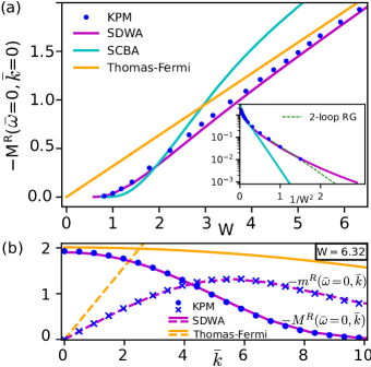
Figure 1: (a) Imaginary part of the disorder induced retarded self-energy for a 2d Dirac node at the nodal point as a function of disorder strength $W$. Our SDWA result (magenta line) compares well to the exact KPM data (blue dots) and asymptotically agrees with the Thomas-Fermi approximation (orange). The SCBA result is shown in cyan. Inset: For very small disorder, the SDWA deviates from the scaling found by RG (green dashed line). (b) The momentum dependence of the self-energy at $W=6.32$ calculated from KPM (blue symbols), the SDWA (magenta lines) and Thomas-Fermi approximation (orange lines).

Application to 2d Dirac node.—We now apply the SDWA to the case of a disordered 2d Dirac node, $H_{0}(\vec{k})=\hbar v(\sigma_{x}k_{x}+\sigma_{y}k_{y})$, with $E_{0}(k)=\hbar vk$ and the fundamental energy scale $E_{\xi}\!=\!\hbar v/\xi$. Using dimensionless variables $\vec{\bar{k}}\!=\!\vec{k}/\xi$ and $\bar{\omega}\!=\!\omega/E_{\xi}$, the ansatz for the self-energy reads

$$\Sigma(i\bar{\omega},\vec{\bar{k}})/E_{\xi}=m(\bar{\omega},\bar{k})[\sigma_{x}\cos\bar{\phi}+\sigma_{y}\sin\bar{\phi}]+iM(\bar{\omega},\bar{k}),$$ (4)

where we switched to polar coordinates for $\vec{\bar{k}}$ on the right hand side. While $m$ represents a renormalization of $H_{0}$, $M$ can be interpreted as a scattering rate. Using this ansatz in Eq. (3), we obtain two coupled ODEs:

$\displaystyle\partial_{\bar{\omega}}M(\bar{\omega},\bar{k})$ $\displaystyle=1\!+\!\frac{J_{0}(\bar{\omega},\bar{k})M(\bar{\omega},\bar{k})\!+\!J_{1}(\bar{\omega},\bar{k})m(\bar{\omega},\bar{k})}{W^{2}[J_{0}^{2}(\bar{\omega},\bar{k})+J_{1}^{2}(\bar{\omega},\bar{k})]},$ (5)
$\displaystyle\partial_{\bar{\omega}}m(\bar{\omega},\bar{k})$ $\displaystyle=\frac{J_{0}(\bar{\omega},\bar{k})m(\bar{\omega},\bar{k})-J_{1}(\bar{\omega},\bar{k})M(\bar{\omega},\bar{k})}{W^{2}[J_{0}^{2}(\bar{\omega},\bar{k})+J_{1}^{2}(\bar{\omega},\bar{k})]},$ (6)

where the functions $J_{0}$ and $J_{1}$ themselves depend on $m$ and $M$ as

$$\left\{\begin{array}[]{c}\!\!\!J_{0}(\bar{\omega},\bar{k})\!\!\!\\ \!\!\!J_{1}(\bar{\omega},\bar{k})\!\!\!\end{array}\right\}\!=\!\!\int_{0}^{\infty}\!\!\!\!d\bar{q}\left\{\begin{array}[]{c}\!\!\!\tilde{M}(\bar{\omega},\bar{q})I_{0}(\bar{k}\bar{q})\!\!\!\\ \!\!\!\tilde{m}(\bar{\omega},\bar{q})I_{1}(\bar{k}\bar{q})\!\!\!\end{array}\right\}\!\!\frac{\bar{q}e^{-(\bar{q}^{2}+\bar{k}^{2})/2}/(2\pi)}{\tilde{m}^{2}(\bar{\omega},\bar{q})\!+\!\tilde{M}^{2}(\bar{\omega},\bar{q})}.$$ (7)

Here, $I_{j}$ are modified Bessel functions of the first kind Gradshteyn and Ryzhik (2007), $\tilde{m}(\bar{\omega},\bar{k})\!=\!\bar{k}\!+\!m(\bar{\omega},\bar{k})$ and $\tilde{M}(\bar{\omega},\bar{k})\!=\!\bar{\omega}-\!M(\bar{\omega},\bar{k})$. The initial conditions for $\bar{\omega}_{max}\gg 1$ read $M(\bar{\omega}_{max},\bar{k})=-\frac{W^{2}}{2\pi\bar{\omega}_{max}}$ and $m(\bar{\omega}_{max},\bar{k})=0$.

The set of ODEs (5) and (6) can be solved numerically after discretizing the $\bar{k}$-dependence of $m$ and $M$ on a geometric grid. In Fig. 1(a) we compare the resulting disorder induced self-energy at the pole of the clean Green function, $M^{R}(\bar{\omega}=0,\bar{k}=0)=M(i\bar{\omega}=i\eta,\bar{k}=0)$ (magenta line) to the exact KPM data (blue dots), finding good agreement. This is true even for the smallest disorder strength $W\simeq 0.8$ that we can reach with KPM, see inset. Based on the above comment about the validity of SDWA, we consider this agreement for $M^{R}(\bar{\omega}=0,\bar{k}=0)\ll 1$ as coincidental. In fact the SDW solution for $M^{R}(\bar{\omega}=0,\bar{k}=0)$ does not agree asymptotically with the form $\sim\exp(-\pi/W^{2})/W$, that is inferred from the scale where the 2-loop Wilsonian RG-flow crosses over to strong disorder Schuessler et al. (2009) (green dashed line in the inset). In the supplemental material 222See Supplemental Material at [URL will be inserted by publisher] for a discussion of weak disorder in a 2d Dirac node, the Thomas-Fermi approximation for strong disorder, details on the SDWA for 3d Weyl and parabolic 2d semimetal and a derivation of the Schwinger-Dyson-Ward approximation we show additional KPM data confirming the validity of the RG result for weak disorder, albeit using a modified uncorrelated disorder model, where even smaller $M^{R}$ can be resolved.

In Fig. 1(a), we also illustrate the failure of the SCBA for all disorder strengths Aleiner and Efetov (2006); Ostrovsky et al. (2006) (cyan line). The data is obtained from an iterative numerical solution of the SCBA-equation, i.e. Eq. (3) without the derivative.

The momentum dependence of the self-energy at $W=6.32$ is addressed in Fig. 1(b). Again, the SDW results (dashed and solid magenta lines) compare well with exact KPM data (blue symbols). Note that $m^{R}(\bar{\omega}=0,\bar{k})\propto-\bar{k}$ encodes a velocity suppression.

In the limit of large disorder, $W\gg 1$, the typical electron wavelength (at zero total energy) is on the order of $\xi/W$, thus the electron motion in the disorder potential varying on the scale $\xi$ can be approximated as semi-classical Shklovskii and Efros (1984); Skinner (2014); Pesin et al. (2015). This motivates the Thomas-Fermi approximation, $G^{R}(\omega,\vec{k})=\int_{-\infty}^{\infty}dU\,P_{1}(U)[\omega+i\eta-H_{0}(\vec{k})-U]^{-1}$ where $P_{1}(U)=\exp\left(-\frac{U^{2}}{2\mathcal{K}(\vec{r}=0)}\right)/\sqrt{2\pi\mathcal{K}(\vec{r}=0)}$ is the distribution function of the disorder potential at a single point (see supplement Note (2) for details). At the nodal point, the Thomas-Fermi estimate Trappe et al. (2015); Volchkov et al. (2018) $M^{R}(\bar{\omega}\!=\!0,\bar{k}\!=\!0)E_{\xi}=-\frac{1}{\pi P_{1}(0)}$ agrees with the KPM and SDWA asymptotically [orange line in Fig. 1(a)]. Consequently, this result can also be reproduced analytically from Eq. (3) after setting $H_{0}\rightarrow 0$. However, for finite momentum, the Thomas-Fermi approximation fails even for strong disorder, see Fig. 1(b).

Refer to caption
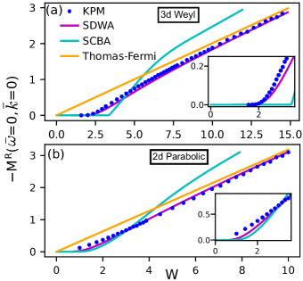
Figure 2: The same as in Fig. 1(a) but for (a) a 3d Weyl and (b) a 2d parabolic semimetal. The SDW results (magenta) compare well to the exact KPM data (blue) except for small $|M^{R}(\bar{\omega}=0,\bar{k}=0)|$, see insets.

Other dispersions.—To show the flexibility of the SDWA, we now modify the clean Hamiltonian $H_{0}$, modeling other types of nodal semimetals. First, we consider the case of a 3d Weyl node, $H_{0}(\vec{k})=\hbar v(\sigma_{x}k_{x}+\sigma_{y}k_{y}+\sigma_{z}k_{z})$, with $E_{0}$ and $E_{\xi}$ as before. The Weyl node features a disorder induced phase transition Fradkin (1986); Syzranov and Radzihovsky (2018), for $W$ below a critical disorder strength $W_{c}$, the self-energy vanishes at $k\!=\!0$. The ansatz for the self-energy and the resulting modifications to the ODEs (5) and (6) are detailed in the supplement Note (2). Fig. 2(a) compares the SDW results for $M^{R}(\bar{\omega}\!=\!0,\bar{k}\!=\!0)$ to KPM, SCBA and the Thomas-Fermi approximation. Again, while the SCBA fails quantitatively, our SDWA is in good agreement with the exact KPM data, except for small $|M^{R}(\bar{\omega}=0,\bar{k}=0)|$ (see inset). The Thomas-Fermi approximation clearly misses the phase transition but is valid asymptotically and we note Ref. Pesin et al. (2015) suggesting its systematic improvement for the 3d Weyl case, albeit for a different disorder model.

Second, we consider a 2d semimetal $H_{0}(\vec{k})=\frac{\hbar^{2}k^{2}}{m}\left[\sigma_{x}\cos(2\phi)+\sigma_{y}\sin(2\phi)\right]$ in polar coordinates. A similar Hamiltonian (with discrete rotation symmetry) occurs for Bernal-stacked bilayer graphene McCann and Koshino (2013). The dispersion is parabolic, $E_{0}(k)=\hbar^{2}k^{2}/m$ and we have $E_{\xi}=\hbar^{2}\xi^{-2}/m$ as the fundamental energy unit. The SDWA (see supplement Note (2) for details) yields good agreement to the KPM data, see Fig. 2(b), except in the small $|M^{R}(\bar{\omega}=0,\bar{k}=0)|$ regime below $W\simeq 2$.

Derivation of main result.—In the following, we sketch the main ideas behind Eq. (3). For a detailed derivation we refer to the supplemental material Note (2). Let $\mathrm{ln}\,\mathcal{Z}_{V}[\bar{\eta},\eta]$ be the generating functional for connected Green functions for a fixed disorder configuration $V$. The replica trick asserts that we can obtain the disorder averaged Green functions from the generating functional $\mathcal{Z}_{R}\left[\bar{\eta},\eta\right]=\left\langle\mathcal{Z}_{V}^{R}\left[\bar{\eta},\eta\right]\right\rangle_{dis}$ as $G_{12}=\underset{R\rightarrow 0}{\mathrm{lim}}\frac{1}{R}\frac{\delta^{2}\mathcal{Z}_{R}\left[\bar{\eta},\eta\right]}{\delta\bar{\eta}_{1}\delta\eta_{2}}|_{\eta,\bar{\eta}=0}$, where $\mathcal{Z}_{V}^{R}\left[\bar{\eta},\eta\right]$ contains $R$ replicated fermion species $\psi^{\alpha}$, $\alpha=1,2,...,R$, all coupling to the same disorder potential $V$ and the same source $\bar{\eta}$ (analogous for $\bar{\psi}^{\alpha}$ and $\eta$). We can now formally consider $\mathcal{Z}_{R}\left[\bar{\eta},\eta\right]\rightarrow\mathcal{Z}_{R}\left[\bar{\eta}^{\alpha},\eta^{\alpha},J\right]$ such that each fermion species couples to separate sources $\eta^{\alpha}$ and $\bar{\eta}^{\alpha}$ and introduce a source $J$ for the bosonic field $V$. Now, the Green function from Eq. (2) can be obtained as

$\displaystyle G_{12}$ $\displaystyle=\underset{R\rightarrow 0}{\mathrm{lim}}\frac{1}{R}\sum_{\alpha=1}^{R}G_{12}^{\alpha\alpha},\quad\!G_{12}^{\alpha\alpha}=\frac{\delta^{2}\mathcal{Z}_{R}\left[\bar{\eta}^{\alpha},\eta^{\alpha},J\right]}{\delta\bar{\eta}_{1}^{\alpha}\delta\eta_{2}^{\alpha}}\bigg{|}_{\bar{\eta},\eta,J=0},$ (8)

and likewise for the self-energy $\Sigma_{12}$, which is obtained as the second functional derivative of the generating functional of irreducible vertex functions Kopietz et al. (2010).

Next, we consider the Schwinger-Dyson equation for the self-energy, shown diagrammatically in Fig. 3(a). In the diagram, we already anticipate the replica limit that eliminates diagrammatic contributions with internal fermion loops Altland and Simons (2006). In this way a Hartree-like diagram, still present for $\Sigma^{\alpha\alpha}$, vanishes. Likewise, the bosonic self-energy, which contains internal fermion bubbles, is eliminated in the replica limit, such that the boson propagator $\mathcal{K}(\vec{q})$ is undressed (dashed line). Since $\mathcal{K}(\vec{q})$ is related to elastic scattering, no frequency is carried. The fermionic propagator in the loop on the right hand side does involve the fermionic self-energy from the left hand side. Finally, the triangle represents the Fermi-Bose vertex that, besides its bare part, subsumes the effect of all higher order diagrams with crossed impurity lines missing in the SCBA.

Refer to caption
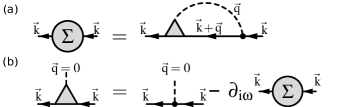
Figure 3: (a) Schwinger-Dyson equation for the fermionic self-energy $\Sigma$ and (b) the Ward-identity for the Fermi-Bose vertex (triangle). Together, they form the basis of the proposed SDWA. We suppress frequency and pseudo-spin indices.

In Fig. 3(b) we depict a Ward-identity for our theory $\mathcal{Z}_{R}$. It relates the Fermi-Bose vertex to the Matsubara frequency derivative of the fermionic self-energy. This relation follows from the invariance of the generating functional $\mathcal{Z}_{R}\left[\bar{\eta}^{\alpha},\eta^{\alpha},J\right]$ under a temporal gauge transformation $\psi_{\sigma}^{\alpha}(\tau,\vec{r})=e^{+iA_{\alpha}(\tau)}\psi_{\sigma}^{\prime\alpha}(\tau,\vec{r})$ and $\bar{\psi}_{\sigma}^{\alpha}(\tau,\vec{r})=e^{-iA_{\alpha}(\tau)}\bar{\psi}_{\sigma}^{\prime\alpha}(\tau,\vec{r})$. At an intermediate stage of the derivation, a bosonic Schwinger-Dyson equation (not shown) is used.

The idea is to eliminate the Fermi-Bose vertex in the Schwinger-Dyson equation (a) using the Ward-identity (b). Crucially, the Ward-identity requires vanishing bosonic momentum $\vec{q}=0$. Thus, in order to use (b) in (a), we need to approximate the Fermi-Bose vertex with its value at $\vec{q}\!=\!0$. Note that we keep $\vec{q}$ everywhere else in the diagram. This yields Eq. (3).

To motivate the above approximation, note that in the diagram of Fig. 3(a), we can restrict $|\vec{q}|=q\lesssim 1/\xi$ due to the finite range of the bosonic propagator $\mathcal{K}(\vec{q})\sim e^{-q^{2}\xi^{2}/2}$. We argue for the validity of the approximation on the basis of the standard self-consistent expansion of the disorder self-energy Bruus and Flensberg (2004), see Fig. 4(a). Comparing to the Schwinger-Dyson Eq. 3(a), we obtain the expansion of the Fermi-Bose vertex shown in Fig. 4(b). Alternatively, the expansion in Fig. 4(b) can be obtained from a Schwinger-Dyson equation for the Fermi-Bose vertex if the four-fermion vertex is treated perturbatively. The bare contribution is a constant and trivially $\vec{q}$-independent. The next contribution is a diagram with an internal boson line. The value of the internal (dressed) fermion propagators is dominant and nearly constant for momenta with magnitude $\lesssim 1/\gamma$, where $\gamma$ is the length-scale associated to disorder broadening of the pole; a finite Matsubara frequency $\omega>0$ only increases $\gamma$. Our approximation is valid in the regime $\gamma\lesssim\xi$, which means that the fermionic propagator with momentum $\vec{k}-\vec{p}+\vec{q}$ does not change once $\vec{q}$ is set to zero. It is plausible that this argument holds for all higher order diagrams although we cannot give a general proof. A priori, the relation between disorder strength $W$ and $\gamma$ is not clear, but the condition $\gamma\lesssim\xi$ can be checked from the result of the SDW approach a posteriori. Note however, that keeping the full momentum dependence of $G(\vec{k}+\vec{q})$ in the diagram of Fig. 3(a) is essential, setting $\vec{q}=0$ yields considerably worse results.

Refer to caption
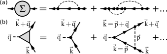
Figure 4: (a) Self-consistent perturbation theory for the disorder problem. The corresponding expansion of the Fermi-Bose vertex is shown in (b). Up to second order, it is used to argue for the validity of the $\vec{q}=0$ approximation in the limit of strong disorder. All internal fermion lines are self-energy dressed propagators.

Conclusion.—We presented a non-perturbative approach to calculate disorder averaged quasi-particle properties beyond SCBA. The SDWA for the self-energy requires a sufficient broadening of the quasiparticle pole to control the approximation involved. Systematic improvement is possible using a higher level truncation of the Schwinger-Dyson equations. This extended set may then be closed by Ward-identities. This should also allow for the calculation of conductivities. In contrast to the numerically expensive KPM, the analytical formulation of the SDW makes this method amenable for integration in other, possibly interacting, theories. For future work, one could try to the apply the SDWA to other types of disorder with non-trivial Pauli matrix structure Ostrovsky et al. (2006); Sbierski et al. (2016) or relax the particle-hole symmetry and isotropy assumption on the dispersion to study disordered tilted or anisotropic cones Trescher et al. (2015, 2017). The SDWA could also be useful for semimetals with a co-dimension of their Fermi-surface smaller than $d$, for example nodal-line semimetals in 3d Burkov et al. (2011).

Acknowledgments.—We thank Jörg Behrmann, Piet Brouwer, Christoph Karrasch, Georg Schwiete and Sergey Syzranov for useful discussions. Numerical computations were done on the HPC cluster of Fachbereich Physik at FU Berlin. Financial support was granted by the Deutsche Forschungsgemeinschaft through the Emmy Noether-program (KA 3360/2-1) and the CRC/Transregio 183 (Projects A02 and A03).

Supplemental material

for “Strong disorder in nodal semimetals: Schwinger-Dyson–Ward approach”

Weak disorder in 2d Dirac node

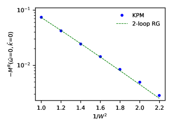
We now consider weak disorder in a 2d Dirac node. In Fig. 5 we prove by comparison to exact KPM data (blue dots) that the scaling $M^{R}(\bar{\omega}=0,\bar{k}=0)\sim W^{-1}\exp(-\pi/W^{2})$ inferred from the 2-loop momentum shell RG flow equation Schuessler et al. (2009) is correct (green dashed line). This result is obtained from the scale where the RG-flow crosses over to strong disorder. To the best of our knowledge, this scaling has never been checked numerically. Note that the RG uses a white-noise disorder correlator which cannot be implemented numerically and is responsible for the $\sim$ sign above. To obtain converged values of small $M^{R}$ over two orders of magnitude, we chose a discrete disorder model where the “correlation length” $\xi$ equals the real-space lattice constant $a$, such that the disorder correlator $\xi=a$ is not smooth on the lattice scale. Thus, the SDWA formulated for the field-theory limit $\xi\gg a$ is not directly applicable. The potential at each site of the real-space lattice is uniformly distributed, $V(\vec{r})\in[-\sqrt{3}W,\sqrt{3}W]$. This yields $\sum_{\vec{r}}\left\langle V(\vec{r})V(\vec{0})\right\rangle_{dis}=\frac{1}{2\sqrt{3}W}\int_{-\sqrt{3}W}^{+\sqrt{3}W}dU\,U^{2}=W^{2}$. We use $P=2^{12}$ lattice points in both linear directions, such that $a=\frac{2\pi}{P\Delta k}$ and $60000$ moments for convergence of the KPM. We checked that the disorder induced energy scale $M^{R}(\bar{\omega}=0,\bar{k}=0)\hbar v/a$ is always larger than the finite-size energy scale $E_{fs}=\hbar v\Delta k$.

Refer to caption
Figure 5: Imaginary part of the disorder induced retarded self-energy for a 2d Dirac node with discrete disorder as a function of disorder strength $W$. The exact KPM data is shown as blue dots, the RG prediction $M^{R}\sim W^{-1}\exp(-\pi/W^{2})$ with an appropriate prefactor fitted is shown as a green dashed line.

Thomas-Fermi approximation for strong disorder

The Thomas-Fermi approximation Pesin et al. (2015); Shklovskii and Efros (1984) amounts to approximate the disorder potential as a homogeneous effective chemical potential term. Then, the disorder averaged Green function is approximated as

$$G^{R}(\omega,\vec{k})=\int_{-\infty}^{\infty}dU\,P_{1}(U)\frac{1}{\omega+i\eta-H_{0}(\vec{k})-U},$$ (9)

where $P_{1}(U)$ is the one-point distribution function, i.e. the probability that the local potential $V(\vec{r}_{1})$ has the value $U$. This probability can be obtained as the expectation value $P_{1}(U)=\left\langle\delta\left(V(\vec{r}_{1})-U\right)\right\rangle_{dis}$ which can be calculated by representing the $\delta$-function as an integral over an exponential and subsequently employing the rules for functional integration over $V$. The result is

$\displaystyle P_{1}(U)$ $\displaystyle=$ $\displaystyle\left\langle\frac{1}{2\pi}\int_{-\infty}^{+\infty}dx\,e^{i\left(V(\vec{r}_{1})-U\right)x}\right\rangle_{dis}=\frac{1}{2\pi}\int_{-\infty}^{+\infty}dx\,e^{-\frac{1}{2}x^{2}\left\langle V^{2}(\vec{r}_{1})\right\rangle_{dis}-iUx}=\frac{1}{\sqrt{2\pi\mathcal{K}(\vec{0})}}e^{-\frac{U^{2}}{2\mathcal{K}(\vec{0})}},$ (10)

where $\mathcal{K}(\vec{0})=\left\langle V^{2}(\vec{r}_{1})\right\rangle_{dis}=(2\pi)^{-d/2}W^{2}E_{\xi}^{2}$.

We evaluate Eq. (9) for the 2d Dirac case in the helicity basis at $\omega=0$ and find

$\displaystyle G_{\lambda,\lambda^{\prime}}^{R}(\bar{\omega}=0,\bar{k})E_{\xi}$ $\displaystyle=$ $\displaystyle-\delta_{\lambda,\lambda^{\prime}}\frac{\pi}{W}\left(\text{erfi}\left(\frac{\lambda\bar{k}}{\sqrt{\pi}W}\right)+i\right)e^{-(\bar{k})^{2}/(\pi W^{2})}.$ (11)

Here, $\text{erfi}(z)$ is the imaginary error function defined as $\text{erfi}(z)=\text{erf}(iz)/i$ Gradshteyn and Ryzhik (2007). With the ansatz

$$G_{\lambda,\lambda^{\prime}}^{R}(\bar{\omega}=0,\bar{k})E_{\xi}=\frac{\delta_{\lambda,\lambda^{\prime}}}{-\lambda\left[\bar{k}+m^{R}(\bar{\omega}=0,\bar{k})\right]-iM^{R}(\bar{\omega}=0,\bar{k})},$$ (12)

we obtain

$\displaystyle M^{R}(\bar{\omega}=0,\bar{k})$ $\displaystyle=$ $\displaystyle-\frac{W}{\pi}\frac{e^{\bar{k}^{2}/(\pi w^{2})}}{\text{erfi}^{2}\left(\frac{\bar{k}}{\sqrt{\pi}W}\right)+1}=-\frac{W}{\pi}+\frac{(4-\pi)\bar{k}^{2}}{W\pi^{3}}+\mathcal{O}(\bar{k}^{3}),$ (13)
$\displaystyle m^{R}(\bar{\omega}=0,\bar{k})$ $\displaystyle=$ $\displaystyle-\bar{k}+\frac{W}{\pi}\frac{e^{\bar{k}^{2}/(\pi w^{2})}\text{erfi}\left(\frac{\bar{k}}{\sqrt{\pi}W}\right)}{\text{erfi}^{2}\left(\frac{\bar{k}}{\sqrt{\pi}W}\right)+1}=-\underset{\simeq 0.8}{\underbrace{(1-2/\pi^{2})}}\bar{k}+\mathcal{O}(\bar{k}^{2}).$ (14)

Details on the SDWA for 3d Weyl and parabolic 2d semimetal

For the 3d Weyl node with $H_{0}(\vec{k})=\hbar v(\sigma_{x}k_{x}+\sigma_{y}k_{y}+\sigma_{z}k_{z})$ we consider the self-energy ansatz

$\displaystyle\Sigma(\vec{k},i\omega)/E_{\xi}=$ $\displaystyle m(\bar{\omega},\bar{k})\left[\sin\bar{\theta}\left(\sigma_{x}\cos\bar{\phi}+\sigma_{y}\sin\bar{\phi}\right)+\sigma_{z}\cos\bar{\theta}\right]+iM(\bar{\omega},\bar{k}).$ (15)

Upon insertion into Eq. (3) we find that Eqs. (5) and (6) remain valid, but with the replacements $\{J_{0},J_{1}\}$ $\rightarrow$ $\{J_{0}^{w},J_{1}^{w}\}$ where

$\displaystyle\left\{\begin{array}[]{c}\!J_{0}^{w}(\bar{\omega},\bar{k})\!\\ \!J_{1}^{w}(\bar{\omega},\bar{k})\!\end{array}\right\}=$ $\displaystyle\!\int_{0}^{\infty}\!\!d\bar{q}\left\{\begin{array}[]{c}\bar{k}\bar{q}\sinh(\bar{k}\bar{q})\tilde{M}(\bar{\omega},\bar{q})\\ \!\!\left[\bar{k}\bar{q}\cosh(\bar{k}\bar{q})-\sinh(\bar{k}\bar{q})\right]\tilde{m}(\bar{\omega},\bar{q})\!\!\end{array}\right\}\frac{e^{-(\bar{q}^{2}+\bar{k}^{2})/2}/(2\pi^{2}\bar{k}^{2})}{\tilde{m}^{2}(\bar{\omega},\bar{q})+\tilde{M}^{2}(\bar{\omega},\bar{q})}.$ (20)

In addition, the initial conditions are modified to $M(\bar{\omega}_{max},\bar{k})=-W^{2}(2\pi)^{-3/2}/\bar{\omega}_{max}$ and $m(\bar{\omega}_{max},\bar{k})=0$.

For the 2d parabolic semimetal, described by the clean Hamiltonian $H_{0}(\vec{k})=\frac{\hbar^{2}k^{2}}{m}\left[\sigma_{x}\cos(2\phi)+\sigma_{y}\sin(2\phi)\right]$ we use the self-energy ansatz

$$\Sigma(\vec{k},i\omega)/E_{\xi}=m(\bar{\omega},\bar{k})\left[\sigma_{x}\cos(2\bar{\phi})+\sigma_{y}\sin(2\bar{\phi})\right]+iM(\bar{\omega},\bar{k}).$$ (21)

We arrive at Eqs. (5) and (6) with the redefinition $\tilde{m}(\bar{\omega},\bar{k})=\bar{k}^{2}+m(\bar{\omega},\bar{k})$ and the replacements $\{J_{0},J_{1}\}$ $\rightarrow$ $\{J_{0}^{p},J_{1}^{p}\}$, where

$$\left\{\begin{array}[]{c}\!J_{0}^{p}(\bar{\omega},\bar{k})\!\\ \!J_{1}^{p}(\bar{\omega},\bar{k})\!\end{array}\right\}\!=\!\int_{0}^{\infty}\!\!d\bar{q}\left\{\begin{array}[]{c}\!\!\tilde{M}(\bar{\omega},\bar{q})I_{0}(\bar{k}\bar{q})\!\!\\ \!\!\tilde{m}(\bar{\omega},\bar{q})I_{2}(\bar{k}\bar{q})\!\!\end{array}\right\}\frac{\bar{q}e^{-(\bar{q}^{2}+\bar{k}^{2})/2}/(2\pi)}{\tilde{m}^{2}(\bar{\omega},\bar{q})+\tilde{M}^{2}(\bar{\omega},\bar{q})}.$$ (22)

The initial conditions are the same as in the 2d Dirac case, $M(\bar{\omega}_{max},\bar{k})=-\frac{W^{2}}{2\pi\bar{\omega}_{max}}$ and $m(\bar{\omega}_{max},\bar{k})=0$.

Detailed derivation of the Schwinger-Dyson-Ward approximation

Within the following derivation, we mostly stick to the conventions and definitions of Ref. Kopietz et al. (2010).

.1 Preliminaries

For a given disorder realization $V(\vec{r})$, the generating functional for fermionic imaginary-time Green functions is given by

$$\mathcal{Z}_{V}\left[\bar{\eta},\eta\right]=\int\mathcal{D}\bar{\psi}\,\mathcal{D}\psi\,e^{-S_{V}\left[\bar{\psi},\psi\right]+(\bar{\eta},\psi)+(\bar{\psi},\eta)},$$ (23)

where $S_{V}\left[\bar{\psi},\psi\right]$ is the Euclidean action of the system in the presence of the disorder field $V$

$$S_{V}\left[\bar{\psi},\psi\right]=S_{0}\left[\bar{\psi},\psi\right]+\sum_{\sigma}\int_{\vec{r},\tau}\bar{\psi}_{\sigma}\left(\vec{r},\tau\right)V\left(\vec{r}\right)\psi_{\sigma}\left(\vec{r},\tau\right).$$ (24)

The index $\sigma$ plays the role of a pseudo-spin, which is necessary to describe a two band model. Its clean part, $S_{0}\left[\bar{\psi},\psi\right]$, derives from the Hamiltonian $H_{0}(\vec{k}=-i\hbar\vec{\nabla})$ as follows Negele and Orland (1988); Altland and Simons (2006)

$$S_{0}\left[\bar{\psi},\psi\right]=\sum_{\sigma\sigma^{\prime}}\int_{\vec{r},\tau}\bar{\psi}_{\sigma}\left(\vec{r},\tau\right)\left[\partial_{\tau}+H_{0}(-i\hbar\vec{\nabla})\right]_{\sigma\sigma^{\prime}}\psi_{\sigma^{\prime}}\left(\vec{r},\tau\right).$$ (25)

For the source terms, involving the Grassmann-valued fields $\eta$ and $\bar{\eta}$, we used the compact scalar product notation $(\bar{\psi},\eta)\equiv\sum_{\sigma}\int_{\vec{r},\tau}\bar{\psi}_{\sigma}\left(\vec{r},\tau\right)\eta_{\sigma}\left(\vec{r},\tau\right)$. The $n$-point Green functions at a fixed disorder field configuration can then be obtained as an $n$-fold functional derivative of $\mathcal{Z}_{V}$ with respect to the sources. For the two-point Green function, for example, we have

$$G_{V,\sigma\sigma^{\prime}}\left(\vec{r},\tau;\vec{r}^{\prime},\tau^{\prime}\right)=-\left\langle\psi_{\sigma}(\vec{r},\tau)\bar{\psi}_{\sigma^{\prime}}(\vec{r}^{\prime},\tau^{\prime})\right\rangle=\frac{1}{\mathcal{Z}_{V}[0,0]}\frac{\delta^{2}\mathcal{Z}_{V}\left[\bar{\eta},\eta\right]}{\delta\bar{\eta}_{\sigma}(\vec{r},\tau)\,\delta\eta_{\sigma^{\prime}}(\vec{r}^{\prime},\tau^{\prime})}\bigg{|}_{\eta=\bar{\eta}=0}.$$ (26)

Note the appearance of the $V$-dependent normalization $\mathcal{Z}_{V}[0,0]$. The connected $n$-point Green functions at fixed disorder configuration are defined as the $n$-fold derivative of the connected functional $\mathcal{G}_{V}\left[\bar{\eta},\eta\right]=\ln\mathcal{Z}_{V}\left[\bar{\eta},\eta\right]$, just as usual. Since our theory is non-interacting, the only non-vanishing connected correlator is the two-point function (26).

Since we are not interested in one particular disorder realization, but in a statistical ensemble of disorder potentials, we have to perform an ensemble average. To this end, one has to specify the statistical properties of the ensemble, which are summarized in a probability distribution $P[V]$. Here, we choose the Gaussian probability distribution

$$P\left[V\right]=\mathcal{N}\exp\left(-\frac{1}{2}\int_{\vec{r},\vec{r}^{\prime}}V(\vec{r})\mathcal{K}^{-1}(\vec{r}-\vec{r}^{\prime})V(\vec{r}^{\prime})\right),$$ (27)

where $\mathcal{K}^{-1}\left(\vec{r}-\vec{r}^{\prime}\right)$ is the distributional inverse of the fundamental disorder correlator $\left\langle V(\vec{r})V(\vec{r}^{\prime})\right\rangle_{dis}=\mathcal{K}\left(\vec{r}-\vec{r}^{\prime}\right)$, and $\mathcal{N}$ is a normalization constant. The disorder average of a general quantity $Q[V]$ is then defined as $\left\langle Q\right\rangle_{dis}=\int\mathcal{D}VQ[V]P[V]$. To obtain disorder averaged correlation functions one would have to either average each $n$-point function individually, or average the normalized generating functional (23), that is $\left\langle\mathcal{Z}_{V}[\bar{\eta},\eta]/\mathcal{Z}_{V}[0,0]\right\rangle_{dis}$, which would serve as the generating functional of disorder averaged Green functions. However, due to the $V$-dependent normalization $\mathcal{Z}_{V}[0,0]$ in the denominator, it is not possible to naively perform the disorder average.

To circumvent this problem and get rid of the denominator there are three possibilities Altland and Simons (2006): (1) work in real time using the Keldysh technique; (2) rewrite the denominator as a bosonic Gaussian integral, a technique known as supersymmetry method; or (3) “replicate the system” and perform an analytical continuation to zero replicas at the end. Here, we choose the latter option. The trick is to rewrite the connected functional $\mathcal{G}_{V}\left[\bar{\eta},\eta\right]$ as follows

$$\mathcal{G}_{V}\left[\bar{\eta},\eta\right]=\ln\mathcal{Z}_{V}\left[\bar{\eta},\eta\right]=\underset{R\rightarrow 0}{\mathrm{lim}}\frac{1}{R}\left(e^{R\ln\mathcal{Z}_{V}\left[\bar{\eta},\eta\right]}-1\right)=\underset{R\rightarrow 0}{\mathrm{lim}}\frac{1}{R}\left(\mathcal{Z}_{V}^{R}\left[\bar{\eta},\eta\right]-1\right),$$ (28)

which allows us to perform the disorder average. The disorder averaged replicated partition function then reads

$\displaystyle\mathcal{Z}_{R}\left[\bar{\eta},\eta\right]$ $\displaystyle\equiv\left\langle\mathcal{Z}_{V}^{R}\left[\bar{\eta},\eta\right]\right\rangle_{dis}$
$\displaystyle=\int\mathcal{D}\bar{\psi}^{\alpha}\,\mathcal{D}\psi^{\alpha}\,\mathcal{D}V\exp\left(-S_{R}[\bar{\psi}^{\alpha},\psi^{\alpha},V]+\sum_{\alpha=1}^{R}(\bar{\eta},\psi^{\alpha})+\sum_{\alpha=1}^{R}(\bar{\psi}^{\alpha},\eta)\right),$ (29)

with the replicated action $S_{R}[\bar{\psi}^{\alpha},\psi^{\alpha},V]\equiv\sum_{\alpha=1}^{R}S_{V}[\bar{\psi}^{\alpha},\psi^{\alpha}]+\frac{1}{2}\int_{\vec{r},\vec{r}^{\prime}}V(\vec{r})\mathcal{K}^{-1}(\vec{r}-\vec{r}^{\prime})V(\vec{r}^{\prime})$. Note that there is only a single source for all replicas and only a single disorder potential coupling identically to the replica bilinears in $S_{V}[\bar{\psi}^{\alpha},\psi^{\alpha}]$. In the standard treatment one would integrate out the disorder field to obtain a quartic pseudo-interaction term for the fermions Altland and Simons (2006), but here we take another path. Instead of performing the bosonic Gaussian integral, we consider a generalization of Eq. (29), where a bosonic source $J$ coupling to $V$ is introduced and where the fermionic sources now carry a replica index as well

$$\mathcal{Z}_{R}\left[\bar{\eta},\eta\right]\rightarrow\mathcal{Z}_{R}\left[\bar{\eta}^{\alpha},\eta^{\alpha},J\right]=\int\mathcal{D}\bar{\psi}^{\alpha}\,\mathcal{D}\psi^{\alpha}\,\mathcal{D}V\exp\left(-S_{R}\left[\bar{\psi}^{\alpha},\psi^{\alpha},V\right]+\sum_{\alpha=1}^{R}(\bar{\eta}^{\alpha},\psi^{\alpha})+\sum_{\alpha=1}^{R}(\bar{\psi}^{\alpha},\eta^{\alpha})+(J,V)\right).$$ (30)

Introducing the super-field vector $\boldsymbol{\Phi}=(\psi^{\alpha},\bar{\psi}^{\alpha},V)$, the super-source vector $\mathbf{J}=\left(\bar{\eta}^{\alpha},-\eta^{\alpha},J\right)$, and the scalar product $(\mathbf{J},\boldsymbol{\Phi})=\sum_{\alpha=1}^{R}(\bar{\eta}^{\alpha},\psi^{\alpha})+\sum_{\alpha=1}^{R}(\bar{\psi}^{\alpha},\eta^{\alpha})+(J,V)$, we can write this new functional in the compact form $\mathcal{Z}_{R}\left[\mathbf{J}\right]\equiv\int\mathcal{D}\boldsymbol{\Phi}\exp\left(-S_{R}\left[\boldsymbol{\Phi}\right]+(\mathbf{J},\boldsymbol{\Phi})\right)$. Putting everything together we find the disorder averaged connected Green function

GV,12dis=δ2ln𝒵V[η¯,η]δη¯1δη2|η¯=η=0dis=(28)(30)limR01Rα=1Rδ2𝒵R[𝐉]δη¯1αδη2α|𝐉=0limR01Rα=1RG12αα.subscriptdelimited-⟨⟩subscript𝐺𝑉12𝑑𝑖𝑠evaluated-atsubscriptdelimited-⟨⟩evaluated-atsuperscript𝛿2subscript𝒵𝑉¯𝜂𝜂𝛿subscript¯𝜂1𝛿subscript𝜂2¯𝜂𝜂0𝑑𝑖𝑠italic-(28italic-)italic-(30italic-)𝑅0lim1𝑅superscriptsubscript𝛼1𝑅superscript𝛿2subscript𝒵𝑅delimited-[]𝐉𝛿superscriptsubscript¯𝜂1𝛼𝛿superscriptsubscript𝜂2𝛼𝐉0𝑅0lim1𝑅superscriptsubscript𝛼1𝑅superscriptsubscript𝐺12𝛼𝛼\left\langle G_{V,12}\right\rangle_{dis}=\left\langle\frac{\delta^{2}\ln\mathcal{Z}_{V}\left[\bar{\eta},\eta\right]}{\delta\bar{\eta}_{1}\delta\eta_{2}}\bigg{|}_{\bar{\eta}=\eta=0}\right\rangle_{dis}\overset{\eqref{eq:replica}-\eqref{eq:GeneralizedZR}}{=}\underset{R\rightarrow 0}{\mathrm{lim}}\frac{1}{R}\sum_{\alpha=1}^{R}\frac{\delta^{2}\mathcal{Z}_{R}\left[\mathbf{J}\right]}{\delta\bar{\eta}_{1}^{\alpha}\delta\eta_{2}^{\alpha}}\bigg{|}_{\mathbf{J}=0}\equiv\underset{R\rightarrow 0}{\mathrm{lim}}\frac{1}{R}\sum_{\alpha=1}^{R}G_{12}^{\alpha\alpha}. (31)

Here, the numerical indices 1 and 2 are a compact notation, which include space, imaginary-time and pseudo-spin indices. In the following we consider a finite number of replicas $R$ – the replica limit will only be taken at the end of the calculation – and compute $G_{12}^{\alpha\alpha}=\frac{\delta^{2}\mathcal{Z}_{R}\left[\mathbf{J}\right]}{\delta\bar{\eta}_{1}^{\alpha}\delta\eta_{2}^{\alpha}}\big{|}_{\mathbf{J}=0}=-\left\langle\psi_{1}^{\alpha}\bar{\psi}_{2}^{\alpha}\right\rangle_{S_{R}}$. The subscript at the average is just a reminder that it has to be performed with respect to the replicated action $S_{R}$ in Eq. (30).

.2 Schwinger-Dyson equations

As is well-known, in classical field theory the equations of motions follow from a least action principle. Its generalization to quantum field theories and the corresponding quantum equations of motion follow from a functional analog of the fundamental theorem of calculus, stating that the functional integral over a total derivative vanishes Peskin and Schröder (1995); Kopietz et al. (2010)

$\displaystyle 0=\int\mathcal{D}\boldsymbol{\Phi}\frac{\delta}{\delta\boldsymbol{\Phi}_{i}}e^{-S_{R}\left[\boldsymbol{\Phi}\right]+(\mathbf{J},\boldsymbol{\Phi})}=\int\mathcal{D}\boldsymbol{\Phi}\left(-\frac{\delta S_{R}}{\delta\boldsymbol{\Phi}_{i}}+\boldsymbol{\zeta}_{i}\boldsymbol{J}_{i}\right)e^{-S_{R}\left[\boldsymbol{\Phi}\right]+(\mathbf{J},\boldsymbol{\Phi})}\equiv\left\langle-\frac{\delta S_{R}}{\delta\boldsymbol{\Phi}_{i}}+\boldsymbol{\zeta}_{i}\boldsymbol{J}_{i}\right\rangle_{\mathbf{J}}.$ (32)

Here, the index $i$ encompasses space, imaginary time, the discrete pseudo-spin index as well as the super-field component, see our definition above. Furthermore, $\boldsymbol{\zeta}_{i}$ is a statistical factor, which is $-1$ for a fermionic source and $+1$ for a bosonic one, and the subscript $\mathbf{J}$ at the functional average indicates that it has to be performed in the presence of the source fields. We can rewrite these expectation values as functional differential equations by replacing the $\boldsymbol{\Phi}$-dependence of $\frac{\delta S_{R}}{\delta\boldsymbol{\Phi}_{i}}$ with their corresponding source-derivatives

$$\left(-\frac{\delta S_{R}}{\delta\boldsymbol{\Phi}_{i}}\left[\frac{\delta}{\delta\mathbf{J}}\right]+\boldsymbol{\zeta}_{i}\boldsymbol{J}_{i}\right)\mathcal{Z}_{R}\left[\mathbf{J}\right]=0.$$ (33)

This set of equations is known as Schwinger-Dyson equations and they serve as master equations, which can be functionally differentiated to obtain an infinite hierarchy of coupled integral equations for the one-particle irreducible vertex functions.

To obtain such equations one has to switch to the connected functional $\mathcal{G}_{R}[\mathbf{J}]=\ln\mathcal{Z}_{R}[\mathbf{J}]$, and perform a Legendre transformation to the effective action $\mathcal{L}_{R}[\mathbf{\Phi}]=-\mathcal{G}_{R}[\mathbf{J}]+(\mathbf{J},\mathbf{\Phi})$. Here, the super-field vector $\mathbf{\Phi}$ is the quantum expectation value $\mathbf{\Phi}=\frac{\delta\mathcal{G}_{R}[\mathbf{J}]}{\delta\mathbf{J}}$ in the presence of the source fields $\mathbf{J}$. It shall not be confused with the integration variables in Eqs. (30) and (32). Following Ref. Kopietz et al. (2010), we write $\mathcal{L}_{R}[\mathbf{\Phi}]=S_{0}[\mathbf{\Phi}]+\Gamma_{R}[\mathbf{\Phi}]$, where $S_{0}[\mathbf{\Phi}]\equiv\sum_{\alpha=1}^{R}S_{V=0}[\bar{\psi}^{\alpha},\psi^{\alpha}]+\frac{1}{2}\int_{\vec{r},\vec{r}^{\prime}}V(\vec{r})\mathcal{K}^{-1}(\vec{r}-\vec{r}^{\prime})V(\vec{r}^{\prime})$ is the bare quadratic action and $\Gamma_{R}[\mathbf{\Phi}]$ is the generating functional of one-particle irreducible vertex functions, or vertex functional for short. As a result, we find the Schwinger-Dyson equations in the form

$\displaystyle\frac{\delta\Gamma_{R}[\mathbf{\Phi}]}{\delta\bar{\psi}_{\sigma}^{\alpha}(\vec{r},\tau)}$ $\displaystyle=V(\vec{r})\psi_{\sigma}^{\alpha}(\vec{r},\tau)+\frac{\delta^{2}\mathcal{G}_{R}[\mathbf{J}]}{\delta J(\vec{r})\delta\bar{\eta}_{\sigma}^{\alpha}(\vec{r},\tau)},$ (34)
$\displaystyle\frac{\delta\Gamma_{R}[\mathbf{\Phi}]}{\delta\psi_{\sigma}^{\alpha}(\vec{r},\tau)}$ $\displaystyle=-\bar{\psi}_{\sigma}^{\alpha}(\vec{r},\tau)V(\vec{r})+\frac{\delta^{2}\mathcal{G}_{R}[\mathbf{J}]}{\delta\eta_{\sigma}^{\alpha}(\vec{r},\tau)\delta J(\vec{r})},$ (35)
$\displaystyle\frac{\delta\Gamma_{R}[\mathbf{\Phi}]}{\delta V(\vec{r})}$ $\displaystyle=\sum_{\alpha=1}^{R}\sum_{\sigma}\int_{\tau}\bar{\psi}_{\sigma}^{\alpha}(\vec{r},\tau)\psi_{\sigma}^{\alpha}(\vec{r},\tau)-\sum_{\alpha=1}^{R}\sum_{\sigma}\int_{\tau}\frac{\delta^{2}\mathcal{G}_{R}[\mathbf{J}]}{\delta\eta_{\sigma}^{\alpha}(\vec{r},\tau)\delta\bar{\eta}_{\sigma}^{\alpha}(\vec{r},\tau)}.$ (36)

On the right hand side, the second functional derivatives of $\mathcal{G}_{R}$ still have to be replaced by second functional derivatives of $\Gamma_{R}$, using the inversion relation between the Hesse matrices of $\mathcal{G}_{R}$ and $\mathcal{L}_{R}$, see Refs. Negele and Orland (1988); Kopietz et al. (2010). This substitution eliminates the remaining source field dependence, but it leads to rather complex expressions. For this reason we leave the above equations in this compact mixed form. To obtain the infinite hierarchy of integral equations for the one-particle irreducible vertex functions as advertised above, one has to expand the vertex functional $\Gamma_{R}$ in a Taylor series in terms of fields, insert the expression on the left and right hand sides and compare coefficients. Alternatively one may simply apply a corresponding amount of field derivatives $\frac{\delta}{\delta\mathbf{\Phi}}$ to the above set of equations and set the sources $\mathbf{J}$ to zero afterwards. When the sources $\mathbf{J}$ are set to zero, the fields in $\Gamma_{R}$ are set to their possibly finite expectation value $\mathbf{\Phi_{c}}=\mathbf{\Phi}|_{\mathbf{J}=0}=\frac{\delta\mathcal{G}[\mathbf{J}]}{\delta\mathbf{J}}\big{|}_{\mathbf{J}=0}$ Kopietz et al. (2010). (In the present case only the bosonic field may develop a finite expectation value.) In the Taylor expansion of $\Gamma_{R}$ one should account for that fact by expanding around $\mathbf{\Phi}=\mathbf{\Phi_{c}}$, instead of $\mathbf{\Phi}=0$, such that the vertex functions are defined as field-derivatives of $\Gamma_{R}$ evaluated at $\mathbf{\Phi}=\mathbf{\Phi_{c}}$.

The Schwinger-Dyson equation for the fermionic self-energy, which is defined by $\Sigma_{12}=-\delta^{2}\Gamma_{R}/\delta\bar{\psi}_{1}\delta\psi_{2}|_{\mathbf{\Phi}=\mathbf{\Phi_{c}}}$, may be obtained from Eq. (34) after applying the derivative $\frac{\delta}{\delta\psi}$. A short calculation yields the following equation in Fourier space

$\displaystyle\Sigma_{\sigma_{1}\sigma_{2}}^{\alpha\alpha}\left(i\omega,\vec{k}\right)$ $\displaystyle=\delta_{\sigma_{1},\sigma_{2}}\mathcal{K}(0)\sum_{\beta=1}^{R}\sum_{\sigma}\int_{\vec{k}^{\prime},\omega^{\prime}}G_{\sigma\sigma}^{\beta\beta}(i\omega^{\prime},\vec{k}^{\prime})$
$\displaystyle-\sum_{\sigma}\int_{\vec{q}}F\left(\vec{q}\right)\frac{\delta^{3}\Gamma}{\delta\bar{\psi}_{\sigma_{1}}^{\alpha}(i\omega,\vec{k})\delta\psi_{\sigma}^{\alpha}(i\omega,\vec{k}+\vec{q})\delta V(-\vec{q})}\bigg{|}_{\mathbf{\Phi}=\mathbf{\Phi}_{c}}G_{\sigma\sigma_{2}}^{\alpha\alpha}(i\omega,\vec{k}+\vec{q}),$ (37)

with $\int_{\vec{q}}=\int\frac{d^{d}q}{(2\pi)^{d}}$. The term in the first line, involving a closed fermion loop and the bare disorder propagator at vanishing momentum, is the Hartree contribution to the self-energy. It represents the influence of a finite expectation value of $V$ on the fermions, and has been obtained by employing Eq. (36) at $\mathbf{J}=0$. The term in the second line represents the Fock exchange self-energy, where the third derivative of $\Gamma_{R}$ is the full Fermi-Bose three vertex. Furthermore, $G_{\sigma_{1}\sigma_{2}}^{\alpha\alpha}(i\omega,\vec{k})$ and $F\left(\vec{q}\right)$ are the full fermionic and bosonic propagators, respectively. The former involves the fermionic self-energy, which makes Eq. (37) a self-consistency equation, while the latter involves the bosonic self-energy – polarization bubbles, for which there exists a separate equation, that derives from Eq. (36) after applying $\frac{\delta}{\delta V}$. We emphasize that the closed fermion loops in the Hartree term and the polarization bubbles are finite prior to taking the replica limit. They only vanish in the replica limit, which we will discuss at the end, see Sec. .4. Anticipating the replica limit, Eq. (37) is depicted in Fig. 3(a).

.3 Ward identity

According to Noether’s theorem a continuous symmetry in a classical field theory leads to conservation laws. In a quantum field theory such symmetries lead to Ward identities, which connect various vertex functions to one another Kopietz et al. (2010). In the present case the fermions obey a global $U(1)^{\otimes R}$ symmetry, which formally expresses the fact that the particle number for each replica is conserved. To obtain a relation between different correlation functions we have to consider a local $U(1)^{\otimes R}$ symmetry transformation

$$\psi_{\sigma}^{\alpha}(\tau,\vec{r})=e^{+iA^{\alpha}(\tau)}\psi_{\sigma}^{\prime\alpha}(\tau,\vec{r}),\quad\bar{\psi}_{\sigma}^{\alpha}(\tau,\vec{r})=\bar{\psi}_{\sigma}^{\prime\alpha}(\tau,\vec{r})e^{-iA^{\alpha}(\tau)}.$$ (38)

(Here, we took the phase field $A^{\alpha}$ to be local in imaginary time only. Spatial locality is not relevant, but could be incorporated without problems.) This transformation leads to an additional term in the action,

$$S_{R}\left[\bar{\psi}^{\alpha},\psi^{\alpha},V\right]=S_{R}\left[\bar{\psi}^{\prime\alpha},\psi^{\prime\alpha},V\right]+\sum_{\sigma}\int_{\vec{r},\tau}\bar{\psi}_{\sigma}^{\prime\alpha}(\tau,\vec{r})\left\{\partial_{\tau}iA^{\alpha}(\tau,\vec{r})\right\}\psi_{\sigma}^{\prime\alpha}(\tau,\vec{r}),$$ (39)

but it leaves the functional integral measure and the partition function itself invariant. As a consequence of the latter fact we obtain the following relation

$$0=\int\mathcal{D}\mathbf{\Phi}\left(e^{(\bar{\eta},\psi)+(\bar{\psi},\eta)}-e^{-\sum_{\sigma}\int_{\vec{r},\tau}\bar{\psi}_{\sigma}^{\alpha}(\tau,\vec{r})\big{\{}\partial_{\tau}iA^{\alpha}(\tau,\vec{r})\big{\}}\psi_{\sigma}^{\alpha}(\tau,\vec{r})+\left(\bar{\eta},e^{iA}\psi\right)+\left(\bar{\psi}e^{-iA},\eta\right)}\right)e^{-S_{R}[\mathbf{\Phi}]+(J,V)}.$$ (40)

Considering only an infinitesimal phase transformation this identity becomes

$$0=\left\langle\sum_{\alpha=1}^{R}\sum_{\sigma}\int_{\vec{r},\tau}\Big{(}-\bar{\psi}_{\sigma}^{\alpha}(\tau,\vec{r})\big{\{}\partial_{\tau}A^{\alpha}(\tau)\big{\}}\psi_{\sigma}^{\alpha}(\tau,\vec{r})+\bar{\eta}_{\sigma}^{\alpha}(\tau,\vec{r})A^{\alpha}(\tau)\psi_{\sigma}^{\alpha}(\tau,\vec{r})-\bar{\psi}_{\sigma}^{\alpha}(\tau,\vec{r})A^{\alpha}(\tau)\eta_{\sigma}^{\alpha}(\tau,\vec{r})\Big{)}\right\rangle_{\mathbf{J}}.$$ (41)

The phase field $A^{\alpha}$ may be eliminated entirely by taking the derivative $\frac{\delta}{\delta A^{\alpha}(\tau)}$. After performing a Fourier transform we find

$$0=\left\langle\sum_{\sigma}\int_{\vec{k},\omega}\left(i\nu\bar{\psi}_{\sigma}^{\alpha}(i\omega+i\nu,\vec{k})\psi_{\sigma}^{\alpha}(i\omega,\vec{k})+\bar{\eta}_{\sigma}^{\alpha}(i\omega+i\nu,\vec{k})\psi_{\sigma}^{\alpha}(i\omega,\vec{k})-\bar{\psi}_{\sigma}^{\alpha}(i\omega+i\nu,\vec{k})\eta_{\sigma}^{\alpha}(i\omega,\vec{k})\right)\right\rangle_{\mathbf{J}}.$$ (42)

Performing the same steps as in the previous section, that is, write the above equation as a functional differential equation for $\mathcal{Z}_{R}$, switch to $\mathcal{G}_{R}$ and finally perform a Legendre transform, we find

$$\sum_{\sigma}\int_{\vec{k},\omega}\left\{i\nu\frac{\delta^{2}\mathcal{G}_{R}\left[\mathbf{J}\right]}{\delta\eta_{\sigma}^{\alpha}(i\omega+i\nu,\vec{k})\delta\bar{\eta}_{\sigma}^{\alpha}(i\omega,\vec{k})}+\frac{\delta\Gamma_{R}}{\delta\psi_{\sigma}^{\alpha}(i\omega+i\nu,\vec{k})}\psi_{\sigma}^{\alpha}(i\omega,\vec{k})+\bar{\psi}_{\sigma}^{\alpha}(i\omega+i\nu,\vec{k})\frac{\delta\Gamma_{R}}{\delta\bar{\psi}_{\sigma}^{\alpha}(i\omega,\vec{k})}\right\}=0.$$ (43)

Once again, the second functional derivative of $\mathcal{G}_{R}$ should be replaced by second functional derivatives of $\Gamma_{R}$. In analogy to the Schwinger-Dyson equations found above one may obtain the symmetry relations between different vertex functions by applying derivatives with respect to the fields.

Here, we want to obtain a relation between the fermionic self-energy and the Fermi-Bose three-vertex. To this end, we divide Eq. (43) by $i\nu$, sum over the replica index and apply the derivative $\delta^{2}/\delta\bar{\psi}_{\sigma_{1}}^{\alpha}(i\omega+i\nu,\vec{k})\delta\psi_{\sigma_{2}}^{\alpha}(i\omega,\vec{k})$. In the limit $\nu\rightarrow 0$, we find

$\displaystyle\frac{\delta^{2}}{\delta\bar{\psi}_{\sigma_{1}}^{\alpha}(i\omega+i\nu,\vec{k})\delta\psi_{\sigma_{2}}^{\alpha}(i\omega,\vec{k})}$ $\displaystyle\sum_{\beta=1}^{R}\sum_{\sigma}\int_{\vec{k}^{\prime},\omega^{\prime}}\frac{\delta^{2}\mathcal{G}_{R}\left[\mathbf{J}\right]}{\delta\eta_{\sigma}^{\beta}(i\omega^{\prime},\vec{k}^{\prime})\delta\bar{\eta}_{\sigma}^{\beta}(i\omega^{\prime},\vec{k}^{\prime})}$
$\displaystyle=$ $\displaystyle\underset{\nu\rightarrow 0}{\lim}\,\frac{1}{i\nu}\left[\frac{\delta^{2}\Gamma_{R}}{\delta\bar{\psi}_{\sigma_{1}}^{\alpha}(i\omega+i\nu,\vec{k})\delta\psi_{\sigma_{2}}^{\alpha}(i\omega+i\nu,\vec{k})}-\frac{\delta^{2}\Gamma_{R}}{\delta\bar{\psi}_{\sigma_{1}}^{\alpha}(i\omega,\vec{k})\delta\psi_{\sigma_{2}}^{\alpha}(i\omega,\vec{k})}\right]+\cdots.$ (44)

The remaining terms, indicated as dots “$\cdots$”, vanish after the sources have been set to zero. Next, we need to invoke the Fourier transformed bosonic Schwinger-Dyson equation (36) at vanishing boson momentum $\vec{q}=0$ and insert it into the left hand side of Eq. (44) to replace the second functional derivative of $\mathcal{G}_{R}$. Finally, we set the source fields to zero, which yields the Ward-identity presented in Fig. 3(b) of the main text

$\displaystyle-\frac{\delta^{3}\Gamma_{R}}{\delta\bar{\psi}_{\sigma_{1}}^{\alpha}(i\omega,\vec{k})\delta\psi_{\sigma_{2}}^{\alpha}(i\omega,\vec{k})\delta V(0)}\bigg{|}_{\mathbf{\Phi}=\mathbf{\Phi}_{c}}$ $\displaystyle=\delta_{\sigma_{1},\sigma_{2}}-\underset{\nu\rightarrow 0}{\lim}\frac{1}{i\nu}\left[\Sigma_{\sigma_{1}\sigma_{2}}^{\alpha\alpha}(i\omega+i\nu,\vec{k})-\Sigma_{\sigma_{1}\sigma_{2}}^{\alpha\alpha}(i\omega,\vec{k})\right]$
$\displaystyle=\delta_{\sigma_{1},\sigma_{2}}-\partial_{i\omega}\Sigma_{\sigma_{1}\sigma_{2}}^{\alpha\alpha}(i\omega,\vec{k}).$ (45)

.4 Replica limit

To make use of the Ward identity (45) within the Schwinger-Dyson equation (37), we have to make the crucial approximation

$$\frac{\delta^{3}\Gamma_{R}}{\delta\bar{\psi}_{\sigma_{1}}^{\alpha}(i\omega,\vec{k})\delta\psi_{\sigma_{2}}^{\alpha}(i\omega,\vec{k}+\vec{q})\delta V(-\vec{q})}\bigg{|}_{\mathbf{\Phi}=\mathbf{\Phi}_{c}}\quad\longrightarrow\quad\frac{\delta^{3}\Gamma_{R}}{\delta\bar{\psi}_{\sigma_{1}}^{\alpha}(i\omega,\vec{k})\delta\psi_{\sigma_{2}}^{\alpha}(i\omega,\vec{k})\delta V(0)}\bigg{|}_{\mathbf{\Phi}=\mathbf{\Phi}_{c}},$$ (46)

whose range of validity has been discussed in the main text. Within this approximation the self-energy (37) becomes

$\displaystyle\Sigma_{\sigma_{1}\sigma_{2}}^{\alpha\alpha}\left(i\omega,\vec{k}\right)=\delta_{\sigma_{1},\sigma_{2}}\mathcal{K}(0)\sum_{\beta=1}^{R}\sum_{\sigma}\int_{\vec{k}^{\prime},\omega^{\prime}}G_{\sigma\sigma}^{\beta\beta}(i\omega^{\prime},\vec{k}^{\prime})+\sum_{\sigma}\int_{\vec{q}}F\left(\vec{q}\right)\left[\delta_{\sigma_{1},\sigma}-\partial_{i\omega}\Sigma_{\sigma_{1}\sigma}^{\alpha\alpha}(i\omega,\vec{k})\right]G_{\sigma\sigma_{2}}^{\alpha\alpha}(i\omega,\vec{k}+\vec{q}).$ (47)

The physical self-energy is given by the replica limit $\Sigma=\underset{R\rightarrow 0}{\mathrm{lim}}\frac{1}{R}\sum_{\alpha=1}^{R}\Sigma^{\alpha\alpha}$. In this limit the Hartree term vanishes, since it comes with an excess factor of $R$. (Note that the Hartree self-energy for a single replica $\alpha$ already contains a summation over a replica index $\beta$, and thus is proportional to $R$.) Likewise, the bosonic self-energy, which involves internal fermion loops as well, vanishes, such that the full bosonic propagator $F(\vec{q})$ is replaced by the bare propagator $\mathcal{K}(\vec{q})$. Thus, we arrive at Eq. (3) of the main paper,

$$\Sigma_{\sigma_{1}\sigma_{2}}\left(i\omega,\vec{k}\right)=\sum_{\sigma}\int_{\vec{q}}\,\mathcal{K}\left(\vec{q}\right)\left[\delta_{\sigma_{1},\sigma}-\partial_{i\omega}\Sigma_{\sigma_{1}\sigma}(i\omega,\vec{k})\right]G_{\sigma\sigma_{2}}(i\omega,\vec{k}+\vec{q}).$$ (48)

References

  • Novoselov et al. (2005) K. S. Novoselov, A. K. Geim, S. V. Morozov, D. Jiang, M. I. Katsnelson, I. V. Grigorieva, S. V. Dubonos,  and A. A. Firsov, Nature 438, 197 (2005).
  • Bernevig (2015) B. A. Bernevig, Nat. Phys. 11, 698 (2015).
  • McCann and Koshino (2013) E. McCann and M. Koshino, Rep. Prog. Phys. 76, 056503 (2013).
  • Volchkov et al. (2018) V. V. Volchkov, M. Pasek, V. Denechaud, M. Mukhtar, A. Aspect, D. Delande,  and V. Josse, Phys. Rev. Lett. 120, 60404 (2018).
  • Das Sarma et al. (2011) S. Das Sarma, S. Adam, E. H. Hwang,  and E. Rossi, Rev. Mod. Phys. 83, 407 (2011).
  • Syzranov and Radzihovsky (2018) S. V. Syzranov and L. Radzihovsky, Ann. Rev. Cond. Mat. Phys. 9, 35 (2018).
  • Ludwig et al. (1994) A. W. W. Ludwig, M. P. A. Fisher, R. Shankar,  and G. Grinstein, Phys. Rev. B 50, 7526 (1994).
  • Bruus and Flensberg (2004) H. Bruus and K. Flensberg, Many-Body Quantum Theory in Condensed Matter Physics (Oxford Graduate Texts, 2004).
  • Ostrovsky et al. (2006) P. M. Ostrovsky, I. V. Gornyi,  and A. D. Mirlin, Phys. Rev. B 74, 235443 (2006).
  • Aleiner and Efetov (2006) I. L. Aleiner and K. B. Efetov, Phys. Rev. Lett. 97, 236801 (2006).
  • Peskin and Schröder (1995) M. E. Peskin and D. V. Schröder, An introduction to quantum field theory (Westview, 1995).
  • Kopietz et al. (2010) P. Kopietz, L. Bartosch,  and F. Schütz, Introduction to the Functional Renormalization Group (Springer, 2010).
  • Note (1) The resulting equation has a similar mathematical structure as a self-energy flow equation in a functional RG approach.
  • Negele and Orland (1988) J. W. Negele and H. Orland, Quantum Many-Particle Systems (Westview, 1988).
  • Weisse et al. (2006) A. Weisse, G. Wellein, A. Alvermann,  and H. Fehske, Rev. Mod. Phys. 78, 275 (2006).
  • Pixley et al. (2017) J. H. Pixley, Y.-Z. Chou, P. Goswami, D. A. Huse, R. Nandkishore, L. Radzihovsky,  and S. D. Sarma, Phys. Rev. B 95, 235101 (2017).
  • Gradshteyn and Ryzhik (2007) I. Gradshteyn and I. Ryzhik, Table of Integrals, Series, and Products, 7th ed. (Academic Press, 2007).
  • Schuessler et al. (2009) A. Schuessler, P. Ostrovsky, I. Gornyi,  and A. Mirlin, Phys. Rev. B 79, 075405 (2009).
  • Note (2) See Supplemental Material at [URL will be inserted by publisher] for a discussion of weak disorder in a 2d Dirac node, the Thomas-Fermi approximation for strong disorder, details on the SDWA for 3d Weyl and parabolic 2d semimetal and a derivation of the Schwinger-Dyson-Ward approximation.
  • Shklovskii and Efros (1984) B. I. Shklovskii and A. L. Efros, Electronic Properties of Doped Semiconductors (Springer-Verlag, New-York, 1984).
  • Skinner (2014) B. Skinner, Phys. Rev. B 90, 060202 (2014).
  • Pesin et al. (2015) D. A. Pesin, E. G. Mishchenko,  and A. Levchenko, Phys. Rev. B 92, 174202 (2015).
  • Trappe et al. (2015) M. I. Trappe, D. Delande,  and C. A. Müller, J. Phys. A: Math. Gen. 48, 245102 (2015).
  • Fradkin (1986) E. Fradkin, Phys. Rev. B 33, 3263 (1986).
  • Altland and Simons (2006) A. Altland and B. Simons, Condensed Matter Field Theory, 2nd ed. (Cambridge University Press, 2006).
  • Sbierski et al. (2016) B. Sbierski, K. S. C. Decker,  and P. W. Brouwer, Phys. Rev. B 94, 220202 (2016).
  • Trescher et al. (2015) M. Trescher, B. Sbierski, P. W. Brouwer,  and E. J. Bergholtz, Phys. Rev. B 91, 115135 (2015).
  • Trescher et al. (2017) M. Trescher, B. Sbierski, P. W. Brouwer,  and E. J. Bergholtz, Phys. Rev. B 95, 45139 (2017).
  • Burkov et al. (2011) A. A. Burkov, M. D. Hook,  and L. Balents, Phys. Rev. B 84, 235126 (2011).