Searching Toward Pareto-Optimal Device-Aware Neural Architectures

Abstract

Recent breakthroughs in Neural Architectural Search (NAS) have achieved state-of-the-art performance in many tasks such as image classification and language understanding. However, most existing works only optimize for model accuracy and largely ignore other important factors imposed by the underlying hardware and devices, such as latency and energy, when making inference. In this paper, we first introduce the problem of NAS and provide a survey on recent works. Then we deep dive into two recent advancements on extending NAS into multiple-objective frameworks: MONAS ¹ and DPP-Net ². Both MONAS and DPP-Net are capable of optimizing accuracy and other objectives imposed by devices, searching for neural architectures that can be best deployed on a wide spectrum of devices: from embedded systems and mobile devices to workstations. Experimental results are poised to show that architectures found by MONAS and DPP-Net achieves Pareto optimality w.r.t the given objectives for various devices.

1 Introduction

Table 1: Comparisons of Neural Architecture Search Approaches.

Single-Objective Neural Architecture Search
Approach	Search Space	Algorithm	Acceleration Techniques	Search Cost (GPU Days)	Additional Objectives
NAS3	Macro	RL	-	22400	-
NasNet4	Micro	RL	-	1800	-
Hierarchical5	Micro	EA/RS	-	300	-
MetaQNN6	Macro	RL	-	100	-
GeNet7	Macro	EA	-	17	-
Large-Scale8	Macro	EA	Weight-Sharing	2500	-
Amoeba9	Micro	EA	Weight-Sharing	3150	-
SMASH10	Macro	RS	Weight-Sharing	1.5	-
EAS11, TreeCell12	Entire	RL	Weight-Sharing	10, 200	-
BlockQNN13	Micro	RL	Improved Proxy , Weight-Sharing	96	-
ENAS14	Macro/Micro	RL	Weight-Sharing	1	-
NASH15	Macro	RS	Weight-Sharing	0.5	-
PNAS16	Micro	EA	Improved Proxy	150	-
Bender et al. 17	Micro	RS	Weight-Sharing	4	-
DARTS18	Micro	GD	Weight-Sharing	4	-
Multi-Objective Neural Architecture Search
DPP-Net2	Micro	EA	Improved Proxy	2	latency, # params, FLOPS, memory
MONAS1	Macro	RL	-	-	power consumption
LEMONADE19	Macro/Micro	EA	Weight-Sharing	56	# params
Smithson et al.20	Macro	EA	Improved Proxy	3	# params, FLOPS
NEMO21	Macro	EA	-	-	latency
RENA 22	Macro/Micro	RL	Weight-Sharing	-	# params, FLOPS, compute intensity
MnasNet23	Micro	RL	-	-	latency

In recent years, deep neural networks (DNNs) have demonstrated impressive performance on challenging tasks such as image recognition ²⁴, speech recognition ²⁵, machine translation and natural language understanding ²⁶. Despite these great successes achieved by DNNs, designing neural architectures is usually a manual and time-consuming process that heavily relies on experience and expertise. Recently, neural architecture search (NAS) has been proposed to address this issue ^{27, 3}. Models designed by NAS have achieved impressive performance that is close to or even outperforms the current state-of-the-art designed by domain experts in several challenging tasks ^{4, 14}, demonstrating strong promises in automating the designs of neural networks.

However, most existing works of NAS only focus on optimizing model accuracy and largely ignore other important factors (or constraints) imposed by underlying hardware and devices. For example, from workstations, mobile devices to embedded systems, each device has different computing resource and environment. Therefore, a state-of-the-art model that achieves excellent accuracy may not be suitable, or even feasible, for being deployed on certain (e.g., battery-driven) computing devices, such as mobile phones.

To this end, several works have been proposed to extend NAS into multiple objectives ^{21, 20, 23, 19, 22, 1, 2}, as opposed to the original single objective (i.e., accuracy), to search for device-aware neural architectures. With multi-objective NAS, factors or constraints imposed by underlying physical devices can be accounted by being formulated as the corresponding objectives. Therefore, instead of finding the “best” model in terms of accuracy, most of these works embrace the concept of “Pareto optimality” w.r.t. the given objectives, which means none of the objectives can be further improved without worsening some of the other objectives.

This paper brings the following contributions:

• We survey the recent literature on NAS and summarize the proposed approaches into four categories: (a) reinforcement-learning-based, (b) evolutionary-algorithm-based, (c) search acceleration, and (d) multi-objective search.

• We deep dive into two recent advancements of multi-objective NAS—MONAS and DPP-Net—that effectively search for device-aware neural architectures.

• The performances of neural architectures found by MONAS and DPP-Net are evaluated on a wide spectrum of devices: from a workstation, mobile devices to embedded systems, by using both accuracy and device-related metrics such as latency and energy consumption.

The remainder of this paper is organized as follows. Section 2 provides the problem definition of NAS, and surveys the related works. Section 3 deep dives into MONAS, multi-objective NAS based on reinforcement learning (RL), and Section 4 provides the details of DPP-Net, multi-objective NAS based on evolutionary algorithms. Finally, Section 5 discusses about multi-objective NAS and points to possible future directions.

2 Neural Architecture Search

In this section, we survey the recent literatures on NAS and summarize them into four categories: (a) reinforcement-learning based methods, (b) evolutionary-algorithm based methods, (c) search acceleration, and (d) multi-objective search. Table. 1 provides the overview and comparisons among these literatures.

2.1 Problem Definition

Generally, the problem of neural architecture search can be formulated into two sub-problems: design “Search Space” and “Search Algorithm” ²⁸.

Search Space

As its name suggests, search space represents a set of possible neural networks available to be searched over. Usually, a search space has a numerical representation that contains:

• Structure of a neural network, such as the depth of a neural net (i.e., the number of hidden layers) and the width of a particular hidden layer.

• Configurations, such as operation/connection types, kernel size, the number of filters.

Therefore, given a search-space design, each neural network can be encoded into the corresponding representation. This type of search space is referred to as macro design space. Several works of literature have been proposed ^{29, 30, 6} with such macro search space of fixed network depth. Recently, Cai et al. ¹¹ designed a transformable search space that enables searching over different network depths.

In addition to the conventional architectures, “multi-branch” structures also play an increasingly important role, especially in recent state-of-the-art convolutional neural architectures. Two prior arts, ResNet ³¹ and DenseNet ³², proposed skip-connection and dense-connection, respectively, to create “branches” of the data flow in a neural network. Possibly inspired by these structures, Zoph et al. ³ proposed to design the search space including skip connections; this search space has been quickly adopted by other works ^{4, 10, 8, 12}.

Another recent trend is to design a search space that covers only one basic cell that will be used as the building block for constructing an entire network. This type of space designs is referred to as micro design space, where the search cost and complexity usually can be reduced significantly. ⁴ is the first work that proposed this concept. In addition to reducing the search complexity, the best-found cell can also be generalized to other tasks more easily by simply changing the number of the cells stacked ^{8, 9, 16, 14, 12, 2, 5}. The potential drawbacks of searching for a cell structure (instead of the entire network) are in two folds: (a) the search space is usually smaller and more constrained, in which even a random search can sometimes achieve comparable results. (b) The cell structure implicates experts’ design bias, which might reduce the possibility of finding truly novel and surprising architectures.

Search Algorithm

A search algorithm is usually an iterative process that determines how a search space will be explored in order. In each step or iteration of the search process, a “sample” is drawn (or generated) from a search space to form a neural network, referred to as a “child network.” All child networks are trained on the training datasets and their accuracy on the validation datasets are then treated as the objective (or as the reward in reinforcement learning) to be optimized. The goal of a search algorithm is to find the best child network that optimizes the objective, such as minimizing the validation loss or maximizing rewards. We provide detailed explanations and discussions for different types of search algorithms in the following sections.

2.2 Reinforcement-Learning-Based Approaches

Reinforcement-learning-based approaches have been the mainstream methods for NAS, especially after Zoph et al. ³ demonstrated the impressive experimental results that outperform the state-of-the-art models designed by domain experts.

NAS formulated as reinforcement learning (RL)

There are three fundamental elements in RL: (a) an agent, (b) an environment, and (c) a reward. The goal is to learn the action policy for the agent to interact with the environment so that the maximum long-term rewards will be received. The interactions between the agent and the environment can be viewed as a sequential decision-making process: at each time $t$, the agent chooses an action $a_{t}$ (from the set of available actions) to interact with the environment and receives a reward. To frame NAS as an RL problem, the agent’s action is to select or generate a child network, while the validation performance is taken as the reward.

Related literatures.

In general, various RL-based approaches for NAS differ in (a) how the action space is designed, and (b) how the action policy is updated. Zoph et al. ³ first applied policy gradient to update the policy, and in their later work ⁴ changed to use proximal policy optimization; Baker et al. ⁶ used Q-learning to update the action policy. There are also works designing action spaces differently. While most of the previous works defined actions as selecting the configuration of a new architecture, in ^{11, 12} the actions are defined as the operations to transform a network by adding, deleting, or widening an existing network layer.

In the sequential decision-making process, the trade-off between the exploration of new possibilities and the exploitation of old certainties determines the overall search cost. When exploring a high-dimensional search space, the search cost of RL-based approaches can be extremely high. In ³, the search process took 28 days with 800 GPUs to yield promising results. The search still took 4 days with 450 GPUs even it is on a simplified search space ⁴. To tackle this problem, many recent advancements on neural architecture search focus on reducing the computational cost, which will further be discussed in Section 2.5.

2.3 Evolutionary-Algorithm-Based Approaches

The goal of NAS, in its nature, can also be approached by the process of natural selection. Recent EA-based NAS approaches focus on searching for architectures and updating the connection weights through back-propagation.

NAS formulated as evolutionary algorithm (EA)

Evolutionary algorithms (EA) evolves a population of models over evolution steps. Every model in the population is a trained network and considered as an individual. Similar to the RL approach, the model’s performance (e.g., accuracy) on the validation dataset is the measure of the quality of each individual. At an evolution step, one or more individuals are chosen as the parent models based on their quality. A copy of the parents, which is regarded as child networks, will subsequently be created and applied with mutate operations. After the child network is trained and evaluated on the validation set, it will be added to the population. To sample a parent from the population, Real et al. ⁸ adopted the tournament selection ³³ which uses repeated pairwise competitions of random individuals instead of the whole population to increase the search efficiency. Most of the later works ^{9, 5} followed this concept and used tournament-liked selections.

Related literatures.

One drawback of the EA algorithm is that the evolution process is usually considered to be unstable, and the quality of the final population can vary due to random mutations. Chen et al. ³⁴ proposed an RL controller to make decisions for mutation instead of doing random mutations to stabilize the search process.

To tackle this problem, Liu et al. and Dong et al. ^{16, 2} adopted a sequential-model based optimization (SMBO) that has a similar concept to EA. Through predicting the performance of candidates, the algorithm can decide which new node to expand. We will further discuss this method in Section 4.

2.4 Search Acceleration

In both RL-based and EA-based approaches, every child network needs to be trained and evaluated in order to guide the search process. However, training each network from scratch requires significant computing resources and time (e.g., 20,000+ GPU days) ³. One general speedup approach in NAS is to find proxy metrics that approximate the performance after full training (e.g., shorter training epochs ³, simpler datasets ⁴). Advanced techniques can be categorized into two types: (a) improved proxy or (b) weight-sharing.

Improved proxy.

When using proxy metrics, the relative ranking among child networks needs to remain correlated with final accuracies in order to obtain a better result. Otherwise, a “good” child network may, unfortunately, have lower accuracy than a “bad” child network. Zhong et al. ¹³ observed that FLOPs and model size of a child network have a negative correlation with the final accuracy, and introduced a correction function applied on reward calculation with child networks’ accuracies obtained by early stopping, to bridge the gap between the proxy and true accuracy. Several approaches proposed to improve proxy metrics by “predicting” the accuracies of neural architectures ^{20, 35, 36, 16, 2}. Child networks predicted to have poor accuracies will be either suspended from training or directly abandoned. Domhan et al. ³⁵ proposed to make a prediction based on the learning curve of child networks. Baker et al. ³⁶ used regression models to predict the final performance of partially trained model using features based on network configurations and validation curves. Liu et al. and Dong et. at ^{16, 2} trained surrogate models to predict the accuracies of child networks based on progressively architectural properties. The biggest challenge for predicting accuracies is the training data were scarce and costly (e.g, each sample here is the accuracy of a trained child network).

Weight-sharing.

Weight-sharing is another approach to expedites the progress of architecture search. During the neural evolution process, Real et al. ⁸ allowed the children to inherit the parent’s weights whenever possible. Inspired by ⁸, Pham et. at ¹⁴ improved the efficiency of ⁴ by forcing all child models to share weights instead of training each child model from scratch. The search progress is reduced to less than 16 hours with single Nvidia GTX 1080Ti GPU, which is more than 1000x GPU time reduction compared to ⁴. Brock et al. ¹⁰ proposed one-shot model architecture search, which designs a “main” model with an auxiliary hypernetwork to generate the weights of the main model conditioned on the model’s architecture. This results in significant speed-up for architecture search since no training for child networks is required. While this approach uses weights sampled from a distribution represented by the hypernetwork, Bender et al. ¹⁷ proposed to use strictly shared weights on one-shot architecture search, which trains a one-shot model which represents a wide variety of candidate architectures, then randomly evaluate these candidate architectures on the validation set using the pre-trained one-shot model weights. Similar to  ^{14, 17}, Liu et al. ¹⁸ trained all the weights with a one-shot model containing entire search space, and at the same time, they use gradient descent (GD) to optimize the distribution over candidate architectures. Several other works ^{11, 12, 37} explore the architecture space by network transformation/morphism, which modified a trained neural network into a new architecture using the operations such as inserting a layer or adding a skip-connection. Since network transformation/morphism begins from an existing trained network, the weights are reused and only a few more iterations of training are required to further train the new architecture.

2.5 Multi-objective Neural Architecture Search

Most existing methods focus only on optimizing a single objective: model accuracy. However, these models may not be suitable, or even feasible, for being deployed on certain (e.g., battery-driven) computing devices, such as mobile phones. Therefore, one recent research direction of NAS is extending NAS into multi-objective problems. In a multi-objective optimization framework, the concept of “Pareto optimization” is used to search for the best solution. A feasible solution is considered Pareto optimal if none of the objectives can be improved without worsening some of the other objectives; in this situation, these solutions achieve Pareto-optimality and are referred to be on the Pareto front.

In addition to model accuracy, there are several important device-related objectives that need to be considered during NAS: inference latency, energy consumption, power consumption, memory usage, and floating-point operations (FLOPs). As Table 1 shows, Elsken et al. ¹⁹, Smithson et al. ²⁰, and Zhou et al. ²² used FLOPs and the number of parameters as the proxies of computational costs; Kim et al. ²¹ and Tan et al. ²³ directly included actual runtime as an objective to be minimized; Hsu et al. ¹ designed novel reward functions accounting for peak power and average energy consumption; Dong et al. ² proposed to consider both device-agnostic objectives (e.g., number of parameters, FLOPs) and device-related objectives (e.g., inference latency, memory usage) using Pareto optimization.

Most of approaches for multi-objective NAS can, again, be categorized into two type: (a) RL-based approaches ^{23, 1, 22} and (b) EA-based approaches ^{20, 19, 21, 2}. In Section 3 and Section 4, we will discuss the recent advancement for each of these two types (RL and EA).

3 RL-Based Multi-Objective NAS

We introduce a recent advancement of RL-based approach for multi-Objective NAS: MONAS ¹. MONAS designs different reward functions that consider both model accuracy and power consumption when exploring neural architectures.

3.1 Overview

MONAS framework is built on top of a two-stage reinforcement-learning framework similar to NAS ⁴. In the generation stage, a RNN is used as a robot network, which generates a hyperparameter sequence for a CNN. In the evaluation stage, MONAS trains a child network according to the hyperparameters outputted by the RNN. Both the accuracy and energy consumption of the child network are used as rewards for robot network. The robot network updates the policy generating hyperparameter with rewards and policy gradient.

3.2 Reward Function

MONAS considers three different objectives that account for the validation accuracy, the peak power, and average energy when the trained model is making inference. These objectives are then formulated as reward functions:

• Mixed Reward: the reward is calculated as the weighted combination of accuracy and energy; depending on the selection of $\alpha$, robot network will design a more accurate child network or a more energy-efficient network. When $\alpha=1$, MONAS is degenerated to NAS proposed by Zoph et al. ³.

  $$R=\alpha*Accuracy-(1-\alpha)*Energy,\quad\alpha\in[0,1]$$ (1)

• Power Constraint: To search for neural networks that work under a predefined power budget, the peak power (when in serving, i.e., making inference) is formulated as a hard constraint here:

  $$R=\left\{\begin{aligned} &Accuracy,&\quad&\mbox{if power}\leq\mbox{power budget}\\ &0,&\quad&\mbox{otherwise}\\ \end{aligned}\right.$$ (2)

• Accuracy Constraint: MONAS also demonstrates a scenario to search for a energy-efficient model when accuracy hits (and above) the threshold:

  $$R=\left\{\begin{aligned} &1-Energy^{*},&\quad&\mbox{if accuracy}\geq\mbox{threshold}\\ &0,&\quad&\mbox{otherwise}\\ \end{aligned}\right.$$ (3)

Note that $Energy^{*}$ in Eq(3) means normalized energy consumption, where $Energy^{*}$ $\in[0,1]$. These rewards will then be plugged into the RL framework described in Section 2.2.

3.3 Experimental Results

All experiments in MONAS are conducted on a workstation (WS) with Intel XEON E5-2620v4 processor equipped with NVIDIA GTX-1080Ti GPU cards. The NVIDIA profiling tool, nvprof, is used to measure the peak power, average power, and the runtime of CUDA kernel functions used by the child network. The dataset used is CIFAR-10. All the experimental results in this section are excerpted from the original MONAS paper (Hsu et al. ¹).

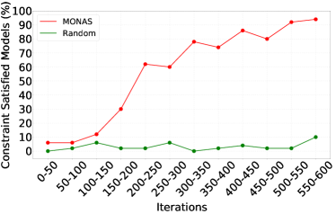
(a) Max Power 70W vs Random Search

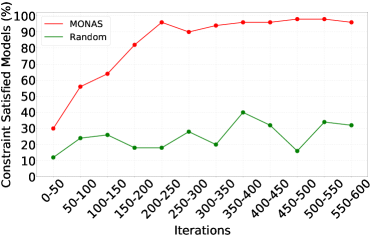
(b) Min Accuracy 0.85 vs Random Search

Figure 1: MONAS efficiently guides the search toward child networks satisfying constraints. X axis represents the number of iterations that robot network has been trained, and Y axis represent the percentage of child networks satisfying constraints. In the beginning MONAS has similar behaviors as random search; after 500 iterations, MONAS almost always generates child networks satisfying constraints.

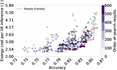
(a) $\alpha=0.25$ (focus on energy efficiency)

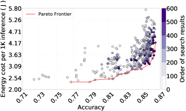
(b) $\alpha=0.75$ (focus on accuracy)

Figure 2: Effects of different $\alpha$ values. X axis represents the accuracy and Y axis is the energy consumption. Each sample here is a generated child network. Notice that (a) when alpha is 0.25, most of the generated child networks have lower energy consumption, and (b) when alpha is 0.75, most of the generated network have higher accuracies. Red curves indicate the Pareto frontier.

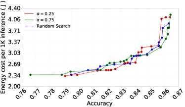
(a) Three Pareto frontiers achieved by: $\alpha=0.25$, $\alpha=0.75$, and random search

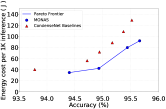
(b) Comparisons between MONAS and CondenseNet.

Figure 3: Pareto Frontiers achieved by different NAS algorithms and models. X axis is the accuracy and Y axis represents the energy consumption. (a) The Pareto frontier achieved by random search is in-between the ones achieved by $\alpha=0.25$ and $\alpha=0.75$, showing that MONAS is effective in searching for more energy-efficient or accurate models. (b) The Pareto frontier achieved by MONAS outperforms CondenseNet, showing MONAS is able to find a better model in terms of both accuracy and energy-efficiency.

Fig. 1 shows the reward functions proposed by MONAS efficiently guide NAS to focus on certain region of the search space for generating child networks that almost always satisfy constraints. Fig. 2 shows the effects of applying different $\alpha$ values to the reward function in Eq (1). With different $\alpha$ values, MONAS searches for different regions in the architectural space, leading to more energy-efficient networks in Fig. 2(a), or more accurate networks in Fig. 2(b). Fig. 3 provides the analyses of Pareto frontiers achieved by MONAS, random search, and CondenseNet. Experimental results confirm the effectiveness of MONAS. Specifically, in Fig. 3(b), the best model found by MONAS is compared with the best one selected from ³⁸. The Pareto Frontier in Fig. 3(b) demonstrates that the models found by MONAS have both higher accuracy and lower energy compared to the model designed by domain experts.

4 EA-like Multi-Objective NAS

In this section, we introduce an EA-like approach for multi-objective NAS: DPP-Net ². DPP-Net searches for neural networks with a predefined number of cells to achieve Pareto-optimal performance over multiple objectives. Each cell contains multiple layers, and each layer has the type “normalization (Norm)” or “convolutional (Conv).” DPP-Net progressively adds layers following the order: Norm-Conv-Norm-Conv (repeat). DPP-Net’s search space covers hand-crafted operations from MobileNet ³⁹, CondenseNet ³⁸, ShuffleNet ⁴⁰ to take advantages of experts’ knowledge on designing efficient CNNs. This improves the quality of each generated child network.

4.1 Search Algorithm

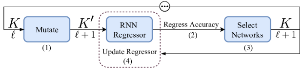
Figure 4: Diagram of the search algorithm in DPP-Net (from Dong et al. ⁴¹). The search process has four steps: (1) mutate to find child networks, (2) predict their accuracies, (3) select the networks achieving Pareto optimality to mutate for the next generation, and (4) update the regressor/predictor.

Inspired by ^{16, 42}, Dong et al. ⁴¹ adopt Sequential Model-Based Optimization (SMBO), an EA-like algorithm that contains four steps (see Fig. 4 for diagram):

1. Mutate. For each $\ell$-layers block, they enumerate all possible $\ell+1$-layers blocks. $K$ is the number of models to train, and ${K}^{\prime}$ is the number of models after mutation.

2. Regress accuracy. DPP-Net uses a Recurrent Neural Network (RNN) to predict a child network’s accuracy given its architecture with zero training.

3. Select networks. DPP-Net’s main contribution is to use Pareto Optimality over multiple objectives to select $K$ networks, shown in Fig. 4 step (3), rather than simply selecting the top $K$ accurate ones as in ¹⁶.

4. Update regressor. Each of the selected $K$ networks are trained for $N$ epochs. The child networks (as inputs) and their corresponding evaluation accuracies (as outputs) are used to update the RNN regressor.

4.2 Experimental Results

To begin with, Dong et al. ⁴¹ conduct the DPP-Net search with CIFAR-10 dataset with standard augmentation. After the search is done, the cell structure is used to form a larger model; then this model is trained and evaluated for ImageNet ⁴³ classification. All the experimental results in this section are excerpted from the original DPP-Net paper (Dong et al. ⁴¹).

Table.2 provides the details of the devices considered by DPP-Net during the search process. Mainly, there are three types of devices considered: workstation (WS), embedded system (ES) and mobile phones (M). When searching models for WS and ES, four objectives are considered: error rate, number of parameters, FLOPs, and actual inference time on the devices. When search models for mobile phones, memory usage is also included as the $5^{th}$ objective.

Table 2: Hardware Specifications of Devices in DPP-Net.

	Workstation (WS)	Embedded System (ES)	Mobile Phone (M)
Instance	Desktop PC	NVIDIA Jetson TX1	Xiaomi Redmi Note 4
CPU	Intel i5-7600	ARM Cortex57	ARM Cortex53
Cores	4	4	8
GHz	3.5	1.9	2.0
CUDA	Titan X (Pascal)	Maxwell 256	-
Memory	64 GB / 12 GB	4 GB	3 GB
Objectives	4	4	5

Table 3: Cifar10 classification results. Missing values are the metrics not reported by the original papers. The standard deviations reported in the bottom row for DPP-Net-Panacea are calculated across 10 runs. Numbers in bold font highlight the smallest value of each column.

	Device-agnostic metrics			Device-aware metrics
Model from previous works	Error rate	Params	FLOPs	Time-WS	Time-ES	Time-M	Mem-M
Real et al. 8	5.4	5.4M	-	-	-	-	-
NASNet-B 4	3.73	2.6M	-	-	-	-	-
PNASNet-1 16	4.01	1.6M	-	-	-	-	-
DenseNet-BC (k=12) 32	4.51	0.80M	-	-	-	0.273	79MB
CondenseNet-86 38	5.0	0.52M	65.8M	0.009	0.090	0.149	113MB
	Device-agnostic metrics			Device-aware metrics
Model from DPP-Net	Error rate	Params	FLOPs	Time-WS	Time-ES	Time-M	Mem-M
DPP-Net-PNAS	4.36	11.39M	1364M	0.013	0.062	0.912	213MB
DPP-Net-WS	4.78	1.00M	137M	0.006	0.075	0.210	129MB
DPP-Net-ES	4.93	2.04M	270M	0.007	0.044	0.381	100MB
DPP-Net-M	5.84	0.45M	59.27M	0.008	0.065	0.145	58MB
DPP-Net-Panacea	4.62 $\pm$ 0.23	0.52M	63.5M	0.009 $\pm$ 7.4e-5	0.082 $\pm$ 0.011	0.149 $\pm$ 0.017	104MB

Results on CIFAR-10. Table 3 provides the performance comparisons among DPP-Net, previous NAS literatures ^{4, 8, 16} and the state-of-the-art handcrafted mobile CNN models: DenseNet-BC and CondenseNet ^{38, 32}. Among all networks, DPP-Net-Panacea (bottom row) has a small error rate and performs relatively well on every objective. We also include the results of the neural network found by DPP-Net with PNAS ¹⁶ criterion: using classification accuracy as the only objective. DPP-Net-PNAS has a large number of parameters and the corresponding inference time is slow; yet, it achieves a smaller error rate. This shows DPP-Net provides a flexible and effective framework to search for device-aware, high-performance neural networks.

Table 4: ImageNet classification results. Time-ES represents the inference time on the embedded system; Time-M and Mem-M are the inference time and memory usage, respectively, when the model is deployed on a mobile phone.

Model	Top-1	Top-5	Params	FLOPs	Time-ES	Time-M	Mem-M
Densenet-121 32	25.02	7.71	-	-	0.084	1.611	466MB
Densenet-169 32	23.80	6.85	-	-	0.142	1.944	489MB
Densenet-201 32	22.58	6.34	-	-	0.168	2.435	528MB
ShuffleNet 1x (g=8) 40	32.4	-	5.4M	140M	0.051	0.458	243MB
MobileNetV2 44	28.3	-	1.6M	-	0.032	0.777	270MB
Condensenet-74 (G=4)38	26.2	8.30	4.8M	529M	0.072	0.694	238MB
NASNet (Mobile) 4	26.0	8.4	5.3M	564M	0.244	-	-
DPP-Net-PNAS	24.16	7.13	77.16M	9276M	0.218	5.421	708MB
DPP-Net-Panacea	25.98	8.21	4.8M	523M	0.069	0.676	238MB

Results on ImageNet. Table 4 provides the comparisons among DPP-Net and other models on the ImageNet classification task. Notice that DPP-Net-Panacea outperforms the state-of-the-art, hand-crafted architecture Condensenet-74 in almost every aspect. Moreover, DPP-Net-Panacea also outperforms NASNet (Mobile), a single-objective, state-of-the-art NAS approach ⁴ in every objective. These results demonstrate that high model accuracy and device-related objectives (e.g., latency) can be achieved/optimized at the same time, without compromising one over the others.

5 Discussions

In this paper, we survey recent literatures on NAS and summarize them into four categories: (a) RL, (b) EA, (c) search acceleration and (d) multi-objective. Also, currently there are two main streams of designing the search space for NAS: covering the entire network (macro) or only one cell (micro).

We also deep dive into two recent advancements of multi-objective NAS: MONAS and DPP-Net. MONAS adapts rewards to application-specific constraints and effectively guide the search process to find the models of interest, such as achieving higher accuracy and at the same time lower energy consumption.

To the best of our knowledge, DPP-Net is the first device-aware NAS outperforming state-of-the-art handcrafted mobile CNNs. Experimental results on CIFAR-10 demonstrate the effectiveness of Pareto-optimal networks found by DPP-Net, for three different devices: (a) a workstation with NVIDIA Titan X GPU, (b) NVIDIA Jetson TX1 embedded system, and (c) mobile phone with ARM Cortex-A53. Compared to CondenseNet and NASNet (Mobile), DPP-Net achieves better performances: higher accuracy & shorter inference time on these various devices.

Most of the successes achieved by NAS (both single and multiple objectives) are in convolutional neural networks and image-related domains. Therefore, we believe exploring NAS into other domains is a straight-line and important future work. Furthermore, all previous works on multi-objective NAS adapt existed search space and acceleration methods. In other words, no search space or acceleration methods are proposed specifically for multi-objective NAS. Given the importance and high complexity of multi-objective NAS, we believe designing search space or acceleration method will be a critical and challenging future direction in this field.

References

- [1] Chi-Hung Hsu, Shu-Huan Chang, Da-Cheng Juan, Jia-Yu Pan, Yu-Ting Chen, Wei Wei, and Shih-Chieh Chang. Monas: Multi-objective neural architecture search using reinforcement learning. arXiv preprint arXiv:1806.10332, 2018.
- [2] Jin-Dong Dong, An-Chieh Cheng, Da-Cheng Juan, Wei Wei, and Min Sun. Dpp-net: Device-aware progressive search for pareto-optimal neural architectures. arXiv preprint arXiv:1806.08198, 2018.
- [3] Barret Zoph and Quoc V Le. Neural architecture search with reinforcement learning. ICLR’17, 2016.
- [4] Barret Zoph, Vijay Vasudevan, Jonathon Shlens, and Quoc V Le. Learning transferable architectures for scalable image recognition. arXiv preprint arXiv:1707.07012, 2017.
- [5] Hanxiao Liu, Karen Simonyan, Oriol Vinyals, Chrisantha Fernando, and Koray Kavukcuoglu. Hierarchical representations for efficient architecture search. ICLR’18, 2017.
- [6] Bowen Baker, Otkrist Gupta, Nikhil Naik, and Ramesh Raskar. Designing neural network architectures using reinforcement learning. ICLR’17, 2016.
- [7] Lingxi Xie and Alan Yuille. Genetic cnn. ICCV’17, 2017.
- [8] Esteban Real, Sherry Moore, Andrew Selle, Saurabh Saxena, Yutaka Leon Suematsu, Quoc Le, and Alex Kurakin. Large-scale evolution of image classifiers. ICML’17, 2017.
- [9] Esteban Real, Alok Aggarwal, Yanping Huang, and Quoc V Le. Regularized evolution for image classifier architecture search. arXiv preprint arXiv:1802.01548, 2018.
- [10] Andrew Brock, Theodore Lim, James M Ritchie, and Nick Weston. Smash: one-shot model architecture search through hypernetworks. ICLR’18, 2017.
- [11] Han Cai, Tianyao Chen, Weinan Zhang, Yong Yu, and Jun Wang. Efficient architecture search by network transformation. AAAI’18, 2017.
- [12] Han Cai, Jiacheng Yang, Weinan Zhang, Song Han, and Yong Yu. Path-level network transformation for efficient architecture search. arXiv preprint arXiv:1806.02639, 2018.
- [13] Zhao Zhong, Junjie Yan, and Cheng-Lin Liu. Practical network blocks design with q-learning. AAAI’18, 2017.
- [14] Hieu Pham, Melody Y Guan, Barret Zoph, Quoc V Le, and Jeff Dean. Efficient neural architecture search via parameter sharing. arXiv preprint arXiv:1802.03268, 2018.
- [15] Thomas Elsken, Jan-Hendrik Metzen, and Frank Hutter. Simple and efficient architecture search for convolutional neural networks. arXiv preprint arXiv:1711.04528, 2017.
- [16] Chenxi Liu, Barret Zoph, Jonathon Shlens, Wei Hua, Li-Jia Li, Li Fei-Fei, Alan Yuille, Jonathan Huang, and Kevin Murphy. Progressive neural architecture search. arXiv preprint arXiv:1712.00559, 2017.
- [17] Gabriel Bender, Pieter-Jan Kindermans, Barret Zoph, Vijay Vasudevan, and Quoc Le. Understanding and simplifying one-shot architecture search. In International Conference on Machine Learning, pages 549–558, 2018.
- [18] Hanxiao Liu, Karen Simonyan, and Yiming Yang. Darts: Differentiable architecture search. arXiv preprint arXiv:1806.09055, 2018.
- [19] Thomas Elsken, Jan Hendrik Metzen, and Frank Hutter. Multi-objective architecture search for cnns. arXiv preprint arXiv:1804.09081, 2018.
- [20] Sean C Smithson, Guang Yang, Warren J Gross, and Brett H Meyer. Neural networks designing neural networks: multi-objective hyper-parameter optimization. In Proceedings of the 35th International Conference on Computer-Aided Design, page 104. ACM, 2016.
- [21] Ye-Hoon Kim, Bhargava Reddy, Sojung Yun, and Chanwon Seo. Nemo: Neuro-evolution with multiobjective optimization of deep neural network for speed and accuracy. ICML’17 AutoML Workshop, 2017.
- [22] Yanqi Zhou, Siavash Ebrahimi, Sercan Ö Arık, Haonan Yu, Hairong Liu, and Greg Diamos. Resource-efficient neural architect. arXiv preprint arXiv:1806.07912, 2018.
- [23] Mingxing Tan, Bo Chen, Ruoming Pang, Vijay Vasudevan, and Quoc V Le. Mnasnet: Platform-aware neural architecture search for mobile. arXiv preprint arXiv:1807.11626, 2018.
- [24] Alex Krizhevsky, Ilya Sutskever, and Geoffrey E Hinton. Imagenet classification with deep convolutional neural networks. In Advances in neural information processing systems, pages 1097–1105, 2012.
- [25] Awni Hannun, Carl Case, Jared Casper, Bryan Catanzaro, Greg Diamos, Erich Elsen, Ryan Prenger, Sanjeev Satheesh, Shubho Sengupta, Adam Coates, et al. Deep speech: Scaling up end-to-end speech recognition. arXiv preprint arXiv:1412.5567, 2014.
- [26] Ilya Sutskever, Oriol Vinyals, and Quoc V Le. Sequence to sequence learning with neural networks. In Advances in neural information processing systems, pages 3104–3112, 2014.
- [27] Renato Negrinho and Geoff Gordon. Deeparchitect: Automatically designing and training deep architectures. arXiv preprint arXiv:1704.08792, 2017.
- [28] Thomas Elsken, Jan Hendrik Metzen, and Frank Hutter. Neural architecture search: A survey. arXiv preprint arXiv:1808.05377, 2018.
- [29] Shreyas Saxena and Jakob Verbeek. Convolutional neural fabrics. In Advances in Neural Information Processing Systems, pages 4053–4061, 2016.
- [30] Hector Mendoza, Aaron Klein, Matthias Feurer, Jost Tobias Springenberg, and Frank Hutter. Towards automatically-tuned neural networks. In Workshop on Automatic Machine Learning, pages 58–65, 2016.
- [31] Kaiming He, Xiangyu Zhang, Shaoqing Ren, and Jian Sun. Deep residual learning for image recognition. In Proceedings of the IEEE conference on computer vision and pattern recognition, pages 770–778, 2016.
- [32] Gao Huang, Zhuang Liu, Kilian Q Weinberger, and Laurens van der Maaten. Densely connected convolutional networks. CVPR’17, 2017.
- [33] David E Goldberg and Kalyanmoy Deb. A comparative analysis of selection schemes used in genetic algorithms. In Foundations of genetic algorithms, volume 1, pages 69–93. Elsevier, 1991.
- [34] Yukang Chen, Qian Zhang, Chang Huang, Lisen Mu, Gaofeng Meng, and Xinggang Wang. Reinforced evolutionary neural architecture search. arXiv preprint arXiv:1808.00193, 2018.
- [35] Tobias Domhan, Jost Tobias Springenberg, and Frank Hutter. Speeding up automatic hyperparameter optimization of deep neural networks by extrapolation of learning curves. In IJCAI, volume 15, pages 3460–8, 2015.
- [36] Bowen Baker, Otkrist Gupta, Ramesh Raskar, and Nikhil Naik. Accelerating neural architecture search using performance prediction. 2018.
- [37] Haifeng Jin, Qingquan Song, and Xia Hu. Efficient neural architecture search with network morphism. arXiv preprint arXiv:1806.10282, 2018.
- [38] Gao Huang, Shichen Liu, Laurens van der Maaten, and Kilian Q Weinberger. Condensenet: An efficient densenet using learned group convolutions. arXiv preprint arXiv:1711.09224, 2017.
- [39] Andrew G Howard, Menglong Zhu, Bo Chen, Dmitry Kalenichenko, Weijun Wang, Tobias Weyand, Marco Andreetto, and Hartwig Adam. Mobilenets: Efficient convolutional neural networks for mobile vision applications. arXiv preprint arXiv:1704.04861, 2017.
- [40] Xiangyu Zhang, Xinyu Zhou, Mengxiao Lin, and Jian Sun. Shufflenet: An extremely efficient convolutional neural network for mobile devices. arXiv preprint arXiv:1707.01083, 2017.
- [41] Jin-Dong Dong, An-Chieh Cheng, Da-Cheng Juan, Wei Wei, and Min Sun. Ppp-net: Platform-aware progressive search for pareto-optimal neural architectures. 2018.
- [42] Frank Hutter, Holger H Hoos, and Kevin Leyton-Brown. Sequential model-based optimization for general algorithm configuration. International Conference on Learning and Intelligent Optimization, 2011.
- [43] Jia Deng, Wei Dong, Richard Socher, Li-Jia Li, Kai Li, and Li Fei-Fei. Imagenet: A large-scale hierarchical image database. In Computer Vision and Pattern Recognition, 2009. CVPR 2009. IEEE Conference on, pages 248–255. IEEE, 2009.
- [44] Mark Sandler, Andrew Howard, Menglong Zhu, Andrey Zhmoginov, and Liang-Chieh Chen. Inverted residuals and linear bottlenecks: Mobile networks for classification, detection and segmentation. arXiv preprint arXiv:1801.04381, 2018.