MARL-FWC: Optimal Coordination of Freeway Traffic Control Measures

Abstract

The objective of this article is to optimize the overall traffic flow on freeways using multiple ramp metering controls plus its complementary Dynamic Speed Limits (DSLs). An optimal freeway operation can be reached when minimizing the difference between the freeway density and the critical ratio for maximum traffic flow. In this article, a Multi-Agent Reinforcement Learning for Freeways Control (MARL-FWC) system for ramps metering and DSLs is proposed. MARL-FWC introduces a new microscopic framework at the network level based on collaborative Markov Decision Process modeling (Markov game) and an associated cooperative Q-learning algorithm. The technique incorporates payoff propagation (Max-Plus algorithm) under the coordination graphs framework, particularly suited for optimal control purposes. MARL-FWC provides three control designs: fully independent, fully distributed, and centralized; suited for different network architectures. MARL-FWC was extensively tested in order to assess the proposed model of the joint payoff, as well as the global payoff. Experiments are conducted with heavy traffic flow under the renowned VISSIM traffic simulator to evaluate MARL-FWC. The experimental results show a significant decrease in the total travel time and an increase in the average speed (when compared with the base case) while maintaining an optimal traffic flow.

Keywords Multi-agent system  $\cdot$ Intelligent transportation system  $\cdot$ Adaptive traffic control  $\cdot$ Freeway  $\cdot$ Ramp metering  $\cdot$ Max-plus  $\cdot$ Q-learning  $\cdot$ Sequential decision problem

1 Introduction

The world is experiencing a period of rapid urbanization, with more than 60 percent of the world population expected to live in cities by 2025 Prendinger et al. (2013). The huge increase in the number and length of traffic jams on freeways has led to the use of several dynamic traffic management measures. The sophistication of traffic network demands, as well as their severity, have also increased recently. Consequently, the need for an optimal and reliable traffic control, for urban freeways networks, has become more and more critical.

Generally, there are three freeway control strategies: on-ramp control, mainline control, and DSLs control. Two signals are only generated by a ramp metering device: red and green (no yellow), controlled by a smart or basic controller that regulates the flow of traffic entering the freeway according to the current traffic volume. We aim to control the number of vehicles entering the mainstream freeway from the ramp merging area. This optimizes the freeway density below the critical one. In order to achieve this flow, optimal coordination of the freeway traffic control measures over the network level is highly needed.

Machine Learning (ML) is one of the fastest growing areas of science. It has been been used in many applications; e.g., traffic signal control Khamis and Gomaa (2014, 2012); Khamis et al. (2012b, a), car-following models Zaky et al. (2015), bioinformatics Khamis et al. (2015); Khamis and Gomaa (2015), etc. Reinforcement Learning (RL) is a machine learning technique that addresses the inquiry of how an autonomous agent can learn behavior through trial and error interaction with the dynamic environment to accomplish its goals Kaelbling and Moore (1996). In order to solve the problem of optimal metering rate on the network level; a collaborative Multi-Agent System (MAS) Vlassis et al. (2004) based on reinforcement learning is appropriate. A collaborative MAS is defined as the system in which the agents are designed to act together in order to optimize the sequence of actions. The framework of the Coordination Graphs (CGs) Guestrin et al. (2001) is utilized which is designed based on the dependencies between agents. It decomposes the global payoff function into a sum of local payoffs based on that dependency.

Traffic congestion is a challenging problem faced in everyday life. It has multiple negative effects on the average speed, overall total travel time, fuel consumption, safety (primary cause of accidents), and environment (air pollution). Hence, comes the need for an intelligent reliable traffic control system. The objective of this article is to optimize the overall traffic congestion in freeways via multiple ramps metering controls plus its complementary multiple DSLs controls. Maximize the freeway traffic flow by always keeping the freeway density within a small margin of the critical ratio (which is calculated using the calibrating fundamental diagram of the traffic flow). Preventing the breakdown of a downstream bottleneck through the regulation of traffic stream speed. Preventing the capacity drop at the merging area via ramp metering control plus its complementary DSLs control, i.e., complements the function of RM when the flow is above the critical ratio.

In this article, a Multi-Agent Reinforcement Learning for Freeways Control (MARL-FWC) system for ramp metering and dynamic speed limit is proposed based on a Reinforcement Learning density Control Agent (RLCA). MARL-FWC introduces a new microscopic framework at the network level based on collaborative Markov Decision Process (Markov game) modeling and an associated cooperative Q-learning algorithm. The technique incorporates payoff propagation (Max-Plus algorithm) under the coordination graphs framework, particularly suited for optimal control purposes. A model for the local payoff, the joint payoff, as well as the global payoff is proposed. MARL-FWC provides three control designs: fully independent, fully distributed, and centralized; suited for different network architectures.

Preliminary results of this work have been published in Fares and Gomaa (2014, 2015). In this article, a more detailed description and improvements on MARL-FWC are provided. An adaptive objective function plus DSLs are presented. The new approach for ramp metering plus DSLs have shown considerable improvement over the base case. In addition, a detailed survey of the state-of-the-art work is presented.

The article is organized as follows. Section 2 briefly illustrates the related work. Section 3 describes the RL approach, particularly the Q-learning algorithm. In addition, it briefly describes the Max-Plus algorithm and associated CGs framework. Section 4 illustrates the design of the RLCA. Furthermore, it demonstrates the design of three approaches to solve the freeway congestion problem, particularly the design of the global and joint payoff. And finally it depicts the MARL-FWC for adaptive ramp metering plus DSLs. The VISSIM traffic simulator capabilities are also presented. Section 5 represents the results of applying MARL-FWC to different traffic networks and compares its performance to the base case. Finally, Section 6 summarizes the conclusions.

2 Related Work

Ramp metering and speed limits lay under the advanced traffic management systems and are considered one of the most effective traffic control strategies on the freeways recently. Intelligent ramp metering and DSLs mainly depend on the current traffic state. This gives them advance over the fixed time (predefined time signal) and actuated one (sensor located underground to detect the vehicles and change the signal to green). Several different techniques have been recently applied including: Intelligent control theory, fuzzy control Yu et al. (2012); Ghods et al. (2009), neural network control Liang et al. (2010); Li and Liang (2009), and even some hybrid of them  Feng et al. (2011).

In this article, a new framework of ramp metering in the network level is proposed based on modeling by collaborative Markov Decision Process (Markov Game) Vlassis et al. (2004); Guestrin (2003) and an associated cooperative Q-learning algorithm, which is based on a payoff propagation algorithm Pearl (1988) under the CGs framework. MARL-FWC avoids not only the locality of all techniques mentioned above, but also the computational complexity and the risk of being trapped in local optimum of the Model Predictive Control (MPC) Ernst et al. (2009). In addition, the solid knowledge of the system considered to extract the rules as in the fuzzy control system. MARL-FWC has been extensively tested in order to assess the proposed model of the joint payoff, as well as the global payoff.

3 Single and Multi-Agent Algorithms

In this section, RL approach is illustrated. This section describes the Q-learning algorithm and shows the difference between the traditional Q-learning and the modified one (temporal difference algorithm). Then, this section describes briefly the Max-Plus algorithm. This algorithm is used to determine the option joint action in connected graph, so the coordination graphs framework is introduced. Finally, freeway traffic flow model is illustrated in details, particularly the fundamental diagram of the traffic flow.

3.1 Reinforcement learning

The RLCA is interacting with the traffic network. The agent receives the traffic state from the network detectors. This state consists of the number of vehicles $N_{t}$ and the current density $\rho_{t}$. Based on this information the RLCA chooses an action $a_{t}$. As a consequence of $a_{t}$; the agent receives a reward $r_{t}$ that keeps the density of the network around a small neighborhood of the critical density. The aim of the agent is to learn a policy which maps an arbitrary state into an optimal action $\pi:S\longrightarrow A$. An optimal action is an action that optimizes the long-term cumulative discounted reward, thus the optimization is done over an infinite horizon. Given a policy $\pi$, the value function corresponding to $\pi$ is stated by Eq. 1:

$$V^{\pi}(s_{t})=r_{t}+\gamma^{1}r_{t+1}+\gamma^{2}r_{t+2}+....=\sum_{i=1}^{\infty}\gamma^{i}r_{t+i}$$ (1)

where $\gamma\in(0,1)$ is the discount factor and is necessary for the convergence of the previous formula. A policy $\pi^{*}$ is optimal if its corresponding value function is optimal as in Eq. 2, that is, for any control policy $\pi$ and any state $s$ (here it is assumed that the objective function is to be maximized):

$$V^{{\pi}^{\ast}}(s)\geq V^{\pi}(s)$$ (2)

3.2 Q-Learning

A Q-learning agent could learn based on experienced action sequence actuated in a Markovian environment. In fact, Q-learning is a kind of MDP. In his proof of convergence, Watkins Watkins and Dayan (1992) assumed a lookup table to represent the value function Watkins and Dayan (1992).

This algorithm is guaranteed to converge to the optimal $Q$-values with a probability of one under some conditions: the $Q$-function is represented exactly using a lookup table and each state-action pair is visited infinitely often. After convergence to the optimal $Q$-function $Q^{*}$, the optimal control policy can be extracted as in Eq. 3:

$$\pi^{*}(s)=\operatorname*{arg\,max}_{a\in A}Q^{*}(s,a)$$ (3)

And the optimal value function (the function that gives a valuation of the states; it can be viewed as a projection of the $Q$-function over the action space) is represented as in Eq. 4:

$$V^{*}(s)=V^{{\pi}^{\ast}}(s)=\max_{a}Q^{*}(s,a)$$ (4)

3.2.1 A modified Q-learning: Temporal difference algorithm

As long as there is no model of the environment (unknown environment), so the infinite sum of the discount reward is no longer considered as a function of state $s$ only as in Dynamic Programming (DP) value iteration Bertsekas (1996), but as a function of the state action pair $(s,a)$. That is why such a $Q$-function Watkins and Dayan (1992) is used. When the agent is in state $s$ and the agent performs action $a$ and its long-term reward is $Q(s,a)$; if each state and action pairs are visited infinitely often; then $Q(s,a)$ converges to $Q^{*}(s,a)$ Kaelbling and Moore (1996). Based on such long-term reward the optimal policy is calculated using Eq. (3). $Q$-learning converges no matter how the actions during the learning are chosen, as long as every action is selected infinitely often (fair action selection strategy). A modification of the traditional $Q$-learning rule is in Eq. (3.2.1). This new scheme is called a Temporal Difference (TD) learning where $\alpha$ is the learning rate Kaelbling and Moore (1996).

$$Q^{new}_{t}(s,a)=Q^{old}_{t-1}(s,a)+$$

$$\underbrace{\alpha_{t}(s,a)}_{\text{{learning rate}}}\left[\overbrace{\underbrace{R_{t}(s,a)}_{\text{reward}}+\underbrace{\gamma}_{\text{dis. fac.}}\>\max_{a^{{}^{\prime}}}Q_{t-1}^{old}(s^{{}^{\prime}},a^{{}^{\prime}})-Q_{t-1}^{old}(s,a)}^{\text{TD-Error}}\right]$$ (5)

For alpha value, the easiest approach is to take a fixed value $\alpha$, but even better to use a variable $\alpha$. Eq. (6) is one possibility where $b(s,a)$ is the number of times the action $a$ has been chosen in the state $s$.

$$\alpha_{t}(s,a)=\frac{1}{1+b_{t}(s,a)}$$ (6)

There are two extreme possibilities for the best action selection strategy Kaelbling and Moore (1996). One extreme is to always choose the action randomly. This what is called exploration; just explore what the environment gives in terms of feedback. In the beginning of the learning process this is a good idea. But after some time when the RLCA has already learned, other alternative can be tried which is to select the best action. This is called exploitation. In the present case, a combination of exploitation and exploration are used by using $\varepsilon$-greedy action selection strategy, that is with a certain probability $\varepsilon$; the agent always selects a random action. The state space, the action space and the reward function of the single control agent are described in Fares and Gomaa (2014) and Subsection 4.1. The joint action space and the (joint and global) payoff function of collaborative multi-agent are described in detail in Fares and Gomaa (2015) and Subsection 4.2.

3.3 Payoff propagation

In this subsection, the problem of dynamics in MASs is discussed and the suggestion that the agents should take the behavior of other agents into account.

3.3.1 Coordination graphs

CGs Guestrin et al. (2001) can be demonstrated as an undirected graph $G=(V,\;E)$, where each node $i\in V$ represents an agent, and an edge $e(i,\;j)\in E$ between agents $i,\;j$ means that a dependency exists between them ($j\in\mathrm{\Gamma}(i)$ and $i\in\mathrm{\Gamma}(j)$). Thus, they need to coordinate their actions. CGs allow for the decomposition of a coordination problem into several smaller sub-problems that are easier to solve. CGs have been represented in the context of probabilistic graphs, where the global function, consisting of many variables, is decomposed into local functions. Each of these local functions depends only on a subset of the variables. The Maximum A Posteriori (MAP) configuration (see Subsection 3.3.2) is then estimated by sending locally optimized messages between connected agents (nodes) in the CGs. Even though the message-passing algorithm is developed for estimating the MAP configuration in a probabilistic graph, it is applicable for estimating the optimal joint action of a group of agents in CGs. Because in both situations, the function that is being optimized is decomposed in local terms Kok and Vlassis (2006).

In collaborative multi-agent systems, the CGs framework Papageorgiou et al. (1991) assumes the action of an agent $i$ only depends on a subset of other agents ($j\in\mathrm{\Gamma}(i)$) which may influence its state. The global payoff function $u(\mathbf{a})$ is then broken down into a linear combination of local payoff functions $f_{i}(\mathbf{a_{i}})$. The proposed design of the local and global payoff is found in Subsections 4.2.1 and 4.2.2 respectively. The global $Q$-function $Q(\mathbf{s},\;\mathbf{a})$ is then decomposed into a sum of local functions given by:

$$Q(\mathbf{s},\;\mathbf{a})=\sum_{i=1}^{n}Q_{i}({s_{i}},\;\mathbf{a_{i}})$$ (7)

Where: $\mathbf{a}=(a_{1},...,a_{n})$ is the joint action resulting from: each agent $i$ selects an action $a_{i}$ from its action set $A_{i}$, $\mathbf{s}=(s_{1},...,s_{n})\in S_{1}\times\cdots\times S_{n}$ is the joint state. The joint $Q$-function $Q_{i}({s_{i}},\mathbf{a_{i}})$ depends only on $\mathbf{a_{i}}\subseteq\mathbf{a}$, where $\mathbf{a_{i}}\in A_{i}\times\prod_{j\in\mathrm{\Gamma(i)}}A_{j}$, $\mathrm{\Gamma(i)}$ is the set of neighborhoods of agent $i$. The decomposition in Eq. (7) can be demonstrated in Fig. 1(a) (an example of a CGs of four agents where the dependence among agents is decomposed into pair-wise functions Yedidia et al. (2003)); where $f_{ij}$ is the joint payoff between agent $i$ and agent $j$.

3.3.2 Max-Plus algorithm

The Max-Plus algorithm approximates the optimal joint action by iteratively sending locally optimized messages between connected agents (neighbors) in the coordination graph. It is similar to the belief propagation or the max-product algorithm, which estimates the MAP configuration in Belief Networks Kschischang et al. (2001). Max-Plus was originally developed for computing MAP solutions in Bayesian networks Pearl (1988). The MAP for each agent is estimated using only the incoming messages from other agents. It has been shown that the message updates converge to a fixed point after a finite number of iterations for cycle free graphs. The message mainly depends on the decomposition given by Eq. (7) and can be defined as follows:

$$\mu_{ij}(a_{j})=\max_{a_{i}}\left\{f_{i}\left(a_{i}\right)+f_{ij}(a_{i},a_{j})+\sum_{k\in\mathrm{\Gamma(i)}\backslash j}\mu_{ki}(a_{i})\right\}$$ (8)

Where: $k\in\mathrm{\Gamma(i)}\backslash j$ is the subset of all neighbors connected to $i$ except $j$, and $\mu_{ij}(a_{j})$ is the message from an agent $i$ to agent $j$ after agent $j$ preforms the action $a_{j}$ as an evaluation of the influence of this action on agent $i$ state. The message approximates the maximum reward agent $i$ can achieve for a committed action of agent $j$. This message is the max-sum of the local payoff $f_{i}\left(a_{i}\right)$, the joint payoff $f_{ij}(a_{i},a_{j})$ and all incoming messages agent $i$ received except that from agent $j$. The design of the joint payoff is found in detail in Subsection 4.2.2. Figure 1(b) shows a CG with three agents and the corresponding messages.

If the graph has no cycle, Max-Plus always converges after a finite number of steps to a fixed point in which the messages are changed below a certain threshold Wainwright et al. (2004). At each time step, the value for an action $a_{i}$ of an agent $i$ can be determined as follows:

$$g_{i}(a_{i})=f_{i}(a_{i})+\sum_{j\in\Gamma(i)}\mu_{ji}(a_{i})$$ (9)

When the convergence is held, optimal joint action $\mathbf{a}$ has the element $a^{\ast}_{i}$ which can be computed as follows:

$$a^{\ast}_{i}=\operatorname*{arg\,max}_{a_{i}}g_{i}(a_{i})$$ (10)

In the Max-Plus algorithm; at each iteration, an agent $i$ sends a message $\mu_{ij}(a_{j})$ to each neighbor $j\in\mathrm{\Gamma(i)}$ given the joint payoff $f_{ij}$ and current incoming messages it has received and also computes its current optimal action given all the messages it has received so far that is why it is called anytime algorithm Kok and Vlassis (2006). The process continues until all messages converge, or a deadline signal is received which means the agents must report their individual actions. In the anytime algorithm, the joint action Eq. 10 is only updated when the corresponding global payoff improves.

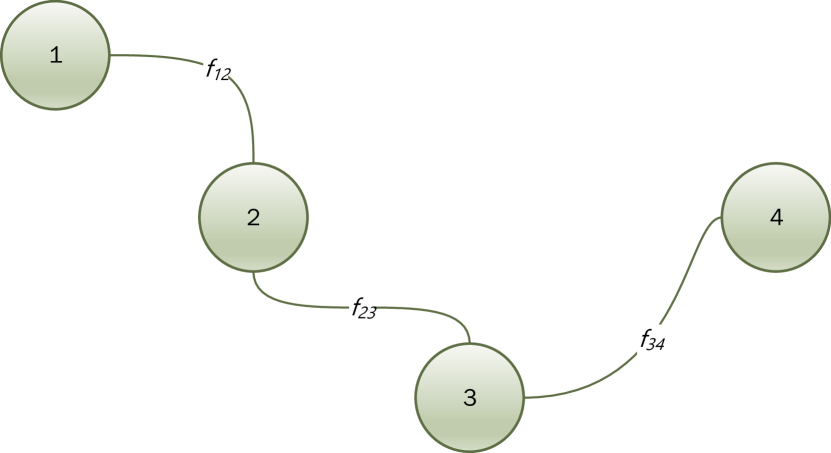
(a) CG involving 4 agents with only pair-wise dependencies.

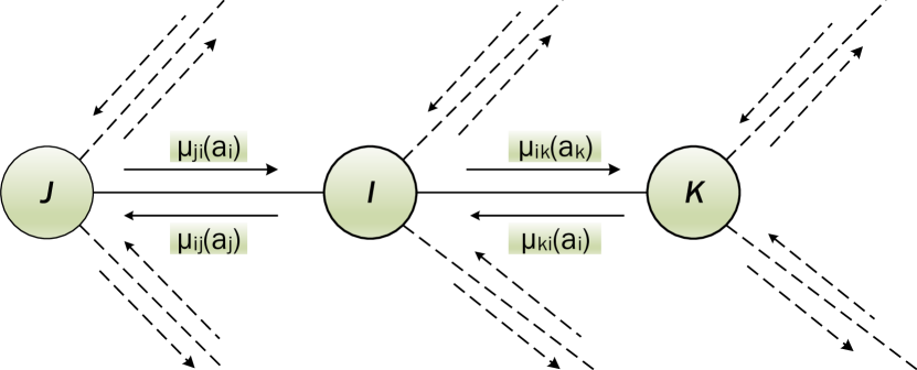
(b) Representation of the different $\mu_{ij}$ sent between neighboring agents.

Figure 1: Payoff propagation: Coordination graphs and Max plus.

4 MARL-FWC Architecture

Figure 2 demonstrates MARL-FWC architecture. MARL-FWC consists of two layers; the intelligent control layer and the configuration layer. The configuration layer consists of three blocks:

• Ramp metering parameters: configure the ramp metering.

• DSLs parameters: configure the DSLs.

• Agents’ parameters: configure the control agent.

The main task of the configuration layer is to configure the control layer. The control layer consists of three interacting modules (blocks):

• Environment module (VISSIM simulator): models the traffic network.

• Multi-agent reinforcement-learning module (Computing environment): implements different controls strategies.

• Interface module (VISSIM interface): facilitates the interaction between the Multi-agent reinforcement-learning module and the environment module.

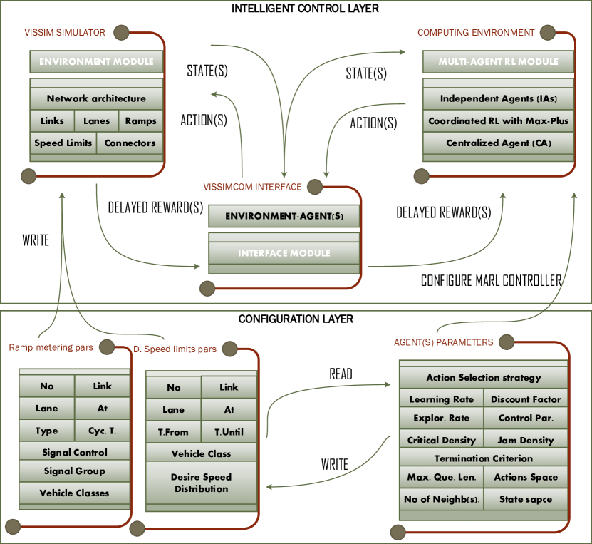
Figure 2: MARL-FWC architecture.

In the following subsections, the main components of the MARL-FWC architecture are described in details, e.g., RLCA (used in the IAs framework).

4.1 MARL-FWC with single ramp and RLCA as control measure

In the following subsections, all the components of the Markov decision process that corresponds to the on-ramp metering RLCA are described.

4.1.1 State space

The state space is three-dimensional where each state vector $s_{t+1}$ at time $t+1$ consists of the following components: the number of vehicles in the freeway $N(t+1)$ (see Fares and Gomaa (2014)), the number of vehicles that entered the freeway from ramp $\Delta N(t+1)$, and the ramp traffic signal at the previous time step $Ts(t)$.

4.1.2 Action space

By metering on the on-ramp, the red and green phases of the ramp metering change in order to control the flow entering the freeway from the merging point. So, the action space is modeled as consisting only of two actions: red and green. The optimal action is then chosen based on Eq. (3).

4.1.3 Reward function

Since the RLCA’s goal is to keep the freeway density $\rho$ around a small neighborhood of the critical density $\rho_{cr}$, the reward function is designed so as to depend on the current freeway density $\rho$ and how much it deviates from the critical density $\rho_{cr}$. Hence, the reward of taking an action $a$ in state $s$ is designed as following:

$$Minimize\;\;O=|\rho-\rho_{cr}|:r(s,a)=-|\rho-\rho_{cr}|$$ (11)

As long as the $Q$-value Eq. (3.2.1) (as a function of current state and action) is maximized, the difference between the freeway density $\rho$ and the critical density $\rho_{cr}$ is minimized. Therefore, the best utilization of the freeway is achieved without causing congestion.

4.2 MARL-FWC based on multi-agent and cooperative Q-learning

4.2.1 Independent agents

The “independent learning” is the first proposed design to solve the freeway congestion problem (Fig. 3(a)). The $Q$-function is updated as follows:

$$Q_{i}^{new}(s_{i},a_{i})=Q_{i}^{old}(s_{i},a_{i})+$$

$$\alpha\left[R(s_{i},a_{i})+\gamma\;\max_{a^{\prime}_{i}}Q_{i}^{old}(s^{\prime}_{i},a^{\prime}_{i})-Q_{i}^{old}(s_{i},a_{i})\right]$$ (12)

Where: $R(s_{i},a_{i})=-{|\rho(s_{i},a_{i})-\rho_{cr}|}$ from Eq. (11), with such conception of the objective function, the agents try to keep the freeway density within a small margin of the critical ratio; that ensures the maximum utilization of the freeway without entering in congestion. In this $Q$-function design, the agents are partially observing the environment. An agent observes its state which is defined as the number of vehicles in the areas of interest associated with that agent and chooses the local action either red or green, independent of all other agent actions. This cheap design is recommended when the distances between ramps are too long.

4.2.2 Coordinated reinforcement learning with Max-plus

The second design is considered as a completely distributed design (Fig. 3(b)). It considers a MARL based design. This design works on the network level and is based on modeling by collaborative Markov Decision Process (Markov Game) and an associated cooperative Q-learning algorithm. This design incorporates a payoff propagation (Max-plus algorithm) under the coordination graphs framework, particularly suited for optimal control purposes. In this design, the control agent coordinates its actions with its neighboring agents (message passing algorithm). The agent updates the cooperative $Q$-function globally as follows:

$$Q_{i}^{new}(s_{i},\mathbf{a_{i}})=Q_{i}^{old}(s_{i},\mathbf{a_{i}})+$$

$$\alpha\left[R(\textbf{s},\textbf{a})+\gamma\;\max_{\mathbf{a^{\prime}}}Q^{old}(\mathbf{s^{\prime}},\mathbf{a^{\prime}})-Q^{old}(\mathbf{s},\mathbf{a})\right]$$ (13)

Where:

• $Q(\mathbf{s},\mathbf{a})$ can be computed using Eq. (7).

• $\alpha$ can be computed using Eq. (6).

• R(s,a) can be figured out by the proposed conception of the global reward function using the harmonic mean. With such design, it is guaranteed the balance between the control agents payoffs, and hence optimal response to the freeway dynamics, as follows:

$$R(\textbf{s},\textbf{a})=\frac{1}{\frac{1}{n}\sum_{i=1}^{n}\frac{1}{R(s_{i},\mathbf{a_{i}})}}$$ (14)

The maximum control action $\mathbf{a^{\prime}}$ in state $\mathbf{s^{\prime}}$ and its associated estimation of optimal future value $\max_{\mathbf{a^{\prime}}}Q(\mathbf{s^{\prime}},\mathbf{a^{\prime}})$ can be computed using the Max-Plus algorithm. The function $f_{ij}(a_{i},a_{j})$ can be computed using the proposed design of the joint payoff between two neighboring control agents (with such design, it is guaranteed the balance between connected control agents), as follows:

$$f_{ij}(a_{i},a_{j})=\frac{2*f_{i}(a_{i})*f_{j}(a_{j})}{f_{i}(a_{i})+f_{j}(a_{j})}$$ (15)

This moderate design is recommended when the distances between ramps are short and the traffic network has many ramps.

4.2.3 Centralized agent

The third extreme design considers a centralized controller (Fig. 3(c)) using a collaborative MAS coordinated actions are orchestrated as a single action. The cooperative $Q$-function for the joint actions are updated using a single $Q$-function, as follows:

$$Q^{new}(\mathbf{s},\mathbf{a})=Q^{old}(\mathbf{s},\mathbf{a})+$$

$$\alpha\left[R(\textbf{s},\textbf{a})+\gamma\;\max_{\mathbf{a^{\prime}}}Q^{old}(\mathbf{s^{\prime}},\mathbf{a^{\prime}})-Q^{old}(\mathbf{s},\mathbf{a})\right]$$ (16)

Where: R(s,a) can be figured out by Eq. (14). Nevertheless, this design leads to an optimal solution Watkins and Dayan (1992), it is not scalable as it suffers from the curse of dimensionality. This costly design is recommended when the distances between ramps are short and the traffic network has fewer number of ramps.

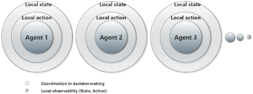
(a) Independent Agents (IAs).

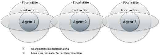
(b) Coordinated reinforcement learning with Max-plus (M+).

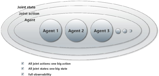
(c) Centralized Agent (CA).

Figure 3: MARL-FWC based on multi-agent and cooperative Q-learning.

4.3 MARL-FWC for adaptive ramp metering plus DSLs

This section illustrates the new conception of ramp metering objective function. This conception takes into account the ramp queue length. This section also demonstrates how DSLs can complement the ramp metering in order to mitigate the traffic congestion when the network is dense.

4.3.1 MARL-FWC another conception of ramp metering objective function

By considering the weighted sum of both freeway density and ramp, it is possible to minimize both the normalized difference from the critical density in the freeway $O_{h}$ and the normalized queue length in the ramp $O_{r}$. The ramp metering objective function $O$ is demonstrated as follows:
Minimize O:

$$O = w_{h}O_{h}+w_{r}O_{r}:$$ Collective Objective Function (17)

$$O_{h} = 2\frac{\left|\rho-\rho_{c}\right|}{\rho_{max}}:$$ Freeway Objective Function

(normalized difference from critical density)

$$O_{r} = \frac{q}{q_{max}}:$$ Ramp Objective Function

(normalized queue length)

$$w_{h} = \frac{\rho\alpha}{\rho_{max}}:$$ Adaptive Freeway Weight

$$w_{r} = \frac{q(1-\alpha)}{q_{max}}:$$ Adaptive Ramp Weight

$$\alpha \in [0,1]:$$ Control Parameter

Where: $w_{h}$ is the adaptive freeway weight. It is adaptive because it depends on the current freeway state; as far as the density increases, the $w_{h}$ also increases. $w_{r}$ is the adaptive ramp weight. It is adaptive because it depends on the current ramp state; as far as the queue length increases, the $w_{r}$ also increases. Finally, $\alpha$ is the control parameter. It is used to determine the importance of each weight (biasing factor). With such conception of ramp metering objective function, there is a balance between mitigating the traffic congestion at the freeway (capacity drop) and moving the problem to another road segment.

4.3.2 DSLs objective function

The DSLs analytical proof proves that changing the velocity affects the freeway density. This section illustrates the analytical proof. This proof is used to demonstrate how the change in velocity can affect both freeway density and flow. It shows that the slope between density and flow is the velocity, see Fig. 4.

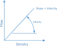
Figure 4: Density, flow and velocity relationship.

$$q = \frac{N}{t}$$ Freeway Flow (veh/h)

$$\rho = \frac{N}{A}=\frac{N}{(d*width(const.))}$$ Freeway Density (veh/km/lane)

$$v = \frac{d}{t}=\frac{{1}/{t}}{{1}/{d}}$$ Freeway Velocity (km/h)

$$~{}\text{Multiply both sides by}~{}N$$

$$v = \frac{{N}/{t}}{{N}/{d}}$$

$$v \propto \frac{q}{\rho}$$ (18)

Where: $N$ is the number of vehicles (veh) (see Fares and Gomaa (2014)) and $t$ is the time (h).

DSLs objective function: taking into account the queue length in designing the freeway objective function Eq. (17) raises a question; how to control the amount of vehicles that enter the merging area from the main stream freeway. Hence, the role of the DSLs can be considered as the main stream metering to complement the ramp metering function. When the ramp metering cannot mitigate the capacity drop at the merging area, the DSLs can complement by limiting the number of vehicles entering the merging area. That been said, the DSLs objective function is as follows:

$$O_{hDSL} = \quad 2\frac{\left|\rho-\rho_{c}\right|}{\rho_{max}},\text{Freeway DSLs Objective Function}$$

(normalized difference from critical density) (19)

4.4 The VISSIM simulation environment

In VISSIM there are many functions and parameters which control the VISSIM itself and associated study experiments. These parameters can be assigned through VISSIM GUI and remain fixed during the running of the experiment or manipulated through programming via VISSIM COM interface which gives the ability to change these parameters during the running time. For example, the traffic signal during the running time of the experiment can be changed in order to respond to the dynamics of the freeway. VISSIM COM interface can be programmed via any type of programming languages with the ability to handle COM object. Accordingly, the next section depicts the advanced VISSIM simulator possibilities, particularly ramp control development and DSLs. Some examples of dense networks with different number of ramps are given, however, MARL-FWC can handle any type of networks with any number of ramps.

5 Performance Evaluation

5.1 Multi-agent reinforcement learning

The studied network in Fig. 5 consists of a mainstream freeway with three lanes and three-metered on-ramp with one lane each. The network consists of four sources of inflow: $O_{1}$ for the mainstream flow, $O_{2},\;O_{3},$ and $O_{4}$ for the three on-ramp flow. It has only one discharge point $D_{1}$ with unrestricted outflow.

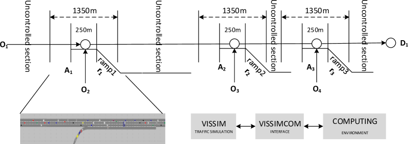
Figure 5: The studied network.

The mainstream freeway consists of three areas of interest: $A_{1}$, $A_{2},$ and $A_{3}$, plus three control agents (RLCA) which are located at the entrance points of each ramp. Each area of interest is associated with one control agent. Each area is about $1350\;m$ as follows: $580\;m$ before the ramp, $250\;m$ as a merging area and $520\;m$ after the ramp. There are four uncontrolled sections; three of them before $A_{1}$, $A_{2}$ (which is about $1500\;m$) and $A_{3}$ (which is about $100\;m$) and the fourth is after $A_{3}$.

Table 1 represents the demand for both the mainstream freeway and ramps. That is because with such scenario the density $\rho$ can exceed the critical density $\rho_{cr}$ which is proven during the learning process. Random choice of action can lead to a scenario with density $\rho$ equals $72$ (Veh/km) which is higher than the critical one $\rho_{cr}$ which is equal to $62$ (Veh/km). The studied network is considered a dense network where the smart control system is highly needed.

Table 1: The demand scenario.

Simulation Time (sec)	300	600	900	1200	1500	1800	2100
Freeway Demand Flow (veh/h)	4000	5500	7000	6500	6000	5500	4500
Ramp Demand Flow (veh/h)	1000	1000	1000	1000	1000	1000	1000

Table 2 shows MARL-FWC performance evaluation per agent (the three approaches), where $A$ is defined as the area of the freeway, which starts from the beginning of $A_{1}$ to the end of $A_{3}$. And $r_{1}$, $r_{2}$, $r_{3}$ are defined as areas starting from the beginning points of the ramps $1$, $2$, and $3$ to the end points of $A_{1}$, $A_{2}$, and $A_{3}$ respectively. In the IAs, $Agent_{1}$ tries greedily to solve its local congestion only regardless of other agents’ problems. This leads to overpopulating section $A_{2}$ of the road, hence increasing the average travel time for $A_{2}$ and $r_{2}$ to $112$ and $113$ respectively, and the same for $Agent_{3}$. In contrary, in coordinated reinforcement learning with Max-plus, the agents optimally cooperate to resolve the congestion problem which leads to 3.2% advance over the IAs case. Although the CA gives some improvements, this costly solution is not recommended compared to the RL with a Max-plus.

Table 2: MARL-FWC performance evaluation per agent.

		$Agent_{1}$		$Agent_{2}$		$Agent_{3}$
		$A_{1}$	$r_{1}$	$A_{2}$	$r_{2}$	$A_{3}$	$r_{3}$	$A$
	IAs	109.05	89.7	112.06	113.07	97.53	80.92	401.79
	Max-plus	112.87	69.18	100.34	77.36	94.18	54.93	388.85
TT(AVG)(s)								3.2%
	CA	110.05	70.47	99.09	77.9	93.68	54.01	385.32
								4%

Line graphs in Fig. 6 demonstrate the freeway density associated with each approach of MARL-FWC over 2100 seconds of simulation. An important thing here is that, in Fig. 6(a), $Agent_{1}$ tries to maintain its density within a small neighborhood of the critical density regardless of other agents’ performance. This leads to overpopulating section $A_{2}$ of the road. Hence, there is a dramatic increase in the density of section $A_{2}$ over the critical ratio between $1400\;s$ and $2100\;s$. This leads to the conclusion that $Agent_{2}$ does not converge to the optimal solution. Figures 6(b) and 6(c) show that coordinated reinforcement learning with Max-plus and centralized agent successfully keep the density of the freeway at required level over the simulation period.

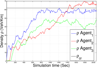
(a) IAs density $\rho$/agent.

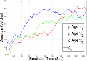
(b) Max-plus density $\rho$/agent.

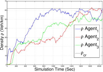
(c) CA density $\rho$/area.

Figure 6: Freeway density for MARL-FWC with the three approaches.

Table 3 provides the results obtained from applying MARL-FWC with all the three approaches and compares it to the base case (no-metering). It can be seen that coordinated reinforcement learning with Max-Plus and centralized agent have shown considerable improvement over the base case. Centralized agent and cooperative $Q$-learning with Max-plus give $6.5$% and $6.9$% in terms of total travel time and $6.74$% and $7.5$% in terms of average speed improvements over the base case, respectively.

Table 3: MARL-FWC performance evaluation.

	No-metering	IAs	Max-plus	Centralized agent
Total travel time (h)	333	331.5	311.5	308.7
		0.5%	6.5%	6.9%
Average speed (km/h)	45.25	45.49	48.5	48.65
		0.5%	6.74%	7.5%

An experiment of a dense network with three ramps is provided, however, MARL-FWC can handle whatsoever type of networks with any number of ramps. In addition, the recommendation for this type of networks and similar ones is to apply the second approach of MARL-FWC which is cooperative $Q$-learning with Max-plus.

5.2 Adaptive objective function plus DSLs

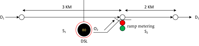
Figure 7: Traffic network with DSLs and a metered on-ramp.

The studied network in Fig. 7 consists of a mainstream freeway with two lanes and an on-ramp with one lane. The network consists of two sources of inflow: $O_{1}$ for the mainstream flow and $O_{2}$ for the on-ramp flow and it has only one discharge point $D_{1}$ with unrestricted outflow. The mainstream freeway consists of two sections: $S_{1}$ and $S_{2}$. The first section $S_{1}$ lies before the ramp, it is $4\;km$ long. The second section $S_{2}$ lies after the ramp, it is $2\;km$ long. The mainstream freeway capacity is $4000\;veh/h$ for both lanes, and the on-ramp capacity is $2000\;veh/h$. The network parameters are taken as follows: $V_{ff}=60\;km^{2}/h$, $\rho(0)=40\;veh/km/lane$, $\rho_{jam}=180\;veh/km/lane$ and $\rho_{cr}=33.5\;veh/km/lane$.

Table 4 represents the demand (for both the mainstream freeway and ramp) considered in the simulation experiment over a four hours period. This demand scenario gives the opportunity to study the effect of the on-ramp smart control and DSLs. In the freeway line, there was an increase in the demand flow over the first hour, then the demand flow remains steady at high level near the capacity of the freeway over two hours and half, and finally, the demand flow decreases in one hour to low level. In the ramp line, the demand flow went up over the first hour, then remains at high level near the capacity for half an hour, finally, it dropped to low value and remains steady for two hours and half. The studied network is considered a dense network where the smart control system is highly needed.

Table 4: Demand scenario for the simulation.

Simulation Time (h)	0.5	1	1.5	2	2.5	3	3.5	4
Freeway Flow (veh/h)	2500	3000	3500	3500	3500	3500	2500	1000
Ramp Flow (veh/h)	500	1000	1500	500	500	500	500	500

Table 5 demonstrates the total time spent (TTS (veh.h.)) between three different strategies. There was a decline in the total time spent, when MARL-FWC for adaptive ramp metering and ramp metering plus DSLs is used as compared to the base case.

Table 5: MARL-FWC for adaptive ramp metering plus DSLs performance evaluation.

	No-metering	Ramp metering	Ramp metering plus DSL
TTS(veh.h.)	1240.0	1152.0 7%	1055.6 14.8%

An important thing to be noticed here is that the new approach for ramp metering plus DSLs have shown considerable improvement over the base case. Adaptive ramp metering and adaptive ramp metering plus DSLs give $7\%$ and $14.8\%$ in terms of total time spent over the base case. Finally, in on-ramp queue constraint, the DSLs can complement the ramp metering by preventing traffic break down and maintaining the traffic flow at high level.

6 Conclusions

In this article, the problem of traffic congestion in freeways at the network level has been addressed. A new system for controlling ramps metering and speed limits has been introduced based on a multi-agent reinforcement-learning framework. MARL-FWC comprises both a MDP modeling technique and an associated cooperative $Q$-learning technique, which is based on payoff propagation (Max-plus algorithm) under the coordination graphs framework. For MARL-FWC to be as optimal as possible, the approach is evaluated using different modes of operation depending on the network architecture. This framework has been tested on the state-of-the-art VISSIM traffic simulator in a dense practical scenarios.

The experimental results have been thoroughly analyzed to study the performance of MARL-FWC using a concrete set of metrics, namely, total travel time, average speed, and total time spent while keeping freeway density at optimum level close to the critical ratio for maximum traffic flow. The findings have proved that MARL-FWC has achieved significant enhancement on three features as compared to the base case. It have been also shown that when the ramp metering could not mitigate the capacity drop at the merging area, DSLs could complement the ramp metering by adjusting the flow rate on the main street via changing the speed limits values. The advantages of applying MARL-FWC include saving car fuel, decreasing air pollution, mitigating capacity drop, and saving lives by reducing the chances of car accidents.

7 Acknowledgements

This work is mainly supported by the Ministry of Higher Education (MoHE) of Egypt through PhD fellowship awarded to Dr. Ahmed Fares. This work is supported in part by the Science and Technology Development Fund (STDF), Project ID 12602 ”Integrated Traffic Management and Control System”, and by E-JUST Research Fellowship awarded to Dr. Mohamed A. Khamis.

References

- Bertsekas (1996) Bertsekas DP. Dynamic programming and optimal control, vol. 1. Athena Scientific Belmont, Massachusetts; 1996.
- Ernst et al. (2009) Ernst D, Glavic M, Capitanescu F, Wehenkel L. Reinforcement learning versus model predictive control: a comparison on a power system problem. Systems, Man, and Cybernetics, Part B: Cybernetics, IEEE Transactions on 2009;39(2):517–529.
- Fares and Gomaa (2014) Fares A, Gomaa W. Freeway ramp-metering control based on Reinforcement learning. In: Control Automation (ICCA), 11th IEEE International Conference on; 2014. p. 1226–1231.
- Fares and Gomaa (2015) Fares A, Gomaa W. Multi-Agent Reinforcement Learning Control for Ramp Metering. In: Selvaraj H, Zydek D, Chmaj G, editors. Progress in Systems Engineering, vol. 330 of Advances in Intelligent Systems and Computing Springer International Publishing; 2015.p. 167–173.
- Feng et al. (2011) Feng C, Yuanhua J, Jian L, Huixin Y, Zhonghai N. Design of Fuzzy Neural Network Control Method for Ramp Metering. In: Measuring Technology and Mechatronics Automation (ICMTMA), 2011 Third International Conference on, vol. 1; 2011. p. 966–969.
- Ghods et al. (2009) Ghods AH, Kian A, Tabibi M. Adaptive freeway ramp metering and variable speed limit control: a genetic-fuzzy approach. Intelligent Transportation Systems Magazine, IEEE 2009;1(1):27–36.
- Guestrin et al. (2001) Guestrin C, Koller D, Parr R. Multiagent planning with factored MDPs. In: NIPS, vol. 1; 2001. p. 1523–1530.
- Guestrin (2003) Guestrin CE. Planning under uncertainty in complex structured environments. PhD thesis, Stanford University; 2003.
- Kaelbling and Moore (1996) Kaelbling MLL Leslie Pack, Moore AW. Reinforcement learning: A survey. Journal of artificial intelligence research 1996;p. 237–285.
- Khamis and Gomaa (2012) Khamis MA, Gomaa W. Enhanced Multiagent Multi-Objective Reinforcement Learning for Urban Traffic Light Control. In: Proc. IEEE 11th International Conference on Machine Learning and Applications (ICMLA 2012) Boca Raton, Florida; 2012. p. 586–591.
- Khamis and Gomaa (2014) Khamis MA, Gomaa W. Adaptive multi-objective reinforcement learning with hybrid exploration for traffic signal control based on cooperative multi-agent framework. Journal of Engineering Applications of Artificial Intelligence 2014 March;29:134–151.
- Khamis and Gomaa (2015) Khamis MA, Gomaa W. Comparative Assessment of Machine-Learning Scoring Functions on PDBbind 2013. Engineering Applications of Artificial Intelligence 2015;p. 136–151.
- Khamis et al. (2015) Khamis MA, Gomaa W, Ahmed WF. Machine learning in computational docking. Artificial Intelligence In Medicine 2015;63:135–152.
- Khamis et al. (2012a) Khamis MA, Gomaa W, El-Mahdy A, Shoukry A. Adaptive Traffic Control System Based on Bayesian Probability Interpretation. In: Proc. IEEE 2012 Japan-Egypt Conference on Electronics, Communications and Computers (JEC-ECC 2012) Alexandria, Egypt; 2012. p. 151–156.
- Khamis et al. (2012b) Khamis MA, Gomaa W, El-Shishiny H. Multi-Objective Traffic Light Control System based on Bayesian Probability Interpretation. In: Proc. IEEE 15th International Conference on Intelligent Transportation Systems (ITSC 2012) Anchorage, AK; 2012. p. 995–1000.
- Kok and Vlassis (2006) Kok JR, Vlassis N. Collaborative multiagent reinforcement learning by payoff propagation. The Journal of Machine Learning Research 2006;7:1789–1828.
- Kschischang et al. (2001) Kschischang FR, Frey BJ, Loeliger HA. Factor graphs and the sum-product algorithm. Information Theory, IEEE Transactions on 2001;47(2):498–519.
- Li and Liang (2009) Li J, Liang X. Freeway ramp control based on single neuron. In: Intelligent Computing and Intelligent Systems, 2009. ICIS 2009. IEEE International Conference on, vol. 2; 2009. p. 122–125.
- Liang et al. (2010) Liang X, Li J, Luo N. Single Neuron Based Freeway Traffic Density Control via Ramp Metering. In: Information Engineering and Computer Science (ICIECS), 2010 2nd International Conference on; 2010. p. 1–4.
- Papageorgiou et al. (1991) Papageorgiou M, Hadj-Salem H, Blosseville JM. ALINEA: A local feedback control law for on-ramp metering. Transportation Research Record 1991;(1320).
- Pearl (1988) Pearl J. Probabilistic reasoning in intelligent systems: networks of plausible inference. Morgan Kaufmann; 1988.
- Prendinger et al. (2013) Prendinger H, Gajananan K, Bayoumy Zaki A, Fares A, Molenaar R, Urbano D, et al. Tokyo Virtual Living Lab: Designing Smart Cities Based on the 3D Internet. Internet Computing, IEEE 2013 Nov;17(6):30–38.
- Vlassis et al. (2004) Vlassis N, Elhorst R, Kok JR. Anytime algorithms for multiagent decision making using coordination graphs. In: Systems, Man and Cybernetics, 2004 IEEE International Conference on, vol. 1 IEEE; 2004. p. 953–957.
- Wainwright et al. (2004) Wainwright M, Jaakkola T, Willsky A. Tree consistency and bounds on the performance of the max-product algorithm and its generalizations. Statistics and Computing 2004;14(2):143–166.
- Watkins and Dayan (1992) Watkins CJ, Dayan P. Q-learning. Machine learning 1992;8(3-4):279–292.
- Yedidia et al. (2003) Yedidia JS, Freeman WT, Weiss Y. Understanding belief propagation and its generalizations. Exploring artificial intelligence in the new millennium 2003;8:236–239.
- Yu et al. (2012) Yu XF, Xu WL, Alam F, Potgieter J, Fang CF. Genetic fuzzy logic approach to local ramp metering control using microscopic traffic simulation. In: Mechatronics and Machine Vision in Practice (M2VIP), 2012 19th International Conference; 2012. p. 290–297.
- Zaky et al. (2015) Zaky AB, Gomaa W, Khamis MA. Car Following Markov Regime Classification and Calibration. In: Proceedings of the IEEE 14th International Conference on Machine Learning and Applications (ICMLA 2015) Miami, Florida, USA: IEEE; 2015. .