Self-Attentive Sequential Recommendation

Abstract

Sequential dynamics are a key feature of many modern recommender systems, which seek to capture the ‘context’ of users’ activities on the basis of actions they have performed recently. To capture such patterns, two approaches have proliferated: Markov Chains (MCs) and Recurrent Neural Networks (RNNs). Markov Chains assume that a user’s next action can be predicted on the basis of just their last (or last few) actions, while RNNs in principle allow for longer-term semantics to be uncovered. Generally speaking, MC-based methods perform best in extremely sparse datasets, where model parsimony is critical, while RNNs perform better in denser datasets where higher model complexity is affordable. The goal of our work is to balance these two goals, by proposing a self-attention based sequential model (SASRec) that allows us to capture long-term semantics (like an RNN), but, using an attention mechanism, makes its predictions based on relatively few actions (like an MC). At each time step, SASRec seeks to identify which items are ‘relevant’ from a user’s action history, and use them to predict the next item. Extensive empirical studies show that our method outperforms various state-of-the-art sequential models (including MC/CNN/RNN-based approaches) on both sparse and dense datasets. Moreover, the model is an order of magnitude more efficient than comparable CNN/RNN-based models. Visualizations on attention weights also show how our model adaptively handles datasets with various density, and uncovers meaningful patterns in activity sequences.

I Introduction

The goal of sequential recommender systems is to combine personalized models of user behavior (based on historical activities) with some notion of ‘context’ on the basis of users’ recent actions. Capturing useful patterns from sequential dynamics is challenging, primarily because the dimension of the input space grows exponentially with the number of past actions used as context. Research in sequential recommendation is therefore largely concerned with how to capture these high-order dynamics succinctly.

Markov Chains (MCs) are a classic example, which assume that the next action is conditioned on only the previous action (or previous few), and have been successfully adopted to characterize short-range item transitions for recommendation [1]. Another line of work uses Recurrent Neural Networks (RNNs) to summarize all previous actions via a hidden state, which is used to predict the next action [2].

Both approaches, while strong in specific cases, are somewhat limited to certain types of data. MC-based methods, by making strong simplifying assumptions, perform well in high-sparsity settings, but may fail to capture the intricate dynamics of more complex scenarios. Conversely RNNs, while expressive, require large amounts of data (an in particular dense data) before they can outperform simpler baselines.

Recently, a new sequential model Transfomer achieved state-of-the-art performance and efficiency for machine translation tasks [3]. Unlike existing sequential models that use convolutional or recurrent modules, Transformer is purely based on a proposed attention mechanism called ‘self-attention,’ which is highly efficient and capable of uncovering syntactic and semantic patterns between words in a sentence.

Inspired by this method, we seek to apply self-attention mechanisms to sequential recommendation problems. Our hope is that this idea can address both of the problems outlined above, being on the one hand able to draw context from all actions in the past (like RNNs) but on the other hand being able to frame predictions in terms of just a small number of actions (like MCs). Specifically, we build a Self-Attention based Sequential Recommendation model (SASRec), which adaptively assigns weights to previous items at each time step (Figure 1).

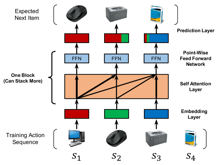
Figure 1: A simplified diagram showing the training process of SASRec. At each time step, the model considers all previous items, and uses attention to ‘focus on’ items relevant to the next action.

The proposed model significantly outperforms state-of-the-art MC/CNN/RNN-based sequential recommendation methods on several benchmark datasets. In particular, we examine performance as a function of dataset sparsity, where model performance aligns closely with the patterns described above. Due to the self-attention mechanism, SASRec tends to consider long-range dependencies on dense datasets, while focusing on more recent activities on sparse datasets. This proves crucial for adaptively handling datasets with varying density.

Furthermore, the core component (i.e., the self-attention block) of SASRec is suitable for parallel acceleration, resulting in a model that is an order of magnitude faster than CNN/RNN-based alternatives. In addition, we analyze the complexity and scalability of SASRec, conduct a comprehensive ablation study to show the effect of key components, and visualize the attention weights to qualitatively reveal the model’s behavior.

II Related Work

Several lines of work are closely related to ours. We first discuss general, followed by temporal, recommendation, before discussing sequential recommendation (in particular MCs and RNNs). Last we introduce the attention mechanism, especially the self-attention module which is at the core of our model.

II-A General Recommendation

Recommender systems focus on modeling the compatibility between users and items, based on historical feedback (e.g. clicks, purchases, likes). User feedback can be explicit (e.g. ratings) or implicit (e.g. clicks, purchases, comments) [4, 5]. Modeling implicit feedback can be challenging due to the ambiguity of interpreting ‘non-observed’ (e.g. non-purchased) data. To address the problem, point-wise [4] and pairwise [5] methods are proposed to solve such challenges.

Matrix Factorization (MF) methods seek to uncover latent dimensions to represent users’ preferences and items’ properties, and estimate interactions through the inner product between the user and item embeddings [6, 7]. In addition, another line of work is based on Item Similarity Models (ISM) and doesn’t explicitly model each user with latent factors (e.g. FISM [8]). They learn an item-to-item similarity matrix, and estimate a user’s preference toward an item via measuring its similarities with items that the user has interacted with before.

Recently, due to their success in related problems, various deep learning techniques have been introduced for recommendation [9]. One line of work seeks to use neural networks to extract item features (e.g. images [10, 11], text [12, 13], etc.) for content-aware recommendation. Another line of work seeks to replace conventional MF. For example, NeuMF [14] estimates user preferences via Multi-Layer Perceptions (MLP), and AutoRec [15] predicts ratings using autoencoders.

II-B Temporal Recommendation

Dating back to the Netflix Prize, temporal recommendation has shown strong performance on various tasks by explicitly modeling the timestamp of users’ activities. TimeSVD++ [16] achieved strong results by splitting time into several segments and modeling users and items separately in each. Such models are essential to understand datasets that exhibit significant (short- or long-term) temporal ‘drift’ (e.g. ‘how have movie preferences changed in the last 10 years,’ or ‘what kind of businesses do users visit at 4pm?’, etc.) [17, 18, 16]. Sequential recommendation (or next-item recommendation) differs slightly from this setting, as it only considers the order of actions, and models sequential patterns which are independent of time. Essentially, sequential models try to model the ‘context’ of users’ actions based on their recent activities, rather than considering temporal patterns per se.

II-C Sequential Recommendation

Many sequential recommender systems seek to model item-item transition matrices as a means of capturing sequential patterns among successive items. For instance, FPMC fuses an MF term and an item-item transition term to capture long-term preferences and short-term transitions respectively [1]. Essentially, the captured transition is a first-order Markov Chain (MC), whereas higher-order MCs assume the next action is related to several previous actions. Since the last visited item is often the key factor affecting the user’s next action (essentially providing ‘context’), first-order MC based methods show strong performance, especially on sparse datasets [19]. There are also methods adopting high-order MCs that consider more previous items [20, 21]. In particular, Convolutional Sequence Embedding (Caser), a CNN-based method, views the embedding matrix of $L$ previous items as an ‘image’ and applies convolutional operations to extract transitions [22].

Other than MC-based methods, another line of work adopts RNNs to model user sequences [23, 2, 24, 25]. For example, GRU4Rec uses Gated Recurrent Units (GRU) to model click sequences for session-based recommendation [2], and an improved version further boosts its Top-N recommendation performance [26]. In each time step, RNNs take the state from the last step and current action as its input. These dependencies make RNNs less efficient, though techniques like ‘session-parallelism’ have been proposed to improve efficiency [2].

II-D Attention Mechanisms

Attention mechanisms have been shown to be effective in various tasks such as image captioning [27] and machine translation [28], among others. Essentially the idea behind such mechanisms is that sequential outputs (for example) each depend on ‘relevant’ parts of some input that the model should focus on successively. An additional benefit is that attention-based methods are often more interpretable. Recently, attention mechanisms have been incorporated into recommender systems [29, 30, 31]. For example, Attentional Factorization Machines (AFM) [30] learn the importance of each feature interaction for content-aware recommendation.

However, the attention technique used in the above is essentially an additional component to the original model (e.g. attention+RNNs, attention+FMs, etc.). Recently, a purely attention-based sequence-to-sequence method, Transfomer [3], achieved state-of-the-art performance and efficiency on machine translation tasks which had previously been dominated by RNN/CNN-based approaches [32, 33]. The Transformer model relies heavily on the proposed ‘self-attention’ modules to capture complex structures in sentences, and to retrieve relevant words (in the source language) for generating the next word (in the target language). Inspired by Transformer, we seek to build a new sequential recommendation model based upon the self-attention approach, though the problem of sequential recommendation is quite different from machine translation, and requires specially designed models.

III Methodology

Table I: Notation.

Notation	Description
$\mathcal{U},\mathcal{I}$	user and item set
$\mathcal{S}^{u}$	historical interaction sequence for a user $u$: $(\mathcal{S}^{u}_{1},\mathcal{S}^{u}_{2},...,\mathcal{S}^{u}_{|\mathcal{S}^{u}|})$
$d\in\mathbb{N}$	latent vector dimensionality
$n\in\mathbb{N}$	maximum sequence length
$b\in\mathbb{N}$	number of self-attention blocks
${\bf M}\in\mathbb{R}^{|\mathcal{I}|\times d}$	item embedding matrix
${\bf P}\in\mathbb{R}^{n\times d}$	positional embedding matrix
$\widehat{{\bf E}}\in\mathbb{R}^{n\times d}$	input embedding matrix
${\bf S}^{(b)}\in\mathbb{R}^{n\times d}$	item embeddings after the $b$-th self-attention layer
${\bf F}^{(b)}\in\mathbb{R}^{n\times d}$	item embeddings after the $b$-th feed-forward network

In the setting of sequential recommendation, we are given a user’s action sequence $\mathcal{S}^{u}=(\mathcal{S}^{u}_{1},\mathcal{S}^{u}_{2},\ldots,\mathcal{S}^{u}_{|\mathcal{S}^{u}|})$, and seek to predict the next item. During the training process, at time step $t$, the model predicts the next item depending on the previous $t$ items. As shown in Figure 1, it will be convenient to think of the model’s input as $(\mathcal{S}^{u}_{1},\mathcal{S}^{u}_{2},\ldots,\mathcal{S}^{u}_{|\mathcal{S}^{u}|-1})$ and its expected output as a ‘shifted’ version of the same sequence: $(\mathcal{S}^{u}_{2},\mathcal{S}^{u}_{3},\ldots,\mathcal{S}^{u}_{|\mathcal{S}^{u}|})$. In this section, we describe how we build a sequential recommendation model via an embedding layer, several self-attention blocks, and a prediction layer. We also analyze its complexity and further discuss how SASRec differs from related models. Our notation is summarized in Table I.

III-A Embedding Layer

We transform the training sequence $(\mathcal{S}^{u}_{1},\mathcal{S}^{u}_{2},...,\mathcal{S}^{u}_{|\mathcal{S}^{u}|-1})$ into a fixed-length sequence $s=(s_{1},s_{2},\dots,s_{n})$, where $n$ represents the maximum length that our model can handle. If the sequence length is greater than $n$, we consider the most recent $n$ actions. If the sequence length is less than $n$, we repeatedly add a ‘padding’ item to the left until the length is $n$. We create an item embedding matrix ${\bf M}\in\mathbb{R}^{|\mathcal{I}|\times d}$ where $d$ is the latent dimensionality, and retrieve the input embedding matrix ${\bf E}\in\mathbb{R}^{n\times d}$, where ${\bf E}_{i}={\bf M}_{s_{i}}$. A constant zero vector ${\bf 0}$ is used as the embedding for the padding item.

Positional Embedding

As we will see in the next section, since the self-attention model doesn’t include any recurrent or convolutional module, it is not aware of the positions of previous items. Hence we inject a learnable position embedding ${\bf P}\in\mathbb{R}^{n\times d}$ into the input embedding:

$$\widehat{{\bf E}}=\left[\begin{tabular}[]{c}${\bf M}_{s_{1}}+{\bf P}_{1}$\\ ${\bf M}_{s_{2}}+{\bf P}_{2}$\\ $\dots$\\ ${\bf M}_{s_{n}}+{\bf P}_{n}$\end{tabular}\right]$$ (1)

We also tried the fixed position embedding as used in [3], but found that this led to worse performance in our case. We analyze the effect of the position embedding quantitatively and qualitatively in our experiments.

III-B Self-Attention Block

The scaled dot-product attention [3] is defined as:

$$\text{Attention}({\bf Q},{\bf K},{\bf V})=\text{softmax}\left(\frac{{\bf Q}{\bf K}^{T}}{\sqrt{d}}\right){\bf V},$$ (2)

where ${\bf Q}$ represents the queries, ${\bf K}$ the keys and ${\bf V}$ the values (each row represents an item). Intuitively, the attention layer calculates a weighted sum of all values, where the weight between query $i$ and value $j$ relates to the interaction between query $i$ and key $j$. The scale factor $\sqrt{d}$ is to avoid overly large values of the inner product, especially when the dimensionality is high.

Self-Attention layer

In NLP tasks such as machine translation, attention mechanisms are typically used with ${\bf K}={\bf V}$ (e.g. using an RNN encoder-decoder for translation: the encoder’s hidden states are keys and values, and the decoder’s hidden states are queries) [28]. Recently, a self-attention method was proposed which uses the same objects as queries, keys, and values [3]. In our case, the self-attention operation takes the embedding $\widehat{{\bf E}}$ as input, converts it to three matrices through linear projections, and feeds them into an attention layer:

$${\bf S}=\text{SA}(\widehat{{\bf E}})=\text{Attention}(\widehat{{\bf E}}{\bf W}^{Q},\widehat{{\bf E}}{\bf W}^{K},\widehat{{\bf E}}{\bf W}^{V}),$$ (3)

where the projection matrices ${\bf W}^{Q},{\bf W}^{K},{\bf W}^{V}\in\mathbb{R}^{d\times d}$. The projections make the model more flexible. For example, the model can learn asymmetric interactions (i.e., <query $i$, key $j$> and <query $j$, key $i$> can have different interactions).

Causality

Due to the nature of sequences, the model should consider only the first $t$ items when predicting the $(t+1)$-st item. However, the $t$-th output of the self-attention layer (${\bf S}_{t}$) contains embeddings of subsequent items, which makes the model ill-posed. Hence, we modify the attention by forbidding all links between ${\bf Q}_{i}$ and ${\bf K}_{j}$ ($j>i$).

Point-Wise Feed-Forward Network

Though the self-attention is able to aggregate all previous items’ embeddings with adaptive weights, ultimately it is still a linear model. To endow the model with nonlinearity and to consider interactions between different latent dimensions, we apply a point-wise two-layer feed-forward network to all ${\bf S}_{i}$ identically (sharing parameters):

$${\bf F}_{i}=\text{FFN}({\bf S}_{i})=\text{ReLU}({\bf S}_{i}{\bf W}^{(1)}+{\bf b}^{(1)}){\bf W}^{(2)}+{\bf b}^{(2)},$$ (4)

where ${\bf W}^{(1)},{\bf W}^{(2)}$ are $d\times d$ matrices and ${\bf b}^{(1)},{\bf b}^{(2)}$ are $d$-dimensional vectors. Note that there is no interaction between ${\bf S}_{i}$ and ${\bf S}_{j}$ ($i\neq j$), meaning that we still prevent information leaks (from back to front).

III-C Stacking Self-Attention Blocks

After the first self-attention block, ${\bf F}_{i}$ essentially aggregates all previous items’ embeddings (i.e., $\widehat{{\bf E}}_{j},j\leq i$). However, it might be useful to learn more complex item transitions via another self-attention block based on ${\bf F}$. Specifically, we stack the self-attention block (i.e., a self-attention layer and a feed-forward network), and the $b$-th ($b>1$) block is defined as:

$$\begin{array}[]{c}{\bf S}^{(b)}=\text{SA}({\bf F}^{(b-1)}),\\ {\bf F}_{i}^{(b)}=\text{FFN}({\bf S}_{i}^{(b)}),\ \ \forall i\in\{1,2,\dots,n\},\end{array}$$ (5)

and the $1$-st block is defined as ${\bf S}^{(1)}={\bf S}$ and ${\bf F}^{(1)}={\bf F}$.

However, when the network goes deeper, several problems become exacerbated: 1) the increased model capacity leads to overfitting; 2) the training process becomes unstable (due to vanishing gradients etc.); and 3) models with more parameters often require more training time. Inspired by [3], We perform the following operations to alleviate these problems:

$$g(x)=x+\text{Dropout}(g(\text{LayerNorm}(x))),$$

where $g(x)$ represents the self attention layer or the feed-forward network. That is to say, for layer $g$ in each block, we apply layer normalization on the input $x$ before feeding into $g$, apply dropout on $g$’s output, and add the input $x$ to the final output. We introduce these operations below.

Residual Connections

In some cases, multi-layer neural networks have demonstrated the ability to learn meaningful features hierarchically [34]. However, simply adding more layers did not easily correspond to better performance until residual networks were proposed [35]. The core idea behind residual networks is to propagate low-layer features to higher layers by residual connection. Hence, if low-layer features are useful, the model can easily propagate them to the final layer. Similarly, we assume residual connections are also useful in our case. For example, existing sequential recommendation methods have shown that the last visited item plays a key role on predicting the next item [1, 21, 19]. However, after several self-attention blocks, the embedding of the last visited item is entangled with all previous items; adding residual connections to propagate the last visited item’s embedding to the final layer would make it much easier for the model to leverage low-layer information.

Layer Normalization

Layer normalization is used to normalize the inputs across features (i.e., zero-mean and unit-variance), which is beneficial for stabilizing and accelerating neural network training [36]. Unlike batch normalization [37], the statistics used in layer normalization are independent of other samples in the same batch. Specifically, assuming the input is a vector ${\bf x}$ which contains all features of a sample, the operation is defined as:

$$\text{LayerNorm}({\bf x})=\bm{\alpha}\odot\frac{{\bf x}-\mu}{\sqrt{\sigma^{2}+\epsilon}}+\bm{\beta},$$

where $\odot$ is an element-wise product (i.e., the Hadamard product), $\mu$ and $\sigma$ are the mean and variance of ${\bf x}$, $\bm{\alpha}$ and $\bm{\beta}$ are learned scaling factors and bias terms.

Dropout

To alleviate overfitting problems in deep neural networks, ‘Dropout’ regularization techniques have been shown to be effective in various neural network architectures [38]. The idea of dropout is simple: randomly ‘turn off’ neurons with probability $p$ during training, and use all neurons when testing. Further analysis points out that dropout can be viewed as a form of ensemble learning which considers an enormous number of models (exponential in the number of neurons and input features) that share parameters [39]. We also apply a dropout layer on the embedding $\widehat{{\bf E}}$.

III-D Prediction Layer

After $b$ self-attention blocks that adaptively and hierarchically extract information of previously consumed items, we predict the next item (given the first $t$ items) based on ${\bf F}_{t}^{(b)}$. Specifically, we adopt an MF layer to predict the relevance of item $i$:

$$r_{i,t}={\bf F}_{t}^{(b)}{\bf N}_{i}^{T},$$

where $r_{i,t}$ is the relevance of item $i$ being the next item given the first $t$ items (i.e., $s_{1},s_{2},\ldots,s_{t}$), and ${\bf N}\in\mathbb{R}^{|\mathcal{I}|\times d}$ is an item embedding matrix. Hence, a high interaction score $r_{i,t}$ means a high relevance, and we can generate recommendations by ranking the scores.

Shared Item Embedding

To reduce the model size and alleviate overfitting, we consider another scheme which only uses a single item embedding ${\bf M}$:

$$r_{i,t}={\bf F}_{t}^{(b)}{\bf M}_{i}^{T}.$$ (6)

Note that ${\bf F}_{t}^{(b)}$ can be represented as a function depending on the item embedding ${\bf M}$: ${\bf F}_{t}^{(b)}=f({\bf M}_{s_{1}},{\bf M}_{s_{2}},\dots,{\bf M}_{s_{t}})$. A potential issue of using homogeneous item embeddings is that their inner products cannot represent asymmetric item transitions (e.g. item $i$ is frequently bought after $j$, but not vise versa), and thus existing methods like FPMC tend to use heterogeneous item embeddings. However, our model doesn’t have this issue since it learns a nonlinear transformation. For example, the feed forward network can easily achieve the asymmetry with the same item embedding: $\text{FFN}({\bf M}_{i}){\bf M}_{j}^{T}\neq\text{FFN}({\bf M}_{j}){\bf M}_{i}^{T}$. Empirically, using a shared item embedding significantly improves the performance of our model.

Explicit User Modeling

To provide personalized recommendations, existing methods often take one of two approaches: 1) learn an explicit user embedding representing user preferences (e.g. MF [40], FPMC [1] and Caser [22]); 2) consider the user’s previous actions, and induce an implicit user embedding from embeddings of visited items (e.g. FSIM [8], Fossil [21], GRU4Rec [2]). Our method falls into the latter category, as we generate an embedding ${\bf F}^{(b)}_{n}$ by considering all actions of a user. However, we can also insert an explicit user embedding at the last layer, for example via addition: $r_{u,i,t}=({\bf U}_{u}+{\bf F}_{t}^{(b)}){\bf M}_{i}^{T}$ where ${\bf U}$ is a user embedding matrix. However, we empirically find that adding an explicit user embedding doesn’t improve performance (presumably because the model already considers all of the user’s actions).

III-E Network Training

Recall that we convert each user sequence (excluding the last action) $(\mathcal{S}^{u}_{1},\mathcal{S}^{u}_{2},\ldots,\mathcal{S}^{u}_{|\mathcal{S}^{u}|-1})$ to a fixed length sequence $s=\{s_{1},s_{2},\dots,s_{n}\}$ via truncation or padding items. We define $o_{t}$ as the expected output at time step $t$:

$$o_{t}=\begin{cases}\texttt{<pad>}&\text{if }s_{t}\text{ is a padding item}\\ s_{t+1}&1\leq t<n\\ \mathcal{S}^{u}_{|\mathcal{S}^{u}|}&t=n\end{cases},$$

where <pad> indicates a padding item. Our model takes a sequence $s$ as input, the corresponding sequence $o$ as expected output, and we adopt the binary cross entropy loss as the objective function:

$$-\sum_{\mathcal{S}^{u}\in\mathcal{S}}\sum_{t\in[1,2,\dots,n]}\left[\log(\sigma(r_{o_{t},t}))+\sum_{j\not\in\mathcal{S}^{u}}\log(1-\sigma(r_{j,t}))\right].$$

Note that we ignore the terms where $o_{t}=\texttt{<pad>}$.

The network is optimized by the Adam optimizer [41], which is a variant of Stochastic Gradient Descent (SGD) with adaptive moment estimation. In each epoch, we randomly generate one negative item $j$ for each time step in each sequence. More implementation details are described later.

III-F Complexity Analysis

Space Complexity

The learned parameters in our model are from the embeddings and parameters in the self-attention layers, feed-forward networks and layer normalization. The total number of parameters is $O(|\mathcal{I}|d+nd+d^{2})$, which is moderate compared to other methods (e.g. $O(|\mathcal{U}|d+|\mathcal{I}|d)$ for FPMC) since it does not grow with the number of users, and $d$ is typically small in recommendation problems.

Time Complexity

The computational complexity of our model is mainly due to the self-attention layer and the feed-forward network, which is $O(n^{2}d+nd^{2})$. The dominant term is typically $O(n^{2}d)$ from the self-attention layer. However, a convenient property in our model is that the computation in each self-attention layer is fully parallelizable, which is amenable to GPU acceleration. In contrast, RNN-based methods (e.g. GRU4Rec [2]) have a dependency on time steps (i.e., computation on time step $t$ must wait for results from time step $t\text{-}1$), which leads to an $O(n)$ time on sequential operations. We empirically find our method is over ten times faster than RNN and CNN-based methods with GPUs (the result is similar to that in [3] for machine translation tasks), and the maximum length $n$ can easily scale to a few hundred which is generally sufficient for existing benchmark datasets.

During testing, for each user, after calculating the embedding ${\bf F}_{n}^{(b)}$ , the process is the same as standard MF methods. ($O(d)$ for evaluating the preference toward an item).

Handing Long Sequences

Though our experiments empirically verify the efficiency of our method, ultimately it cannot scale to very long sequences. A few options are promising to investigate in the future: 1) using restricted self-attention [42] which only attends on recent actions rather than all actions, and distant actions can be considered in higher layers; 2) splitting long sequences into short segments as in [22].

III-G Discussion

We find that SASRec can be viewed as a generalization of some classic CF models. We also discuss conceptually how our approach and existing methods handle sequence modeling.

Reduction to Existing Models

• Factorized Markov Chains: FMC factorizes a first-order item transition matrix, and predicts the next item $j$ depending on the last item $i$:

  $$P(j|i)\propto{\bf M}_{i}^{T}{\bf N}_{j}.$$

  If we set the self-attention block to zero, use unshared item embeddings, and remove the position embedding, SASRec reduces to FMC. Furthermore, SASRec is also closely related to Factorized Personalized Markov Chains (FPMC) [1], which fuse MF with FMC to capture user preferences and short-term dynamics respectively:

  $$P(j|u,i)\propto\left[{\bf U}_{u},{\bf M}_{i}\right]{\bf N}^{T}_{j}.$$

  Following the reduction operations above for FMC, and adding an explicit user embedding (via concatenation), SASRec is equivalent to FPMC.

• Factorized Item Similarity Models [8]: FISM estimates a preference score toward item $i$ by considering the similarities between $i$ and items the user consumed before:

  $$P(j|u)\propto\left(\frac{1}{|\mathcal{S}^{u}|}\sum_{i\in\mathcal{S}^{u}}{\bf M}_{i}\right){\bf N}^{T}_{j}.$$

  If we use one self-attention layer (excluding the feed-forward network), set uniform attention weights (i.e., $\frac{1}{|\mathcal{S}_{u}|}$) on items, use unshared item embeddings, and remove the position embedding, SASRec is reduced to FISM. Thus our model can be viewed as an adaptive, hierarchical, sequential item similarity model for next item recommendation.

MC-based Recommendation

Markov Chains (MC) can effectively capture local sequential patterns, assuming that the next item is only dependent on the previous $L$ items. Exiting MC-based sequential recommendation methods rely on either first-order MCs (e.g. FPMC [1], HRM [43], TransRec [19]) or high-order MCs (e.g. Fossil [21], Vista [20], Caser [22]). The first group of methods tend to perform best on sparse datasets. In contrast, higher-order MC based methods have two limitations: (1) The MC order $L$ needs to be specified before training, rather than being chosen adaptively; (2) The performance and efficiency doesn’t scale well with the order $L$, hence $L$ is typically small (e.g. less than 5). Our method resolves the first issue, since it can adaptively attend on related previous items (e.g. focusing on just the last item on sparse dataset, and more items on dense datasets). Moreover, our model is essentially conditioned on $n$ previous items, and can empirically scale to several hundred previous items, exhibiting performance gains with moderate increases in training time.

RNN-based Recommendation

Another line of work seeks to use RNNs to model user action sequences [2, 26, 17]. RNNs are generally suitable for modeling sequences, though recent studies show CNNs and self-attention can be stronger in some sequential settings [3, 44]. Our self-attention based model can be derived from item similarity models, which are a reasonable alternative for sequence modeling for recommendation. For RNNs, other than their inefficiency in parallel computation (Section III-F), their maximum path length (from an input node to related output nodes) is $O(n)$. In contrast, our model has $O(1)$ maximum path length, which can be beneficial for learning long-range dependencies [45].

IV Experiments

In this section, we present our experimental setup and empirical results. Our experiments are designed to answer the following research questions:

RQ1:

Does SASRec outperform state-of-the-art models including CNN/RNN based methods?

RQ2:

What is the influence of various components in the SASRec architecture?

RQ3:

What is the training efficiency and scalability (regarding $n$) of SASRec?

RQ4:

Are the attention weights able to learn meaningful patterns related to positions or items’ attributes?

IV-A Datasets

We evaluate our methods on four datasets from three real world applications. The datasets vary significantly in domains, platforms, and sparsity:

• Amazon: A series of datasets introduced in [46], comprising large corpora of product reviews crawled from Amazon.com. Top-level product categories on Amazon are treated as separate datasets. We consider two categories, ‘Beauty,’ and ‘Games.’ This dataset is notable for its high sparsity and variability.

• Steam: We introduce a new dataset crawled from Steam, a large online video game distribution platform. The dataset contains 2,567,538 users, 15,474 games and 7,793,069 English reviews spanning October 2010 to January 2018. The dataset also includes rich information that might be useful in future work, like users’ play hours, pricing information, media score, category, developer (etc.).

• MovieLens: A widely used benchmark dataset for evaluating collaborative filtering algorithms. We use the version (MovieLens-1M) that includes 1 million user ratings.

We followed the same preprocessing procedure from [19, 21, 1]. For all datasets, we treat the presence of a review or rating as implicit feedback (i.e., the user interacted with the item) and use timestamps to determine the sequence order of actions. We discard users and items with fewer than 5 related actions. For partitioning, we split the historical sequence $\mathcal{S}^{u}$ for each user $u$ into three parts: (1) the most recent action $\mathcal{S}^{u}_{|\mathcal{S}^{u}|}$ for testing, (2) the second most recent action $\mathcal{S}^{u}_{|\mathcal{S}^{u}|-1}$ for validation, and (3) all remaining actions for training. Note that during testing, the input sequences contain training actions and the validation action.

Data statistics are shown in Table II. We see that the two Amazon datasets have the fewest actions per user and per item (on average), Steam has a high average number of actions per item, and MovieLens-1m is the most dense dataset.

Table II: Dataset statistics (after preprocessing)

Dataset	#users	#items	avg. actions /user	avg. actions /item	#actions
Amazon Beauty	52,024	57,289	7.6	6.9	0.4M
Amazon Games	31,013	23,715	9.3	12.1	0.3M
Steam	334,730	13,047	11.0	282.5	3.7M
MovieLens-1M	6,040	3,416	163.5	289.1	1.0M

Table III: Recommendation performance. The best performing method in each row is boldfaced, and the second best method in each row is underlined. Improvements over non-neural and neural approaches are shown in the last two columns respectively.

Dataset	Metric	(a) PopRec	(b) BPR	(c) FMC	(d) FPMC	(e) TransRec	(f) GRU4Rec	(g) GRU4Rec${}^{\texttt{+}}$	(h) Caser	(i) SASRec	Improvement vs.
											(a)-(e)	(f)-(h)
Beauty	Hit@10	0.4003	0.3775	0.3771	0.4310	0.4607	0.2125	0.3949	0.4264	0.4854	5.4%	13.8%
	NDCG@10	0.2277	0.2183	0.2477	0.2891	0.3020	0.1203	0.2556	0.2547	0.3219	6.6%	25.9%
Games	Hit@10	0.4724	0.4853	0.6358	0.6802	0.6838	0.2938	0.6599	0.5282	0.7410	8.5%	12.3%
	NDCG@10	0.2779	0.2875	0.4456	0.4680	0.4557	0.1837	0.4759	0.3214	0.5360	14.5%	12.6%
Steam	Hit@10	0.7172	0.7061	0.7731	0.7710	0.7624	0.4190	0.8018	0.7874	0.8729	13.2%	8.9%
	NDCG@10	0.4535	0.4436	0.5193	0.5011	0.4852	0.2691	0.5595	0.5381	0.6306	21.4%	12.7%
ML-1M	Hit@10	0.4329	0.5781	0.6986	0.7599	0.6413	0.5581	0.7501	0.7886	0.8245	8.5%	4.6%
	NDCG@10	0.2377	0.3287	0.4676	0.5176	0.3969	0.3381	0.5513	0.5538	0.5905	14.1%	6.6%

IV-B Comparison Methods

To show the effectiveness of our method, we include three groups of recommendation baselines. The first group includes general recommendation methods which only consider user feedback without considering the sequence order of actions:

• PopRec: This is a simple baseline that ranks items according to their popularity (i.e., number of associated actions).

• Bayesian Personalized Ranking (BPR) [5]: BPR is a classic method for learning personalized rankings from implicit feedback. Biased matrix factorization is used as the underlying recommender.

The second group contains sequential recommendation methods based on first order Markov chains, which consider the last visited item:

• Factorized Markov Chains (FMC): A first-order Markov chain method. FMC factorizes an item transition matrix using two item embeddings, and generates recommendations depending only on the last visited item.

• Factorized Personalized Markov Chains (FPMC) [1]: FPMC uses a combination of matrix factorization and factorized first-order Markov chains as its recommender, which captures users’ long-term preferences as well as item-to-item transitions.

• Translation-based Recommendation (TransRec) [19]: A state-of-the-art first-order sequential recommendation method which models each user as a translation vector to capture the transition from the current item to the next.

The last group contains deep-learning based sequential recommender systems, which consider several (or all) previously visited items:

• GRU4Rec [2]: A seminal method that uses RNNs to model user action sequences for session-based recommendation. We treat each user’s feedback sequence as a session.

• GRU4Rec${}^{\text{+}}$ [26]: An improved version of GRU4Rec, which adopts a different loss function and sampling strategy, and shows significant performance gains on Top-N recommendation.

• Convolutional Sequence Embeddings (Caser) [22]: A recently proposed CNN-based method capturing high-order Markov chains by applying convolutional operations on the embedding matrix of the $L$ most recent items, and achieves state-of-the-art sequential recommendation performance.

Since other sequential recommendation methods (e.g. PRME [47], HRM [43], Fossil [21]) have been outperformed on similar datasets by baselines among those above, we omit comparison against them. We also don’t include temporal recommendation methods like TimeSVD++ [16] and RRN [17], which differ in setting from what we consider here.

For fair comparison, we implement BPR, FMC, FPMC, and TransRec using TemsorFlow with the Adam [41] optimizer. For GRU4Rec, GRU4Rec${}^{\text{+}}$, and Caser, we use code provided by the corresponding authors. For all methods except PopRec, we consider latent dimensions $d$ from $\{10,20,30,40,50\}$. For BPR, FMC, FPMC, and TransRec, the $\ell_{2}$ regularizer is chosen from $\{0.0001,0.001,0.01,0.1,1\}$. All other hyperparameters and initialization strategies are those suggested by the methods’ authors. We tune hyper-parameters using the validation set, and terminate training if validation performance doesn’t improve for 20 epochs.

IV-C implementation Details

For the architecture in the default version of SASRec, we use two self-attention blocks ($b=2$), and use the learned positional embedding. Item embeddings in the embedding layer and prediction layer are shared. We implement SASRec with TensorFlow. The optimizer is the Adam optimizer [41], the learning rate is set to $0.001$, and the batch size is $128$. The dropout rate of turning off neurons is 0.2 for MovieLens-1m and 0.5 for the other three datasets due to their sparsity. The maximum sequence length $n$ is set to 200 for MovieLens-1m and 50 for the other three datasets, i.e., roughly proportional to the mean number of actions per user. Performance of variants and different hyper-parameters is examined below.

All code and data shall be released at publication time.

IV-D Evaluation Metrics

We adopt two common Top-N metrics, Hit Rate@10 and NDCG@10, to evaluate recommendation performance [14, 19]. Hit@10 counts the fraction of times that the ground-truth next item is among the top 10 items, while NDCG@10 is a position-aware metric which assigns larger weights on higher positions. Note that since we only have one test item for each user, Hit@10 is equivalent to Recall@10, and is proportional to Precision@10.

To avoid heavy computation on all user-item pairs, we followed the strategy in [48, 14]. For each user $u$, we randomly sample 100 negative items, and rank these items with the ground-truth item. Based on the rankings of these 101 items, Hit@10 and NDCG@10 can be evaluated.

IV-E Recommendation Performance

Table III presents the recommendation performance of all methods on the four datasets (RQ1). By considering the second best methods across all datasets, a general pattern emerges with non-neural methods (i.e., (a)-(e)) performing better on sparse datasets and neural approaches (i.e., (f)-(h)) performing better on denser datasets. Presumably this owes to neural approaches having more parameters to capture high order transitions (i.e., they are expressive but easily overfit), whereas carefully designed but simpler models are more effective in high-sparsity settings.

Our method SASRec outperforms all baselines on both sparse and dense datasets, and gains 6.9% Hit Rate and 9.6% NDCG improvements (on average) against the strongest baseline. One likely reason is that our model can adaptively attend items within different ranges on different datasets (e.g. only the previous item on sparse datasets and more on dense datasets). We further analyze this behavior in Section IV-H.

In Figure 2 we also analyze the effect of a key hyper-parameter, the latent dimensionality $d$, by showing NDCG@10 of all methods with $d$ varying from 10 to 50. We see that our model typically benefits from larger numbers of latent dimensions. For all datasets, our model achieves satisfactory performance with $d\geq 40$.

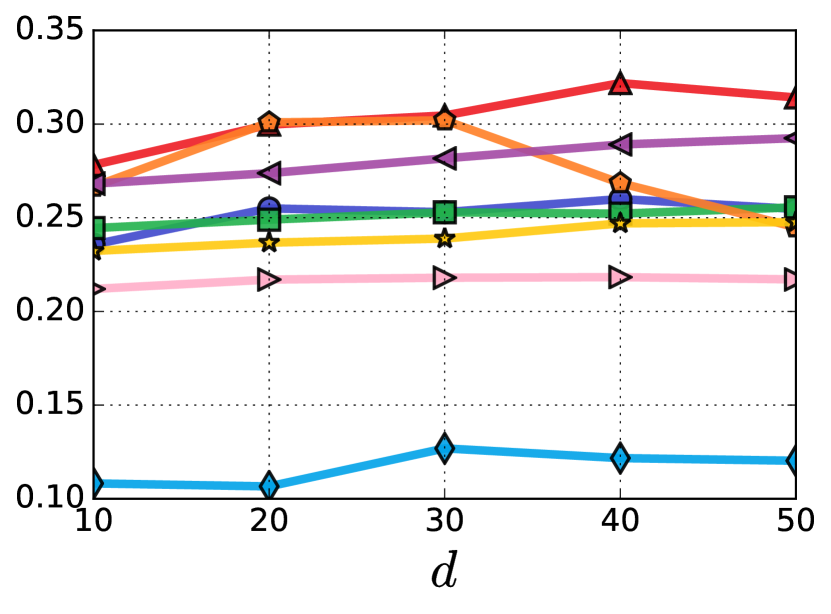
(a) Beauty

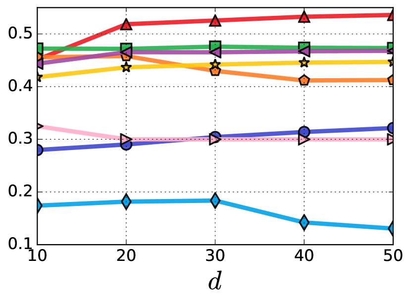
(b) Games

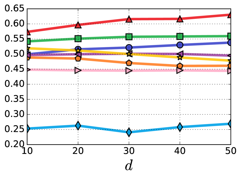
(c) Steam

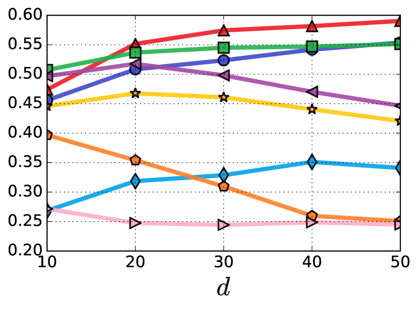
(d) ML-1M

Figure 2: Effect of the latent dimensionality $d$ on ranking performance (NDCG@10).

IV-F Ablation Study

Since there are many components in our architecture, we analyze their impacts via an ablation study (RQ2). Table IV shows the performance of our default method and its 8 variants on all four dataset (with $d=50$). We introduce the variants and analyze their effect respectively:

Table IV: Ablation analysis (NDCG@10) on four datasets. Performance better than the default version is boldfaced. ‘$\downarrow$’ indicates a severe performance drop (more than 10%).

Architecture	Beauty	Games	Steam	ML-1M
(0) Default	0.3142	0.5360	0.6306	0.5905
(1) Remove PE	0.3183	0.5301	0.6036	0.5772
(2) Unshared IE	0.2437$\downarrow$	0.4266$\downarrow$	0.4472$\downarrow$	0.4557$\downarrow$
(3) Remove RC	0.2591$\downarrow$	0.4303$\downarrow$	0.5693	0.5535
(4) Remove Dropout	0.2436$\downarrow$	0.4375$\downarrow$	0.5959	0.5801
(5) 0 Block ($b$=0)	0.2620$\downarrow$	0.4745$\downarrow$	0.5588$\downarrow$	0.4830$\downarrow$
(6) 1 Block ($b$=1)	0.3066	0.5408	0.6202	0.5653
(7) 3 Blocks ($b$=3)	0.3078	0.5312	0.6275	0.5931
(8) Multi-Head	0.3080	0.5311	0.6272	0.5885

• (1) Remove PE (Positional Embedding): Without the positional embedding ${\bf P}$, the attention weight on each item depends only on item embeddings. That is to say, the model makes recommendations based on users’ past actions, but their order doesn’t matter. This variant might be suitable for sparse datasets, where user sequences are typically short. This variant performs better then the default model on the sparsest dataset (Beauty), but worse on other denser datasets.

• (2) Unshared IE (Item Embedding): We find that using two item embeddings consistently impairs the performance, presumably due to overfitting.

• (3) Remove RC (Residual Connections): Without residual connections, we find that performance is significantly worse. Presumably this is because information in lower layers (e.g. the last item’s embedding and the output of the first block) can not be easily propagated to the final layer, and this information is highly useful for making recommendations, especially on sparse datasets.

• (4) Remove Dropout: Our results show that dropout can effectively regularize the model to achieve better test performance, especially on sparse datasets. The results also imply the overfitting problem is less severe on dense datasets.

• (5)-(7) Number of blocks: Not surprisingly, results are inferior with zero blocks, since the model would only depend on the last item. The variant with one block performs reasonably well, though using two blocks (the default model) still boosts performance especially on dense datasets, meaning that the hierarchical self-attention structure is helpful to learn more complex item transitions. Using three blocks achieves similar performance to the default model.

• (8) Multi-head: The authors of Transformer [3] found that it is useful to use ‘multi-head’ attention, which applies attention in $h$ subspaces (each a $d/h$-dimensional space). However, performance with two heads is consistently and slightly worse than single-head attention in our case. This might owe to the small $d$ in our problem ($d=512$ in Transformer), which is not suitable for decomposition into smaller subspaces.

IV-G Training Efficiency & Scalability

We evaluate two aspects of the training efficiency (RQ3) of our model: Training speed (time taken for one epoch of training) and convergence time (time taken to achieve satisfactory performance). We also examine the scalability of our model in terms of the maximum length $n$. All experiments are conducted with a single GTX-1080 Ti GPU.

Training Efficiency

Figure 3 demonstrates the efficiency of deep learning based methods with GPU acceleration. GRU4Rec is omitted due to its inferior performance. For fair comparison, there are two training options for Caser and GRU4Rec${}^{\text{+}}$: using complete training data or just the most recent 200 actions (as in SASRec). For computing speed, SASRec only spends 1.7 seconds on model updates for one epoch, which is over 11 times faster than Caser (19.1s/epoch) and 18 times faster than GRU4Rec${}^{\text{+}}$ (30.7s/epoch). We also see that SASRec converges to optimal performance within around 350 seconds on ML-1M while other models require much longer. We also find that using full data leads to better performance for Caser and GRU4Rec${}^{\text{+}}$.

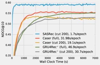
Figure 3: Training efficiency on ML-1M. SASRec is an order of magnitude faster than CNN/RNN-based recommendation methods in terms of training time per epoch and in total.

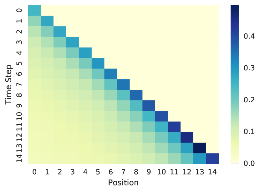
(a) Beauty, Layer 1

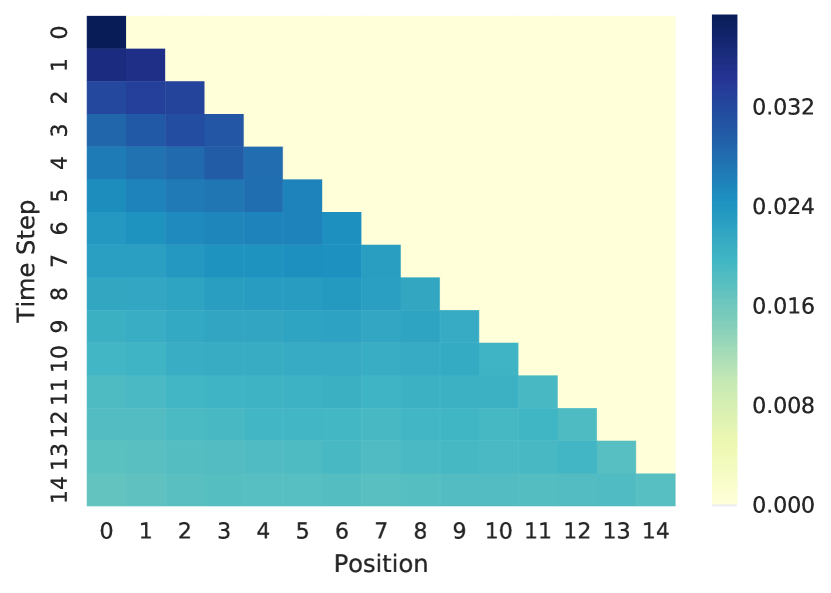
(b) ML-1M, Layer 1, w/o PE

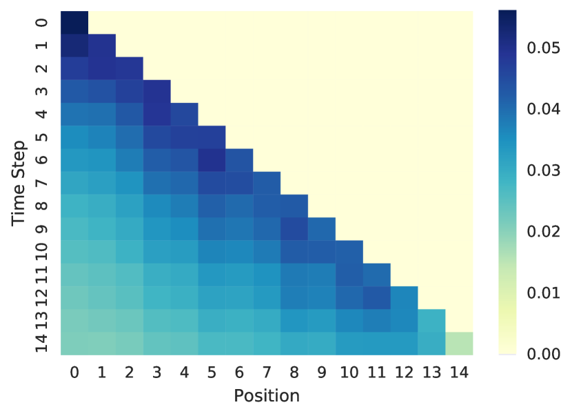
(c) ML-1M, Layer 1

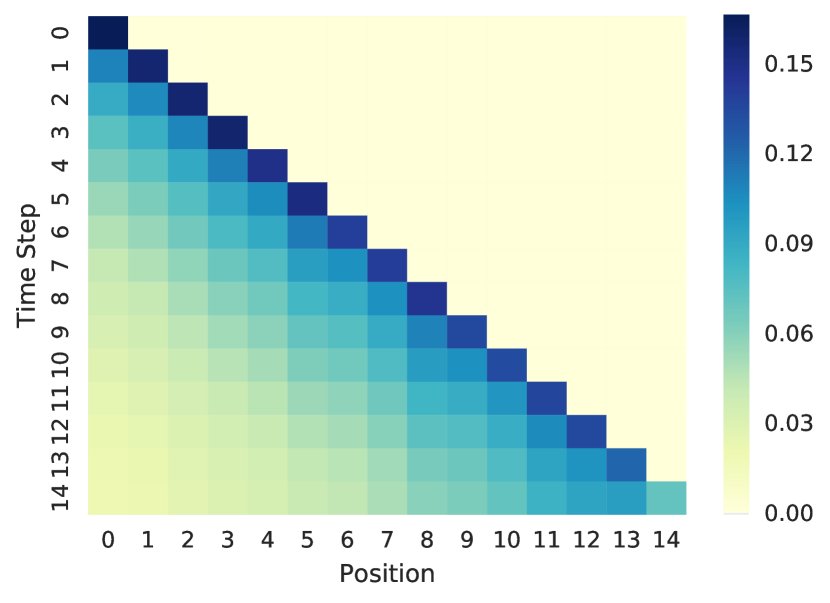
(d) ML-1M, Layer 2

Figure 4: Visualizations of average attention weights on positions at different time steps. For comparison, the heatmap of a first-order Markov chain based model would be a diagonal matrix.

Scalability

As with standard MF methods, SASRec scales linearly with the total number of users, items and actions. A potential scalability concern is the maximum length $n$, however the computation can be effectively parallelized with GPUs. Here we measure the training time and performance of SASRec with different $n$, empirically study its scalability, and analyze whether it can handle sequential recommendation in most cases. Table V shows the performance and efficiency of SASRec with various sequence lengths. Performance is better with larger $n$, up to around $n=500$ at which point performance saturates (possibly because 99.8% of actions have been covered). However, even with $n=600$, the model can be trained in 2,000 seconds, which is still faster than Caser and GRU4Rec${}^{\text{+}}$. Hence, our model can easily scale to user sequences up to a few hundred actions, which is suitable for typical review and purchase datasets. We plan to investigate approaches (discussed in Section III-F) for handling very long sequences in the future.

Table V: Scalability: performance and training time with different maximum length $n$ on ML-1M.

$n$	10	50	100	200	300	400	500	600
Time(s)	75	101	157	341	613	965	1406	1895
NDCG@10	0.480	0.557	0.571	0.587	0.593	0.594	0.596	0.595

IV-H Visualizing Attention Weights

Recall that at time step $t$, the self-attention mechanism in our model adaptively assigns weights on the first $t$ items depending on their position embeddings and item embeddings. To answer RQ4, we examine all training sequences and seek to reveal meaningful patterns by showing the average attention weights on positions as well as items.

Attention on Positions

Figure 4 shows four heatmaps of average attention weights on the last 15 positions at the last 15 time steps. Note that when we calculate the average weight, the denominator is the number of valid weights, so as to avoid the influence of padding items in short sequences.

We consider a few comparisons among the heatmaps:

• (a) vs. (c): This comparison indicates that the model tends to attend on more recent items on the sparse dataset Beauty, and less recent items for the dense dataset ML-1M. This is the key factor that allows our model to adaptively handle both sparse and dense datasets, whereas existing methods tend to focus on one end of the spectrum.

• (b) vs. (c): This comparison shows the effect of using positional embeddings (PE). Without them attention weights are essentially uniformly distributed over previous items, while the default model (c) is more sensitive in position as it is inclined to attend on recent items.

• (c) vs. (d): Since our model is hierarchical, this shows how attention varies across different blocks. Apparently, attention in high layers tends to focus on more recent positions. Presumably this is because the first self-attention block already considers all previous items, and the second block does not need to consider far away positions.

Overall, the visualizations show that the behavior of our self-attention mechanism is adaptive, position-aware, and hierarchical.

Attention Between Items

Showing attention weights between a few cherry-picked items might not be statistically meaningful. To perform a broader comparison, using MovieLens-1M, where each movie has several categories, we randomly select two disjoint sets where each set contains 200 movies from 4 categories: Science Fiction (Sci-Fi), Romance, Animation, and Horror. The first set is used for the query and the second set as the key. Figure 5 shows a heatmap of average attention weights between the two sets. We can see the heatmap is approximately a block diagonal matrix, meaning that the attention mechanism can identify similar items (e.g. items sharing a common category) and tends to assign larger weights between them (without being aware of categories in advance).

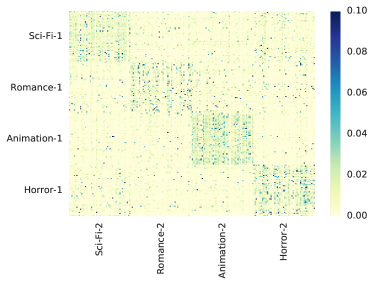
Figure 5: Visualization of average attention between movies from four categories. This shows our model can uncover items’ attributes, and assigns larger weights between similar items.

V Conclusion

In this work, we proposed a novel self-attention based sequential model SASRec for next item recommendation. SASRec models the entire user sequence (without any recurrent or convolutional operations), and adaptively considers consumed items for prediction. Extensive empirical results on both sparse and dense datasets show that our model outperforms state-of-the-art baselines, and is an order of magnitude faster than CNN/RNN based approaches. In the future, we plan to extend the model by incorporating rich context information (e.g. dwell time, action types, locations, devices, etc.), and to investigate approaches to handle very long sequences (e.g. clicks).

References

- [1] S. Rendle, C. Freudenthaler, and L. Schmidt-Thieme, “Factorizing personalized markov chains for next-basket recommendation,” in WWW, 2010.
- [2] B. Hidasi, A. Karatzoglou, L. Baltrunas, and D. Tikk, “Session-based recommendations with recurrent neural networks,” in ICLR, 2016.
- [3] A. Vaswani, N. Shazeer, N. Parmar, J. Uszkoreit, L. Jones, A. N. Gomez, L. Kaiser, and I. Polosukhin, “Attention is all you need,” in NIPS, 2017.
- [4] Y. Hu, Y. Koren, and C. Volinsky, “Collaborative filtering for implicit feedback datasets,” in ICDM, 2008.
- [5] S. Rendle, C. Freudenthaler, Z. Gantner, and L. Schmidt-Thieme, “BPR: bayesian personalized ranking from implicit feedback,” in UAI, 2009.
- [6] F. Ricci, L. Rokach, B. Shapira, and P. Kantor, Recommender systems handbook. Springer US, 2011.
- [7] Y. Koren and R. Bell, “Advances in collaborative filtering,” in Recommender Systems Handbook. Springer, 2011.
- [8] S. Kabbur, X. Ning, and G. Karypis, “Fism: factored item similarity models for top-n recommender systems,” in SIGKDD, 2013.
- [9] S. Zhang, L. Yao, and A. Sun, “Deep learning based recommender system: A survey and new perspectives,” arXiv, vol. abs/1707.07435, 2017.
- [10] S. Wang, Y. Wang, J. Tang, K. Shu, S. Ranganath, and H. Liu, “What your images reveal: Exploiting visual contents for point-of-interest recommendation,” in WWW, 2017.
- [11] W. Kang, C. Fang, Z. Wang, and J. McAuley, “Visually-aware fashion recommendation and design with generative image models,” in ICDM, 2017.
- [12] H. Wang, N. Wang, and D. Yeung, “Collaborative deep learning for recommender systems,” in SIGKDD, 2015.
- [13] D. H. Kim, C. Park, J. Oh, S. Lee, and H. Yu, “Convolutional matrix factorization for document context-aware recommendation,” in RecSys, 2016.
- [14] X. He, L. Liao, H. Zhang, L. Nie, X. Hu, and T. Chua, “Neural collaborative filtering,” in WWW, 2017.
- [15] S. Sedhain, A. K. Menon, S. Sanner, and L. Xie, “Autorec: Autoencoders meet collaborative filtering,” in WWW, 2015.
- [16] Y. Koren, “Collaborative filtering with temporal dynamics,” Communications of the ACM, 2010.
- [17] C. Wu, A. Ahmed, A. Beutel, A. J. Smola, and H. Jing, “Recurrent recommender networks,” in WSDM, 2017.
- [18] L. Xiong, X. Chen, T.-K. Huang, J. Schneider, and J. G. Carbonell, “Temporal collaborative filtering with bayesian probabilistic tensor factorization,” in SDM, 2010.
- [19] R. He, W. Kang, and J. McAuley, “Translation-based recommendation,” in RecSys, 2017.
- [20] R. He, C. Fang, Z. Wang, and J. McAuley, “Vista: A visually, socially, and temporally-aware model for artistic recommendation,” in RecSys, 2016.
- [21] R. He and J. McAuley, “Fusing similarity models with markov chains for sparse sequential recommendation,” in ICDM, 2016.
- [22] J. Tang and K. Wang, “Personalized top-n sequential recommendation via convolutional sequence embedding,” in WSDM, 2018.
- [23] H. Jing and A. J. Smola, “Neural survival recommender,” in WSDM, 2017.
- [24] Q. Liu, S. Wu, D. Wang, Z. Li, and L. Wang, “Context-aware sequential recommendation,” in ICDM, 2016.
- [25] A. Beutel, P. Covington, S. Jain, C. Xu, J. Li, V. Gatto, and E. H. Chi, “Latent cross: Making use of context in recurrent recommender systems,” in WSDM, 2018.
- [26] B. Hidasi and A. Karatzoglou, “Recurrent neural networks with top-k gains for session-based recommendations,” CoRR, vol. abs/1706.03847, 2017.
- [27] K. Xu, J. Ba, R. Kiros, K. Cho, A. C. Courville, R. Salakhutdinov, R. S. Zemel, and Y. Bengio, “Show, attend and tell: Neural image caption generation with visual attention,” in ICML, 2015.
- [28] D. Bahdanau, K. Cho, and Y. Bengio, “Neural machine translation by jointly learning to align and translate,” in ICLR, 2015.
- [29] J. Chen, H. Zhang, X. He, L. Nie, W. Liu, and T. Chua, “Attentive collaborative filtering: Multimedia recommendation with item- and component-level attention,” in SIGIR, 2017.
- [30] J. Xiao, H. Ye, X. He, H. Zhang, F. Wu, and T. Chua, “Attentional factorization machines: Learning the weight of feature interactions via attention networks,” in IJCAI, 2017.
- [31] S. Wang, L. Hu, L. Cao, X. Huang, D. Lian, and W. Liu, “Attention-based transactional context embedding for next-item recommendation,” in AAAI, 2018.
- [32] Y. Wu, M. Schuster, Z. Chen, Q. V. Le, M. Norouzi, W. Macherey, M. Krikun, Y. Cao, Q. Gao, K. Macherey et al., “Google’s neural machine translation system: Bridging the gap between human and machine translation,” arXiv preprint arXiv:1609.08144, 2016.
- [33] J. Zhou, Y. Cao, X. Wang, P. Li, and W. Xu, “Deep recurrent models with fast-forward connections for neural machine translation,” TACL, 2016.
- [34] M. D. Zeiler and R. Fergus, “Visualizing and understanding convolutional networks,” in ECCV, 2014.
- [35] K. He, X. Zhang, S. Ren, and J. Sun, “Deep residual learning for image recognition,” in CVPR, 2016.
- [36] L. J. Ba, R. Kiros, and G. E. Hinton, “Layer normalization,” CoRR, vol. abs/1607.06450, 2016.
- [37] S. Ioffe and C. Szegedy, “Batch normalization: Accelerating deep network training by reducing internal covariate shift,” in ICML, 2015.
- [38] N. Srivastava, G. E. Hinton, A. Krizhevsky, I. Sutskever, and R. Salakhutdinov, “Dropout: a simple way to prevent neural networks from overfitting,” JMLR, 2014.
- [39] D. Warde-Farley, I. J. Goodfellow, A. C. Courville, and Y. Bengio, “An empirical analysis of dropout in piecewise linear networks,” CoRR, vol. abs/1312.6197, 2013.
- [40] Y. Koren, R. Bell, and C. Volinsky, “Matrix factorization techniques for recommender systems,” Computer, 2009.
- [41] D. P. Kingma and J. Ba, “Adam: A method for stochastic optimization,” in ICLR, 2015.
- [42] D. Povey, H. Hadian, P. Ghahremani, K. Li, and S. Khudanpur, “A time-restricted self-attention layer for asr,” in ICASSP, 2018.
- [43] P. Wang, J. Guo, Y. Lan, J. Xu, S. Wan, and X. Cheng, “Learning hierarchical representation model for next basket recommendation,” in SIGIR, 2015.
- [44] S. Bai, J. Z. Kolter, and V. Koltun, “An empirical evaluation of generic convolutional and recurrent networks for sequence modeling,” CoRR, vol. abs/1803.01271, 2018.
- [45] S. Hochreiter, Y. Bengio, P. Frasconi, J. Schmidhuber et al., “Gradient flow in recurrent nets: the difficulty of learning long-term dependencies,” 2001.
- [46] J. J. McAuley, C. Targett, Q. Shi, and A. van den Hengel, “Image-based recommendations on styles and substitutes,” in SIGIR, 2015.
- [47] S. Feng, X. Li, Y. Zeng, G. Cong, Y. M. Chee, and Q. Yuan, “Personalized ranking metric embedding for next new poi recommendation,” in IJCAI, 2015.
- [48] Y. Koren, “Factorization meets the neighborhood: a multifaceted collaborative filtering model,” in SIGKDD, 2008.