Universal non-mean-field scaling in the density of state of amorphous solids

Abstract

Amorphous solids have excess soft modes in addition to the phonon modes described by the Debye theory. Recent numerical results show that if the phonon modes are carefully removed, the density of state of the excess soft modes exhibit universal quartic scaling, independent of the interaction potential, preparation protocol, and spatial dimensions. We hereby provide a theoretical framework to describe this universal scaling behavior. For this purpose, we extend the mean-field theory to include the effects of finite dimensional fluctuation. Based on a semi-phenomenological argument, we show that mean-field quadratic scaling is replaced by the quartic scaling in finite dimensions. Furthermore, we apply our formalism to explain the pressure and protocol dependence of the excess soft modes.

Introduction.– The vibrational density of state $D(\omega)$ of amorphous solid differs dramatically from that of crystals. The low-frequency modes of crystals are phonons that follow the Debye law $D(\omega)\sim\omega^{d-1}$, where $d$ denotes the spatial dimensions Kittel et al. (1996). On the contrary, $D(\omega)/\omega^{d-1}$ of amorphous solids exhibit a sharp peak at the characteristic frequency $\omega=\omega_{\rm BP}$, which is referred to as the Boson peak (BP). This behavior suggests the existence of excess soft modes (ESMs) beyond that predicted by the Debye law Anderson et al. (2012); Buchenau et al. (1984); Malinovsky and Sokolov (1986). For $\omega<\omega_{\rm BP}$, the ESMs are spatially localized Taraskin and Elliott (1999); Laird and Schober (1991); Mazzacurati et al. (1996); Chen et al. (2010); Liu et al. (2011). These localized modes play a central role in controlling the various low-temperature properties of amorphous solids, such as the specific heat, thermal conduction, and sound attenuation Anderson et al. (2012); Zeller and Pohl (1971); Anderson et al. (1972); Phillips (1972). Furthermore, recent numerical studies have established that the ESMs facilitate the structural relaxation of supercooled liquids at finite temperatures Widmer-Cooper and Harrowell (2006); Widmer-Cooper et al. (2008); Lerner and Bouchbinder (2018), and the local rearrangement of sheared amorphous solids at low temperature Xu et al. (2010); Manning and Liu (2011); Ding et al. (2014); Ji et al. (2018); Kapteijns et al. (2018a).

The detailed statistical properties of ESMs have been only recently investigated via numerical simulations. The ESMs can be separated from the background phonon modes by using a small size system Lerner et al. (2016), observing the participation ratio Mizuno et al. (2017), or introducing impurities Baity-Jesi et al. (2015); Angelani et al. (2018). Remarkably, after successfully removal of the phonons, the ESMs follow the universal quartic law $D(\omega)=A_{4}\omega^{4}$ for $\omega\ll\omega_{\rm BP}$, independent of the interaction potentials, preparation protocols and dimensions Lerner et al. (2016); Wang et al. (2018); Kapteijns et al. (2018b). Considering the relationship with other physical quantities, it is important to gain an understanding the mechanism that yields the $D(\omega)=A_{4}\omega^{4}$ law and controls the prefactor $A_{4}$.

The $d$ independence of the quartic law motivates us to apply mean-field theory to understand this scaling behavior. The replica theory is now one of the most mature mean-field theories of amorphous solids Castellani and Cavagna (2005); Parisi and Zamponi (2010); Biroli and Bouchaud (2012); Charbonneau et al. (2017). In particular, near the (un) jamming transition point at which the system loses rigidity O’hern et al. (2003); Liu et al. (2011), the theory predicts the exact critical exponents of the contact number and shear modulus DeGiuli et al. (2014); Charbonneau et al. (2017). Furthermore, the theoretical result of $D(\omega)$ agrees very well with the numerical results for $\omega>\omega_{\rm BP}$ in $d=2$ and $3$ DeGiuli et al. (2014); Franz et al. (2017). The replica theory predicts that amorphous solids near the jamming transition point are in the Gardner phase Charbonneau et al. (2017); Biroli and Urbani (2018), which has been originally investigated in a class of mean-field spin glasses Gardner (1985); Gross et al. (1985). In the Gardner phase, the density of state has the gapless excitation $D(\omega)\sim\omega^{2}$ for $\omega<\omega_{\rm BP}$ Franz et al. (2017). However, the numerical results indicate that $D(\omega)\sim\omega^{2}$ scaling is observed only near $\omega\sim\omega_{\rm BP}$, and it is replaced by $D(\omega)\sim A_{4}\omega^{4}$ for $\omega\ll\omega_{\rm BP}$ Mizuno et al. (2017).

The mean-field replica calculation predicts another source of the singularity that creates the ESMs, in addition to the trivial phonon modes. This singularity is related to the quenching rate, or from a theoretical perspective, the initial temperature $T_{\rm ini}$ of the equilibrium supercooled liquid before quenching to produce glass. When $T_{\rm ini}$ is sufficiently low, the supercooled liquid becomes highly viscous because of the complex structure of the free-energy landscape containing multiple minima Goldstein (1969). After quenching, the system falls to one of the minima. The minima become gradually unstable with an increase in temperature and eventually disappear above the so-called mode coupling transition point $T_{\rm mct}$ Castellani and Cavagna (2005); Biroli and Bouchaud (2012). This instability affects the vibrational properties of the zero-temperature amorphous solids and creates ESMs Parisi (2002). This view seems to be consistent with the numerical result that the excess soft modes close to $\omega\sim\omega_{\rm BP}$ are indeed enhanced for samples quenched from higher temperatures Grigera et al. (2003). However, the mean-field prediction, $D(\omega)\sim\omega^{2}$ for $\omega<\omega_{\rm BP}$, is again inconsistent with the numerical result where $D(\omega)\sim A_{4}\omega^{4}$ scaling is robustly observed irrespective of $T_{\rm ini}$ Wang et al. (2018).

In this Letter, we reconcile the aforementioned discrepancies between the mean-field replica theory and the numerical results in finite $d$ for small $\omega$ by introducing the effect of the finite $d$ fluctuation to the mean-field density of state in a semi-phenomenological way. We initially construct a theory to describe the asymptotic behavior of $D(\omega)$ in high $d$ and show that the quartic law naturally arises as a consequence of finite $d$ fluctuation. Next, motivated by the $d$ independence of the $D(\omega)\sim A_{4}\omega^{4}$ scaling Kapteijns et al. (2018b), we apply our formalism to explain the numerical results in $d=3$. We show that our theory well reproduces the correct scaling behavior of the prefactor $A_{4}$ near jamming and the $T_{\rm ini}$ dependence of $A_{4}$ for $T_{\rm ini}\sim T_{\rm mct}$.

Effect of the finite dimensional fluctuation.– Recent numerical results confirm that the small $\omega$ behavior of the ESMs, $D(\omega)\sim A_{4}\omega^{4}$, does not depend on the spatial dimensions $d$ Kapteijns et al. (2018b). Despite this seemingly mean-field like behavior, mean-field theory fails to reproduce this quartic law. We first review the discrepancy between the mean-field and numerical results in high but finite $d$ and then discuss an approach for solving this problem.

In the mean-field replica theory, amorphous solids are modeled by fully connected models, which are considered to correspond to the $d\to$ limit of the system. The fully connected models have the universal form of the eigenvalue distribution function for small $\lambda$, $\rho(\lambda)\sim\sqrt{\lambda-\varepsilon}$ sm , where $\varepsilon$ is proportional to the distance to the instability point. The mean-field theory predicts that if an amorphous solid is quenched from high temperature or located near the jamming transition point, the system becomes marginally stable $\varepsilon=0$ Franz et al. (2015); Cugliandolo and Kurchan (1993), thus we have

$$\rho_{\rm MF}(\lambda)\sim\sqrt{\lambda}\theta(\lambda),$$ (1)

where $\theta(x)$ denotes the Heaviside step function. The density of state $D(\omega)$ is obtained by changing the variable as $\omega=\sqrt{\lambda}$, which leads to $D(\omega)=2\omega\rho_{\rm MF}(\lambda=\omega^{2})\sim\omega^{2}$ for small $\omega$. In Fig. 1, we compare the mean-field prediction with the numerical result in $d=4$ to $7$. For $\omega>\omega_{0}\approx 0.12$, the numerical result converges to the mean-field prediction $D(\omega)\sim\omega^{2}$ for an increase of $d$. On the contrary, for $\omega<\omega_{0}$, the data systematically deviate from the mean-field prediction and are well fitted by $D(\omega)\sim\omega^{4}$, as already confirmed by previous numerical simulations in $d=3$ and $4$ Lerner et al. (2016); Kapteijns et al. (2018b). For very small $\omega$, the numerical results are scattered around $10^{-4}$, presumably owing to the finite size effect or the lack of statistics (not shown). We are aware that the size of the current system $N=8192$ is not large enough to observe the effects of phonons Kapteijns et al. (2018b). Nevertheless, we believe that these effects can be negligible in $d>5$ because the contribution of the ESMs, $D(\omega)\sim\omega^{4}$, overwhelms the phonon contribution, $D(\omega)\sim\omega^{d-1}$.

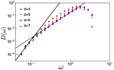
Figure 1: Density of state $D(\omega)$ of harmonic spheres far from the jamming $\Delta\varphi/\varphi_{J}=1.4$ generated by the fast quench in $d=4$ to $7$. The system size is $N=8192$. Markers denote the numerical result, while the dashed and solid lines denote the theoretical predictions, $D(\omega)\sim\omega^{2}$ and $\omega^{4}$, respectively. Data are reproduced from Ref. Charbonneau et al. (2016).

To clarify the reason for the above discrepancy between the mean-field and numerical result for finite $d$, we decompose the $i$-th eigenvalue $\lambda_{i}$ into the following two parts:

$$\lambda_{i}=\lambda_{i}^{\rm MF}+\varepsilon_{i},$$ (2)

where $\lambda_{i}^{\rm MF}$ follows the mean-field result Eq. (1) and $\varepsilon_{i}$ represents the finite $d$ fluctuation. Then, the distribution function of $\lambda_{i}$ is

$$\rho(\lambda)=\left\langle\delta(\lambda-\lambda_{i})\right\rangle=\int_{0}^{\infty}d\varepsilon\mathcal{P}_{\lambda}(\varepsilon)\rho_{\rm MF}(\lambda-\varepsilon),$$ (3)

where the lower bound of the integral arises from the stability condition, $\rho(\lambda)=0$ for $\lambda<0$, and we introduced the conditional probability distribution:

$$\mathcal{P}_{\lambda}(\varepsilon)=\frac{\left\langle\delta(\varepsilon-\varepsilon_{i})\delta(\lambda-\varepsilon-\lambda_{i}^{\rm MF})\right\rangle}{\left\langle\delta(\lambda-\varepsilon-\lambda_{i}^{\rm MF})\right\rangle}.$$ (4)

In the $d\to\infty$ limit, the system can be identified with the fully connected model and thus $\mathcal{P}_{\lambda}(\varepsilon)=\delta(\varepsilon)$ to recover the mean-field result. For high but finite $d$, $\mathcal{P}_{\lambda}(\varepsilon)$ is expected to have a narrow distribution close to $\varepsilon=0$. Thus, we set a small cutoff $\Delta$ and assume that $\mathcal{P}_{\lambda}(\varepsilon)=O(1)$ for $\varepsilon\ll\Delta$ and $\mathcal{P}_{\lambda}(\varepsilon)\sim 0$ for $\varepsilon\gg\Delta$. Using Eqs. (1) and (3), we obtain the following for $\lambda\ll\Delta$:

$$\rho(\lambda) \sim\mathcal{P}_{0}(0)\int_{0}^{\lambda}d\varepsilon\sqrt{\lambda-\varepsilon}\sim\mathcal{P}_{0}(0)\lambda^{3/2},$$ (5)

leading to $D(\omega)\sim\omega^{4}$. Thus, the mean-field result is replaced by the quartic scaling unless the finite dimensional fluctuation is negligible, i.e., $\mathcal{P}_{\lambda}(\varepsilon)=\delta(\varepsilon)$. A similar calculation leads to $\rho(\lambda)\sim\rho_{\rm MF}(\lambda)$ for $\lambda\gg\Delta$, meaning that $D(\omega)\sim\omega^{2}$ for $\omega\gg\omega_{0}\equiv\sqrt{\Delta}$. Herewith we recover the numerical results for high $d$ in Fig. 1.

The $D(\omega)\sim\omega^{4}$ law is also obtained by a seemingly different approach: the so-called soft-potential model where the localized modes are modeled by the collection of anharmonic oscillators of different stiffnesses Ilyin et al. (1987); Buchenau et al. (1992); Gurarie and Chalker (2002). The advantage of our approach over that of the soft-potential model is that we can consider how the control parameters and preparation protocols affect the prefactor $A_{4}$ by relying on the mature replica theory, as shown in the following sections.

In general, it is impossible to calculate $\mathcal{P}_{\lambda}(\varepsilon)$ exactly for finite $d$. To simplify the treatment, we neglect the $\lambda$ dependence $\mathcal{P}_{\lambda}(\varepsilon)\approx\mathcal{P}(\varepsilon)$, which is tantamount to neglecting the higher order terms of $\lambda$ and can be justified for small $\lambda$. Then, Eq. (3) reduces to

$$\rho(\lambda)=\int_{0}^{\infty}d\varepsilon\mathcal{P}(\varepsilon)\rho_{\rm MF}(\lambda-\varepsilon).$$ (6)

From the normalization conditions of $\rho(\lambda)$ and $\rho_{\rm MF}(\lambda)$, it can be shown that $\int_{0}^{\infty}d\varepsilon\mathcal{P}(\varepsilon)=1$, suggesting that $\mathcal{P}(\varepsilon)$ can be considered as the distribution function of the distance to the instability point $\varepsilon$. The fluctuation of $\varepsilon$ is a consequence of the spatial heterogeneity of amorphous solids, which are not considered in the fully connected mean-field models Xia and Wolynes (2000); Franz et al. (2011); Biroli et al. (2014). The width $\Delta$ of the distribution $\mathcal{P}(\varepsilon)$ decreases with an increase of $d$ as the system approaches the fully connected model. From the central limit theorem, we expect $\Delta\sim d^{-1/2}$ and the crossover frequency decreases as $\omega_{0}\sim d^{-1/4}$. However, it is difficult to detect such weak $d$ dependence from the current numerical result in Fig. 1. Further numerical investigations are necessary to confirm the $d$ dependence of $\Delta$.

Hereafter, we use a similar argument as that used to derive Eq. (6) to analyze the numerical results in $d=3$. Given that the proposed theory does not taken into account the phonon mode, the phonon contribution should be removed from the numerical results as in Refs. Lerner et al. (2016); Mizuno et al. (2017); Angelani et al. (2018), before comparing with the theoretical prediction.

Pressure dependence near jamming.– Here we investigate the pressure $p$ dependence of $D(\omega)$ near the jamming. For this purpose, we investigate the negative perceptron model, a mean-field model of the jamming transition that belongs to the same universality class of hard/harmonic spheres in the $d\to\infty$ limit Franz and Parisi (2016); Franz et al. (2017). The simplicity of the model allows for analytical calculation of the eigenvalue distribution function Franz et al. (2015). Near jamming, the model predicts for $\lambda\ll 1$ Franz et al. (2015)

$$\rho_{\rm MF}(\lambda)\sim\frac{\sqrt{\lambda}}{\lambda+\omega_{*}^{2}}\theta(\lambda),$$ (7)

where $\omega_{*}=c\sqrt{p}$, and $c$ is a constant. Essentially the same result as Eq. (7) is obtained by the effective medium theory, except for the trivial Debye modes DeGiuli et al. (2014). The gapless form of Eq. (7) is a consequence of the Gardner transition Franz et al. (2017), which is the continuous replica symmetric breaking transition originally discovered in the mean-field spin glasses Gardner (1985); Gross et al. (1985). From Eq. (7), the scaling behavior of $D(\omega)$ near jamming ($p\ll 1$) is given as:

$$D(\omega)\sim\begin{cases}{\rm constant}&(\omega\gtrsim\omega_{*}),\\ (\omega/\omega_{*})^{2}&(\omega\ll\omega_{*}).\end{cases}$$ (8)

However, this is inconsistent with the numerical result in $d=3$. The numerical result shows that if one carefully removes the phonon modes by using the participation ratio, one obtains Mizuno et al. (2017)

$$D(\omega)\sim\begin{cases}{\rm constant}&(\omega\gtrsim\omega_{*}),\\ (\omega/\omega_{*})^{2}&(\omega_{0}\ll\omega\ll\omega_{*}),\\ (\omega/\omega_{*})^{4}&(\omega\ll\omega_{0}),\end{cases}$$ (9)

where $\omega_{0}\propto\sqrt{p}$ but the proportionality constant is much smaller than that of $\omega_{*}$.

One of the reasons for the discrepancy between the mean-field theory and the numerical results is the absence of the marginal stability for finite $d$. The numerical results show that the mean distance to the instability point has a finite value Lerner et al. (2014); DeGiuli et al. (2014),

$$\left\langle\varepsilon\right\rangle=p\Delta_{\rm G},$$ (10)

where $\Delta_{\rm G}$ is a small positive constant. As in Eq. (6), we introduce the fluctuation of $\varepsilon$ and assume that the mean value of the eigenvalue distribution function can be written as follows:

$$\rho(\lambda)=\int_{0}^{\infty}d\varepsilon\mathcal{P}(\varepsilon)\rho_{\rm MF}(\lambda-\varepsilon).$$ (11)

From Eq. (10), $\mathcal{P}(\varepsilon)$ should be $\mathcal{P}(\varepsilon)=O(p^{-1}\Delta_{\rm G}^{-1})$ for $\varepsilon<p\Delta_{\rm G}$ and quickly decreases for $\varepsilon>p\Delta_{\rm G}$. Repeating a similar argument in Eq. (5), we obtain for $\lambda\ll p\Delta_{\rm G}$

$$\rho(\lambda) \sim c^{2}\Delta_{\rm G}^{-1}\omega_{*}^{-4}\lambda^{3/2},$$ (12)

which leads to $D(\omega)\sim c^{2}\Delta_{\rm G}^{-1}(\omega/\omega_{*})^{4}$. This scaling smoothly connects to the mean-field scaling Eq. (8) at $\omega\sim\omega_{0}\equiv\sqrt{p\Delta_{\rm G}}$. Thus, we reproduced the numerical result, Eq. (9). Finally, for concreteness, in Fig. 2, we show $D(\omega)$ calculated by Eq. (11) assuming $\mathcal{P}(\varepsilon)=(p\Delta_{\rm G})^{-1}e^{-(p\Delta_{\rm G})^{-1}\varepsilon}$, $\Delta_{\rm G}=10^{-4}$, and $c=1$. If one rescales $\omega$ by $\omega_{*}$, the data for different $p$ are collapsed on a single curve as expected from Eq. (9).

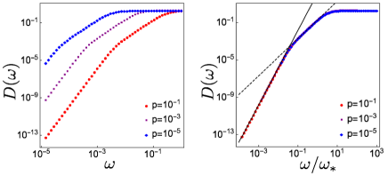
Figure 2: The density of state $D(\omega)$: (left) The results for $p=10^{-1}$, $10^{-3}$ and $10^{-5}$. (right) The scaling plot for the same data. The dashed and solid lines indicate $D(\omega)\sim\omega^{2}$ and $D(\omega)\sim\omega^{4}$, respectively.

Initial temperature dependence.– Here, we discuss the influence of $T_{\rm ini}$ on the vibrational properties of amorphous solids at zero temperature. For this purpose, we start from the $p$-spin spherical model (PSM), which is a prototypical mean-field model for glass transition to discuss the connection between the glassy slow dynamics and complex free energy landscape Castellani and Cavagna (2005); Biroli and Bouchaud (2012). The replica calculation of the PSM shows that there are many metastable states on the free energy landscape below $T_{\rm mct}$. After quenching, the system falls to one of the minima. On the minima, the eigenvalue distribution function of the PSM follows the Wigner semicircle law Kurchan and Laloux (1996); Biroli and Bouchaud (2012). For $\lambda\ll 1$ and $T_{\rm ini}\approx T_{\rm mct}$, this can be written as

$$\rho_{\rm MF}(\lambda)\sim\sqrt{\lambda-\lambda_{\rm min}}\theta(\lambda-\lambda_{\rm min}),$$ (13)

where $\lambda_{\rm min}=c(T_{\rm mct}-T_{\rm ini})$ for $T_{\rm ini}<T_{\rm mct}$, and $\lambda_{\rm min}=0$ for $T_{\rm ini}\geq T_{\rm mct}$ Cugliandolo and Kurchan (1993). $c$ is a positive constant. Repeating a similar argument that used to derive Eq. (6), we obtain

$$\rho(\lambda)=\int_{-\lambda_{\rm min}}^{\infty}d\varepsilon\mathcal{P}(\varepsilon)\rho_{\rm MF}(\lambda-\varepsilon),$$ (14)

where the lower bound of the integral is followed by the stability condition, $\rho(\lambda)=0$ for $\lambda<0$. As mentioned, $\mathcal{P}(\varepsilon)$ is expected to have a narrow distribution close to $\varepsilon=0$. To express this distribution, we assume

$$\mathcal{P}(\varepsilon) \sim\Delta_{\rm mct}^{-1}\exp\left[-\left|\frac{\varepsilon}{\Delta_{\rm mct}}\right|^{\alpha}\right],$$ (15)

where $\Delta_{\rm mct}$ and $\alpha$ are constants. Then, the eigenvalue distribution for small $\lambda$ is calculated as

$$\rho(\lambda) \sim\mathcal{P}(-\lambda_{\rm min})\int_{-\lambda_{\rm min}}^{\lambda-\lambda_{\rm min}}d\varepsilon\sqrt{\lambda-\lambda_{\rm min}-\varepsilon}$$

$$\sim\mathcal{P}(-\lambda_{\rm min})\lambda^{3/2},$$ (16)

leading to

$$D(\omega)=A_{4}\omega^{4},$$ (17)

where the prefactor is given as:

$$A_{4} =\begin{cases}A&(T_{\rm ini}\geq T_{\rm mct})\\ A\exp\left[-\left(\frac{T_{\rm mct}-T_{\rm ini}}{\hat{\Delta}_{\rm mct}}\right)^{\alpha}\right]&(T_{\rm ini}<T_{\rm mct})\end{cases}.$$ (18)

$A$ is a constant and $\hat{\Delta}_{\rm mct}=\Delta_{\rm mct}/c$. The preceding equation shows that $A_{4}$ rapidly decreases for $T_{\rm mct}-T_{\rm ini}>\hat{\Delta}_{\rm mct}$.

Figure 3: The $T_{\rm ini}$ dependence of $A_{4}$ of soft-spheres in $d=3$. The circles and squares denote the numerical results of the system sizes $N=96000$ and $192000$, respectively. The solid line denotes the theoretical prediction, where $A=0.047$, $T_{\rm mct}=0.108$, $\hat{\Delta}_{\rm mct}=0.021$, and $\alpha=1.22$. (Inset): The same figure in the semi-log scale. Data are reproduced from Ref. Wang et al. (2018).

In Fig. 3, we compare our prediction with the numerical results of an amorphous solid in $d=3$. An excellent agreement is realized which proves the validity of our theory.

Conclusions and discussions.– In summary, we discussed the process by which finite dimensional fluctuation alters the mean-field scaling $D(\omega)\sim\omega^{2}$ of amorphous solids. Our theory successfully captures quartic scaling, $D(\omega)\sim A_{4}\omega^{4}$, reported in previous numerical simulations. We applied the theory to describe the pressure $p$ and initial temperature $T_{\rm ini}$ dependence of the prefactor $A_{4}$. In both cases, the theoretical results are in good agreement with the previous numerical results. It should be noted that the argument in Eq. (5) does not depend on the precise form of $\mathcal{P}_{\lambda}(\varepsilon)$. If $\mathcal{P}_{\lambda}(\varepsilon)$ is finite and continuous at $\varepsilon=0$ and $\lambda=0$, one always obtains the quartic scaling for small $\omega$. This may explain the robustness of the quartic scaling against the different interaction potentials, preparation protocol, and dimensions Kapteijns et al. (2018b); Wang et al. (2018); Lerner et al. (2016); Mizuno et al. (2017); Shimada et al. (2018); Wang et al. (2018).

In this Letter, we proposed two singularities to yield the quartic scaling: singularities related to the Gardner and MCT transitions. Near the jamming transition point ($p\ll 1$), one can conclude that the Gardner transition plays the dominant role in generating quartic scaling considering the numerical and experimental evidence for the Gardner transition Berthier et al. (2016); Jin and Yoshino (2017); Seguin and Dauchot (2016) and the consistency between the mean-field and numerical results Charbonneau et al. (2014, 2017). However, this scenario may not hold apart from jamming where amorphous solids do not show the strong signature of the Gardner transition Scalliet et al. (2017); Seoane et al. (2018). In this region, the MCT transition would be the main cause of the quartic scaling. For the intermediate value of $p$, the situation is more complex and further investigations are needed to determine which singularity plays the dominant role.

If $\mathcal{P}_{\lambda}(\varepsilon)$ is not finite at $\varepsilon=0$ and $\lambda=0$, the $D(\omega)\sim\omega^{4}$ law can be replaced. For instance, if $\mathcal{P}_{\lambda}(\varepsilon)\sim A\varepsilon^{-\alpha}$ for small $\varepsilon$ and $\lambda$, a similar calculation as that used in Eq. (5) leads to $\rho(\lambda)\sim A\lambda^{3/2-\alpha}$. This implies that $D(\omega)\sim A\omega^{4-2\alpha}$. Interestingly, for amorphous solids prepared by instantaneous quenching without inertia, Lerner and Bouchbinder Lerner and Bouchbinder (2017) observed $D(\omega)\sim\omega^{\beta}$ with $\beta<4$ suggesting that $\alpha>0$. Also, some spring models for amorphous solids on the scale-free network Stanifer et al. (2018) and random graph Benetti et al. (2018) show that $\beta$ can change depending on the spatial dimensions and distribution of the coordination number. Further investigations are required to identify what physical mechanisms control $\alpha$ and $\beta$.

Appendix A Supplemental information for “Universal non-mean-field scaling in the density of state of amorphous solids”

Here we briefly explain the scaling behavior of the mean-field eigenvalue distribution near the minimal eigenvalue. For more complete and rigorous derivations, see for instance Refs. Edwards and Jones (1976); Livan et al. (2018). We consider a Hessian $H_{ij},\ i,j=1,\cdots,N$ of a fully connected model. The eigenvalue distribution function is obtained by using the Edwards and Jones formula Edwards and Jones (1976):

$$\rho(\lambda) =\frac{1}{N}\sum_{i=1}^{N}\delta(\lambda-\lambda_{i})$$

$$=\left|\frac{2}{\pi N}{\rm Im}\left[\frac{\partial}{\partial\lambda}\log Z(\lambda)\right]\right|,$$ (19)

where

$$Z(\lambda) =\int d\bm{u}\exp\left[-\frac{1}{2}\bm{u}\cdot\left(H-\lambda I\right)\bm{u}\right].$$ (20)

Introducing the new variable $q\equiv\bm{u}\cdot\bm{u}/N$ and using the saddle point method, $Z(\lambda)$ is calculated as

$$\log Z(\lambda)\approx N\left(\lambda\frac{q}{2}+G(q)\right),$$ (21)

where

$$G(q)=\frac{1}{N}\log\int d\bm{u}\delta(\bm{u}\cdot\bm{u}-Nq)e^{-\frac{1}{2}\bm{u}\cdot H\cdot\bm{u}}.$$ (22)

For fully connected models, one can directly calculate this quantity by using the replica method. However, the detailed functional form is not necessary for our purpose. The saddle point value of $q$ is determined by

$$\lambda=-2G^{\prime}(q).$$ (23)

Substituting Eq. (21) into Eq. (19), we have a simple result:

$$\rho(\lambda)=\left|\frac{1}{\pi}{\rm Im}[q(\lambda)]\right|.$$ (24)

$\rho(\lambda)$ would have a small value near the edge of the distribution. Eq. (24) implies that ${\rm Im}[q(\lambda)]$ is also small near that point. We expand the real and imaginary parts of Eq. (23) for ${\rm Im}[q]$:

$$\lambda=-2G^{\prime}({\rm Re}[q(\lambda)])+{\rm Im}[q(\lambda)]^{2}G^{\prime\prime\prime}({\rm Re}[q(\lambda)])+\cdots,$$

$$0={\rm Im}[q(\lambda)]G^{\prime\prime}({\rm Re}[q(\lambda)])+\cdots.$$ (25)

Then, ${\rm Im}[q(\lambda)]$ is calculated as

$${\rm Im}[q(\lambda)] \sim\sqrt{\frac{\lambda+2G^{\prime}({\rm Re}[q])}{G^{\prime\prime\prime}({\rm Re}[q])}}\sim\sqrt{\lambda-\varepsilon},$$ (26)

where $\varepsilon=-2G^{\prime}({\rm Re}[q])$ and ${\rm Re}[q]$ is determined by $G^{\prime\prime}({\rm Re}[q])=0$. From Eqs. (24) and (26), one can see that $\rho(\lambda)$ shows the square root singularity near the minimal eigenvalue $\rho(\lambda)\sim\sqrt{\lambda-\varepsilon}$.