A general weak and strong error analysis of the recursive quantization with an application to jump diffusions

Abstract

Observing that the recent developments of the recursive (product) quantization method induces a family of Markov chains which includes all standard discretization schemes of diffusions processes, we propose to compute a general error bound induced by the recursive quantization schemes using this generic markovian structure. Furthermore, we compute a marginal weak error for the recursive quantization. We also extend the recursive quantization method to the Euler scheme associated to diffusion processes with jumps, which still have this markovian structure, and we say how to compute the recursive quantization and the associated weights and transition weights.

1 Introduction

The $L^{r}$-optimal quantization problem for a random vector $X:(\Omega,\mathcal{A},\mathbb{P})\longrightarrow(\mathbb{R}^{d},|\cdot|)$ at level $N$ consists on finding the best (w.r.t. the $L^{r}$-mean error) approximation of $X$ by a Borel function taking at most $N$ values. Assuming that $X\in L^{r}_{\mathbb{R}^{d}}(\mathbb{P})$, this boils down to solve the following minimization problem

$$e_{N,r}(X)=\inf{\{\|X-\hat{X}^{\Gamma}\|_{r},\ \Gamma\subset\mathbb{R}^{d},\ |\Gamma|\leq N\}}=\inf_{\begin{subarray}{c}\Gamma\subset\mathbb{R}^{d}\\ |\Gamma|\leq N\end{subarray}}\left(\int_{\mathbb{R}^{d}}{\rm dist}(x,\Gamma)^{r}d\mathbb{P}_{X}(x)\right)^{1/r}$$ (1)

where $|\Gamma|$ denotes the cardinality of the set (or grid) $\Gamma$ and $\|X\|_{r}=\big{[}\mathds{E}\,|X|^{r}\big{]}^{1/r}$ ($|\cdot|$ may be a priori any norm on $\mathbb{R}^{d}$), $\mathds{P}_{X}$ denotes the distribution of $X$. The quantity $\widehat{X}^{\Gamma}$ is called a Voronoi or nearest neighbour quantization of $X$ on a grid $\Gamma=\{x_{1},\ldots,x_{N}\}\subset\mathbb{R}^{d}$, and is defined as $\hat{X}^{\Gamma}=\sum_{i=1}^{N}x_{i}\mathds{1}_{\{X\in C_{i}(\Gamma)\}}$, where $C_{i}(\Gamma)_{i=1,\cdots,N}$ is a Borel partition of $\mathbb{R}^{d}$ (called a Voronoi partition of $\mathbb{R}^{d}$) satisfying for every $i\in\{1,\cdots,N\}$,  $C_{i}(\Gamma)\subset\big{\{}x\in\mathbb{R}^{d}:|x-x_{i}|=\min_{j=1,\cdots,N}|x-x_{j}|\big{\}}$. The infimum in (1) is in fact a minimum i.e., for any level $N\!\in\mathbb{N}$, there exists an optimal quantization grid $\Gamma^{(N)}$ solution to the above mimimization problem. For more insight on optimal quantization theory, we refer to [5] or, for more applied topics, to [10].

The quantization error $e_{N,r}(X)$ decreases to zero at the rate $N^{-1/d}$ as the grid size $N$ goes to infinity (this results is known as the Zador Theorem, see e.g. [5]). There is also a non-asymptotic upper bound for optimal quantizers called Pierce Lemma and stated as follows in the quadratic case (see [5, 7]): Let $p>2$. There exists a universal constant $C_{d,p,|\cdot|}$ such that for every random vector $X:(\Omega,{\cal A},\mathbb{P})\rightarrow(\mathbb{R}^{d},|\cdot|)$,

$$\inf_{|\Gamma|\leq N}\|X-\widehat{X}^{\Gamma}\|_{{}_{2}}\leq C_{d,p,|\cdot|}\,\sigma_{p}(X)N^{-\frac{1}{d}}$$ (2)

where

$$\sigma_{p}(X)=\inf_{\zeta\in\mathbb{R}^{d}}\|X-\zeta\|_{{}_{p}}\leq+\infty.$$

It will be briefly revisited in Section 2.2.

From now on, $|\cdot|$ will always denote the canonical Euclidean norm

$$|(y^{1},\ldots,y^{d})|=\Big{(}\sum_{1\leq\ell\leq d}(y^{\ell})^{2}\Big{)}^{1/2}.$$

Specific notations will be used to denote other norms on $\mathbb{R}^{d}$ (like $\ell^{p}$-norms).

For stochastic processes, the (fast) recursive quantization method has been introduced in [9] to quantize the Euler scheme associated to a Brownian diffusion process. To briefly recall the principle of recursive quantization let us consider the Euler scheme associated to the stochastic process solution of the stochastic differential equation

$$X_{t}=X_{0}+\int_{0}^{t}b(s,X_{s})ds+\int_{0}^{t}\sigma(s,X_{s})dW_{s},$$ (3)

where $W$ is a standard $q$-dimensional Brownian motion independent from $X_{0}\in\mathbb{R}^{d}$, both defined on a probability space $(\Omega,{\cal A},\mathbb{P})$. The functions $b:[0,T]\times\mathbb{R}^{d}\rightarrow\mathbb{R}^{d}$ and the matrix-valued diffusion coefficient function $\sigma:[0,T]\times\mathbb{R}^{d}\rightarrow\mathbb{R}^{d\times q}$ are Borel measurable and satisfy some appropriate Lipschitz continuity and linear growth conditions in $x$ uniformly in $t\!\in[0,T]$ to ensure the existence of a strong solution of (3). We recall that for a given regular time discretization mesh $t_{k}=k\Delta$, $k=0,\ldots,n$, $h=T/n$, the Euler scheme $(\bar{X}_{t_{k}})_{k=0,\ldots,n}$, associated to $(X_{t})_{t\in[0,T]}$ is recursively defined by

$$\bar{X}_{t_{k+1}} =\bar{X}_{t_{k}}+h\,b(t_{k},\bar{X}_{t_{k}})+\sigma(t_{k},\bar{X}_{t_{k}})(W_{t_{k+1}}-W_{t_{k}}),\quad\bar{X}_{0}=X_{0}$$ (4)

$$=\bar{X}_{t_{k}}+h\,b(t_{k},\bar{X}_{t_{k}})+\sqrt{h}\sigma(t_{k},\bar{X}_{t_{k}})Z_{k+1}\quad\mbox{ with }\quad Z_{k+1}=\frac{W_{t_{k+1}}-W_{t_{k}}}{\sqrt{h}}$$

$$=:{\cal E}^{h}_{k}(\bar{X}_{t_{k}},Z_{k+1}),\;k=0,\ldots,n-1$$ (5)

(hence $(Z_{k})_{k=1,\ldots,n}$ is an i.i.d. sequence of ${\cal N}(0;I_{q})$-distributed random vectors, independent of $\bar{X}_{0}$). The recursive (marginal) quantizations $(\widehat{X}_{t_{k}}^{\Gamma_{k}})_{k=0,\ldots,n}$ (on the grids $(\Gamma_{k})_{0\leq k\leq n}$) of $(\bar{X}_{t_{k}})_{k=0,\ldots,n}$ are defined from the following recursion:

$$\widetilde{X}_{0} ={\rm Proj}_{\Gamma_{0}}(\bar{X}_{0})\qquad\mbox{(if $X_{0}=x_{0}$ then $\Gamma_{0}=\{x_{0}\}$)}$$

$$\widehat{X}_{t_{k}}^{\Gamma_{k}} ={\rm Proj}_{\Gamma_{k}}(\widetilde{X}_{t_{k}})$$

$$\quad\textrm{and}\quad\widetilde{X}_{t_{k+1}} ={\cal E}^{h}_{k}(\widehat{X}_{t_{k}}^{\Gamma_{k}},Z_{k+1}),\;k=0,\ldots,n-1,$$ (6)

where ${\rm Proj}_{\Gamma}$ denotes a Borel nearest neighbor projection on a finite grid $\Gamma\subset\mathbb{R}^{d}$. Furthermore, at each time step, the grid $\Gamma_{k}$ is $L^{2}$-optimal at a prescribed level $N_{k}$ i.e.

$$\|\widehat{X}_{t_{k}}^{\Gamma_{k}}-\widetilde{X}_{t_{k}}\|_{2}=\min\Big{\{}\big{\|}\widetilde{X}_{k}-{\rm Proj}_{\Gamma}(\widetilde{X}_{t_{k}})\big{\|}_{2},\;|\Gamma|\leq N_{k}\Big{\}}.$$ (7)

where ${\cal E}_{k}^{h}$ is defined by (5). One of the main advantage of the method is that it may produce, in the particular one dimensional setting, the optimal marginal quantization grids of the Euler scheme $(\bar{X}_{t_{k}})_{k=0:n}$ and their associated probability weights quite instantaneously. This follows from the fact that the recursion procedure in (7) allows the use of the Newton algorithm – or possibly any fast deterministic optimization algorithm – to solve the grid optimization problem (7) at every step of the algorithm. Furthermore, under the above assumptions on $b$ and $\sigma$, an error bound (valid in dimension $d$) for the quantization errors $\|\bar{X}_{t_{i}}-\widehat{X}_{t_{i}}^{\Gamma_{i}}\|_{{}_{2}}$ is given in [9] where it is established that, for every $k=0,\ldots,n$

$$\|\bar{X}_{t_{k}}-\widehat{X}_{t_{k}}^{\Gamma_{k}}\|_{{}_{2}}\leq\sum_{\ell=0}^{k}c_{\ell}N_{\ell}^{-1/d},$$

where the $c_{\ell}$, $\ell=1:d$ are positive real constant depending on $b$, $\sigma$, $h$, $x_{0}$ and a parameter $p>2$ coming from Pierce’s Lemma.

The (regular) recursive quantization, as described previously, cannot been efficiently implemented in dimension $d\geq 2$ since it relies on the computation of $d$-dimensional optimal quantization grids requiring the use stochastic optimization algorithms instead of the Newton algorithm, making the procedure significantly more time consuming. To overcome this issue, an (efficiently implementable) extension of the recursive quantization to the $d$-dimensional setting has been proposed in [4]. It is based on a Markovian and componentwise product quantization of the process $(\bar{X}_{k})_{0\leq k\leq n}$. To define precisely the method, let $\ell\in\{1,\ldots,d\}$ and let us denote by $\Gamma_{k}^{\ell}=\{x_{k}^{\ell,i_{\ell}},\,i_{\ell}=1,\ldots,N_{k}^{\ell}\}$ an $N_{k}^{\ell}$-quantizer of the $\ell$-th component $\bar{X}_{k}^{\ell}$ of $\bar{X}_{k}$. Denote by $\widehat{X}_{k}^{\ell}$, the quantization of $\bar{X}_{k}^{\ell}$ of size $N_{k}^{\ell}$, on the grid $\Gamma_{k}^{\ell}$. We define the product quantizer $\Gamma_{k}=\bigotimes_{\ell=1}^{d}\Gamma_{k}^{\ell}$ of size $N_{k}=N_{k}^{1}{\small\times}\ldots{\small\times}N_{k}^{d}$ of the vector $\bar{X}_{k}$ as

$$\Gamma_{k} = \big{\{}(x_{k}^{1,i_{1}},\ldots,x_{k}^{d,i_{d}}),\quad\,x_{k}^{\ell,i_{\ell}}\in\Gamma_{k}^{\ell}\quad\textrm{ for }\,\ell\in\{1,\ldots,d\}\,\textrm{ and }\,i_{\ell}\in\{1,\ldots,N_{k}^{\ell}\}\big{\}}.$$

If we assume that $\bar{X}_{0}$ is already quantized as $\widehat{X}_{0}$, we define recursively the product quantization $(\widehat{X}_{t_{k}})_{0\leq k\leq n}$ of the process $(\bar{X}_{t_{k}})_{0\leq k\leq n}$ by the following procedure:

$$\left\{\begin{array}[]{l}\widetilde{X}_{0}=\widehat{X}_{0},\quad\widehat{X}_{k}^{\ell}={\rm Proj}_{\Gamma_{k}^{\ell}}(\widetilde{X}_{k}^{\ell}),\ \ell=1,\ldots,d\\ \widehat{X}_{k}=(\widehat{X}_{k}^{1},\ldots,\widehat{X}_{k}^{d})\quad\textrm{and}\quad\widetilde{X}_{k+1}^{\ell}={\cal E}_{k}^{\ell}(\widehat{X}_{k},Z_{k+1}),\ \ell=1,\ldots,d\\ {\cal E}_{k}^{\ell}(x,z)=x^{\ell}+hb^{\ell}(t_{k},x)+\sqrt{h}(\sigma^{\ell\bullet}(t_{k},x)|z),\ z=(z^{1},\ldots,z^{q})\in\mathbb{R}^{q}\\ x=(x^{1},\ldots,x^{d}),\ b=(b^{1},\ldots,b^{d})\textrm{ and }(\sigma^{\ell\bullet}(t_{k},x)|z)=\sum_{m=1}^{q}\sigma^{\ell m}(t_{k},x)z^{m}\end{array}\right.$$ (8)

where for $a\in{\cal M}(d,q)$, $a^{\ell\bullet}=[a_{\ell j}]_{j=1,\ldots,q}$.

From the numerical viewpoint, higher order schemes (in particular, the Milstein scheme and the simplified weak order 2.0 Taylor scheme) are implemented in [12] to improve the recursive quantization based Euler scheme. Strong error bonds directly adapted from [9] are established for the Milstein scheme in [11]. Recursive quantization is also applied to other model, like local volatility models in [1] for calibration purposes, to stochastic volatility models [2] (including Heston model). In the latter setting, in order to quantize the pair price-volatility process, the authors first quantize the volatility process which does not depend on the price process and then “plug” its quantization into the price process prior to quantizing this second component of the pair. This appears as a particular case of the general product quantization method of the Euler scheme (see Remark 2.4 in [4]) developed to extend the recursive quantization paradigm to higher dimensional Brownian diffusions.

One of our aim is then to give recursive quantization error bounds extending those established in [9] to a quite general Markov framework, unifying on the way the previously cited works.

On the other hand, a first application of recursive quantization has been proposed in [3] to pure jump processes when the characteristic function of its marginal has an explicit expression or may be computed efficiently. One of the contributions of this paper is to extend the recursive quantization to a general jump diffusion solution to a stochastic differential equation driven by both a Brownian motion and a compound Poisson process evolving as

$$X_{t}=x+\int_{0}^{t}b(s,X_{s})ds+\int_{0}^{t}\sigma(s,X_{s})dW_{s}+\int_{0}^{t}\gamma(X_{s-})d\tilde{\Lambda}_{s},$$ (9)

where $\tilde{\Lambda}$ is a compensated compound Poisson process defined w.r.t. a Poisson process $P$ by $\tilde{\Lambda}_{t}=\sum_{i=1}^{\Lambda_{t}}U_{i}-\lambda t\,\mathds{E}\,U_{1}$, for every $t\geq 0$, with $\Lambda$ a Poisson process with intensity $\lambda>0$. The sequence $(U_{i})_{i\geq 1}$ is a i.i.d sequence (with distribution $\nu$) of random variables, corresponding to the size of the jumps. To be more precise, our aim is to recursively quantize the Euler scheme of this jump SDE defined from the following recursion, starting from $\bar{X}_{0}=X_{0}$ by:

$$\bar{X}_{k+1} = \bar{X}_{k}+h\,b(t_{k},\bar{X}_{k})+\sqrt{h}\,\sigma(t_{k},\bar{X}_{t_{k}})Z_{k+1}+\gamma(\bar{X}_{k})\big{(}\tilde{\Lambda}_{(k+1)h}-\tilde{\Lambda}_{kh}\big{)}$$ (10)

$$= \bar{X}_{t_{k}}+h\,b(t_{k},\bar{X}_{t_{k}})+\sqrt{h}\,\sigma(t_{k},\bar{X}_{t_{k}})Z_{k+1}+\gamma(\bar{X}_{k})\Big{(}\sum_{\ell=\Lambda_{t_{k}}+1}^{h\Lambda_{t_{k+1}}}U_{\ell}-\lambda h\,\mathds{E}\,U_{1}\Big{)}$$ (11)

where we consider a regular time discretization points $t_{k}=\frac{kT}{n}=kh$ for every $k\!\in\{0,\ldots,n\}$. We will often consider the classical modification where there is at most one jump, with probability $\lambda h$ (see Section 2.4.2 and Section 4). Like for the recursive quantization of Euler scheme of Brownian SDEs, this allows as to speak of fast quantization since the quantization of the whole path of the Euler process and its companions weights and transition probability weights may be computed instantaneously provided closed forms or fast algorithms are available for the quantization of the distribution $\nu$ itself.

We then observe that all the numerical schemes mentioned in this introduction share a Markov property with similar features (among others, Lipschitz continuity propagation under natural assumptions), including the above extended jump diffusions framework. This lead us to propose and analyze a general recursive quantization in discrete time Markovian framework.

More precisely, we suppose that a given scheme or more generally a discrete time Markov process $\bar{X}=(\bar{X}_{k})_{k=0:n}$ has the following generic form: $\bar{X}_{0}\in\mathbb{R}^{d}$,

$$\bar{X}_{k}=F_{k}\big{(}\bar{X}_{k-1},Z_{k}\big{)},\;k=1:n,$$

where $(Z_{k})_{k=1:n}$ are i.i.d. $\mathbb{R}^{q}$-valued random vectors defined on a probability space $(\Omega,{\cal A},\P)$ and $F_{k}:\mathbb{R}^{d}\times\mathbb{R}^{q}\to\mathbb{R}^{q}$, $k=1:n$ are Borel functions. We define the recursive marginal quantization of $(\bar{X}_{k})_{k=0:n}$ on the grids $\Gamma_{k}$, $k=0:n$, by $\widehat{X}_{0}={\rm Proj}_{\Gamma_{0}}(\bar{X}_{0})$,

$$\widehat{X}_{k}={\rm Proj}_{\Gamma_{k}}(\widetilde{X}_{k}),\;k=1:n,$$ (12)

where $(\widetilde{X}_{k})_{k=1:n}$ is recursively defined by

$$\widetilde{X}_{k}=F_{k}\big{(}\widehat{X}_{k-1},Z_{k}\big{)},\;k=1:n.$$ (13)

At each time step, we assume that $\Gamma_{k}$ is an $L^{2}$-optimal grid for the distribution of $\widetilde{X}_{k}$. Supposing that the $F_{k}$’s are $[F_{k}]$-Lipschitz and have the following $L^{p}$-sub-linear growth property for some $p\in(2,3]$, namely: for every $k\!\in\{0,\ldots,n\}$ and every $x\!\in\mathbb{R}^{d},\quad\mathds{E}|F_{k}(x,Z)|^{p}\leq\alpha_{p,k}+\beta_{p,k}|x|^{p}$, $\alpha_{p,k},\beta_{p,k}{\color[rgb]{0,0,1}\geq}0$, we show that the mean quadratic recursive quantization error is given by

$$\big{\|}\bar{X}_{k}-\widehat{X}_{k}\big{\|}_{{}_{2}}\leq C_{d,p,|\cdot|}\,d^{\frac{p-2}{2p}}\sum_{i=0}^{k}[F_{i+1:k}]_{\rm Lip}\Big{[}\sum_{\ell=0}^{i}\alpha_{p,\ell}\beta_{p,\ell:i}\Big{]}^{\frac{1}{p}}\,N_{i}^{-\frac{1}{d}}$$

where $[F_{i+1:k}]_{\rm Lip}$ and $\beta_{p,\ell:i}$ are constant depending on $\alpha_{p,\ell}$, $\beta_{p,\ell}$ and $[F_{\ell}]$ and will be specified further on (see Proposition 2.2) and where $C_{p}>0$ only depends on $p$ and $d$. Note that we will then specify in a more precise way these coefficients in all schemes under consideration in the paper.

When using the recursive product quantization, which consists, roughly speaking, in quantizing optimally in $L^{2}$ each marginal of $\widetilde{X}_{k}$ and consider as a grid $\Gamma_{k}$ the product of these optimal marginals grids, the recursive quantization error becomes, under the same structure assumptions on the model

$$\big{\|}\bar{X}_{k}-\widehat{X}_{k}\big{\|}_{{}_{2}}\leq C_{p}\,d^{{}^{\frac{p-2}{2p}}}\sum_{i=0}^{k}[F_{i+1:k}]_{\rm Lip}\Big{[}\sum_{\ell=0}^{i}\alpha_{p,\ell}\,\beta_{p,\ell:i}\,d^{{}^{(\frac{p}{2}-1)(i-\ell)}}\Big{]}^{\frac{1}{p}}\,N_{i}^{-\frac{1}{d}}$$

where $C_{p}$ is a positive real constant only depending on $p\!\in(2,3]$. As expected, there is, at least theoretically, a loss of accuracy due to the presence of the factors $d^{{}^{(\frac{p}{2}-1)(i-\ell)}}$ in the right hand side of the above inequality, whereas as detailed in [4], the numerical optimization of product grids can be performed in very fast deterministic way whereas the computation of the regular optimal grid $\Gamma_{k}$ in (16) requires slower stochastic optimization procedures.

We then give a general result (see Lemma 2.1 and [9]) stating how to specify the coefficients $\alpha_{p,k}$, $\beta_{p,k}$ and $[F_{k}]_{\rm Lip}$ in various numerical schemes and models under consideration in this paper (Euler, 1D-Milstein, simplified 2.0, Euler with jumps).

We also provide a marginal weak error associated to the recursive quantization. In fact, under smooth conditions on the transition kernel induced by the Markov chain $\bar{X}$, we show that for any function $f\in{\cal C}^{1}(\mathbb{R}^{d},\mathbb{R})$ such that $[\nabla f]_{\rm Lip}<+\infty$ and $\forall\,\ell\geq 0,\ [\nabla P^{\ell}f]_{\rm Lip}<+\infty$,

$$\big{|}\mathds{E}\,f(\hat{X}_{k})-\mathds{E}\,f(\bar{X}_{k})\big{|}\leq\frac{[\nabla f]_{\rm Lip}}{2}\sum_{\ell=0}^{k}[\nabla P^{k-\ell}f]_{\rm Lip}\big{\|}\widehat{X}_{\ell}-\widetilde{X}_{\ell}\big{\|}^{2}_{2}.$$ (14)

We will provide, under appropriate assumptions, explicit bounds for $[\nabla P^{k-\ell}]_{Lip}$ (with controls depending on the discretiation size $n$) for all the discretization schemes under consideration (Euler, Milstein, simplified 2.0, Euler with jumps), see Section 3.

The paper is organized as follows. In Section 2, we make a general error analysis of the strong error of the recursively quantized scheme for both regular and product recursive quantization methods. We then deduce the recursive quantization error bounds associated to some usual schemes like the Euler scheme (for jump and no jump diffusions), the Milstein scheme, the simplified weak order 2.0 Taylor scheme. In Section 3 , we address a first weak error analysis for the recursive quantization by giving a general result followed by specific results associated to some schemes. Section 4 is devoted to more algorithmic developments about the recursively quantized Euler scheme of a diffusion. We give in this section a numerical example which compares the quantization distributions of a no jump and a jump diffusion process with normally distributed jump sizes. We also give a numerical example for the pricing of a put in jump model to test the performances of the recursive quantization for jump diffusions.

2 General recursive quantization error analysis for Markov dynamics

As pointed out in the introduction, the recursive quantization procedure induces a sequence $(\widehat{X}_{k})_{0\leq k\leq n}$ of quantizations which has a generic form including the specific procedures in all the previously indicated papers. To setup the general framework, let us consider an $\mathbb{R}^{d}$-valued Markov chain $(\bar{X}_{k})_{k=0:n}$, defined as an iterated mapping of the form

$$\bar{X}_{k}=F_{k}\big{(}\bar{X}_{k-1},Z_{k}\big{)},\;k=1:n,$$ (15)

where $(Z_{k})_{k=1:n}$ are i.i.d. $\mathbb{R}^{q}$-valued random vectors defined on a probability space $(\Omega,{\cal A},\mathds{P})$ and $F_{k}:\mathbb{R}^{d}\times\mathbb{R}^{q}\to\mathbb{R}^{q}$, $k=1:n$ are Borel functions. Hence the transitions $P_{k}(x,dy)=\mathds{P}(\bar{X}_{k+1}\!\in dy\,|\,\bar{X}_{k}=x)$ of $(\bar{X}_{k})_{k=0:n}$ read on Borel functions $f:\mathbb{R}^{d}\to\mathbb{R}$,

$$P_{k}f(x)=\mathds{E}\,f\big{(}F_{k+1}\big{(}x,Z_{k+1}\big{)}\big{)},\;\qquad x\!\in\mathbb{R}^{d}.$$

Such a family of Markov chains includes all standard discretization schemes of diffusions with or without jumps.

We define a recursive marginal quantization (in fact Markovian) of $(\bar{X}_{k})_{k=0:n}$ on grids $(\Gamma_{k})_{k=0:n}$ by $\widehat{X}_{0}={\rm Proj}_{\Gamma_{0}}(\bar{X}_{0})$,

$$\widehat{X}_{k}={\rm Proj}_{\Gamma_{k}}(\widetilde{X}_{k}),\;k=1:n,$$ (16)

where $(\widetilde{X}_{k})_{k=1:n}$ is recursively defined by

$$\widetilde{X}_{k}=F_{k}\big{(}\widehat{X}_{k-1},Z_{k}\big{)},\;k=1:n.$$ (17)

In the recursive quantization procedure, we quantize in fact $\widetilde{X}_{k}$ as $\widehat{X}_{k}$ at every step $k$, $k=1,\ldots,n$, of the algorithm, supposing that the initial r.v. $\bar{X}_{0}$ may be quantized as $\widehat{X}_{0}$. The question of interest is to compute the quadratic quantization error induces by such a procedure, means, the quantity $\|\bar{X}_{k}-\widehat{X}_{k}\|_{2}$. To this end, we need to make the following main assumptions.

Main assumptions. We consider the following two main assumptions.

1. We suppose that the functions $F_{k}$ and (the distribution of) $Z=Z_{1}$ is $L^{2}$ Lipschitz continuous:

   $$({\rm Lip})\quad\equiv\quad\big{\|}F_{k}(x,Z)-F_{k}(x^{\prime},Z)\big{\|}_{{}_{2}}\leq[F_{k}]_{\rm Lip}|x-x^{\prime}|,\;x,\,x^{\prime}\!\in\mathbb{R}^{d},\;k=1:n.$$

2. For $\,p\!\in(2,3]$, we introduce the following $L^{p}$-sub-linear growth assumption on the functions $F_{k}$

   $$({\rm SL})_{p}\;\equiv\;\forall\,k\!\in\{0,\ldots,n\},\;\forall\,x\!\in\mathbb{R}^{d},\quad\mathds{E}|F_{k}(x,Z)|^{p}\leq\alpha_{p,k}+\beta_{p,k}|x|^{p}.$$

We will compute the recursive quantization error under assumptions $({\rm Step})$ and $({\rm Lip})$. When we consider a diffusion process (possibly with jumps), this former assumption depends on the used discretization scheme, more precisely, on the coefficients $\alpha_{p,k}$ and $\beta_{p,k}$ which are deduced from the control of the transition operator of the considered discretization scheme and on its Lipschitz coefficients $[F_{k}]_{\rm Lip}$. In fact, in the general setting, $F_{k}(x,Z_{k})$ may be decomposed as $F_{k}(x,\zeta)=a(x)+\sqrt{h}A(x)\zeta$, where $a:\mathbb{R}^{d}\rightarrow\mathbb{R}^{d}$, $A:\mathbb{R}^{d}\rightarrow{\cal M}_{d,q}(\mathbb{R})$ is a $d\times q$ matrix valued function and $\zeta$ is a centered random variable. The lemma below gives a control of the generic form of the transition operator induced by the usual discretization schemes (including the Euler scheme, the Milstein scheme, etc) associated to a diffusion process (with or without jumps). The proof of this key lemma follows the proof of Lemma 3.1. in [9] and is postponed in the appendix.

In the statement of the following lemma and in the rest of the paper, we will denote the $\mathbb{R}^{d}$-valued function $a(x)$ by $a$ and the ${\cal M}_{d,q}(\mathbb{R})$-valued function $A(x)$ by $A$ to alloviate the notations.

Lemma 2.1 (Key lemma).

$(a)$ Let $A$ be a $d{\small\times}q$-matrix and let $a\!\in\mathbb{R}^{d}$. Let $p\!\in[2,3)$. For any random vector $\zeta$ such that $\zeta\!\in L_{\mathbb{R}^{q}}^{p}(\Omega,{\cal A},\mathbb{P})$ and $\mathbb{E}\,\zeta=0$, one has for every $h\!\in(0,+\infty)$

$$\mathbb{E}|a+\sqrt{h}A\zeta|^{p}\leq\Big{(}1+\frac{(p-1)(p-2)}{2}h\Big{)}|a|^{p}+h\Big{(}1+p+h^{\frac{p}{2}-1}\Big{)}\|A\|^{p}\,\mathbb{E}|\zeta|^{p},$$

where $\|A\|^{2}={\rm Tr}(AA^{\star})$.

$(b)$ In particular, if $|a|\leq|x|(1+Lh)+Lh$ and $\|A\|^{p}\leq 2^{p-1}\Upsilon^{{}^{p}}h(1+|x|^{p})$, then

$$\mathbb{E}|a+\sqrt{h}A\zeta|^{p}\leq\Big{(}e^{\kappa_{p}h}+K_{p}h\Big{)}|x|^{p}+\big{(}e^{\kappa_{p}h}L+K_{p}\big{)}h,$$ (18)

where $\kappa_{p}:=\Big{(}\frac{(p-1)(p-2)}{2}+2pL\Big{)}$ and $K_{p}:=2^{p-1}\Upsilon^{{}^{p}}\Big{(}1+p+h^{\frac{p}{2}-1}\Big{)}\mathbb{E}|\zeta|^{p}$.

Remark 2.1.

It follows from Lemma 2.1, more particularly from Equation (18), that if $F_{k}$ has the generic form $F_{k}(x,\zeta)=a(x)+\sqrt{h}A\zeta$, with $|a(x)|\leq|x|(1+Lh)+Lh$ and $\|A\|^{p}\leq 2^{p-1}\Upsilon^{{}^{p}}h(1+|x|^{p})$ then we may choose $\alpha_{p,k}=\big{(}e^{\kappa_{p}h}L+K_{p}\big{)}h$ and $\beta_{p,k}=e^{\kappa_{p}h}+K_{p}h$.

2.1 Regular recursive quantization

The following result gives a general quadratic quantization error bound associated to the standard recursive quantization and according to the coefficients $\alpha_{p,k}$, $\beta_{p,k}$ and $F_{k}$.

Proposition 2.2.

Let $\bar{X}$ and $\widehat{X}$ be defined by (16) and (17) and suppose that both assumptions $({\rm Lip})$ and $({\rm SL})_{p}$ (for some $p\in(2,3]$) hold. Then,

$$\big{\|}\bar{X}_{k}-\widehat{X}_{k}\big{\|}_{{}_{2}}\leq C_{d,p}\sum_{i=0}^{k}[F_{i+1:k}]_{\rm Lip}\left[\sum_{\ell=0}^{i}\alpha_{p,\ell}\beta_{p,\ell:i}\right]^{\frac{1}{p}}\,N_{i}^{-\frac{1}{d}}$$ (19)

where $C_{d,p}\leq C_{p,d,|\cdot|}\,d^{\frac{p-2}{2p}}$ ($C_{p,d,|\cdot|}$ is the universal constant appearing in the Pierce Lemma, see (2) and Lemma 2.3 later on), $\beta_{p,\ell:k}=\prod_{m=\ell+1}^{k}\beta_{p,m}$, with the convention $\alpha_{p,0}=\|\bar{X}_{0}\|^{{}^{p}}_{{}_{p}}$ and $\prod_{\emptyset}=1$, and where

$$[F_{k+1:k}]_{\rm Lip}=1\qquad\mbox{ and }\quad[F_{\ell:k}]_{\rm Lip}:=\prod_{i=\ell+1}^{k}[F_{i}]_{\rm Lip},\;0\leq i\leq k\leq n.$$

Proof.

First step. We have, for every $k\!\in\{0,\ldots,n-1\}$

$$\widehat{X}_{k+1}-\bar{X}_{k+1} \,=\, \widehat{X}_{k+1}-\widetilde{X}_{k+1}+\widetilde{X}_{k+1}-\bar{X}_{k+1}$$

$$\,=\, \widehat{X}_{k+1}-\widetilde{X}_{k+1}+F_{k+1}(\widehat{X}_{k},Z_{k+1})-F_{k+1}(\bar{X}_{k},Z_{k+1})$$

by the very definition of the sequences $(\bar{X}_{k})_{k}$ and $(\widetilde{X}_{k})_{k}$. Hence,

$$\big{\|}\widehat{X}_{k+1}-\bar{X}_{k+1}\big{\|}_{{}_{2}}\leq\big{\|}\widehat{X}_{k+1}-\widetilde{X}_{k+1}\big{\|}_{{}_{2}}+[F_{k+1}]_{\rm Lip}\big{\|}\bar{X}_{k}-\widehat{X}_{k}\big{\|}_{{}_{2}}$$

owing to Assumption $({\rm Lip})$. A straightforward induction shows that, for every $k\!\in\{0,\ldots,n\}$

$$\big{\|}\bar{X}_{k}-\widehat{X}_{k}\big{\|}_{{}_{2}}\leq\sum_{\ell=0}^{k}[F_{\ell:k}]_{\rm Lip}\big{\|}\widehat{X}_{\ell}-\widetilde{X}_{\ell}\big{\|}_{{}_{2}}.$$ (20)

On the other hand, if we assume that all the grids $\Gamma_{k}$ are $L^{2}$-optimal, then it follows from the extended Pierce Lemma (see Equation (2)) that, for every $k\!\in\{0,\ldots,n\}$,

$$\big{|}\widehat{X}_{k}-\widetilde{X}_{k}\big{|}_{{}_{2}} = \big{|}{\rm Proj}_{\Gamma_{k}}(\widetilde{X}_{k})-\widetilde{X}_{k}\big{|}_{{}_{2}}$$ (21)

$$\leq C_{d,p,|\cdot|}\,\sigma_{p}(\widetilde{X}_{k})\,|\Gamma_{k}|^{-\frac{1}{d}}$$

where $\sigma_{p}(Y)=\inf_{a\in\mathbb{R}^{d}}\|Y-a\|_{{}_{p}}\leq\|Y\|_{{}_{p}}$.

Second step. The next step is to control this pseudo-standard deviation terms $\sigma_{p}(\widetilde{X}_{k})$. In fact, we will simply upper-bound $\|\widetilde{X}_{k}\|_{p}$. Using again that the grids $\Gamma_{k}$ are $L^{2}$-optimal (and then, stationary), we get

$$\mathds{E}\,|\widehat{X}_{k+1}|^{p}=\mathds{E}\,|\mathds{E}\big{(}\widetilde{X}_{k+1}\,|\,\widehat{X}_{k+1}\big{)}|^{p}\leq\mathds{E}\,|\widetilde{X}_{k+1}|^{p},$$

owing to Jensen’s Inequality. On the other hand, using this time Assumption $({\rm SL})_{p}$ yields

$$\mathds{E}\big{|}\widetilde{X}_{k+1}\big{|}^{p} = \mathds{E}\,\big{|}F_{k+1}(\widehat{X}_{k},Z_{k+1})\big{|}^{p}$$

$$= \mathds{E}\,\big{(}\mathds{E}(|F_{k+1}(\widehat{X}_{k},Z_{k+1})|^{p}\,|\,\widehat{X}_{k})\big{)}$$

$$\leq \mathds{E}\big{(}\alpha_{p,k+1}+\beta_{p,k+1}|\widehat{X}_{k}|^{p}\big{)}$$

since $\widehat{X}_{k}$ and $Z_{k+1}$ are independent. We use the stationarity property of the quantizers $\widehat{X}_{k}$ and Jensen inequality to get

$$\mathds{E}\big{|}\widetilde{X}_{k+1}\big{|}^{p} \leq \mathds{E}\big{(}\alpha_{p,k+1}+\beta_{p,k+1}|\mathds{E}(\widetilde{X}_{k}|\widehat{X}_{k})|^{p}\big{)}$$

$$= \mathds{E}\big{(}\alpha_{p,k+1}+\beta_{p,k+1}\mathds{E}(|\widetilde{X}_{k}|^{p}|\widehat{X}_{k})\big{)}$$

$$= \mathds{E}\big{(}\alpha_{p,k+1}+\beta_{p,k+1}|\widetilde{X}_{k}|^{p}|\big{)}.$$

Then, we derive by a standard induction (discrete time Gronwall Lemma) that,

$$\mathds{E}\,\big{|}\widetilde{X}_{k}\big{|}^{p}\leq\sum_{\ell=0}^{k}\alpha_{p,\ell}\,\beta_{p,\ell:k}$$ (22)

where $\beta_{p,\ell:k}=\prod_{m=\ell+1}^{k}\beta_{p,m}$ and with the convention $\alpha_{p,0}=\big{\|}\bar{X}_{0}\big{\|}^{p}_{{}_{p}}$ and $\prod_{\emptyset}=1$.

One concludes by plugging this bound into (21) and then in (20) which yields

$$\big{\|}\bar{X}_{k}-\widehat{X}_{k}\big{\|}_{{}_{2}}\leq C_{d,p}\sum_{i=0}^{k}[F_{i+1:k}]_{\rm Lip}\left[\sum_{\ell=0}^{i}\alpha_{p,\ell}\beta_{p,\ell:i}\right]^{\frac{1}{p}}\,N_{i}^{-\frac{1}{d}}$$

where $N_{k}=|\Gamma_{k}\big{|}$, $k=0:n$. ∎

In general this approach cannot been efficiently implemented in dimension $d\geq 2$ since it requires to compute an multidimensional optimal grid. Stochastic optimization procedures that should be called upon for that purpose are time consuming. This leads us to introduce the recursive product quantization introduced in [4] in a Brownian diffusion framework and for which we propose an analysis in full generality in the next subsection.

2.2 Recursive product quantization and revisited Pierce’s lemma

Let us briefy recall what recursive product quantization is. We refer to [4] for more details. Consider the $\mathbb{R}^{d}$-valued diffusion process $(X_{t})_{t\in[0,T]}$ defined by (3) et let $(\bar{X}_{t_{k}})_{k=0,\ldots,n}$ be the associated Euler scheme process (with regular discretization step $h=T/n$) defined by $\bar{X}_{0}=X_{0}$ and

$$\bar{X}_{t_{k+1}}=\bar{X}_{t_{k}}+b(t_{k},\bar{X}_{t_{k}})h+\sigma(t_{k},\bar{X}_{t_{k}})\sqrt{h}\,Z_{k+1},\qquad Z_{k+1}\sim{\cal N}(0;I_{d}),$$ (23)

where $b:[0,T]\times\mathbb{R}^{d}\rightarrow\mathbb{R}^{d}$ and $\sigma:[0,T]\times\mathbb{R}^{d}\rightarrow\mathbb{R}^{d\times q}$. We recall that the recursive product quantization of the process $\bar{X}$ is defined by the recursion (8). So that for every $k\geq 0$, we define the recursive product quantization of $\bar{X}_{k}$ as $\hat{X}_{k}=(\widehat{X}_{k}^{1},\ldots,\widehat{X}_{k}^{d})$, where each $\widehat{X}_{k}^{\ell}$ is the recursive quantization of the $\ell$-th component $\bar{X}_{k}^{\ell}$ of the vector $\bar{X}_{k}$ and is defined by $\widehat{X}_{k}^{\ell}={\rm Proj}_{\Gamma_{k}^{\ell}}(\widetilde{X}_{k}^{\ell}),$ with

$$\widetilde{X}_{k}^{\ell} = {\cal E}_{k-1}^{\ell}(\widehat{X}_{k-1},Z_{k})$$

$$= \widehat{X}_{k-1}^{\ell}+hb^{\ell}(t_{k-1},\widehat{X}_{k-1})+\sqrt{h}(\sigma^{\ell\bullet}(t_{k-1},\widehat{X}_{k-1})|Z_{k}),\ Z_{k}\sim{\cal N}(0;I_{d}).$$

Now, set

$$\widetilde{X}_{k}=\begin{pmatrix}\widetilde{X}^{1}_{k}\\ \vdots\\ \widetilde{X}^{d}_{k}\end{pmatrix}\quad\mbox{ and }\quad\bar{X}_{k}={F}_{k}(\bar{X}_{k-1},Z_{k}):=\begin{pmatrix}F_{k}^{1}(\bar{X}_{k-1},Z_{k})\\ \vdots\\ F_{k}^{d}(\bar{X}_{k-1},Z_{k})\end{pmatrix}$$ (24)

where

$$F_{k}^{\ell}(x,z)=x^{\ell}+hb^{\ell}(t_{k},x)+\sqrt{h}(\sigma^{\ell\bullet}(t_{k},x)|z),\ z=(z^{1},\ldots,z^{q})\in\mathbb{R}^{q}.$$

In this recursive product quantization framework we need to extend the results of Proposition 2.2. This is done in Proposition 2.4 below. The proof that follows is nothing but the second step of proof of the extended Pierce lemma, that extends scalar Pierce’s Lemma from $1$ to $d$ dimensions. It is reproduced for the reader’s convenience. As stated it emphasizes the dependence of the constant $C_{d,p}$ in the dimension $d$.

To establish the error bounds for the strong error in full generality, we need to revisit Pierce’s Lemma to enhance the role played by the product quantization. Let $Y=(Y^{1},\ldots,Y^{d}):(\Omega,{\cal A},\mathds{P})\to\mathbb{R}^{d}$ be a $d$-dimensional random vector. Let us recall how product quantization is defined: for every $\ell\!\in\{1,\ldots,d\}$, let $\widehat{Y}^{\ell,\Gamma_{\ell}}$ denote a scalar Voronoi (following the nearest neighbour rule) quantization of $Y^{\ell}$ induced by a finite grid $\Gamma_{\ell}\subset\mathbb{R}$. Then the product quantization of $Y$ by the product grid $\Gamma=\Gamma_{1}\times\cdots\times\Gamma_{d}\subset\mathbb{R}^{d}$ is defined by $\widehat{Y}^{\Gamma}=\big{(}\widehat{Y}^{1,\Gamma_{1}},\ldots,Y^{d,\Gamma_{d}}\big{)}$. One easily checks that $\widehat{Y}^{\Gamma}$ is a Voronoi quantization of $Y$ induced by $\Gamma$ with respect to any $\ell^{p}$-norm (or pseudo-norm), $0<p<+\infty$.

The revisited version of Pierce lemma below deals with this product quantization when $\mathbb{R}^{d}$ is equipped with the $\ell^{r}$-norm (or pseudo-norm) and the mean quantization error is measured in $L^{r}(\mathds{P})$.

Lemma 2.3 (Revisited Pierce’s lemma).

Let $p>r>0$. Assume that $\mathbb{R}^{d}$ is endowed with the $\ell^{r}$-norm $|y|_{{}_{\ell^{r}}}=\big{(}\^{E}\sum_{i=1}^{d}|y^{\ell}|^{r}\big{)}^{1/r}$ and that $\|\cdot\|_{r}$ is defined accordingly.

There exists a real constant $C_{p}\!\in(0,+\infty)$ such that, for every random vector $Y=(Y^{1},\ldots,Y^{d}):(\Omega,{\cal A},\mathds{P})\to\mathbb{R}^{d}$ and every integer (or level) $N\geq 1$,

$$\inf\left\{\big{\|}Y-\big{(}\widehat{Y}^{1,\Gamma_{1}},\ldots,Y^{d,\Gamma_{d}}\big{)}\big{\|}_{r},\quad\prod_{1\leq\ell\leq d}|\Gamma_{\ell}|\leq N\right\}\leq C_{p}\,d^{\frac{1}{r}-\frac{1}{p}}\sigma_{p}(Y)N^{-\frac{1}{d}}$$ (25)

where, for every $p\!\in(0,+\infty)$, $\sigma_{p}(Y)=\inf_{\zeta\in\mathbb{R}^{d}}\|Y-\zeta\|_{{}_{p}}\leq+\infty$ denotes the pseudo-$L^{p}$-standard deviation of $Y$.

This reformulation says that the universal non-asymptotic bound provided by Pierce’s Lemma is obtained by product quantization with the above constants. The above infimum is in fact a minimum since, if $Y\!\in L^{r}(\mathds{P})$, every component can be optimally quantized by an optimal grid $\Gamma_{\ell}^{(r)}$. This follows from the fact that

$$\|Y-\widehat{Y}\|_{{}_{r}}^{r}=\sum_{\ell=1}^{d}\|Y^{\ell}-\widehat{Y}^{\ell}\|_{{}_{r}}^{r}$$

Proof.

For simplicity set $N_{\ell}=|\Gamma^{\ell}|$, $\ell=1,\ldots,d$. When $d=1$ the above statement si simply the standard one dimensional Pierce Lemma (see [7, 10]). It follows from this one dimensional Pierce lemma that

$$\|Y-\widehat{Y}\|_{{}_{r}}^{r} =\sum_{\ell=1}^{d}\|Y^{\ell}-\widehat{Y}^{\ell}\|_{{}_{r}}^{r}\leq C_{1,p}^{r}\,\sum_{\ell=1}^{d}\big{(}N_{\ell}\big{)}^{-r}\sigma_{p}^{r}(Y^{\ell})$$

$$\leq C_{1,p}^{r}\,N^{-\frac{r}{d}}\sum_{\ell=1}^{d}\sigma_{p}^{r}(Y^{\ell}).$$

Now, for any $(a_{1},\ldots,a_{d})\in\mathbb{R}^{d}$,

$$\sum_{\ell=1}^{d}\sigma_{p}^{r}(Y^{\ell}) \leq\sum_{\ell=1}^{d}\Big{(}\mathbb{E}|Y^{\ell}-a_{i}|^{p}\Big{)}^{\frac{r}{p}}$$

$$\leq d^{{}^{\frac{p-r}{p}}}\Big{(}\sum_{\ell=1}^{d}\mathbb{E}|Y^{\ell}-a_{i}|^{p}\Big{)}^{\frac{r}{p}}$$

$$=d^{{}^{\frac{p-r}{p}}}\Big{(}\mathbb{E}\big{|}Y-(a_{1},\ldots,a_{d})\big{|}_{{}_{\ell^{p}}}^{p}\Big{)}^{\frac{r}{p}},$$

the second inequality coming from the Hölder inequality. Now, using the inequality $|\cdot|_{{}_{\ell^{p}}}\leq|\cdot|_{{}_{\ell^{r}}}$, we deduce that

$$\|Y-\widehat{Y}\|_{{}_{r}}^{r}\leq C_{1,p}^{r}N^{-\frac{r}{d}}\,d^{{}^{\frac{p-r}{p}}}\Big{(}\mathbb{E}\big{|}Y-(a_{1},\ldots,a_{d})\big{|}^{p}\Big{)}^{\frac{r}{p}}.$$

The result follows by taking the $r$-th root on both sides of the previous inequality, then the infimum over $(a_{1},\ldots,a_{d})\in\mathbb{R}^{d}$ and setting $C_{p}=C_{1,p}$. ∎

Remark 2.2.

In fact the above proof is only revisiting the original proof of Pierce Lemma i from [7] (and stated in its final form in [10]). To our best knowledge, this proof in higher dimension always relies on a product quantization argument so that the established bound holds for product quantization as emphasized above.

We are now in position to give the result on the quadratic error bound of the recursive product quantization.

Proposition 2.4.

Let $\bar{X}$ and $\widehat{X}$ be defined by (24) and suppose that the assumptions $({\rm Lip})$ and $({\rm SL})_{p}$ hold for some $p\!\in(2,3]$. Then,

$$\big{\|}\bar{X}_{k}-\widehat{X}_{k}\big{\|}_{{}_{2}}\leq C_{p}\,d^{{}^{\frac{p-2}{2p}}}\sum_{i=0}^{k}[F_{i+1:k}]_{\rm Lip}\left[\sum_{\ell=0}^{i}\alpha_{p,\ell}\,\beta_{p,\ell:i}\,d^{{}^{(\frac{p}{2}-1)(i-\ell)}}\right]^{\frac{1}{p}}\,N_{i}^{-\frac{1}{d}}$$ (26)

where $C_{p}$ is a positive real constant.

Remark 2.3.

Before dealing with the proof, remark that we may deduce from the upper bound in (26) that

$$\big{\|}\bar{X}_{k}-\widehat{X}_{k}\big{\|}_{{}_{2}}\leq C_{p}\,d^{{}^{(\frac{p}{2}-1)\big{(}k+\frac{1}{p}\big{)}}}\sum_{i=0}^{k}[F_{i+1:k}]_{\rm Lip}\left[\sum_{\ell=0}^{i}\alpha_{p,\ell}\,\beta_{p,\ell:i}\right]^{\frac{1}{p}}\,N_{i}^{-\frac{1}{d}}.$$

This suggests that when the dimension increases, the recursive product quantization introduces the additional factor $d^{{}^{(-1+p/2)(k+1/p)}}$ with respect to the regular recursive quantization method.

Proof.

First, we have to keep in mind that in this framework, the whole vector $\widehat{X}_{k}$ is no longer stationary but each of its components still be stationary.

Recall from (20) that we have:

$$\big{\|}\bar{X}_{k}-\widehat{X}_{k}\big{\|}_{{}_{2}}\leq\sum_{i=0}^{k}[F_{i:k}]_{\rm Lip}\big{\|}\widehat{X}_{i}-\widetilde{X}_{i}\big{\|}_{{}_{2}}.$$

Now, using Lemma 2.3 (the revisited Pierce’s lemma) with $r=2$, yields

$$\big{\|}\bar{X}_{k}-\widehat{X}_{k}\big{\|}_{{}_{2}}\leq C_{p}\,d^{{}^{\frac{p-2}{2p}}}\sum_{i=0}^{k}[F_{i:k}]_{\rm Lip}\big{\|}\widetilde{X}_{i}\big{\|}_{p}N_{i}^{-\frac{1}{d}}.$$ (27)

On the other hand, owing to Jensen’s Inequality and to the stationary property (see e.g. [5] for further details on the stationary property) which states in particular that $\mathds{E}\,\big{(}\widetilde{X}_{k+1}^{\ell}\,|\,\widehat{X}_{k+1}^{\ell}\big{)}=\widehat{X}_{k+1}^{\ell}$ satisfied by each $\widehat{X}_{k+1}^{\ell}$ since each quantization of the marginal $\widetilde{X}_{k+1}^{\ell}$ is $L^{2}$-optimal, we have for any $k\in\{0,\ldots,n\}$,

$$\mathds{E}\,|\widehat{X}_{k}|^{p}=\mathbb{E}\Big{(}\sum_{\ell=1}^{d}|\widehat{X}_{k}^{\ell}|^{2}\Big{)}^{p/2} \leq d^{{}^{\frac{p}{2}-1}}\,\sum_{\ell=1}^{d}\mathds{E}\,\big{|}\widehat{X}_{k}^{\ell}\big{|}^{{}^{p}}$$

$$\leq d^{{}^{\frac{p}{2}-1}}\,\sum_{\ell=1}^{d}\,\mathds{E}\,\big{|}\mathds{E}\big{(}\widetilde{X}_{k}^{\ell}\,|\,\widehat{X}_{k}^{\ell}\big{)}\big{|}^{{}^{p}}$$

$$\leq d^{{}^{\frac{p}{2}-1}}\,\sum_{\ell=1}^{d}\mathds{E}\,|\widetilde{X}_{k}^{\ell}|^{p}\,=\,d^{{}^{\frac{p}{2}-1}}\,\mathbb{E}\|\widetilde{X}_{k}\|_{{}_{\ell^{p}}}^{{}^{p}}.$$

Using the inequality $|\cdot|_{{}_{\ell^{p}}}\leq|\cdot|_{{}_{\ell^{2}}}=|\cdot|$ yields

$$\mathds{E}\,|\widehat{X}_{k}|^{p}\leq d^{{}^{\frac{p}{2}-1}}\mathbb{E}|\widetilde{X}_{k}|^{{}^{p}}.$$

Now, using Assumption $({\rm SL})_{p}$ yields, for any $\ell\in\{1,\ldots,d\}$,

$$\mathds{E}\big{|}\widetilde{X}_{k+1}\big{|}^{p}=\mathds{E}\,\big{(}\mathds{E}(|F_{k+1}(\widehat{X}_{k},Z_{k+1})|^{p}\,|\,\widehat{X}_{k})\big{)} \leq \mathds{E}\big{(}\alpha_{p,k+1}+\beta_{p,k+1}|\widehat{X}_{k}|^{p}\big{)}$$

$$\leq \alpha_{p,k+1}+\beta_{p,k+1}\,d^{\frac{p}{2}-1}\mathds{E}|\widetilde{X}_{k}|^{p}.$$

We deduce by a standard induction that for every $k\in\{0,\ldots,n\}$,

$$\mathds{E}\,\big{|}\widetilde{X}_{k}\big{|}^{p}\leq\sum_{\ell=0}^{k}\alpha_{p,\ell}\,\beta_{p,\ell:k}\,d^{{}^{(\frac{p}{2}-1)(k-\ell)}}.$$ (28)

We conclude by replacing $\|\widetilde{X}_{i}\|_{{}_{p}}$ in (27) by its value using (28). ∎

2.3 Toward time discretization schemes

At this stage, having in mind time discretization schemes, one may try to control all these bounds as a function of $n$ and of the total quantization budget $N=N_{0}+\cdots+N_{n}$. In that spirit we may assume that

$$({\rm Step})\;\equiv\;\left\{\begin{array}[]{ll}(i)&\forall\,k\!\in\{0,\ldots,n\},\,\;[F_{k}]_{\rm Lip}\leq 1+C_{0}\frac{T}{n},\\ &\\ (ii)&\,\forall\,k\!\in\{0,\ldots,n\},\;\alpha_{p,k}\leq C_{1}\frac{T}{n}\;\mbox{ and }\;\;\beta_{p,k}\leq 1+C_{2}\frac{T}{n}.\end{array}\right.$$ (29)

Usually in a time discretization framework discrete time instants $k$ stand for absolute time $t_{k}=\frac{kT}{n}$ so that, under the above asumption,

$$[F_{\ell:k}]_{\rm Lip}\leq\Big{(}1+C_{0}\frac{T}{n}\Big{)}^{t_{k}-t_{\ell}}\leq e^{C_{0}(t_{k}-t_{\ell})}\quad\mbox{ and}\quad\beta_{p,\ell:k}\leq e^{C_{2}(t_{k}-t_{\ell})}$$

so that

$$\sum_{\ell=0}^{k}\alpha_{p,\ell}\beta_{p,\ell:k} \leq e^{C_{1}T}\big{\|}\bar{X}_{0}\big{\|}_{{}_{p}}+\frac{C_{1}T}{n}e^{C_{2}\frac{T}{n}}\frac{e^{C_{2}t_{k}}-1}{e^{C_{2}\frac{T}{n}}-1}$$

$$\leq e^{C_{1}T}\big{\|}\bar{X}_{0}\big{\|}_{{}_{p}}+\frac{C_{1}}{C_{2}}e^{C_{2}\frac{T}{n}}(e^{C_{2}t_{k}}-1).$$

Finally, for every $k=0:n$,

$$\big{\|}\bar{X}_{k}-\widehat{X}_{k}\big{\|}_{{}_{2}}\leq C_{d,\eta}\sum_{i=0}^{k}e^{C_{0}(t_{k}-t_{i})}\left[e^{C_{1}T}\big{\|}\bar{X}_{0}\big{\|}_{{}_{p}}+\frac{C_{1}}{C_{2}}e^{C_{2}\frac{T}{n}}(e^{C_{2}t_{k}}-1)\right]^{\frac{1}{p}}\,N_{i}^{-\frac{1}{d}}.$$ (30)

2.4 Few examples of schemes

We now move towards the examples of schemes. Our aim in this step is to identify explicitly the coefficients $\alpha_{p,k}$, $\beta_{p,k}$ and the Lipschitz coefficients $[F_{k}]_{\rm Lip}$ for each given scheme.

2.4.1 Euler scheme (for both the regular and the product recursive quantization)

We consider here a one-dimensional Brownian diffusion with drift $b$ and diffusion coefficient $\sigma$ driven by a one-dimensional Brownian motion $W$ and its Euler scheme. Let $b,\,\sigma:[0,T]\times\mathbb{R}^{d}\to\mathbb{R}^{d}$ be two continuous functions, Lipschitz continuous in $x$ uniformly in $t\!\in[0,T]$ so that there exists real constant $C=C_{b,\sigma}>0$ such that

$$\forall\,t\!\in[0,T],\;\forall\,x\!\in\mathbb{R}^{d},\quad\max\big{(}|b(t,x)|,|\sigma(t,x)|\big{)}\leq C(1+|x|).$$ (31)

We denote by $[b]_{\rm Lip}$ and $[\sigma]_{\rm Lip}$ the Lipschitz conefficients (in sspace) of $b$ and $\sigma$ respectively. Let $h=\frac{T}{n}>0$, and $t_{k}=t^{n}_{k}=\frac{kT}{n}$, $k\!\in[\![0,n]\!]$. The discrete time Euler scheme reads

$$\bar{X}_{t_{k}}=F_{k}(\bar{X}_{t_{k-1}},Z_{k}),\;k=1:n$$

where $(Z_{k})_{k=1:n}$ are i.i.d., ${\cal N}(0;1)$-distributed and

$$F_{k}(x,Z) = x+b(t_{k-1},x)h+\sigma(t_{k-1},x)\sqrt{h}Z$$

$$\,[F]_{\rm Lip} \leq \left(\big{(}1+h[b(t_{k-1},.]_{\rm Lip}\big{)}^{2}+h[\sigma(t_{k-1},.)]^{2}_{\rm Lip}\right)^{\frac{1}{2}}$$

$$\leq 1+C_{1}(T)h$$

(with $C_{1}=[b]_{\rm Lip}+\frac{1}{2}[\sigma]^{2}_{\rm Lip}\,$) and $F_{k}(x,Z)$ can be decomposed into $F_{k}(x,Z)=a+\sqrt{h}A\,Z$ with $a=x+b(t_{k-1},x)h$ and $A=\sigma(t_{k-1},.)$ so that

$$|a|\leq|x|(1+Ch)+Ch\quad\mbox{ and }\quad\|A\|^{p}=\|\sigma(t_{k-1},x)\|^{p}\leq 2^{p-1}C^{p}(1+|x|^{p}).$$

Applying the above Lemma 2.1$(b)$ with $\Upsilon=L=C$, $\zeta=Z$, yields, that one may set, for every $k\!\in\{1,\ldots,n\}$,

$$\alpha_{p,k}=\big{(}e^{\kappa_{p}h}L+K_{p}\big{)}h\quad\mbox{ and }\quad\beta_{p,k}=1+(\kappa_{p}e^{\kappa_{p}h}+K_{p})h$$

where we used that $e^{\kappa_{p}h}+K_{p}h\leq 1+(\kappa_{p}e^{\kappa_{p}h}+K_{p})h$ since $e^{x}\leq 1+xe^{x}$.

Remark 2.4.

As pointed out in the introduction, this bound include the procedure used in [2] to quantize the couple price-volatility process. In fact, the Euler scheme associated to the volatility process evolves following a Markov chain $X_{k}^{1}=F_{k}^{1}(X_{k-1}^{1},Z_{k})$ whereas the dynamics of Euler scheme associated to the price process is given by $X_{k}^{2}=F_{k}^{2}\big{(}(X_{k-1}^{1},X_{k-1}^{2}),Z_{k}\big{)}$, where $(Z_{k})$ is a ${\cal N}(0,I_{2})$ iid sequence of random variables. As a consequence, setting $X=(X^{1},X^{2})$, we may write down $X_{k}=(X_{k}^{1},X_{k}^{2})=F_{k}(X_{k-1},Z_{k})$ where for any $x=(x_{1},x_{2}),z\in\mathbb{R}^{2}$, $F_{k}(x,z)=\begin{pmatrix}F_{k}^{1}(x_{1},z)\\ F_{k}^{2}(x,z)\end{pmatrix}$.

2.4.2 Euler scheme of a diffusion with jumps

We start from the following Euler scheme for the jump diffusion (9):

$$\bar{X}_{k+1}=\bar{X}_{k}+h\,b(t_{k},\bar{X}_{k})+\sqrt{h}\,\sigma(t_{k},\bar{X}_{t_{k}})Z_{k+1}+\gamma(\bar{X}_{k})\big{(}\tilde{\Lambda}_{(k+1)h}-\tilde{\Lambda}_{kh}\big{)}$$

where $(\tilde{\Lambda}_{t})_{t\in[0,T]}$ is a compensated Poisson process defined by

$$\tilde{\Lambda}_{t}=\sum_{k=1}^{\Lambda_{t}}U_{k}-\lambda\,t\,\mathds{E}\,U_{1},\;t\!\in[0,T],$$

where $(\Lambda_{t})_{t\geq 0}$ is a standard Poisson process with intensity $\lambda>0$, $(U_{k})_{k\geq 1}$ is i.i.d. sequence of independent square integrable random variables, both are independent and independent of the Gaussian white noise $(Z_{k})_{k\geq 1}$.

We assume $\gamma$ is Lipschitz continuous and $b$, $\sigma$: $[0,T]\times\mathbb{R}\to\mathbb{R}$ are continuous and Lipschitz continuous in $x$, uniformly in $t\!\in[0,T]$. In particular, let $C=C_{b,\sigma,\gamma}>0$ such that

$$\forall\,t\in[0,T],\;\forall\,x\!\in\mathbb{R},\quad\max\big{(}|b(t,x)|,|\sigma(t,x)|,|\gamma(x)|\big{)}\leq C(1+|x|).$$

Note that, as a classical consequence of Burkholder-Davis-Gundy Inequality, if $U_{1}\!\in L^{p}$ for some $p\!\in[1,+\infty)$, every $t\!\in[0,T]$,

$$\mathds{E}\,|\tilde{\Lambda}_{t+s}-\tilde{\Lambda}_{t}|^{p}\leq c_{p}\,(\lambda s)^{\frac{p}{2}}\mathds{E}\,|U_{1}|^{p}$$

where $c_{p}$ is a positive universal constant, only depending on $p$ ($c_{2}=1$). Then, one shows that

$$F_{k}(x,Z) = x+b(t_{k-1},x)h+\sqrt{h}\Big{(}\sigma(t_{k-1},x)Z+\sqrt{\lambda}\|U_{1}\|_{{}_{2}}\gamma(x)\frac{\tilde{\Lambda}_{h}}{\sqrt{\lambda h}\|U_{1}\|_{{}_{2}}}\Big{)}$$

$$\mbox{with }\quad[F]_{\rm Lip} \leq \left(\big{(}1+h[b(t_{k-1},.]_{\rm Lip}\big{)}^{2}+h\big{(}[\sigma(t_{t_{k-1}}.)]^{2}_{\rm Lip}+\lambda\,\mathds{E}\,U_{1}^{2}[\gamma(.)]^{2}_{\rm Lip}\big{)}\right)^{\frac{1}{2}}$$

$$\leq 1+C_{1}h.$$

with

$$C_{1}=[b]_{\rm Lip}+\frac{1}{2}\big{(}[\sigma(]^{2}_{\rm Lip}+\lambda\mathds{E}\,U_{1}^{2}[\gamma]^{2}_{\rm Lip}\big{)}.$$

Moreover, $F_{k}(x,Z)$ can also be decomposed into $F_{k}(x,Z)=a+\sqrt{h}\,A\,Z$ with $a=x+b(t_{k-1},x)h$,

$$A=\Big{[}\sigma(t_{k-1},.)\quad\gamma(t_{k},.)\|U_{1}\|_{{}_{p}}\Big{]}\quad\mbox{ and }\quad\zeta=\zeta_{h}=\left[\begin{array}[]{c}Z\\ \frac{\tilde{\Lambda}_{h}}{\sqrt{\lambda h}\|U_{1}\|_{{}_{p}}}\end{array}\right]$$

with $d=1$, $q=2$ so that

$$|a|\leq|x|(1+Ch)+Ch$$

and $$\|A\|^{p}=\Big{(}\sigma^{2}(t_{k-1},x)+\lambda\|U_{1}\|_{{}_{p}}^{2}\gamma^{2}(t_{k-1},x)\Big{)}^{\frac{p}{2}}\leq 2^{p-1}(1+\lambda\|U_{1}\|_{{}_{p}}^{2})^{\frac{p}{2}}C^{p}(1+|x|^{p})$$

and, for every $p\!\in[2,3)$,

$$\mathds{E}\,|\zeta|^{p}=\mathds{E}\left[Z^{2}+\left(\frac{\tilde{\Lambda}_{h}}{\sqrt{\lambda h}\|U_{1}\|_{{}_{p}}}\right)^{2}\right]^{\frac{p}{2}}\leq 2^{\frac{p}{2}-1}\left(\mathds{E}|Z|^{p}+\mathds{E}\left|\frac{\tilde{\Lambda}_{h}}{\sqrt{\lambda h}\|U_{1}\|_{{}_{p}}}\right|^{p}\right)\leq\tilde{c}_{p}=2^{\frac{p}{2}-1}\left(\mathds{E}|Z|^{p}+c_{p}\right).$$

We may apply the above Lemma 2.1$(b)$ with $L=C$, $\Upsilon=(1+\lambda\|U_{1}\|^{2}_{{}_{p}})^{\frac{1}{2}}C$. Denoting by $\widetilde{K}_{p}$ the constant $K_{p}$ where $\mathds{E}\,|\zeta|^{p}$ is replaced by $\tilde{c}_{p}$. This lemma allows us to set, for every $k\!\in\{1,\ldots,n\}$,

$$\alpha_{p,k}=\big{(}e^{\kappa_{p}h}L+\widetilde{K}_{p}\big{)}h\quad\mbox{ and }\quad\beta_{p,k}=1+(\kappa_{p}e^{\kappa_{p}h}+K_{p})h$$

where we used that $e^{\kappa_{p}h}+\widetilde{K}_{p}h\leq 1+(\kappa_{p}e^{\kappa_{p}h}+\widetilde{K}_{p})h$ since $e^{x}\leq 1+xe^{x}$.

2.4.3 Milstein scheme

Assume $b$, $\sigma$ are ${\cal C}_{b}^{2}$ [voir dans poly , les conditions exactes] ($i.e.$ $b^{\prime}_{x}$ and $\sigma^{\prime}_{x}$ bounded and $\sigma\sigma^{\prime}_{x}$ Lipschitz continuous in $x$, uniformly in $t\!\in[0,T]$). We will focus on the one-dimensional Misltein scheme for which we have closed form allowing a fast recursive quantization procedure (see [12]).

$$\bar{X}_{t_{k}}=F_{k}(\bar{X}_{t_{k-1}},Z_{k}),\;k=1:n$$

where

$$F_{k}(x,Z)=x+b(t_{k-1},x)h+\sigma(t_{k-1},x)\sqrt{h}Z+\frac{h}{2}\sigma\sigma_{x}^{\prime}(t_{k-1},x)(Z^{2}-1).$$

Elementary computations show that that $[F_{k}]_{\rm Lip}$ can be taken as

$$[F_{k}]_{\rm Lip} \leq \left(\big{(}1+h[b(t_{k-1},.)]_{\rm Lip}\big{)}^{2}+h[\sigma(t_{k-1},.)]^{2}_{\rm Lip}+\frac{h^{2}}{2}[\sigma\sigma_{x}^{\prime}(t_{k-1},.)]^{2}_{\rm Lip}\right)^{\frac{1}{2}}$$

$$\leq 1+C_{1}(T)h$$

with

$$C_{1}=\sup_{k=0,\ldots,n-1}[b(t_{k-},.)]_{\rm Lip}+\frac{1}{2}\sup_{k=0,\ldots,n-1}\big{(}[\sigma(t_{k-1},.)]^{2}_{\rm Lip}+T\sup_{k=0,\ldots,n-1}\big{(}[\sigma\sigma^{\prime}_{c}t_{k-1},.)]^{2}_{\rm Lip}\big{)}.$$

since $\mathds{E}\,(Z^{2}-1)^{2}=2$.

One still has $a=x+b(t_{k-1},x)h$ but now, with $d=1$ and $q=2$,

$$A=\displaystyle\Big{[}\sigma(t_{k-1},.)\;\;\frac{\sqrt{h}}{2}\sigma\sigma^{\prime}(t_{k-1},.)\Big{]}\quad\mbox{ and }\quad\zeta=\displaystyle\left[\begin{array}[]{c}Z\\ Z^{2}-1\end{array}\right]$$

so that

$$|a|\leq|x|(1+Ch)+Ch\quad\mbox{ and }\quad\|A\|^{p}=|\sigma_{k}(x)|^{p}\Big{(}1+\frac{h}{4}(\sigma^{\prime}_{k}(x))^{2}\Big{)}^{\frac{p}{2}}\leq 2^{p-1}C^{p}\Big{(}1+\frac{h}{4}[\sigma]_{\rm Lip}^{2}\Big{)}^{\frac{p}{2}}.$$

Set $L=C$ and $\Upsilon=\Big{(}1+\frac{T}{4}[\sigma]_{\rm Lip}^{2}\Big{)}^{\frac{1}{2}}$. Applying Lemma 2.1 yields again

$$\alpha_{p,k}=\big{(}e^{\kappa_{p}h}L+K_{p}\big{)}h\quad\mbox{ and }\quad\beta_{p,k}=1+(\kappa_{p}e^{\kappa_{p}h}+K_{p})h.$$

As for the implementation of the quantization optimization procedure developed, it is proposed in [12] to re-write $F_{k}$ as

$$F_{k}(x,z)=x+b(t_{k-1},x)h-\frac{1}{2}\Big{(}\frac{\sigma}{\sigma^{\prime}_{x}}(t_{k-1},x)-h\sigma\sigma^{\prime}_{x}(t_{k-1},x))\Big{)}+\frac{h}{2}\Big{(}z+\frac{1}{\sigma^{\prime}_{x}(t_{k-1},,x)\sqrt{h}}\Big{)}^{2}$$

so that the fast recursive quantization procedure need for that scheme to have analytical formulas for the c.d.f and the partial first moment functions of uncentered $\chi^{2}$-distributions of the form $(Z+c)^{2}$, $Z\sim{\cal N}(0,1)$, for which closed forms are available. We refer to [12] for details.

2.4.4 Simplified weak order 2.0 Taylor scheme

This higher order scheme was introduced by [6] and has been recursively quantized in [12]. In a $1$-dimensional setting it can be written in an elementary form (without iterated stochastic integrals). To alleviate notations we will assume that the drift $b$ and the volatility coefficient $\sigma$ are homogeneous in time $i.e.$ $b(t,x)=b(x)$ and $\sigma(t,x)=\sigma(x)$, both functions being assumed to be twice differentiable. Then it reads, $h=\frac{T}{n}$ still denoting the step of the scheme,

$$\bar{X}_{t_{k}}=F_{k}(\bar{X}_{t_{k-1}},Z_{k})$$

where

$$F(x,z)=x+B_{h}(x)+C_{h}(x)z+D_{h}(x)(z^{2}-1)$$

with

$$B_{h}(x) =b(x)h+\frac{1}{2}\,\widetilde{b}(x)h^{2}\quad\mbox{ with}\quad\widetilde{b}(x)=bb^{\prime}(x)+\frac{1}{2}\,b^{\prime\prime}(x)\sigma^{2}(x)$$

$$C_{h}(x) =\sigma(x)\sqrt{h}+\frac{1}{2}\,\widetilde{\sigma}(x)h^{\frac{3}{2}}\quad\mbox{ with}\quad\widetilde{\sigma}(x)=(b\sigma)^{\prime}(x)+\frac{1}{2}\sigma^{\prime\prime}(x)\sigma^{2}(x)$$

$$D_{h}(x) =\frac{1}{2}\sigma\sigma^{\prime}(x)h.$$

In view of the implementation of the scheme we may mimick the above square completion with this formula to make appear again an uncentered $\chi^{2}$-distribution:

$$f(x,z)=B_{h}(x)-D_{h}(x)-\frac{C^{2}_{h}(x)}{4D_{h}(x)}+D_{h}(x)\left(z-\frac{C_{h}(x)}{2D_{h}(x)}\right)^{2}.$$

First we note that under the assumptions made on $b$ and $\sigma$ one easily checks that $b$, $\sigma$, $\widetilde{b}$, $(\sigma\sigma^{\prime})^{2}$ and $\widetilde{\sigma}$ are all Lipschitz continuous and bounded. As a consequence, one easily checks that

$$[F]_{\rm Lip}\leq\left(\Big{(}1+h[b]_{\rm Lip}+\frac{h^{2}}{2}[\widetilde{b}]_{\rm Lip}\Big{)}^{2}+h\Big{(}[\sigma]_{\rm Lip}+\frac{h}{2}[\widetilde{\sigma}]_{\rm Lip}\Big{)}^{2}+\frac{h^{2}}{2}[(\sigma\sigma^{\prime})^{2}]_{\rm Lip}\right)^{\frac{1}{2}}.$$

Then we set similarly to former examples

$$a=x+hb(x)+h^{2}\,\widetilde{b}(x)$$

and

$$A=\displaystyle\Big{[}\sigma(x)+\frac{1}{2}\widetilde{\sigma}(x)h\;\;\frac{\sqrt{h}}{2}\sigma\sigma^{\prime}(x)\Big{]}\quad\mbox{ and }\quad\zeta=\displaystyle\left[\begin{array}[]{c}Z\\ Z^{2}-1\end{array}\right]$$

so that, once noted that $0<h\leq T$

$$|a|\leq|x|+h\big{(}\|b\|_{\sup}+T\|\widetilde{b}\|_{\sup}\big{)}$$

and

$$\|A\|=\left(\Big{(}\sigma(x)+\frac{h}{2}\widetilde{\sigma}(x)\Big{)}^{2}+\frac{h}{4}(\sigma\sigma^{\prime})^{2}(x)\right)^{\frac{1}{2}}\leq C_{T,\sigma,b}(1+h|x|).$$

Then we may apply Lemma 2.1. $(a)$, with $L=\|b\|_{\sup}+T\|\widetilde{b}\|_{\sup}$, and $\Upsilon=C_{T,\sigma,b}$, so that

$$\alpha_{p,k}=\big{(}e^{\kappa_{p}h}L+K_{p}\big{)}h\quad\mbox{ and }\quad\beta_{p,k}=e^{\kappa_{p}h}+K_{p}\,h^{p}.$$

3 Weak error rate for recursive quantization

3.1 A general weak error rate for smooth functions

Proposition 3.1.

$(a)$ Let $(\bar{X}_{k})_{k=0:n}$ be an homogeneous Markov chain defined by (15) with transition kernel $P(x,dy)$. Assume that at every instant $k\!\in[\![0,n]\!]$, $\widehat{X}_{k}={\rm Proj}_{\Gamma_{k}}(\widetilde{X}_{k})$ where $\Gamma_{k}$ is a stationary quantizer. Let $\mathcal{V}\subset\mathcal{C}^{1}(\mathbb{R}^{d},\mathbb{R})$ be a vector subspace satisfying:

$$\forall\,f\!\in{\cal V},\quad[\nabla f]_{\rm Lip}<+\infty\quad\mbox{ and }\quad P\big{(}\mathcal{V}\big{)}\subset\mathcal{V}.$$

Then, for every $f\!\in\mathcal{V}$ and every $k\!\in[\![0,n]\!]$,

$$\big{|}\mathds{E}\,f(\widehat{X}_{k})-\mathds{E}\,f(\bar{X}_{k})\big{|}\leq\frac{1}{2}\sum_{\ell=0}^{k}[\nabla P^{k-\ell}f]_{\rm Lip}\big{\|}\widehat{X}_{\ell}-\widetilde{X}_{\ell}\big{\|}^{2}_{2}.$$

$(b)$ If there exists $h>0$ such that $\forall\,f\!\in{\cal V},\;\exists\,C,\,C^{\prime}>0$ such that

$$[\nabla Pf]_{\rm Lip}\leq e^{Ch}[\nabla f]_{\rm Lip}+C^{\prime}[f]_{\rm Lip}h,$$ (32)

then

$$\forall\,k\!\in[\![0,n]\!],\quad\big{|}\mathds{E}\,f(\widehat{X}_{k})-\mathds{E}\,f(\bar{X}_{k})\big{|}\leq\frac{1}{2}\sum_{\ell=0}^{k}\Big{(}[\nabla f]_{\rm Lip}e^{C(k-\ell)h}+C^{\prime}[f]_{\rm Lip}t_{k}\Big{)}\big{\|}\widehat{X}_{\ell}-\widetilde{X}_{\ell}\big{\|}^{2}_{2}.$$

Remark 3.1.

In the non-homogeneous case, one should simply replace $[\nabla P^{k-\ell}f]_{\rm Lip}$ by $[\nabla P_{0}\cdots P_{k-1}f]_{\rm Lip}$ in Claim $(a)$. Claim $(b)$ remains true as set if we assume that for every $k\!\in[\![0,n-1]\!]$, $[\nabla P_{k}f]_{\rm Lip}\leq e^{Ch}[\nabla f]_{\rm Lip}+C^{\prime}[f]_{\rm Lip}h$ where $C$ and $C^{\prime}$ do not depend on $k$.

Proof.

As $[\nabla f]_{\rm Lip}<+\infty$, we know that

$$\big{|}\mathds{E}\,f(\widehat{X}_{k})-\mathds{E}\,f(\bar{X}_{k})\big{|}\leq\big{|}\mathds{E}\,f(\widehat{X}_{k})-\mathds{E}\,f(\widetilde{X}_{k})\big{|}+\big{|}\mathds{E}\,f(\widetilde{X}_{k})-\mathds{E}\,f(\bar{X}_{k})\big{|}.$$

The quantization $\widehat{X}_{k}$ of $\widetilde{X}_{k}$ being optimal, $\widehat{X}_{k}$ is stationary so that

$$\big{|}\mathds{E}\,f(\widehat{X}_{k})-\mathds{E}\,f(\widetilde{X}_{k})\big{|}\leq\frac{[\nabla f]_{\rm Lip}}{2}\big{\|}\widehat{X}_{k}-\widetilde{X}_{k}\big{\|}^{2}_{2}.$$

Now, for every $g\!\in\mathcal{V}$,

$$\big{|}\mathds{E}\,g(\widehat{X}_{\ell})-\mathds{E}\,g(\bar{X}_{\ell})\big{|} \leq\big{|}\mathds{E}\,g(\widehat{X}_{\ell})-\mathds{E}\,g(\widetilde{X}_{\ell})\big{|}+\big{|}\mathds{E}\,g(\widetilde{X}_{\ell})-\mathds{E}\,g(\bar{X}_{\ell})\big{|}$$

$$\leq\frac{[\nabla g]_{\rm Lip}}{2}\big{\|}\widehat{X}_{\ell}-\widetilde{X}_{\ell}\big{\|}_{2}^{2}+\big{|}\mathds{E}\,g(\widetilde{X}_{\ell})-\mathds{E}\,g(\bar{X}_{\ell})\big{|}$$

$$=\frac{[\nabla g]_{\rm Lip}}{2}\big{\|}\widehat{X}_{\ell}-\widetilde{X}_{\ell}\big{\|}_{2}^{2}+\big{|}\mathds{E}\,Pg(\widehat{X}_{\ell-1})-\mathds{E}\,Pg(\bar{X}_{\ell-1})\big{|}.$$

As $P^{\ell}f\!\in\mathcal{V}$ for every $\ell\geq 0$ owing to $(i)$, we derive by an easy backward induction that

$$\big{|}\mathds{E}\,f(\widehat{X}_{k})-\mathds{E}\,f(\bar{X}_{k}\big{|}\leq\frac{1}{2}\sum_{\ell=0}^{k}[\nabla P^{k-\ell}f]_{\rm Lip}\big{\|}\widehat{X}_{\ell}-\widetilde{X}_{\ell}\big{\|}^{2}_{2}.$$

$(b)$ Now it is clear by a forward induction based on (32) that $[\nabla P^{\ell}f]_{\rm Lip}\leq e^{C_{f}\ell h}$. This completes the proof. ∎

The key assumption is the stationarity of successive the quantization grids. This is the case when the quanization grids are optimal or when, dealing with product quantization, when a product grid is made of optimal scalar grids on each marginal suppsoed to be mutually independent.

As far as recursive product quantization is concerned, this is always the case on a dimension ($d=1$) but turns out to be a rather restrictive condition in higher dimension. It implies in a diffusion fremawork that all the components are independent.

3.2 Some applications

3.2.1 Euler scheme of a Brownian diffusion

We will consider for the sake of simplicity only the autonomous Euler scheme with step $h=T/n$, still defined by (4) but with $b(t,x)=b(x)$ and $\sigma(t,x)=\sigma(x)$ so that it makes up an $\mathbb{R}^{d}$-valued homogeneous Markov chain with transition $P(x,dy)$ defined by

$$Pf(x)=\mathds{E}\,f\big{(}{\cal E}_{h}(x,Z)\big{)}\quad with\quad\mathcal{E}_{h}(x,z)=x+h\,b(x)+\sqrt{h}\,\sigma(x)z,\;z\!\in\mathbb{R}^{q}$$

and $Z\sim{\cal N}(0,I_{q})$.

Proposition 3.2 (Euler scheme).

$(a)$ If $b$, and $\sigma$ are twice times differentiable with $Db$, $D^{2}b$, $D\sigma$ and (all matrices) $(\partial_{x_{i},x_{j}}^{2}\sigma)\sigma^{*}$, $i,j\!\in[\![1,d]\!]$, are bounded and if $f:\mathbb{R}^{d}\to\mathbb{R}$ is twice differentiable with a Lipschitz gradient, then there exists a real constant $C=C_{Db,D^{2}b,D\sigma,(D^{2}\sigma)\sigma^{*}}>0$, not depending on $h$, such that

$$[Pf]_{\rm Lip}\leq(1+Ch)[f]_{\rm Lip}\quad\mbox{ and }\quad[\nabla Pf]_{\rm Lip}\leq(1+Ch)[\nabla f]_{\rm Lip}+h\|D^{2}b\|_{\sup}\|f\|_{\sup}.$$

$(b)$ As a consequence, for every $k\in\![\![0,n]\!]$

$$[\nabla P^{k}f]_{\rm Lip}\leq e^{Ct_{k}}\big{(}[\nabla f]_{\rm Lip}+t_{k}\big{)}\|D^{2}b\|_{\sup}\|\nabla f\|_{\sup}.$$

We will detail the proof in the case $d=q=1$ and $b\equiv 0$ to avoid technicalities, keeping in mind that the computations that follow are close to those used to propagate regulariry when establishing the weak error expansion for the weak error of the Euler scheme of a diffusion.

Proof.

$(a)$ We will extensively use the following two well-known facts :

$$\mbox{-- }\;[Pf]_{\rm Lip} \leq[f]_{\rm Lip}(1+C_{b,\sigma}h)\quad\mbox{(with $C_{b,\sigma}=[b]_{\rm Lip}\^{E}+[\sigma]_{\rm Lip}^{2}/2$)}$$

$$\mbox{-- }\;\mathds{E}\,g^{\prime}(Z) =\mathds{E}\,g(Z)Z\quad\mbox{where $g:\mathbb{R}\to\mathbb{R}$ is differentiable,}$$

$$\hskip 113.81102pt\mbox{ $g$, $g^{\prime}$ with polynomial growth},\;Z\sim{\cal N}(0,1).$$

The first inequality comes from (31) and the second, known as Stein’s identity, follows from a straightforward integration by parts. Now, let $f$ is twice differentiable with bounded first two derivatives then

$$(Pf)^{\prime\prime}(x) =\mathds{E}\big{[}f^{\prime\prime}({\cal E}_{h}(x,Z)\big{(}1+hb^{\prime}(x)+\sqrt{h}\sigma^{\prime}(x)Z\big{)}^{2}\big{]}+\sqrt{h}\,\sigma^{\prime\prime}(x)\mathds{E}\,\big{[}f^{\prime}\big{(}{\cal E}_{h}(x,Z)\big{)}Z\big{]}$$

$$\qquad+hb^{\prime\prime}(x)\mathds{E}\,f^{\prime}\big{(}{\cal E}_{h}(x,Z)\big{)}$$

$$=\mathds{E}\big{[}f^{\prime\prime}({\cal E}_{h}(x,Z)\big{(}(1+hb^{\prime}(x)+\sqrt{h}\sigma^{\prime}(x)Z)^{2}+h\,\sigma\sigma^{\prime\prime}(x)\big{)}\big{]}+hb^{\prime\prime}(x)\mathds{E}\,f^{\prime}\big{(}{\cal E}_{h}(x,Z)\big{)}$$

where we used Stein’s identity in the second equality to the function $g(z)=f^{\prime}\big{(}{\cal E}_{h}(x,z)\big{)}$. As a consequence

$$\|(Pf)^{\prime\prime}\|_{\sup} \leq\|f^{\prime\prime}\|_{\sup}\sup_{x\in\mathbb{R}}\mathds{E}\,\big{[}(1+hb^{\prime}(x)+\sqrt{h}\sigma^{\prime}(x)Z)^{2}+h\,|\sigma\sigma^{\prime\prime}(x)|\big{]}+h\|f^{\prime}\|_{\sup}\|b^{\prime\prime}\|_{\sup}$$

$$\leq\|f^{\prime\prime}\|_{\sup}\big{(}1+C^{\prime}_{b,\sigma}h\big{)}+h\|f^{\prime}\|_{\sup}\|b^{\prime\prime}\|_{\sup}$$

where $C^{\prime}_{b,\sigma}=2\|b^{\prime}\|_{\sup}+\|\sigma^{\prime}\|^{2}_{\sup}+\|\sigma\sigma^{\prime\prime}\|_{\sup}+T\|b^{\prime}\|^{2}_{\sup}$.

Consequently, if we set $C=\max(C_{b,\sigma},C^{\prime}_{b,\sigma})$, then $[Pf]_{\rm Lip}\leq(1+Ch)[f]_{\rm Lip}$ and

$$[(Pf)^{\prime}]_{\rm Lip}\leq\|(Pf)^{\prime\prime}\|_{\sup}\leq[f^{\prime}]_{\rm Lip}(1+Ch)+[f]_{\rm Lip}\|b^{\prime\prime}\|_{\sup}h$$

since one clearly has $\|f^{\prime\prime}\|_{\sup}\leq[f^{\prime}]_{\rm Lip}$ and $\|f^{\prime}\|_{\sup}\leq[f]_{\rm Lip}$.

If $f^{\prime}$ is only Lipschitz continuous, one proceeds by regularization: set $f_{\varepsilon}(x)=\mathds{E}\,f(x+\varepsilon\zeta)$, $\zeta\sim{\cal N}(0,1)$. Then $f^{\prime}_{\varepsilon}(x)=\mathds{E}\,f^{\prime}(x+\varepsilon\zeta)$ and $f_{\varepsilon}^{\prime\prime}(x)=\frac{1}{\varepsilon}\mathds{E}\,[f^{\prime}(x+\varepsilon\zeta)\zeta]$ so that $\|f^{\prime}_{\varepsilon}-f^{\prime}\|_{\sup}\leq[f^{\prime}]_{\rm Lip}\varepsilon$ and $[f^{\prime}_{\varepsilon}]_{\rm Lip}\leq[f^{\prime}]_{\rm Lip}$. Hence, one checks that

$$[(Pf_{\varepsilon})^{\prime}]_{\rm Lip}\leq[f^{\prime}_{\varepsilon}](1+Ch)\leq[f^{\prime}]_{\rm Lip}(1+Ch)$$

and $(Pf_{\varepsilon})^{\prime}$ converges (unifromly on compact sets) toward $(Pf)^{\prime}$ which finally implies $[(Pf)^{\prime}]_{\rm Lip}\leq[f^{\prime}]_{\rm Lip}(1+Ch)+h[f]_{\rm Lip}\|b^{\prime\prime}\|_{\sup}$.

$(b)$ First one derives that $[P^{k}f]_{\rm Lip}\^{E}\leq\|f\|_{\sup}(1+Ch)^{k}$, $k=0,\ldots,n$, so that

$$[(P^{k}f)^{\prime}]_{\rm Lip} \leq[(P^{k-1}f)^{\prime}]_{\rm Lip}(1+Ch)+h[P^{k-1}f]_{\rm Lip}\|b^{\prime\prime}\|_{\sup}$$

$$\leq[(P^{k-1}f)^{\prime}]_{\rm Lip}(1+Ch)+h\|b^{\prime\prime}\|_{\sup}\|f\|_{\rm Lip}(1+Ch)^{k-1}.$$

A standard discret time Gronwall argument yields the announced result ∎

Remarks. $\bullet$ When $d=q=1$ and $\sigma$ is convex, one shows that the above conditions on $\sigma$ can be slightly relaxed by assuming only that $\sigma\sigma^{\prime}$ is Lipschitz continuous: this follows by an appropriate regularization of $\sigma$ once noted that, in the regular case $h(\sigma^{\prime}(x))^{2}+|\sigma\sigma^{\prime\prime}(x)|)=h(\sigma\sigma^{\prime})^{\prime}(x)$.

$\bullet$ Under higher smoothness properties on $b$ and $\sigma$, a similar approach would yield a similar control for $[(Pf)^{\prime}]_{\rm Lip}$ when $P$ is the transition of the Milstein or Taylor 2.0 scheme of an autonomous Brownian diffusion.

3.2.2 Milstein scheme of a Brownian diffusion ($d=q=1$)

We will still focus on the one-dimensional Misltein scheme for which we have closed form allowing a fast recursive quantization procedure (see [12]). Let $h=\frac{T}{n}$, $n\geq 1$. We recall that the Milstein operator ${\cal M}_{h}$ of an autonomous Brownian diffusion is defined in a $1$-dimensional setting by

$${\cal M}_{h}(x,z)=x+hb(x)+\sqrt{h}\sigma(x)z+\frac{\sigma\sigma^{\prime}(x)}{2}(z^{2}-1),\qquad x,\,z\!\in\mathbb{R}.$$

We will denote by ${\cal M}^{\prime}_{h,x}$ and ${\cal M}^{\prime}_{h,z}$ the partial derivatives of ${\cal M}_{h,x}$ w.r.t. the variables $x$ and $z$ respectively. We set for convenience $\widetilde{\sigma}=\sigma\sigma^{\prime}$ and, as before, we denote by $P$ the transition $Pf(x)=\mathds{E}f\big{(}{\cal M}_{h}(x,Z)\big{)}$, $Z\sim{\cal N}(0,1)$.

Proposition 3.3 (Milstein scheme).

Assume $b=0$ and $\sigma$ are three time differentiable with $b^{\prime}$, $b^{\prime\prime}$, $\sigma^{\prime}$, $\sigma^{\prime\prime}$ and $\sigma\sigma^{\prime\prime}$ bounded then

$$[(Pf)^{\prime}]_{\rm Lip}\^{E}\leq(1+Ch)[f^{\prime}]_{\rm Lip}+h\|b^{\prime\prime}\|_{\sup}[f]_{\rm Lip}$$

where $C$ only depends on the sup norms of the above functions and $T$. In particular, the conclusion of item $(b)$ of the former Proposition 3.4 still holds.

Proof.

We will only detail the case where the drift $b\equiv 0$ to alleviate computations. We will use a second order Stein’s identity, namely, for every twice differentiable function $g:\mathbb{R}\to\mathbb{R}$,

$$\mathds{E}\,g(Z)(Z^{2}-1)=\mathds{E}\,g^{\prime\prime}(Z)=\mathds{E}\,g^{\prime}(Z)Z.$$

We may assume that $f$ is twice differentiable with bounded second derivative. Then, one checks that

$$(Pf)^{\prime\prime}(x)=\mathds{E}\left[f^{\prime\prime}\big{(}{\cal M}_{h}(x,Z)\big{)}{\cal M}^{\prime}_{h,x}(x,Z)^{2}\right]+\mathds{E}\,f^{\prime}\big{(}{\cal M}_{h}(x,Z)\big{)}{\cal M}^{\prime\prime}_{h,x^{2}}(x,Z).$$ (33)

Now

$$\mathds{E}\,f^{\prime}\big{(}{\cal M}_{h}(x,Z)\big{)}{\cal M}^{\prime\prime}_{h,x^{2}}(x,Z) =\sqrt{h}\,\sigma^{\prime\prime}(x)\mathds{E}\,f^{\prime}\big{(}{\cal M}_{h}(x,Z)\big{)}Z+\frac{h}{2}\widetilde{\sigma}^{\prime\prime}(x)\mathds{E}\,[f^{\prime}\big{(}{\cal M}_{h}(x,Z)\big{)}(Z^{2}-1)]$$

$$=\sqrt{h}\,\sigma^{\prime\prime}(x)\mathds{E}\,[f^{\prime\prime}\big{(}{\cal M}_{h}(x,Z)\big{)}{\cal M}^{\prime}_{h,z}(x,Z)]$$

$$\hskip 113.81102pt+\frac{h}{2}\widetilde{\sigma}^{\prime\prime}(x)\mathds{E}\,[f^{\prime\prime}\big{(}{\cal M}_{h}(x,Z)\big{)}{\cal M}^{\prime}_{h,z}(x,Z)Z].$$

One checks that, for every $x\!\in\mathbb{R}$,

$$\big{|}\sqrt{h}\,\sigma^{\prime\prime}(x)\mathds{E}\,[f^{\prime\prime}\big{(}{\cal M}_{h}(x,Z)\big{)}{\cal M}^{\prime}_{h,z}(x,Z)]\big{|}\^{E} \leq\sqrt{h}|\sigma^{\prime\prime}(x)|\|f^{\prime\prime}\|_{\sup}\|{\cal M}^{\prime}_{h,z}(x,Z)\|_{2}$$

$$\leq h\|f^{\prime\prime}\|_{\sup}\big{(}\|\sigma\sigma^{\prime\prime}\|_{\sup}+\sqrt{h}\|\widetilde{\sigma}\sigma^{\prime\prime}\|_{\sup}\big{)}$$

and

$$\big{|}\widetilde{\sigma}^{\prime\prime}(x)\mathds{E}\,[f^{\prime\prime}\big{(}{\cal M}_{h}(x,Z)\big{)}{\cal M}^{\prime}_{h,z}(x,Z)Z]\big{|} \leq\big{|}\widetilde{\sigma}^{\prime\prime}(x)\big{|}\|f^{\prime\prime}\|_{\sup}\|{\cal M}^{\prime}_{h,z}(x,Z)\|_{2}\|Z\|_{2}$$

$$\leq\|f^{\prime\prime}\|_{\sup}\big{(}\|\widetilde{\sigma}\sigma^{\prime\prime}\|_{\sup}+\sqrt{h}\|\widetilde{\sigma}\widetilde{\sigma}^{\prime\prime}\|_{\sup}\big{)}.$$

Moreover, using that $\mathds{E}Z^{3}=\mathds{E}\,Z=0$ so that $\mathds{E}\,Z(Z^{2}-1)=0$,

$$\mathds{E}\,{\cal M}^{\prime}_{h,x}(x,Z)^{2} =1+h(\sigma^{\prime}(x))^{2}+\frac{(\widetilde{\sigma}^{\prime}(x))^{2}}{4}h^{2}\mathds{E}\,(Z^{2}-1)^{2}$$

$$\leq 1+\|\sigma^{\prime}\|_{\sup}h+\frac{\|\widetilde{\sigma}^{\prime}\|^{2}_{\sup}}{2}h^{2}.$$

Plugging these three inequalities into (33) and keeping in mind that $h$ is always bounded by $T$, we derive from the assumptions made on $\sigma$ the existence of a real constant $C=C(\sigma,T)$ such that

$$\|(Pf)^{\prime\prime}\|_{\sup}\leq\|f^{\prime\prime}\|_{\sup}(1+Ch).$$

Then, one concludes by regularization like with the Euler scheme. ∎

3.2.3 Euler scheme of a jump model

We consider the case of an SDE driven by a compound Poisson process with intensity $\lambda>0$ and jump distribution $\mu$ and we denote by $U$ (instaed of $U_{1}$) a random variable with distribution $\mu$. We will assume that the drift $b$ and the Brownian diffusion coefficient are both zero to enhance the treatment of the jump component. Let $h=T/n$, $n>\lambda T$, $\tilde{\lambda}=\lambda\mathds{E}\,U$ and $U_{h}=U-\tilde{\lambda}h$. As $\lambda h\!\in(0,1)$, the Euler scheme (10) is well defined and its transition is formally defined by

$$Pf(x)=(1-\lambda\,h)f\big{(}x-\tilde{\lambda}h\gamma(x)\big{)}+\lambda\,h\mathds{E}\,f\big{(}x+\gamma(x)U_{h}\big{)}$$ (34)

so that, if $f$ is twice differentiable

$$(Pf)^{\prime}(x) =(1-\lambda\,h)f^{\prime}\big{(}x-\tilde{\lambda}h\gamma(x)\big{)}(1-\tilde{\lambda}h\gamma^{\prime}(x))+\lambda\,h\mathds{E}\,\big{[}f^{\prime}\big{(}x+\gamma(x)U_{h}\big{)}(1+\gamma^{\prime}(x)U_{h})\big{]}$$

$$(Pf)^{\prime\prime}(x) =(1-\lambda\,h)\big{[}(1-\tilde{\lambda}h\gamma^{\prime}(x))^{2}f^{\prime\prime}\big{(}x-\tilde{\lambda}h\gamma(x)\big{)}-\lambda h\gamma^{\prime\prime}(x)f^{\prime}\big{(}x-\tilde{\lambda}h\gamma(x)\big{)}\big{]}$$

$$\quad+\lambda\,h\gamma^{\prime\prime}(x)\mathds{E}\,\big{[}f^{\prime}\big{(}x+\gamma(x)U_{h}\big{)}U_{h}\big{]}+\lambda\,h\mathds{E}\,\big{[}(1+\gamma^{\prime}(x)U_{h})^{2}f^{\prime\prime}\big{(}x+\gamma(x)U_{h}\big{)}\big{]}.$$

Assume that $\mu$ admits a density $p$ so that $\mu(du)=p(u)du$. Then, $U_{h}\sim p_{h}(u)du$ with $p_{h}(u)=p(u+\tilde{\lambda}h)$. If $\mathds{E}\,U^{2}<+\infty$ then $\sup_{0<h\leq 1}\mathds{E}\,U_{h}^{2}<+\infty$ and one easily checks that

$$\pi_{h}(v)=\frac{\int_{-\infty}^{v}up_{h}(u)du}{\mathds{E}\,U_{h}^{2}},\;v\!\in\mathbb{R},$$

is a probability density function. Then, by an integration by parts

$$\mathds{E}\,[f^{\prime}\big{(}x+\gamma(x)U_{h}\big{)}U_{h}]=\gamma(x)\,\mathds{E}\,U_{h}^{2}\,\mathds{E}\,f^{\prime\prime}\big{(}x+\gamma(x)V_{h}\big{)}\quad\mbox{ with }V\sim\nu=\pi_{h}(v)dv.$$

Finally, note that $\mathds{E}\,(1+\gamma^{\prime}(x)U_{h})^{2}\leq 1+\|\gamma\|_{\sup}\mathds{E}\,U_{h}^{2}$. Consequently, elementary though tedious computations show that if $\gamma^{\prime}$ and $\gamma\gamma^{\prime\prime}$ are both bounded, then

$$\|(Pf)^{\prime\prime}\|_{\sup} \leq\|f^{\prime\prime}\|_{\sup}\Big{[}(1-\lambda h)\big{(}(1+\lambda h\|\gamma^{\prime}\|_{\sup})^{2}+\lambda h\|\gamma\gamma^{\prime\prime}\|_{\sup}\mathds{E}\,U^{2}_{h}\big{)}+\lambda h\big{(}1+\|\gamma^{\prime}\|^{2}_{\sup}\mathds{E}\,U_{h}^{2}\big{)}\Big{]}$$

$$\quad+\|f^{\prime}\|_{\sup}(1-\lambda h)\lambda h\|\gamma^{\prime\prime}\|_{\sup}$$

$$\leq(1+Ch)\|f^{\prime\prime}\|_{\sup}+\lambda hC^{\prime}\|f^{\prime}\|_{\sup}$$

where $C$ and $C^{\prime}$ are two positive real constant depending on $\|\gamma^{\prime}\|_{\sup}$, $\|\gamma\gamma^{\prime}\|_{\sup}$, $\|\gamma^{\prime\prime}\|_{\sup}$, $\mathds{E}\,U$, $\mathds{E}\,U^{2}$ and $\lambda$ (but not on $T$). Adding a drift component and a Brownian diffusion coefficient leads to the same type of bounds.

One concludes like for the Euler schemes by regularization. This yields the following proposition.

Proposition 3.4 (Euler scheme of a jump diffusion).

$(a)$ If $b$, and $\sigma$ are twice times differentiable with $Db$, $D^{2}b$, $D\sigma$, $D\gamma$ and (all matrices) $(\partial_{x_{i_{0}},x_{j_{0}}}^{2}\sigma)\sigma^{*}$ and $(\partial_{x_{i_{0}},x_{j_{0}}}^{2}\gamma)\sigma^{*}$ are bounded and if $f:\mathbb{R}^{d}\to\mathbb{R}$ is twice differentiable with a Lipschitz gradient, then there exists a real constant $C=C_{Db,D^{2}b,D\sigma,D\gamma,(D^{2}\sigma)\sigma^{*},(D^{2}\gamma)\gamma^{*}}>0$, not depending on $h$, such that

$$[Pf]_{\rm Lip}\leq(1+Ch)[f]_{\rm Lip}\quad\mbox{ and }\quad[\nabla Pf]_{\rm Lip}\leq(1+Ch)[\nabla f]_{\rm Lip}+h\|D^{2}b\|_{\sup}\|f\|_{\sup}.$$

$(b)$ As a consequence, for every $k\in\![\![0,n]\!]$

$$[\nabla P^{k}f]_{\rm Lip}\leq e^{Ct_{k}}\big{(}[\nabla f]_{\rm Lip}+t_{k}\big{)}\|D^{2}b\|_{\sup}\|\nabla f\|_{\sup}.$$

4 Recursive quantization for jump processes

Recall that a first application of the recursive quantization to pure jump processes has been in [3]. There approach requires in particular a inverse Fourier transform of the marginal of the underlying process and applied to jump processes with explicit or efficiently computable characteristic function. The approach we present here is more general is based on the Euler scheme associated to considered jump diffusion.

We will temporarily consider slightly more general time discretization schemes than those analyzed in Section 2.4.2 and in Section 2.4.2 by taking into account the opportunity of more than a single jump during one time step, possibly allowing for coarser discretization.

$\leadsto$ The algorithm. The recursive quantization algorithm of the Euler scheme associated to the jump diffusion (9) reads as (8) where the Euler operator ${\cal E}_{k}$ is written as a function of the increments $\Delta\Lambda$ of the Poisson process and the sizes $U_{\ell^{\prime}}$ of the jumps up to $\Delta\Lambda$. When $\Delta\Lambda=m$ and $U_{\ell^{\prime}}=u_{\ell^{\prime}}$ we have

$${\cal E}_{k}\big{(}x,z,m,(u_{1},\ldots,u_{m})\big{)}=x+h\,b(t_{k},x)+\sqrt{h}\,\sigma(t_{k},x)z+\gamma(x)\Big{(}\sum_{\ell^{\prime}=1}^{m}u_{\ell^{\prime}}-\lambda h\,\mathds{E}\,U_{1}\Big{)}.$$

$\leadsto$ The distortion function. Recall that the distortion function $\bar{D}_{k}$ associated to $\bar{X}_{k}$ is given for every $k=0,\ldots,n-1$ by

$$\bar{D}_{k+1}(\Gamma_{k+1})=\mathbb{E}\Bigg{[}{\rm dist}\bigg{(}{\cal E}_{k}\Big{(}\bar{X}_{k},Z_{k+1},\sum_{\ell=1}^{\Delta\Lambda_{k+1}}U_{\ell}\Big{)},\Gamma_{k+1}\bigg{)}^{2}\Bigg{]}.$$

Suppose that $\bar{X}_{k}$ has already been quantized by $\hat{X}_{k}^{\Gamma_{k}}$ and let us set

$$\widetilde{X}_{k+1}={\cal E}_{k}\Big{(}\hat{X}_{k}^{\Gamma_{k}},Z_{k+1},\sum_{\ell=1}^{\Delta\Lambda_{k+1}}U_{\ell}\ \Big{)}.$$

One may approximate the distortion function $\bar{D}_{k+1}(\Gamma_{k+1})$ by the (recursive)-distortion function $\tilde{D}_{k+1}(\Gamma_{k+1})$ defined as

$$\tilde{D}_{k+1}(\Gamma_{k+1}) := \mathbb{E}\big{[}{\rm dist}(\widetilde{X}_{k+1},\Gamma_{k+1})^{2}\big{]}$$ (35)

$$= \mathbb{E}\Big{[}{\rm dist}\Big{(}{\cal E}_{k}\Big{(}\hat{X}_{k}^{\Gamma_{k}},Z_{k+1},\sum_{\ell=1}^{\Delta\Lambda_{k+1}}U_{\ell}\ \Big{)},\Gamma_{k+1}\Big{)}^{2}\Big{]}$$

$$= \sum_{i=1}^{N_{k}}\mathbb{E}\Big{[}{\rm dist}\Big{(}{\cal E}_{k}\Big{(}x_{k}^{i},Z_{k+1},\sum_{\ell=1}^{\Delta\Lambda_{k+1}}U_{\ell}\Big{)},\Gamma_{k+1}\Big{)}^{2}\Big{]}p_{k}^{i}$$

where   $p_{k}^{i}=\mathbb{P}\big{(}\hat{X}_{k}^{\Gamma_{k}}=x_{k}^{i}\big{)}$.

$\leadsto$ How to compute the recursive quantizers. Stating from (35), the see that the recursive-distortion function associated to the marginal r.v. $\widetilde{X}_{k+1}$ reads

$$\tilde{D}_{k+1}(\Gamma_{k+1}) = \sum_{i=1}^{N_{k}}\mathbb{E}\Big{[}{\rm dist}\big{(}{\cal E}_{k}(x_{k}^{i},Z_{k+1},\sum_{\ell=1}^{\Delta\Lambda_{k+1}}U_{\ell}\Big{)},\Gamma_{k+1}\big{)}^{2}\Big{]}p_{k}^{i}$$ (36)

$$= \sum_{i=1}^{N_{k}}\sum_{m=0}^{+\infty}p_{k}^{i}\,p_{m}\int_{\mathbb{R}^{m}}\prod_{\ell=1}^{m}\nu(du_{\ell})\mathbb{E}\Big{[}{\rm dist}\Big{(}{\cal E}_{k}\big{(}x_{k}^{i},Z_{k+1},\sum_{\ell=1}^{m}u_{\ell}\big{)},\Gamma_{k+1}\Big{)}^{2}\Big{]}$$

where $p_{m}=\mathds{P}(\Delta\Lambda_{k+1}=m)=e^{-\lambda h}\frac{(\lambda h)^{m}}{m!}$. Our aim is then to compute the sequence $(\Gamma_{k})_{0\leq k\leq n}$ of optimal quantizers defined for every $k\in\{1,\ldots,n\}$ by

$$\Gamma_{k}\!\in\arg\min\big{\{}\tilde{D}_{k}(x),\,x\!\in(\mathbb{R}^{d})^{N_{k}}\big{\}},$$ (37)

supposing that $\bar{X}_{0}$ has already been quantized as $\Gamma_{0}$. We discuss with respect to two main situations: when the jump sizes are normally distributed and for a given general distribution $\nu$. We remark however that the recursive-distortion may be simplified in the short time situation (when $h\approx 0$), making the computations more easy. Since the sort time situation is the usual framework, we will consider that framework from now on.

4.1 The short time framework

It is the situation where $h\approx 0$ and where we consider that there is a most one jump during a time step. In this case, we may consider that for every $k=1,\ldots,n$, $\Delta\Lambda_{k}$ has a Bernoulli distribution with

$$\mathbb{P}(\Delta\Lambda_{k}=1)=\lambda h\qquad\textrm{ and }\qquad\mathbb{P}(\Delta\Lambda_{k}=0)=1-\lambda h.$$

In this case, $\tilde{D}_{k+1}$ reads

$$\tilde{D}_{k+1}(\Gamma_{k+1}) = (1-\lambda h)\sum_{i=1}^{N_{k}}p_{k}^{i}\,\mathbb{E}\Big{[}{\rm dist}\Big{(}{\cal E}_{k}\big{(}x_{k}^{i},Z_{k+1},0\big{)},\Gamma_{k+1}\Big{)}^{2}\Big{]}$$

$$+ \lambda h\sum_{i=1}^{N_{k}}p_{k}^{i}\,\int_{\mathbb{R}}\nu(du)\mathbb{E}\Big{[}{\rm dist}\Big{(}{\cal E}_{k}\big{(}x_{k}^{i},Z_{k+1},u\big{)},\Gamma_{k+1}\Big{)}^{2}\Big{]}.$$

We next consider the case where the distribution $\nu$ of $U_{1}$ is a gaussian distribution with mean $\mu$ and variance $\vartheta^{2}$ before considering the general case.

$\diamond$ When the jump size has a Normal distribution. We suppose that for every $\ell\geq 1$, $U_{\ell}\sim{\cal N}(\mu,\vartheta^{2})$. Then, when $\Delta\Lambda_{k+1}=m\in\{0,1\}$, we have

$$(\bar{X}_{k+1}|\bar{X}_{t_{k}}=x) \stackrel{{\scriptstyle\cal L}}{{=}} x+h\,b(t_{k},x)+\mu\,(m-\lambda h)\gamma(x)+\sqrt{h\sigma^{2}(t_{k},x)+m\vartheta^{2}\gamma^{2}(x)}\,\xi_{k+1}$$

where $(\xi_{k})_{k=1,\ldots,n}$ is an i.i.d., sequence of ${\cal N}(0;1)$-distributed random variables, independent from $\bar{X}_{0}$. In this case, the distortion reads

$$\tilde{D}_{k+1}(\Gamma_{k+1})=\sum_{i=1}^{N_{k}}\sum_{m=0}^{1}\mathbb{E}\Big{[}{\rm dist}\Big{(}{\cal E}^{g}_{k}\big{(}x_{k}^{i},m,\xi_{k+1}\big{)},\Gamma_{k+1}\Big{)}^{2}\Big{]}p_{k}^{i}\,p_{m}$$ (38)

where $p_{0}=1-\lambda h$, $p_{1}=\lambda h$, and where for every $x\in\mathbb{R}^{d},z\in\mathbb{R}$, $m\in\{0,1\}$,

$${\cal E}^{g}_{k}(x,m,z)=x+h\,b(t_{k},x)+\mu\,(m-\lambda h)\gamma(x)+\sqrt{h\sigma^{2}(x)+m\vartheta^{2}\gamma^{2}(x)}\,z.$$ (39)

Set $\mu_{k}(m,x)=x+h\,b(t_{k},x)+\mu\,(m-\lambda h)\gamma(x)$ and $v_{k}(m,x)=\sqrt{h\sigma^{2}(t_{k},x)+m\vartheta^{2}\gamma^{2}(x)}$. We also set for every $k=0,\ldots,n-1$ and every $j=1,\ldots,N_{k+1}$,

$$x_{k+1}^{j-1/2}=\frac{x_{k+1}^{j}+x_{k+1}^{j-1}}{2},\ x_{k+1}^{j+1/2}=\frac{x_{k+1}^{j}+x_{k+1}^{j+1}}{2},\ \textrm{ with }x_{k+1}^{1/2}=-\infty,x_{k+1}^{N_{k+1}+1/2}=+\infty,$$

and define

$$x_{k+1}^{j-}(m,x):=\frac{x_{k+1}^{j-1/2}-\mu_{k}(m,x)}{v_{k}(m,x)}\quad\textrm{ and }\quad x_{k+1}^{j+}(m,x):=\frac{x_{k+1}^{j+1/2}-\mu_{k}(m,x)}{v_{k}(m,x)},\;k=0,\ldots,n-1.$$

We may compute the components of the gradient vector and the Hessian matrix associated with this distortion function using standard computations similar to [8] (see Appendix B).

Proposition 4.1.

The transition probability $p_{k}^{ij}=\mathbb{P}\big{(}\widetilde{X}_{k+1}\!\in C_{j}(\Gamma_{k+1})|\widetilde{X}_{k}\!\in C_{i}(\Gamma_{k})\big{)}$ is given by

$$p_{k}^{ij} = \sum_{m=0}^{1}p_{m}\Big{(}\Phi_{0}(x_{k+1}^{j+}(m,x_{k}^{i}))-\Phi_{0}(x_{k+1}^{j-}(m,x_{k}^{i}))\Big{)}.$$ (40)

The probability $p_{k+1}^{j}=\mathbb{P}\big{(}\widetilde{X}_{k+1}\!\in C_{j}(\Gamma_{k+1})\big{)}$ is given for every $j=1,\cdots,N_{k+1}$ by

$$p_{k+1}^{j} = \sum_{i=1}^{N_{k}}\sum_{m=0}^{1}p_{k}^{i}\,p_{m}\Big{(}\Phi_{0}(x_{k+1}^{j+}(m,x_{k}^{i}))-\Phi_{0}(x_{k+1}^{j-}(m,x_{k}^{i}))\Big{)}.$$ (41)

In the previous expressions, $p_{0}=1-\lambda h$, $p_{1}=\lambda h$.

We next write down the modified distortion function when the distribution of the jump size is $\nu$.

$\diamond$ When the jump size has a given distribution $\nu$. We suppose here that for every $\ell\geq 1$, $U_{\ell}\sim\nu$. In this case

$$\tilde{D}_{k+1}(\Gamma_{k+1})=\sum_{i=1}^{N_{k}}\sum_{m=0}^{1}p_{k}^{i}\,p_{m}\int_{\mathbb{R}}\nu(du)\mathbb{E}\Big{[}{\rm dist}\Big{(}{\cal E}_{k}\big{(}x_{k}^{i},Z_{k+1},u\,m\big{)},\Gamma_{k+1}\Big{)}^{2}\Big{]}$$

where $p_{0}=1-\lambda h$ and $p_{1}=\lambda h$. The components of the gradient vector and the Hessian matrix of the distortion function may be computed using standard computations similar to [8] (see Appendix C). We may also compute the weights and transition weights via semi-closed formulae.

4.2 Numerical experiment: pricing of put option in a Merton jump model

We consider in the section a european put option pricing problem where the underlying asset $X$ evolves (under a risk neutral probability) following the dynamics:

$$dX_{t}=rX_{t}dt+\sigma X_{t}dW_{t}+X_{t-}d\tilde{\Lambda}_{t},\qquad X_{0}=x_{0}$$ (42)

where $W$ is a Brownian motion, $\tilde{\Lambda}$ is the compensated compound Poisson process defined by $\tilde{\Lambda}_{t}=\sum_{i=1}^{\Lambda_{t}}U_{i}-\lambda\mathbb{E}(U_{1})\,t$, where the $U_{i}$ are i.i.d. random variable defined by $U_{i}=e^{\xi_{i}}-1$ with $\xi_{i}={\cal N}(0;\vartheta^{2})$ and $\Lambda$ is a Poisson process with intensity $\lambda>0$, independent (with all the $U_{i}$’s) from $W$. The solutions of (42) reads for every $t\in[0,T]$,

$$X_{t}=X_{0}\,\exp\Big{(}(r-\frac{\sigma^{2}}{2})t+\sigma W_{t}\Big{)}\prod_{i=1}^{\Lambda_{t}}e^{\xi_{i}}.$$

Denote by $\Phi_{0}(\cdot)$, the cdf of the ${\cal N}(0,1)$ and by

$$P_{{}_{\rm BS}}(x,\sigma,r,\tau)=-x\,\Phi_{0}(-d_{1}(x,\sigma,r,\tau))+e^{-r\tau}K\,\Phi_{0}(-d_{2}(x,\sigma,r,\tau))$$

with $$d_{1}(x,\sigma,r,\tau)=\frac{1}{\sigma\sqrt{\tau}}\Big{(}\log\frac{x}{K}+(r+\frac{\sigma^{2}}{2})\tau\Big{)}\quad\textrm{ and }\quad d_{2}(x,\sigma,r,\tau)=d_{1}(x,\sigma,r,\tau)-\sigma\sqrt{\tau},$$

the price of the standard Black-Scholes-Merton put price on a geometric Brownian motion with volatility $\sigma$ when the interest rate is $r$, the current stock price is $x$, the time to maturity is $\tau$, and the strike price is $K$. Then, the risk neutral price $P_{0}$ at time $t=0$ of the put which underlying asset evolves following (42) is given by

$$P_{0} = e^{-rT}\mathbb{E}\big{(}\max(K-X_{T},0)\big{)}$$ (43)

$$= e^{-rT}\sum_{k=0}^{+\infty}\frac{(\lambda T)^{k}}{k!}P_{{}_{\rm BS}}\Big{(}x_{0}e^{\frac{k\vartheta^{2}}{2}-\lambda T\mathbb{E}U_{1}},\Big{(}\sigma^{2}+\frac{k\vartheta^{2}}{T}\Big{)}^{{}^{1/2}},r,T\Big{)}.$$

Our aim is now to compare the call prices we obtain using the recursive quantization with the true price given by (43). Using the recursive quantization, the price $P_{0}$ is approximated by

$$\widehat{P}_{0}=e^{-rT}\mathbb{E}\big{(}\max(K-\widehat{X}_{t_{n}},0)\big{)}=e^{-rT}\sum_{i=1}^{N_{n}}\max(K-x_{n}^{i},0)\,\mathbb{P}(\widehat{X}=x_{n}^{i})$$ (44)

for a regular time discretization steps $t_{k}=\frac{kT}{n}$ on the interval $[0,T]$ and where $\widehat{X}_{t_{n}}$ is the (optimal) recursive quantization (on the grid $\Gamma_{n}=\{x_{n}^{1},\ldots,x_{n}^{N_{n}}\}$ of size $N_{n}$) of the marginal random variable $\widehat{X}_{t_{n}}$ induced by the Euler scheme associated with (42).

​

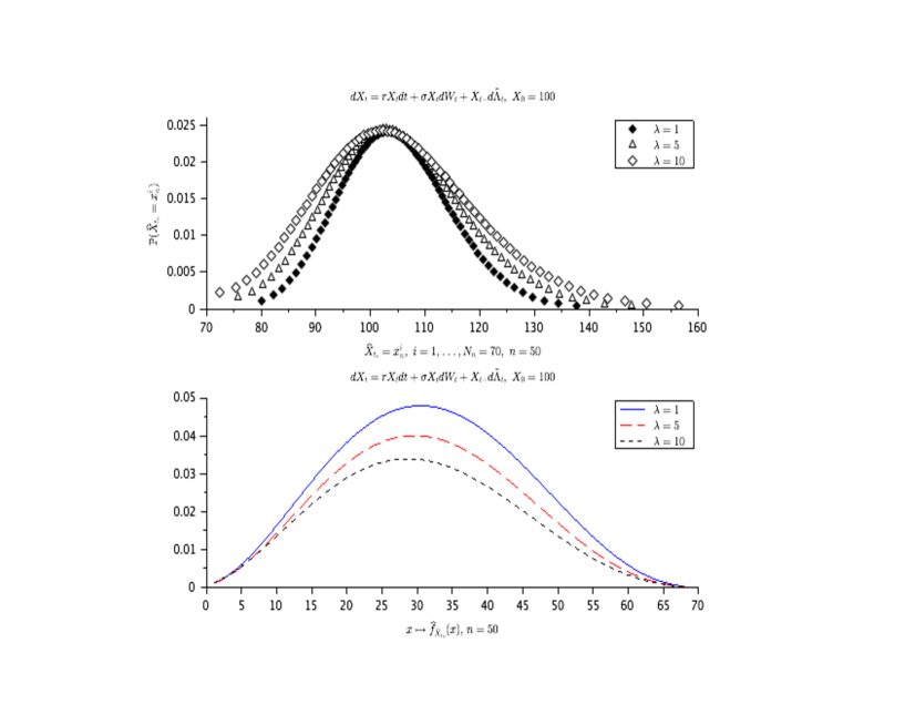
Figure 1: (impact of $\lambda$) The model is $dX_{t}=r\,X_{t}dt+\sigma X_{t}dW_{t}+X_{t-}d\tilde{\Lambda}_{t}$, $X_{0}=100$, $\tilde{\Lambda}_{t}=\sum_{i=1}^{\Lambda_{t}}U_{i}-\lambda t\mathbb{E}U_{1}$, where $U_{i}=e^{\xi_{i}}-1$ with $\xi_{i}={\cal N}(0;\vartheta^{2})$ and $\Lambda$ is a Poisson process with intensity $\lambda$. We choose $r=0.08$, $\sigma=0.108$, $\vartheta=0.04$, $T=0.5$. For the quantization, the number of discretization step $n=50$ and $N_{k}=70$, $\forall\,k=1,\ldots,n$. We compare de distributions of $\widehat{X}_{t_{n}}$ and the densities estimate functions $x\mapsto\hat{f}_{\bar{X}_{t_{n}}}(x)=2\,\mathbb{P}(\widehat{X}_{t_{n}}=x_{n}^{i})/(x_{n}^{i+1}-x_{n}^{i-1})\mathds{1}_{[x_{n}^{i-1},\ x_{n}^{i}]}(x)$, $\,x\in[x_{n}^{2},x_{n}^{N_{n}-1}]$, $n=50$, for $\lambda\in\{1,5,10\}$.

$\diamond$ Impact of $\lambda$ and $\vartheta$ on the marginal distributions of the stochastic process (42). Before dealing with the numerical experiments on the pricing, we want to see how the recursive quantization of the Euler scheme $(\bar{X}_{t_{k}})_{k=0,\ldots,n}$ looks like. To this end and to see the impact of the intensity $\lambda$ of the jumps on the marginal distributions of the stochastic process (42), we compare in Figure 1, the distributions of the recursive quantization $\widehat{X}_{t_{n}}$ and the associated (truncated) marginal densities approximate functions $\hat{f}_{\bar{X}_{t_{50}}}$, for the values of $\lambda\in\{1,5,10\}$. The truncated densities approximate function $\hat{f}_{\bar{X}_{t_{k}}}$ is defined on $[x_{k}^{2},x_{k}^{N_{k}-1}]$ as

$$\hat{f}_{X_{k}}(x)=\frac{2\,\mathbb{P}(\widehat{X}_{k}=x_{k}^{i})}{(x_{k}^{i+1}-x_{k}^{i-1})}\,\mathds{1}_{[x_{k}^{i-1},\ x_{k}^{i}]}(x),\qquad x\in[x_{k}^{2},x_{k}^{N_{k}-1}].$$

For the numerical tests we use the following set of parameters: $X_{0}=100$, $n=80$, $T=0.5$, $N_{k}=70$ for every $k=1,\ldots,n$ and $\widehat{X}_{0}=\mathds{1}_{\{x_{0}\}}$. We also set $r=0.08$, $\sigma=0.108$, $\vartheta=0.04$. The plots of Figure 1 show that the higher $\lambda$ is, the larger will be the tails (which are not represented in these plots) of the distributions of the marginals of the stochastic process (42).

​

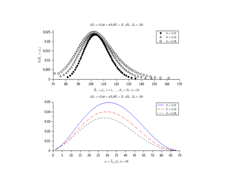
Figure 2: (Impact of $\vartheta$) The model is $dX_{t}=r\,X_{t}dt+\sigma X_{t}dW_{t}+X_{t-}d\tilde{\Lambda}_{t}$, $X_{0}=100$, $\tilde{\Lambda}_{t}=\sum_{i=1}^{\Lambda_{t}}U_{i}-\lambda t\mathbb{E}U_{1}$, where $U_{i}=e^{\xi_{i}}-1$ with $\xi_{i}={\cal N}(0;\vartheta^{2})$ and $\Lambda$ is a Poisson process with intensity $\lambda$. We choose $r=0.08$, $\sigma=0.108$, $\lambda=5$, $T=0.5$. For the quantization, the number of discretization step $n=50$ and $N_{k}=70$, $\forall\,k=1,\ldots,n$. We compare de distributions of $\widehat{X}_{t_{n}}$ and the densities estimate functions $x\mapsto\hat{f}_{\bar{X}_{t_{n}}}(x)=2\,\mathbb{P}(\widehat{X}_{t_{n}}=x_{n}^{i})/(x_{n}^{i+1}-x_{n}^{i-1})\mathds{1}_{[x_{n}^{i-1},\ x_{n}^{i}]}(x)$, $\,x\in[x_{n}^{2},x_{n}^{N_{n}-1}]$, $n=50$, for $\vartheta\in\{0.01,0.04,0.06\}$.

In Figure 2, we compare the same functions as in Figure 1 but this time by putting $\lambda=5$ and by making varying $\vartheta\in\{0.01,0.04,0.06\}$ to see the influence of the parameter $\vartheta$ on the marginal distributions of the stochastic process (42). As expected, we see once again that the higher $\vartheta$ is, the larger will be the tails of the distributions of the marginals of the stochastic process (42).

Remark that, compared with the model without jump, there are additional integral terms with respect to the distribution $\nu$ of the jump size when computing the gradient and the Hessian matrix of the distortion function. These integrals are approximated using the optimal quantization method of size $N=50$. This may increase a little bit the computation time w.r.t. to models without jump. In our example, we get all the marginal distributions with their associated weights in around 1min and 30s, using scilab software in a CPU 3.1 GHz and 16 Gb memory computer. Our aim here is just to test the performance of our method, not to optimize the execution time. However, it is clear that making the code in C program (even, optimizing the scilab code) will reduce drastically the computation time since their is many for loops in the actual code that increase the computation time.

$\diamond$ Pricing of a European put option with jump process using the recursive quantization. Let us come back to the pricing problem where our aim is to test the performance of the recursive quantization method. To this end, we compare the put price $\widehat{P}_{0}$ obtained from the recursive quantization method using the formula (44) with the true call price which formula is given from Equation (43). The comparison is done with the following set of parameters: $r=0.08$, $\sigma=0.07$, $T=0.5$, the number of discretization step $n=50$ and the size of the quantizations $N_{k}=100$, $\forall\,k=1,\ldots,n$, with $N_{0}=1$. We make varying $\lambda$ in the set values $\{1,3,5\}$, $\vartheta$ in the set $\{0.01,0.04\}$ and the strike $K$ in the set values $\{90,92,94,96,98,100\}$ and display the results in Table 1.

For matters of comparaison with the Black-Scholes model where the underlying asset price evolves following the dynamics $dX_{t}=rX_{t}dt+\sigma_{{}_{\rm BS}}dW_{t}$, a computation of ${\rm Var}(\ln(X_{t}))$ in both models allows us to write down $\sigma_{{}_{\rm BS}}$ (the equivalent volatility in the Black-Scholes model) with respect to $\sigma$: $\sigma_{{}_{\rm BS}}=\sqrt{\sigma^{2}+\lambda\vartheta^{2}}$.

The numerical results show a maximal absolute error of order $10^{-2}$ for a Black-Scholes equivalent volatility $\sigma_{{}_{\rm BS}}=0.1135782$ (obtained when $\lambda=5$ and $\vartheta=0.04$) and a minimal absolute error of order $10^{-3}$ for a Black-Scholes equivalent volatility $\sigma_{{}_{\rm BS}}=0.0707107$ (obtained with $\lambda=1$ and $\vartheta=0.01$). We also depict in Table 1 the true price $P_{{}_{\rm BS}}$ (and the approximate price $\widehat{P}_{{}_{\rm BS}}$ from the recursive quantization, see the numerical examples in [9] for more detail) of the put in the Black-Scholes model in order to compare it with the true price $P_{0}$ in the jump model (42). We see, as expected, that these two prices tend to coincide when $\lambda$ and $\vartheta$ are small.

Strike	$\lambda$	$P_{0}/\widehat{P}_{0}$ ($\vartheta=1\%$)	$P_{{}_{\rm BS}}/\widehat{P}_{{}_{\rm BS}}(\vartheta=1\%)$	$P_{0}/\widehat{P}_{0}$ ($\vartheta=4\%$)	$P_{{}_{\rm BS}}/\widehat{P}_{{}_{\rm BS}}(\vartheta=4\%)$
	1	0.002 / 0.002	0.002 / 0.002	0.015 / 0.013	0.009 / 0.008
90	3	0.003 / 0.002	0.003 / 0.002	0.057 / 0.055	0.043 / 0.041
	5	0.004 / 0.003	0.004 / 0.003	0.120 / 0.118	0.104 / 0.101
	1	0.010 / 0.009	0.010 / 0.009	0.037 / 0.036	0.029 / 0.027
92	3	0.012 / 0.011	0.012 / 0.115	0.115 / 0.114	0.100 / 0.098
	5	0.014 / 0.013	0.014 / 0.013	0.214 / 0.213	0.203 / 0.200
	1	0.035 / 0.035	0.036 / 0.035	0.087 / 0.087	0.080 / 0.078
94	3	0.041 / 0.040	0.040 / 0.040	0.218 / 0.218	0.211 / 0.207
	5	0.045 / 0.045	0.047 / 0.045	0.368 / 0.370	0.371 / 0.367
	1	0.103 / 0.105	0.107 / 0.105	0.193 / 0.196	0.193 / 0.190
96	3	0.117 / 0.113	0.116 / 0.115	0.396 / 0.405	0.406 / 0.402
	5	0.124 / 0.129	0.126 / 0.126	0.607 / 0.617	0.635 / 0.629
	1	0.259 / 0.270	0.270 / 0.267	0.356 / 0.407	0.414 / 0.410
98	3	0.289 / 0.280	0.290 / 0.286	0.684 / 0.704	0.724 / 0.719
	5	0.296 / 0.300	0.310 / 0.304	0.961 / 0.982	1.022 / 1.016
	1	0.566 / 0.585	0.589 / 0.585	0.751 / 0.775	0.796 / 0.791
100	3	0.593 / 0.610	0.617 / 0.613	1.121 / 1.159	1.200 / 1.194
	5	0.620 / 0.640	0.650 / 0.641	1.459 / 1.499	1.561 / 1.554

Table 1: The model is $dX_{t}=r\,X_{t}dt+\sigma X_{t}dW_{t}+X_{t-}d\tilde{\Lambda}_{t}$, $X_{0}=100$, $\tilde{\Lambda}_{t}=\sum_{i=1}^{\Lambda_{t}}U_{i}-\lambda t\mathbb{E}U_{1}$, where $U_{i}=e^{\xi_{i}}-1$ with $\xi_{i}={\cal N}(0;\vartheta^{2})$ and $\Lambda$ is a Poisson process with intensity $\lambda$. We choose $r=0.08$, $\sigma=0.07$, $T=0.5$. For the quantization, the number of discretization step $n=50$ and $N_{k}=100$, $\forall\,k=1,\ldots,n$. $P_{0}$ (resp. $P_{{}_{\rm BS}}$) is the true put price in the Merton model with jump (resp. without jump) and $\widehat{P}_{0}$ and $\widehat{P}_{{}_{\rm BS}}$ are their respective recursive quantization approximation.

Appendix A Proof of Lemma 2.1

Proof (of the key Lemma 2.1).

$(a)$ It follows from the elementary inequality

$$\forall u\!\in\mathbb{R}^{d},\quad|a+u|^{p}\leq|a|^{p}+p|a|^{p-2}(a|u)+\frac{p(p-1)}{2}\big{(}|a|^{p-2}|u|^{2}+|u|^{p}\big{)}$$

that

$$|a+\sqrt{h}A\zeta|^{p}\leq|a|^{p}+ph^{\frac{1}{2}}|a|^{p-2}(a|A\zeta)+\frac{p(p-1)}{2}\big{(}|a|^{p-2}h|A\zeta|^{2}+h^{\frac{p}{2}}|A\zeta|^{p}\big{)}.$$

Applying Young’s inequality with conjugate exponents $p^{\prime}=\frac{p}{p-2}$ and $q^{\prime}=\frac{p}{2}$, we get

$$|a|^{p-2}h|A\zeta|^{2}\leq h\Big{(}\frac{|a|^{p}}{p^{\prime}}+\frac{|A\zeta|^{p}}{q^{\prime}}\Big{)},$$

which leads to

$$|a+\sqrt{h}A\zeta|^{p} \leq |a|^{p}+ph^{\frac{1}{2}}|a|^{p-2}(a|A\zeta)+\frac{p(p-1)}{2}\Big{(}\frac{h}{p^{\prime}}|a|^{p}+\Big{(}\frac{h}{q^{\prime}}+h^{\frac{p}{2}}\Big{)}|A\zeta|^{p}\Big{)}$$

$$\leq |a|^{p}\Big{(}1+\frac{p(p-1)}{2p^{\prime}}h\Big{)}+ph^{\frac{1}{2}}|a|^{p-2}(a|A\zeta)+h\Big{(}\frac{p(p-1)}{2q^{\prime}}+h^{\frac{p}{2}-1}\Big{)}|A\zeta|^{p}.$$

Taking the expectation yields (owing to the fact that $\mathbb{E}\,\zeta=0$)

$$\mathbb{E}|a+\sqrt{h}A\zeta|^{p}\leq\Big{(}1+\frac{(p-1)(p-2)}{2}h\Big{)}|a|^{p}+h\Big{(}1+p+h^{\frac{p}{2}-1}\Big{)}\mathbb{E}|A\zeta|^{p}.$$

As a consequence, we get

$$\mathbb{E}|a+\sqrt{h}A\zeta|^{p}\leq\Big{(}1+\frac{(p-1)(p-2)}{2}h\Big{)}|a|^{p}+h\Big{(}1+p+h^{\frac{p}{2}-1}\Big{)}\|A\|^{p}\mathbb{E}|\zeta|^{p}.$$

$(b)$ It follows from the specified upper-bound of $a$ that (keep in mind that $p\!\in(2,3]$)

$$|a|^{p} \leq (1+2Lh)^{p}\Big{(}\frac{1+Lh}{1+2Lh}|x|+\frac{Lh}{1+2Lh}\Big{)}^{p}$$

$$\leq (1+2Lh)^{p}\Big{(}\frac{1+Lh}{1+2Lh}|x|^{p}+\frac{Lh}{1+2Lh}\Big{)}$$

$$\leq (1+2Lh)^{p}|x|^{p}+(1+2Lh)^{p-1}Lh.$$

Then, combining this with the specified upper-bound of $A$, we derive

$$\mathbb{E}|a+\sqrt{h}A\zeta|^{p} \leq \Big{(}1+\frac{(p-1)(p-2)}{2}h\Big{)}(1+2Lh)^{p}|x|^{p}$$

$$+\Big{(}1+\frac{(p-1)(p-2)}{2}h\Big{)}(1+2Lh)^{p-1}Lh$$

$$+h2^{p-1}\Lambda^{p}\Big{(}1+p+h^{\frac{p}{2}-1}\Big{)}(1+|x|^{p})\,\mathbb{E}|\zeta|^{p}.$$

Using the inequality $1+u\leq e^{u}$, for every $u\!\in\mathbb{R}$, we finally get

$$\mathbb{E}|a+\sqrt{h}A\zeta|^{p}\leq\Big{(}e^{\kappa_{p}h}+K_{p}h\Big{)}|x|^{p}+\big{(}e^{\kappa_{p}h}L+K_{p}\big{)}h,$$

where $\kappa_{p}:=\Big{(}\frac{(p-1)(p-2)}{2}+2pL\Big{)}$ and $K_{p}:=2^{p-1}\Lambda^{p}\Big{(}1+p+h^{\frac{p}{2}-1}\Big{)}\mathbb{E}|\zeta|^{p}$. ∎

Appendix B Gradient and Hessian of the recursive jump diffusion distortion when $\nu$ is Gaussian

Using some standard computations similar to [8] the components of the gradient vector of the distortion function read (in the short time framework) for every $j=1,\ldots,N_{k+1}$

$$\frac{\partial\tilde{D}_{k+1}(\Gamma_{k+1})}{\partial x_{k+1}^{j}} = 2\sum_{i=1}^{N_{k}}\sum_{m=0}^{1}p_{k}^{i}\,p_{m}\Big{[}\big{(}x_{k+1}^{j}-\mu_{k}(m,x_{k}^{i})\big{)}\Big{(}\Phi_{0}(x_{k+1}^{j+}(m,x_{k}^{i}))-\Phi_{0}(x_{k+1}^{j-}(m,x_{k}^{i}))\Big{)}$$

$$\qquad+\,v_{k}(m,x_{k}^{i})\big{(}\Phi_{0}^{\prime}(x_{k+1}^{j+}(m,x_{k}^{i}))-\Phi_{0}^{\prime}(x_{k+1}^{j-}(m,x_{k}^{i}))\big{)}\Big{]}.$$

The diagonal terms of the Hessian matrix $\nabla^{2}\widetilde{D}_{k+1}(\Gamma_{k+1})$ are given by:

$$\frac{\partial^{2}\tilde{D}_{k+1}(\Gamma_{k+1})}{\partial^{2}x_{k+1}^{j}}=2\sum_{i=1}^{N_{k}}\sum_{m=0}^{1} p_{k}^{i}\,p_{m}\Big{[} \Phi_{0}(x_{k+1}^{j+}(m,x_{k}^{i}))-\Phi_{0}(x_{k+1}^{j-}(m,x_{k}^{i}))$$

$$-\frac{1}{4v_{k}(m,x_{k}^{i})}\Phi_{0}^{\prime}(x_{k+1}^{j+}(m,x_{k}^{i}))(x_{k+1}^{j+1}-x_{k+1}^{j})$$

$$-\frac{1}{4v_{k}(m,x_{k}^{i})}\Phi_{0}^{\prime}(x_{k+1}^{j-}(m,x_{k}^{i}))(x_{k+1}^{j}-x_{k+1}^{j-1})\Big{]}$$

and its sub-diagonal terms are

$$\frac{\partial^{2}\tilde{D}_{k+1}(\Gamma_{k+1})}{\partial x_{k+1}^{j}\partial x_{k+1}^{j-1}}=-\frac{1}{2}\sum_{i=1}^{N_{k}}\sum_{m=0}^{1}p_{k}^{i}\,p_{m}\frac{1}{v_{k}(m,x_{k}^{i})}(x_{k+1}^{j}-x_{k+1}^{j-1})\Phi_{0}^{\prime}(x_{k+1}^{j-}(m,x_{k}^{i})).$$

The upper-diagonals terms are

$$\frac{\partial^{2}\tilde{D}_{k+1}(\Gamma_{k+1})}{\partial x_{k+1}^{j}\partial x_{k+1}^{j+1}}=-\frac{1}{2}\sum_{i=1}^{N_{k}}\sum_{m=0}^{1}p_{k}^{i}\,p_{m}\frac{1}{v_{k}(m,x_{k}^{i})}(x_{k+1}^{j+1}-x_{k+1}^{j})\Phi_{0}^{\prime}(x_{k+1}^{j+}(m,x_{k}^{i})).$$

Appendix C Gradient and Hessian of the recursive jump diffusion distortion for a general $\nu$

In this case, the components of the gradient vector of the distortion function read for every $j=1,\ldots,N_{k+1}$

$$\frac{\partial\tilde{D}_{k+1}(\Gamma_{k+1})}{\partial x_{k+1}^{j}} = 2\sum_{i=1}^{N_{k}}\sum_{m=0}^{1}p_{k}^{i}\,p_{m}\int_{\mathbb{R}}\nu(du)\Big{[}\big{(}x_{k+1}^{j}-\mu_{k}(m,x_{k}^{i},u)\big{)}\Big{(}\Phi_{0}(x_{k+1}^{j+}(m,x_{k}^{i},u))$$

$$\ -\,\Phi_{0}\big{(}x_{k+1}^{j-}(m,x_{k}^{i},u)\big{)}\Big{)}+v_{k}(x_{k}^{i})\big{(}\Phi_{0}^{\prime}(x_{k+1}^{j+}(m,x_{k}^{i},u))-\Phi_{0}^{\prime}(x_{k+1}^{j-}(m,x_{k}^{i},u))\big{)}\Big{]}.$$

The diagonal terms of the Hessian matrix $\nabla^{2}\tilde{D}_{k+1}(\Gamma_{k+1})$ are given by:

$$\frac{\partial^{2}\tilde{D}_{k+1}(\Gamma_{k+1})}{\partial^{2}x_{k+1}^{j}} = 2\sum_{i=1}^{N_{k}}\sum_{m=0}^{1}p_{k}^{i}\,p_{m}\int_{\mathbb{R}}\nu(du)\Big{[}\Phi_{0}(x_{k+1}^{j+}(m,x_{k}^{i},u))-\Phi_{0}(x_{k+1}^{j-}(m,x_{k}^{i},u))$$

$$\hskip 113.81102pt\,-\,\frac{1}{4v_{k}(x_{k}^{i})}\Phi_{0}^{\prime}(x_{k+1}^{j+}(m,x_{k}^{i},u))(x_{k+1}^{j+1}-x_{k+1}^{j})$$

$$\hskip 113.81102pt\,-\,\frac{1}{4v_{k}(x_{k}^{i})}\Phi_{0}^{\prime}(x_{k+1}^{j-}(m,x_{k}^{i},u))(x_{k+1}^{j}-x_{k+1}^{j-1})\Big{]}$$

and its sub-diagonal terms are

$$\frac{\partial^{2}\tilde{D}_{k+1}(\Gamma_{k+1})}{\partial x_{k+1}^{j}\partial x_{k+1}^{j-1}}=-\frac{1}{2}\sum_{i=1}^{N_{k}}\sum_{m=0}^{1}p_{k}^{i}\,p_{m}\frac{1}{v_{k}(x_{k}^{i})}(x_{k+1}^{j}-x_{k+1}^{j-1})\int_{\mathbb{R}}\Phi_{0}^{\prime}(x_{k+1}^{j-}(m,x_{k}^{i},u))\nu(du).$$

The upper-diagonals terms are

$$\frac{\partial^{2}\tilde{D}_{k+1}(\Gamma_{k+1})}{\partial x_{k+1}^{j}\partial x_{k+1}^{j+1}}=-\frac{1}{2}\sum_{i=1}^{N_{k}}\sum_{m=0}^{1}p_{k}^{i}\,p_{m}\frac{1}{v_{k}(x_{k}^{i})}(x_{k+1}^{j+1}-x_{k+1}^{j})\int_{\mathbb{R}}\Phi_{0}^{\prime}(x_{k+1}^{j+}(m,x_{k}^{i},u))\nu(du).$$

The involved functions are defined as follows: $\mu_{k}(m,x,u)=x+h\,b(t_{k},x)+(mu-\lambda h\,\mathbb{E}(U_{1}))\gamma(x)$ and $v_{k}(x)=\sqrt{h}\,\sigma(t_{k},x)$. Like previously, we set

$$x_{k+1}^{j-}(m,x,u):=\frac{x_{k+1}^{j-1/2}-\mu_{k}(m,x,u)}{v_{k}(x)}\ \textrm{ and }\ x_{k+1}^{j+}(m,x,u):=\frac{x_{k+1}^{j+1/2}-\mu_{k}(m,x,u)}{v_{k}(x)},\;k=0,\ldots,n-1.$$

References

• [1] G. Callegaro, L. Fiorin, and M. Grasselli. Quantized calibration in local volatility. Risk Magazine, 28(4):62 – 67, 2015.
• [2] G. Callegaro, L. Fiorin, and M. Grasselli. Pricing via recursive quantization in stochastic volatility models. Quantitative Finance, Online version:1–18, 2016.
• [3] G. Callegaro, L. Fiorin, and M. Grasselli. Quantization meets Fourier: A new technology for pricing options. Quantitative Finance, Online version, 2017.
• [4] L. Fiorin, G. Pagès, and A. Sagna. Product markovian quantization of a diffusion process with applications to finance. Methodology and Computing in Applied Probability. To appear., 2018.
• [5] S. Graf and H. Luschgy. Foundations of Quantization for Probability Distributions. Lect. Notes in Math. 1730. Springer, Berlin., 2000.
• [6] P. E. Kloeden and E. Platen. Numerical Solution of Stochastic Differential Equations. Springer, Verlag., 1992.
• [7] H. Luschgy and G. Pagès. Functional quantization rate and mean regularity of processes with an application to lévy processes. Annals of Applied Probability, 18(2):427–469, 2008.
• [8] G. Pagès and A. Sagna. Asymptotics of the maximal radius of an ${L}^{r}$-optimal sequence of quantizers. Bernoulli, 18(1):360–389, 2012.
• [9] G. Pagès and A. Sagna. Recursive marginal quantization of the euler scheme of a diffusion process. Applied Mathematical Finance., 22(15):463–498, 2015.
• [10] Gilles Pagès. Numerical probability: an introduction with application to Finance. Universitext. Springer-Verlag, 2017. Springer.
• [11] R. Ralf. Recursive Marginal Quantization: Extensions and Applications in Finance. PhD thesis, Univ. Cape Town, 2018.
• [12] A. M. Thomas, Ralph Rudd, Jörg K., and Eckhard P. Recursive marginal quantization of high-order scheme. Preprint, 0:0, 2017.