Online ICA: Understanding Global Dynamics of Nonconvex Optimization via Diffusion Processes

Abstract

Solving statistical learning problems often involves nonconvex optimization. Despite the empirical success of nonconvex statistical optimization methods, their global dynamics, especially convergence to the desirable local minima, remain less well understood in theory. In this paper, we propose a new analytic paradigm based on diffusion processes to characterize the global dynamics of nonconvex statistical optimization. As a concrete example, we study stochastic gradient descent (SGD) for the tensor decomposition formulation of independent component analysis. In particular, we cast different phases of SGD into diffusion processes, i.e., solutions to stochastic differential equations. Initialized from an unstable equilibrium, the global dynamics of SGD transit over three consecutive phases: (i) an unstable Ornstein-Uhlenbeck process slowly departing from the initialization, (ii) the solution to an ordinary differential equation, which quickly evolves towards the desirable local minimum, and (iii) a stable Ornstein-Uhlenbeck process oscillating around the desirable local minimum. Our proof techniques are based upon Stroock and Varadhan’s weak convergence of Markov chains to diffusion processes, which are of independent interest.

1 Introduction

For solving a broad range of large-scale statistical learning problems, e.g., deep learning, nonconvex optimization methods often exhibit favorable computational and statistical efficiency empirically. However, there is still a lack of theoretical understanding of the global dynamics of these nonconvex optimization methods. In specific, it remains largely unexplored why simple optimization algorithms, e.g., stochastic gradient descent (SGD), often exhibit fast convergence towards local minima with desirable statistical accuracy. In this paper, we aim to develop a new analytic framework to theoretically understand this phenomenon.

The dynamics of nonconvex statistical optimization are of central interest to a recent line of work. Specifically, by exploring the local convexity within the basins of attraction, [26, 35, 1, 5, 52, 53, 36, 22, 25, 11, 7, 56, 39, 20, 47, 31, 46, 6, 57, 12, 50, 13, 8, 54, 58, 10, 24, 51, 55, 48, 21, 49] establish local fast rates of convergence towards the desirable local minima for a variety statistical problems. Most of these characterizations of local dynamics are based on two decoupled ingredients from statistics and optimization: (i) the local (approximately) convex geometry of the objective functions, which is induced by the underlying statistical models, and (ii) adaptation of classical optimization analysis [34, 19] by incorporating the perturbations induced by nonconvex geometry as well as random noise. To achieve global convergence guarantees, they rely on various problem-specific approaches to obtain initializations that provably fall into the basins of attraction. Meanwhile, for some learning problems, such as phase retrieval and tensor decomposition for latent variable models, it is empirically observed that good initializations within the basins of attraction are not essential to the desirable convergence. However, it remains highly challenging to characterize the global dynamics, especially within the highly nonconvex regions outside the local basins of attraction.

In this paper, we address this problem with a new analytic framework based on diffusion processes. In particular, we focus on the concrete example of SGD applied on the tensor decomposition formulation of independent component analysis (ICA). Instead of adapting classical optimization analysis accordingly to local nonconvex geometry, we cast SGD in different phases as diffusion processes, i.e., solutions to stochastic differential equations (SDE), by analyzing the weak convergence from discrete Markov chains to their continuous-time limits [40, 17]. The SDE automatically incorporates the geometry and randomness induced by the statistical model, which allows us to establish the exact dynamics of SGD. In contrast, classical optimization analysis only yields upper bounds on the optimization error, which are unlikely to be tight in the presence of highly nonconvex geometry, especially around the stationary points that have negative curvatures along certain directions. In particular, we identify three consecutive phases of the global dynamics of SGD, which is illustrated in Figure 1.

1. We consider the most challenging initialization at a stationary point with negative curvatures, which can be cast as an unstable equilibrium of the SDE. Within the first phase, the dynamics of SGD are characterized by an unstable Ornstein-Uhlenbeck process [37, 2], which departs from the initialization at a relatively slow rate and enters the second phase.

2. Within the second phase, the dynamics of SGD are characterized by the exact solution to an ordinary differential equation. This solution evolves towards the desirable local minimum at a relatively fast rate until it approaches a small basin around the local minimum.

3. Within the third phase, the dynamics of SGD are captured by a stable Ornstein-Uhlenbeck process [37, 2], which oscillates within a small basin around the local minimum.

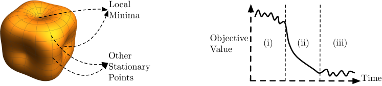
Figure 1: Left: an illustration of the objective function for the tensor decomposition formulation of ICA. Note that here we use the spherical coordinate system and add a global offset of $2$ to the objective function for better illustration. Right: An illustration of the three phases of diffusion processes.

More related work. Our results are connected with a very recent line of work [18, 42, 43, 44, 45, 27, 29, 3, 38] on the global dynamics of nonconvex statistical optimization. In detail, they characterize the global geometry of nonconvex objective functions, especially around their saddle points or local maxima. Based on the geometry, they prove that specific optimization algorithms, e.g., SGD with artificial noise injection, gradient descent with random initialization, and second-order methods, avoid the saddle points or local maxima, and globally converge to the desirable local minima. Among these results, our results are most related to [18], which considers SGD with noise injection on ICA. Compared with this line of work, our analysis takes a completely different approach based on diffusion processes, which is also related to another line of work [14, 15, 41, 30, 33, 32].

Without characterizing the global geometry, we establish the global exact dynamics of SGD, which illustrate that, even starting from the most challenging stationary point, it may be unnecessary to use additional techniques such as noise injection, random initialization, and second-order information to ensure the desirable convergence. In other words, the unstable Ornstein-Uhlenbeck process within the first phase itself is powerful enough to escape from stationary points with negative curvatures. This phenomenon is not captured by the previous upper bound-based analysis, since previous upper bounds are relatively coarse-grained compared with the exact dynamics, which naturally give a sharp characterization simultaneously from upper and lower bounds. Furthermore, in Section 5 we will show that our sharp diffusion process-based characterization provides understanding on different phases of dynamics of our online/SGD algorithm for ICA.

A recent work [29] analyzes an online principal component analysis algorithm based on the intuition gained from diffusion approximation. In this paper, we consider a different statistical problem with a rigorous characterization of the diffusion approximations in three separate phases.

Our contribution. In summary, we propose a new analytic paradigm based on diffusion processes for characterizing the global dynamics of nonconvex statistical optimization. For SGD on ICA, we identify the aforementioned three phases for the first time. Our analysis is based on Stroock and Varadhan’s weak convergence of Markov chains to diffusion processes, which are of independent interest.

2 Background

In this section we formally introduce a special model of independent component analysis (ICA) and the associated SGD algorithm. Let $\{\bm{X}^{(i)}\}_{i=1}^{n}$ be the data sample identically distributed as $\bm{X}\in\mathbb{R}^{d}$. We make assumptions for the distribution of $\bm{X}$ as follows. Let $\|\cdot\|$ be the $\ell_{2}$-norm of a vector.

Assumption 1.

There is an orthonormal matrix $\mathbf{A}\in\mathbb{R}^{d\times d}$ such that $\bm{X}=\mathbf{A}\bm{Y}$, where $\bm{Y}\in\mathbb{R}^{d}$ is a random vector that has independent entries satisfying the following conditions:

1. The distribution of each $Y_{i}$ is symmetric about 0;

2. There is a constant $B$ such that $\|\bm{Y}\|^{2}\leq B$;

3. The $Y_{1},\ldots,Y_{d}$ are independent with identical $m$ moments for $m\leq 8$, denoted by $\psi_{m}\equiv\mathbb{E}Y_{1}^{m}$;

4. The $\psi_{1}=\mathbb{E}Y_{i}=0$, $\psi_{2}=\mathbb{E}Y_{i}^{2}=1$, $\psi\equiv\psi_{4}\neq 3$.

Assumption 1(iii) above is a generalization of i.i.d. tensor components. Let $\mathbf{A}=\left(\mathbf{a}_{1},\ldots,\mathbf{a}_{d}\right)$ whose columns form an orthonormal basis. Our goal is to estimate the orthonormal basis $\mathbf{a}_{i}$ from online data $\bm{X}_{1},\ldots,\bm{X}_{n}$. We first establish a preliminary lemma.

Lemma 1.

Let $\mathbf{T}\!=\!\mathbb{E}(\bm{X}^{\otimes 4})$ be the 4th-order tensor whose $(i,j,k,l)$-entry is $\mathbb{E}\left(X_{i}X_{j}X_{k}X_{l}\right)$. Under Assumption 1, we have

$$\mathbf{T}(\mathbf{u},\mathbf{u},\mathbf{u},\mathbf{u})\equiv\mathbb{E}\left(\mathbf{u}^{\top}\bm{X}\right)^{4}=3+(\psi-3)\sum_{i=1}^{d}(\mathbf{a}_{i}^{\top}\mathbf{u})^{4}.$$ (2.1)

Lemma 1 implies that finding $\mathbf{a}_{i}$’s can be cast into the solution to the following population optimization problem

$${\rm argmin}-\mathop{\mathrm{sign}}(\psi-3)\cdot\mathbb{E}\left(\mathbf{u}^{\top}\bm{X}\right)^{4}={\rm argmin}\sum_{i=1}^{d}-(\mathbf{a}_{i}^{\top}\mathbf{u})^{4}\leavevmode\nobreak\ \leavevmode\nobreak\ \leavevmode\nobreak\ \leavevmode\nobreak\ \leavevmode\nobreak\ \mbox{subject to }\|\mathbf{u}\|=1.$$ (2.2)

It is straightforward to conclude that all stable equilibria of (2.2) are $\pm\mathbf{a}_{i}$ whose number linearly grows with $d$. Meanwhile, by analyzing the Hessian matrices the set of unstable equilibria of (2.2) includes (but not limited to) all $\mathbf{v}^{*}=d^{-1/2}(\pm 1,\cdots,\pm 1)$, whose number grows exponentially as $d$ increases [18, 44].

Now we introduce the SGD algorithm for solving (2.2) with finite samples. Let ${\mathcal{S}}^{d-1}=\{\mathbf{u}:\|\mathbf{u}\|=1\}$ be the unit sphere in $\mathbb{R}^{d}$, and denote $\Pi\mathbf{u}=\mathbf{u}/\|\mathbf{u}\|$ for $\mathbf{u}\neq 0$ the projection operator onto ${\mathcal{S}}^{d-1}$. With appropriate initialization, the SGD for tensor method iteratively updates the estimator via the following Eq. (2.3):

$$\mathbf{u}^{(n)}=\Pi\left\{\mathbf{u}^{(n-1)}+\mathop{\mathrm{sign}}(\psi-3)\cdot\beta\left(\mathbf{u}^{(n-1)}\,{}^{\top}\bm{X}^{(n)}\right)^{3}\bm{X}^{(n)}\right\}.$$ (2.3)

The SGD algorithms that performs stochastic approximation using single online data sample in each update has the advantage of less temporal and spatial complexity, especially when $d$ is high [29, 18]. An essential issue of this nonconvex optimization problem is how the algorithm escape from unstable equilibria. [18] provides a method of adding artificial noises to the samples, where the noise variables are uniformly sampled from ${\mathcal{S}}^{d-1}$. In our work, we demonstrate that under some reasonable distributional assumptions, the online data provide sufficient noise for the algorithm to escape from the unstable equilibria.

By symmetry, our algorithm in Eq. (2.3) converges to a uniformly random tensor component from $d$ components. In order to solve the problem completely, one can repeatedly run the algorithm using different set of online samples until all tensor components are found. In the case where $d$ is high, the well-known coupon collector problem [16] implies that it takes $\approx d\log d$ runs of SGD algorithm to obtain all $d$ tensor components.

Remark.

From Eq. (2.2) we see the tensor structure in Eq. (2.1) is unidentifiable in the case of $\psi=3$, see more discussion in [4, 18]. Therefore in Assumption 1 we rule out the value $\psi=3$ and call the value $\left|\psi-3\right|$ the tensor gap. The reader will see later that, analogous to eigengap in SGD algorithm for principal component analysis (PCA) [29], tensor gap plays a vital role in the time complexity in the algorithm analysis.

3 Markov Processes and Differential Equation Approximation

To work on the approximation we first conclude the following proposition.

Proposition 1.

The iteration $\mathbf{u}^{(n)},n=0,1,\ldots$ generated by Eq. (2.3) forms a discrete-time, time-homogeneous Markov process that takes values on ${\mathcal{S}}^{d-1}$. Furthermore, $\mathbf{u}^{(n)}$ holds strong Markov property.

For convenience of analysis we use the transformed iteration $\mathbf{v}^{(n)}\equiv\mathbf{A}^{\top}\mathbf{u}^{(n)}$ in the rest of this paper. The update equation in Eq. (2.3) is equivalently written as

$$\begin{split}\mathbf{v}^{(n)}=\mathbf{A}^{\top}\mathbf{u}^{(n)}&=\Pi\left\{\mathbf{A}^{\top}\mathbf{u}^{(n-1)}\pm\beta\left(\mathbf{u}^{(n-1)}\,{}^{\top}\mathbf{A}\mathbf{A}^{\top}\bm{X}^{(n)}\right)^{3}\mathbf{A}^{\top}\bm{X}^{(n)}\right\}\\ &=\Pi\left\{\mathbf{v}^{(n-1)}\pm\beta\left(\mathbf{v}^{(n-1)}\,{}^{\top}\bm{Y}^{(n)}\right)^{3}\bm{Y}^{(n)}\right\}.\end{split}$$ (3.1)

Here $\pm\beta$ has the same sign with $\psi-3$. It is obvious from Proposition 1 that the (strong) Markov property applies to $\mathbf{v}^{(n)}$, and one can analyze the iterates $\mathbf{v}^{(n)}$ generated by Eq. (3.1) from a perspective of Markov processes.

Our next step is to conclude that as the stepsize $\beta\rightarrow 0^{+}$, the iterates generated by Eq. (2.3), under the time scaling that speeds up the algorithm by a factor $\beta^{-1}$, can be globally approximated by the solution to the following ODE system. To characterize such approximation we use theory of weak convergence to diffusions [40, 17] via computing the infinitesimal mean and variance for SGD for the tensor method. We remind the readers of the definition of weak convergence $Z^{\beta}\Rightarrow Z$ in stochastic processes: for any $0\leq t_{1}<t_{2}<\cdots<t_{n}$ the following convergence in distribution occurs as $\beta\rightarrow 0^{+}$

$$\left(Z^{\beta}(t_{1}),Z^{\beta}(t_{2}),\ldots,Z^{\beta}(t_{n})\right)\stackrel{{\scriptstyle\scriptstyle d}}{{\longrightarrow}}\left(Z(t_{1}),Z(t_{2}),\ldots,Z(t_{n})\right).$$

To highlight the dependence on $\beta$ we add it in the superscipts of iterates $\mathbf{v}^{\beta,(n)}=\mathbf{v}^{(n)}$. Recall that $\lfloor t\beta^{-1}\rfloor$ is the integer part of the real number $t\beta^{-1}$.

Theorem 1.

If for each $k=1,\ldots,d$, as $\beta\rightarrow 0^{+}$ $v_{k}^{\beta,(0)}$ converges weakly to some constant scalar $V_{k}^{o}$ then the Markov process $v_{k}^{\beta,(\lfloor t\beta^{-1}\rfloor)}$ converges weakly to the solution of the ODE system

$$\frac{{\mathrm{d}}V_{k}}{{\mathrm{d}}t}=\left|\psi-3\right|V_{k}\left(V_{k}^{2}-\sum_{i=1}^{d}V_{i}^{4}\right),\qquad k=1,\ldots,d,$$ (3.2)

with initial values $V_{k}(0)=V_{k}^{o}$.

To understand the complex ODE system in Eq. (3.2) we first investigate into the case of $d=2$. Consider a change of variable $V_{1}^{2}(t)$ we have by chain rule in calculus and $V_{2}^{2}=1-V_{1}^{2}$ the following derivation:

$$\frac{{\mathrm{d}}V_{1}^{2}}{{\mathrm{d}}t} =2V_{1}\cdot\frac{{\mathrm{d}}V_{1}}{{\mathrm{d}}t}=2V_{1}\cdot\left|\psi-3\right|V_{1}\left(V_{1}^{2}-V_{1}^{4}-V_{2}^{4}\right)$$

$$=2\left|\psi-3\right|V_{1}^{2}\left(V_{1}^{2}-V_{1}^{4}-(1-V_{1}^{2})^{2}\right)=-2\left|\psi-3\right|V_{1}^{2}\left(V_{1}^{2}-\frac{1}{2}\right)(V_{1}^{2}-1).$$ (3.3)

Eq. (3.3) is an autonomous, first-order ODE for $V_{1}^{2}$. Although this equation is complex, a closed-form solution is available:

$$V_{1}^{2}(t)=0.5\pm 0.5(1+C\exp\left(-|\psi-3|t\right))^{-0.5},$$

and $V_{2}^{2}(t)=1-V_{1}^{2}(t)$, where the choices of $\pm$ and $C$ depend on the initial value. The above solution allows us to conclude that if the initial vector $(V_{1}^{o})^{2}<(V_{2}^{o})^{2}$ (resp. $(V_{1}^{o})^{2}>(V_{2}^{o})^{2}$), then it approaches to 1 (resp. 0) as $t\rightarrow\infty$. This intuition can be generalized to the case of higher $d$ that the ODE system in Eq. (3.2) converges to the coordinate direction $\pm\mathbf{e}_{k}$ if $(V_{k}^{o})^{2}$ is strictly maximal among $(V_{1}^{o})^{2},\ldots,(V_{d}^{o})^{2}$ in the initial vector. To estimate the time of traverse we establish the following Proposition 2.

Proposition 2.

Fix $\delta\in(0,1/2)$ and the initial value $V_{k}(0)=V_{k}^{o}$ that satisfies $(V_{k_{0}}^{o})^{2}\geq 2(V_{k}^{o})^{2}$ for all $1\leq k\leq d,k\neq k_{0}$, then there is a constant (called traverse time) $T$ that depends only on $d,\delta$ such that $V_{k_{0}}^{2}(T)\geq 1-\delta.$ Furthermore $T$ has the following upper bound: let $y(t)$ solution to the following auxillary ODE

$$\frac{{\mathrm{d}}y}{{\mathrm{d}}t}=y^{2}\left(1-y\right),$$ (3.4)

with $y(0)=2/(d+1)$. Let $T_{0}$ be the time that $y(T_{0})=1-\delta$. Then

$$T\leq|\psi-3|^{-1}T_{0}\leq|\psi-3|^{-1}\left(d-3+4\log(2\delta)^{-1}\right).$$ (3.5)

Proposition 2 concludes that, by admitting a gap of $2$ between the largest $(V_{k_{0}}^{o})^{2}$ and second largest $(V_{k}^{o})^{2}$, $k\neq k_{0}$ the estimate on traverse time can be given, which is tight enough for our purposes in Section 5.

Remark.

In an earlier paper [29] which focuses on the SGD algorithm for PCA, when the stepsize is small, the algorithm iteration is approximated by the solution to ODE system after appropriate time rescaling. The approximate ODE system for SGD for PCA is

$$\frac{{\mathrm{d}}V_{k}}{{\mathrm{d}}t}=-2V_{k}\sum_{i=1}^{d}(\lambda_{k}-\lambda_{i})V_{i}^{2},\qquad k=1,\ldots,d.$$ (3.6)

The analysis there also involves computation of infinitesimal mean and variance for each coordinate as the stepsize $\beta\rightarrow 0^{+}$ and theory of convergence to diffusions [40, 17]. A closed-form solution to Eq. (3.6) is obtained in [29], called the generalized logistic curves. In contrast, to our best knowledge a closed-form solution to Eq. (3.2) is generally not available.

4 Local Approximation via Stochastic Differential Equation

The ODE approximation in Section 3 is very informative: it characterizes globally the trajectory of our algorithm for ICA or tensor method in Eq. (2.3) with $\mathcal{O}(1)$ approximation errors. However it fails to characterize the behavior near equilibria where the gradients in our ODE system are close to zero. For instance, if the SGD algorithm starts from $\mathbf{v}^{*}$, on a microscopic magnitude of $\mathcal{O}(\beta^{1/2})$ the noises generated by online samples help escaping from a neighborhood of $\mathbf{v}^{*}$.

Our main goal in this section is to demonstrate that under appropriate spatial and temporal scalings, the algorithm iteration converges locally to the solution to certain stochastic differential equations (SDE). We provide the SDE approximations in two scenarios, separately near an arbitrary tensor component (Subsection 4.1) which indicates that our SGD for tensor method converges to a local minimum at a desirable rate, and a special local maximum (Subsection 4.2) which implies that the stochastic nature of our SGD algorithm for tensor method helps escaping from unstable equilibria. Note that in the algorithm iterates, the escaping from stationary points occurs first, followed by the ODE and then by the phase of convergence to local minimum. We discuss this further in Section 5.

4.1 Neighborhood of Local Minimizers

To analyze the behavior of SGD for tensor method we first consider the case where the iterates enter a neighborhood of one local minimizer, i.e. the tensor component. Since the tensor decomposition in Eq. (2.2) is full-rank and symmetric, we consider without loss of generality the neighborhood near $\mathbf{e}_{1}$ the first tensor component. The following Theorem 2 indicates that under appropriate spatial and temporal scalings, the process admits an approximation by Ornstein-Uhlenbeck process. Such approximation is characterized rigorously using weak convergence theory of Markov processes [40, 17]. The readers are referred to [37] for fundamental topics on SDE.

Theorem 2.

If for each $k=2,\ldots,d$, $\beta^{-1/2}v_{k}^{\beta,(0)}$ converges weakly to $U_{k}^{o}\in(0,\infty)$ as $\beta\rightarrow 0^{+}$ then the stochastic process $\beta^{-1/2}v_{k}^{\beta,(\lfloor t\beta^{-1}\rfloor)}$ converges weakly to the solution of the stochastic differential equation

$${\mathrm{d}}U_{k}(t)=-\left|\psi-3\right|U_{k}(t){\mathrm{d}}t+\psi_{6}^{1/2}{\mathrm{d}}B_{k}(t),$$ (4.1)

with initial values $U_{k}(0)=U_{k}^{o}$. Here $B_{k}(t)$ is a standard one-dimensional Brownian motion.

We identify the solution to Eq. (4.1) as an Ornstein-Uhlenbeck process which can be expressed in terms of a Itô integral, with

$$U_{k}(t)=U_{k}^{o}\exp\left(-|\psi-3|t\right)+\psi_{6}^{1/2}\int_{0}^{t}\exp\left(-|\psi-3|(t-s)\right){\mathrm{d}}B_{k}(s).$$ (4.2)

Itô isometry along with mean-zero property of Itô integral gives

$$\mathbb{E}(U_{k}(t))^{2} =(U_{k}^{o})^{2}\exp\left(-2|\psi-3|t\right)+\psi_{6}\int_{0}^{t}\exp\left(-2|\psi-3|(t-s)\right){\mathrm{d}}s$$

$$=\frac{\psi_{6}}{2|\psi-3|}+\left((U_{k}^{o})^{2}-\frac{\psi_{6}}{2|\psi-3|}\right)\exp\left(-2|\psi-3|t\right),$$

which, by taking the limit $t\rightarrow\infty$, approaches $\psi_{6}/(2|\psi-3|)$. From the above analysis we conclude that the Ornstein-Uhlenbeck process has the mean-reverting property that its mean decays exponentially towards 0 with persistent fluctuations at equilibrium.

4.2 Escape from Unstable Equilibria

In this subsection we consider SGD for tensor method that starts from a sufficiently small neighborhood of a special unstable equilibrium. We show that after appropriate rescalings of both time and space, the SGD for tensor iteration can be approximated by the solution to a second SDE. Analyzing the approximate SDE suggests that our SGD algorithm iterations can get rid of the unstable equilibria (including local maxima and stationary points with negative curvatures) whereas the traditional gradient descent (GD) method gets stuck. In other words, under weak distributional assumptions the stochastic gradient plays a vital role that helps the escape. As a illustrative example, we consider the special stationary points $\mathbf{v}^{*}=d^{-1/2}(\pm 1,\ldots,\pm 1)$. Consider a submanifold ${\mathcal{S}}_{F}\subseteq{\mathcal{S}}^{d-1}$ where

$${\mathcal{S}}_{F}=\left\{\mathbf{v}\in{\mathcal{S}}^{d-1}:\mbox{there exists $1\leq k<k^{\prime}\leq d$ such that $v_{k}^{2}=v_{k^{\prime}}^{2}=\max_{1\leq i\leq d}v_{i}^{2}$}\right\}.$$

In words, ${\mathcal{S}}_{F}$ consists of all $\mathbf{v}\in{\mathcal{S}}^{d-1}$ where the maximum of $v_{k}^{2}$ is not unique. In the case of $d=3$, it is illustrated by Figure 1 that ${\mathcal{S}}_{F}$ is the frame of a 3-dimenisional box, and hence we call ${\mathcal{S}}_{F}$ the frame. Let

$$W^{\beta}_{kk^{\prime}}(t)=\beta^{-1/2}\log\big{(}v_{k}^{\beta,(\lfloor t\beta^{-1}\rfloor)}\big{)}^{2}-\beta^{-1/2}\log\big{(}v_{k^{\prime}}^{\beta,(\lfloor t\beta^{-1}\rfloor)}\big{)}^{2}.$$ (4.3)

The reason we study $W^{\beta}_{kk^{\prime}}(t)$ is that these $d(d-1)$ functions of $\mathbf{v}\in{\mathcal{S}}^{d-1}$ form a local coordinate map around $\mathbf{v}^{*}$ and further characterize the distance between $\mathbf{v}$ and ${\mathcal{S}}_{F}$ on a spatial scale of $\beta^{1/2}$. We define the positive constant $\Lambda_{d,\psi}$ as

$$\begin{split}\Lambda_{d,\psi}^{2}&=8d^{-2}\left(\psi_{8}+(16d-28)\psi_{6}+15d\psi_{4}^{2}\right.\\ &\quad\left.-5(72d^{2}-228d+175)\psi_{4}+15(2d-7)(d-2)(d-3)\right).\end{split}$$ (4.4)

We have our second SDE approximation result as follows.

Theorem 3.

Let $W^{\beta}_{kk^{\prime}}(t)$ be defined as in Eq. (4.3), and let $\Lambda_{d,\psi}$ be as in Eq. (4.4). If for each distinct $k,k^{\prime}=1,\ldots,d$, $W^{\beta}_{kk^{\prime}}(0)$ converges weakly to $W_{kk^{\prime}}^{o}\in(0,\infty)$ as $\beta\rightarrow 0^{+}$ then the stochastic process $W^{\beta}_{kk^{\prime}}(t)$ converges weakly to the solution of the stochastic differential equation

$${\mathrm{d}}W_{kk^{\prime}}(t)=\frac{2\left|\psi-3\right|}{d}W_{kk^{\prime}}(t){\mathrm{d}}t+\Lambda_{d,\psi}{\mathrm{d}}B_{kk^{\prime}}(t)$$ (4.5)

with initial values $W_{kk^{\prime}}(0)=W_{kk^{\prime}}^{o}$. Here $B_{kk^{\prime}}(t)$ is a standard one-dimensional Brownian motion.

We can solve Eq. (4.5) and obtain an unstable Ornstein-Uhlenbeck process as

$$W_{kk^{\prime}}(t)=\left(W_{kk^{\prime}}^{o}+\Lambda_{d,\psi}\int_{0}^{t}\exp\left(-\frac{2\left|\psi-3\right|}{d}s\right){\mathrm{d}}B_{kk^{\prime}}(s)\right)\exp\left(\frac{2\left|\psi-3\right|}{d}t\right).$$ (4.6)

Let $C_{kk^{\prime}}$ be defined as

$$C_{kk^{\prime}}\equiv W_{kk^{\prime}}^{o}+\Lambda_{d,\psi}\int_{0}^{\infty}\exp\left(-\frac{4\left|\psi-3\right|}{d}s\right){\mathrm{d}}B_{kk^{\prime}}(s).$$ (4.7)

We conclude that the following holds.

1. $C_{kk^{\prime}}$ is a normal variable with mean $W_{kk^{\prime}}^{o}$ and variance $d\Lambda_{d,\psi}^{2}/\left(4\left|\psi-3\right|\right)$;

2. When $t$ is large $W_{kk^{\prime}}(t)$ has the following approximation

   $$W_{kk^{\prime}}(t)\approx C_{kk^{\prime}}\exp\left(\frac{2\left|\psi-3\right|}{d}t\right).$$ (4.8)

To verify (i) above we have the Itô integral in Eq. (4.6)

$$\mathbb{E}\left(\Lambda_{d,\psi}\int_{0}^{\infty}\exp\left(-\frac{2\left|\psi-3\right|}{d}s\right){\mathrm{d}}B_{kk^{\prime}}(s)\right)=0,$$

and by using Itô isometry

$$\mathbb{E}\left(\Lambda_{d,\psi}\int_{0}^{\infty}\exp\left(-\frac{2\left|\psi-3\right|}{d}s\right){\mathrm{d}}B_{kk^{\prime}}(s)\right)^{2}=\Lambda_{d,\psi}^{2}\int_{0}^{t}\exp\left(-\frac{4\left|\psi-3\right|}{d}s\right){\mathrm{d}}s$$

$$\hskip 108.405pt\approx\Lambda_{d,\psi}^{2}\int_{0}^{\infty}\exp\left(-\frac{4\left|\psi-3\right|}{d}s\right){\mathrm{d}}s=\frac{d\Lambda_{d,\psi}^{2}}{4\left|\psi-3\right|}.$$

The analysis above on the unstable Ornstein-Uhlenbeck process indicates that the process has the momentum nature that when $t$ is large, it can be regarded as at a normally distributed location centered at 0 and grows exponentially. In Section 5 we will see how the result in Theorem 3 provides explanation on the escape from unstable equilibria.

5 Phase Analysis

In this section, we utilize the weak convergence results in Sections 3 and 4 to understand the dynamics of online ICA in different phases. For purposes of illustration and brevity, we restrict ourselves to the case of starting point $\mathbf{v}^{*}$, a local maxima that has negative curvatures in every direction. In below we denote by $Z^{\beta}\asymp W^{\beta}$ as $\beta\rightarrow 0^{+}$ when the limit of ratio $Z^{\beta}/W^{\beta}\rightarrow 1$.

Phase I (Escape from unstable equilibria).

Assume we start from $\mathbf{v}^{*}$, then $W_{kk^{\prime}}^{o}=0$ for all $k\neq k^{\prime}$. We have from Eqs. (4.6) and (4.7) that

$$\log\left(\frac{v_{k}^{(n)}}{v_{k^{\prime}}^{(n)}}\right)^{2}=\beta^{1/2}W^{\beta}_{kk^{\prime}}(n\beta)\approx\left(\beta\frac{d\Lambda_{d,\psi}^{2}}{4\left|\psi-3\right|}\right)^{1/2}\chi_{kk^{\prime}}\exp\left(\frac{2\left|\psi-3\right|}{d}\cdot\beta n\right).$$ (5.1)

Suppose $k_{1}$ is the index that maximizes $\left(v_{k}^{(N_{1}^{\beta})}\right)^{2}$ and $k_{2}$ maximizes $\left(v_{k}^{(N_{1}^{\beta})}\right)^{2},k\neq k_{1}$. Then by Eq. (5.1) we know $\chi_{k_{1}k_{2}}$ is positive. By setting

$$\log\left(v_{k_{1}}^{(N_{1}^{\beta})}\right)^{2}-\log\left(v_{k_{2}}^{(N_{1}^{\beta})}\right)^{2}=\log 2,$$

we have from the construction in the proof of Theorem 3 that as $\beta\rightarrow 0^{+}$

$$N_{1}^{\beta}=\frac{1}{2}\left|\psi-3\right|^{-1}d\beta^{-1}\log\left(\left(\beta\frac{d\Lambda_{d,\psi}^{2}}{4\left|\psi-3\right|}\right)^{-1/2}\chi_{k_{1}k_{2}}^{-1}\log 2\right)\\ \asymp\frac{1}{4}\left|\psi-3\right|^{-1}d\beta^{-1}\log\left(\beta^{-1}\right).$$

Phase II (Deterministic traverse).

By (strong) Markov property we can restart the counter of iteration, we have the max and second max

$$\left(v_{k_{1}}^{(0)}\right)^{2}=2\left(v_{k_{2}}^{(0)}\right)^{2}.$$

Proposition 2 implies that it takes time

$$T\leq|\psi-3|^{-1}\left(d-3+4\log(2\delta)^{-1}\right),$$

for the ODE to traverse from $V_{1}^{2}=2/(d+1)=2V_{k}^{2}$ for $k>1$. Converting to the timescale of the SGD, the second phase has the following relations as $\beta\rightarrow 0^{+}$

$$N_{2}^{\beta}\asymp T\beta^{-1}\leq|\psi-3|^{-1}\left(d-3+4\log(2\delta)^{-1}\right)\beta^{-1}.$$

Phase III (Convergence to stable equilibria).

Again restart our counter. We have from the approximation in Theorem 3 and Eq. (4.2) that

$$\mathbb{E}(v_{k}^{(n)})^{2} =(v_{k}^{(0)})^{2}\exp\left(-2|\psi-3|\beta n\right)+\beta\psi_{6}\int_{0}^{\beta n}\exp\left(-2|\psi-3|(t-s)\right){\mathrm{d}}s$$

$$=\frac{\beta\psi_{6}}{2|\psi-3|}+\left((v_{k}^{(0)})^{2}-\frac{\beta\psi_{6}}{2|\psi-3|}\right)\exp\left(-2\beta|\psi-3|n\right).$$

In terms of the iterations $\mathbf{v}^{(n)}$, note the relationship $\mathbb{E}\sin^{2}\angle(\mathbf{v},\mathbf{e}_{1})=\sum_{k=2}^{d}v_{k}^{2}=1-v_{1}^{2}.$ The end of ODE phase implies that $\mathbb{E}\sin^{2}\angle(\mathbf{v}^{(0)},\mathbf{e}_{1})=\delta$, and hence

$$\mathbb{E}\sin^{2}\angle(\mathbf{v}^{(n)},\mathbf{e}_{1})=\frac{\beta(d-1)\psi_{6}}{2|\psi-3|}+\left(\delta-\frac{\beta(d-1)\psi_{6}}{2|\psi-3|}\right)\exp\left(-2\beta|\psi-3|n\right).$$

By setting

$$\mathbb{E}\sin^{2}\angle(\mathbf{v}^{(N_{3}^{\beta})},\mathbf{e}_{1})=(C_{0}+1)\cdot\frac{\beta(d-1)\psi_{6}}{2|\psi-3|},$$

we conclude that as $\beta\rightarrow 0^{+}$

$$N_{3}^{\beta}=\frac{1}{2\beta|\psi-3|}\log\left(\beta^{-1}\cdot\frac{2|\psi-3|\delta-\beta(d-1)\psi_{6}}{C_{0}(d-1)\psi_{6}}\right)\asymp\frac{1}{2}|\psi-3|^{-1}\beta^{-1}\log\left(\beta^{-1}\right).$$

6 Summary and discussions

In this paper, we take online ICA as a first step towards understanding the global dynamics of stochastic gradient descent. For general nonconvex optimization problems such as training deep networks, phase-retrieval, dictionary learning and PCA, we expect similar multiple-phase phenomenon. It is believed that the flavor of asymptotic analysis above can help identify a class of stochastic algorithms for nonconvex optimization with statistical structure.

Our continuous-time analysis also reflects the dynamics of the algorithm in discrete time. This is substantiated by Theorems 1, 2 and 3 which rigorously characterize the convergence of iterates to ODE or SDE by shifting to different temporal and spatial scales. In detail, our results imply when $\beta\rightarrow 0^{+}$:

• Phase I takes iteration number $N^{\beta}_{1}\asymp(1/4)|\psi-3|^{-1}d\cdot\beta^{-1}\log(\beta^{-1})$;

• Phase II takes iteration number $N^{\beta}_{2}\asymp|\psi-3|^{-1}d\cdot\beta^{-1}$;

• Phase III takes iteration number $N^{\beta}_{3}\asymp(1/2)|\psi-3|^{-1}\cdot\beta^{-1}\log(\beta^{-1})$.

After the three phases, the iteration reaches a point that is $C\cdot\left(\psi_{6}|\psi-3|^{-1}\cdot d\beta\right)^{1/2}$ distant on average to one local minimizer. As $\beta\rightarrow 0^{+}$ we have $N^{\beta}_{2}/N^{\beta}_{1}\rightarrow 0$. This implies that the algorithm demonstrates the cutoff phenomenon which frequently occur in discrete-time Markov processes [28, Chap. 18]. In words, the Phase II where the objective value in Eq. (2.2) drops from $1-\varepsilon$ to $\varepsilon$ is a short-time phase compared to Phases I and III, so the convergence curve illustrated in the right figure in Figure 1 instead of an exponentially decaying curve. As $\beta\rightarrow 0^{+}$ we have $N^{\beta}_{1}/N^{\beta}_{3}\asymp d/2$, which suggests that Phase I of escaping from unstable equlibria dominates Phase III by a factor of $d/2$.

Appendix A Detailed Proofs in Sections 2 and 3

A.1 Proof of Lemma 1

Proof.

We only need to show

$$\mathbb{E}\left(\mathbf{v}^{\top}\bm{Y}\right)^{4}=3+(\psi-3)\sum_{i=1}^{d}v_{i}^{4}.$$ (A.1)

Note due to the following well-known expansion [9]

$$\left(\sum x_{i}\right)^{4}=\sum x_{i}^{4}+4\sum x_{i}^{3}x_{j}+6\sum x_{i}^{2}x_{j}^{2}+12\sum x_{i_{1}}^{2}x_{i_{2}}x_{i_{3}}+24\sum x_{i_{1}}x_{i_{2}}x_{i_{3}}x_{i_{4}}.$$

where the summations above iterate through all monomial terms. Plugging in $x_{i}=v_{i}Y_{i}$ and taking expectations, we conclude that under Assumption 1

$$\begin{split}\mathbb{E}\left(\mathbf{v}^{\top}\bm{Y}\right)^{4}&=\sum_{i=1}^{d}v_{i}^{4}\mathbb{E}\left(Y_{i}^{4}\right)+6\sum_{1\leq i<j\leq d}v_{i}^{2}v_{j}^{2}\mathbb{E}\left(Y_{i}^{2}\right)\mathbb{E}\left(Y_{j}^{2}\right)\\ &=\psi\sum_{i=1}^{d}v_{i}^{4}+6\sum_{1\leq i<j\leq d}v_{i}^{2}v_{j}^{2}.\end{split}$$ (A.2)

Note that from the constraint of our optimization problem Eq. (2.2), we have

$$1=\|\mathbf{v}\|^{4}=\left(\sum_{i=1}^{d}v_{i}^{2}\right)^{2}=\sum_{i=1}^{d}v_{i}^{4}+2\sum_{1\leq i<j\leq d}v_{i}^{2}v_{j}^{2}.$$ (A.3)

Combining both Eqs. (A.2) and (A.3) we conclude Eq. (A.1) and hence the lemma. $\blacksquare$

A.2 Proof of Proposition 1

Proof.

Let $\mathcal{F}_{n}=\sigma(\mathbf{u}^{(n^{\prime})}:n^{\prime}\leq n)$ be the $\sigma$-field filtration generated by the iteration $\mathbf{u}^{(n)}$, viewed as a stochastic process. From the recursion equation in Eq. (2.3) we have a Markov transition kernel $p(\mathbf{u},{\mathcal{S}})$ such that for each Borel set $\mathcal{A}\subseteq{\mathcal{S}}^{d-1}$

$$\mathbb{P}\left(\mathbf{u}^{(n)}\in\mathcal{A}\mid\mathcal{F}_{n-1}\right)=p(\mathbf{u}^{(n-1)},\mathcal{A}).$$

Therefore it is a time-homogeneous Markov chain. The strong Markov property holds directly from Markov property, see [16] as a reference. This proves Proposition 1.

$\blacksquare$

A.3 Proof of Theorem 1

We first use the standard one-step analysis and conclude the following proposition, whose proof is deferred to Subsection C.1.

Proposition 3.

For brevity let $\mathbf{v}=\mathbf{v}^{(0)}$ and $\bm{Y}=\bm{Y}^{(1)}$, separately. Under Assumption 1, when

$$B^{2}\beta\leq 2/3,$$ (A.4)

for each $k=1,2,\ldots,d$ and $n\geq 0$ we have the following:

1. There exists a random variable $R_{k}$ that depends solely on $\mathbf{v},\bm{Y}$ with $|R_{k}|\leq 9B^{4}\beta^{2}$ almost surely, such that the increment $v_{k}^{(1)}-v_{k}^{(0)}$ can be represented as

   $$v_{k}^{(1)}-v_{k}^{(0)}=\beta\left(\left(\mathbf{v}^{\top}\bm{Y}\right)^{3}Y_{k}-v_{k}\left(\mathbf{v}^{\top}\bm{Y}\right)^{4}\right)+R_{k};$$ (A.5)

2. The increment of $v_{k}$ on coordinate $k$ has the following bound

   $$\left|v_{k}^{(1)}-v_{k}^{(0)}\right|\leq 8B^{2}\beta;$$ (A.6)

3. There exists a deterministic function $E_{k}(\mathbf{v})$ with $\sup_{\mathbf{v}\in{\mathcal{S}}^{d-1}}\left|E_{k}(\mathbf{v})\right|\leq 9B^{4}\beta^{2}$, such that the conditional expectation of the increment $v_{k}^{(1)}-v_{k}^{(0)}$ is

   $$\mathbb{E}\left[v_{k}^{(1)}-v_{k}^{(0)}\,\big{|}\,\mathbf{v}^{(0)}=\mathbf{v}\right]=\beta\left|\psi-3\right|v_{k}\left(v_{k}^{2}-\sum_{i=1}^{d}v_{i}^{4}\right)+E_{k}(\mathbf{v}).$$ (A.7)

In Proposition 3, (i) characterizes the relationship between the increment on $v_{k}$ and the online sample, and (ii) bounds such increment. From (iii) we can compute the infinitesimal mean and variance for SGD for tensor method and conclude that as the stepsize $\beta\rightarrow 0^{+}$, the iterates generated by Eq. (2.3), under the time scaling that speeds up the algorithm by a factor $\beta^{-1}$, can be globally approximated by the solution to the following ODE system in Eq. (3.2) as

$$\frac{{\mathrm{d}}V_{k}}{{\mathrm{d}}t}=\left|\psi-3\right|V_{k}\left(V_{k}^{2}-\sum_{i=1}^{d}V_{i}^{4}\right),\qquad k=1,\ldots,d.$$

To characterize such approximation we use theory of weak convergence to diffusions [40, 17]. We remind the readers of the definition of weak convergence $Z^{\beta}\Rightarrow Z$ in stochastic processes: for any $0\leq t_{1}<t_{2}<\cdots<t_{n}$ the following convergence in distribution occurs as $\beta\rightarrow 0^{+}$

$$\left(Z^{\beta}(t_{1}),Z^{\beta}(t_{2}),\ldots,Z^{\beta}(t_{n})\right)\stackrel{{\scriptstyle\scriptstyle d}}{{\longrightarrow}}\left(Z(t_{1}),Z(t_{2}),\ldots,Z(t_{n})\right).$$

To highlight the dependence on $\beta$ we add it in the superscipts of iterates $\mathbf{v}^{\beta,(n)}=\mathbf{v}^{(n)}$.

Proof of Theorem 1.

Let $V_{k}^{\beta}(t)=v_{k}^{\beta,(\lfloor t\beta^{-1}\rfloor)}$. Proposition 3 implies for coordinate $k$ $V_{k}^{\beta}(t)$ satisfies

$$V_{k}^{\beta}(\beta)-V_{k}^{\beta}(0)=\beta\left((\mathbf{v}^{\top}\bm{Y})^{3}Y_{k}-v_{k}(\mathbf{v}^{\top}\bm{Y})^{4}\right)+R_{k},$$

where $|R_{k}|\leq 9B^{4}\beta^{2}$. Eq. (A.7) implies that if the infinitesimal mean is [17]

$$\frac{{\mathrm{d}}}{{\mathrm{d}}t}\mathbb{E}V_{k}^{\beta}(t)\bigg{|}_{t=0} =\beta^{-1}\mathbb{E}\left[V_{k}^{\beta}(\beta)-v_{k}\,\big{|}\,\bm{V}^{\beta}(0)=\mathbf{v}\right]$$

$$=\left|\psi-3\right|v_{k}\left(v_{k}^{2}-\sum_{i=1}^{d}v_{i}^{4}\right)+\mathcal{O}(B^{4}\beta).$$

Using Eq. (A.6) we have the infinitesimal variance

$$\frac{{\mathrm{d}}}{{\mathrm{d}}t}\mathbb{E}(V_{k}^{\beta}(t)-v_{k})^{2}\bigg{|}_{t=0} =\beta^{-1}\mathbb{E}\left[(V_{k}^{\beta}(\beta)-v_{k})^{2}\,\big{|}\,V_{k}^{\beta}(0)=\mathbf{v}\right]$$

$$\leq\beta^{-1}\cdot C^{2}B^{4}\beta^{2},$$

which tends to 0 as $\beta\rightarrow 0^{+}$. Let $V_{k}(t)$ be the solution to ODE system Eq. (3.2) with initial values $V_{k}(0)=v_{k}^{\beta,(0)}$. Applying standard infinitesimal generator argument [17, Corollary 4.2 in Sec. 7.4] one can conclude that as $\beta\rightarrow 0^{+}$, the Markov process $V_{k}^{\beta}(t)$ converges weakly to $V_{k}(t)$.

$\blacksquare$

A.4 Proof of Proposition 2

For simplicity we denote in the proofs that the initial value $V_{k}(0)=V_{k},k=1,\ldots,d$. Also, throughout this subsection we assume without loss of generality that $V_{1}^{2}$ is maximal among $V_{k}^{2}$, $k=1,\ldots,d$, and furthermore

$$V_{1}^{2}\geq 2\max_{k>1}V_{k}^{2}.$$ (A.8)

Lemma 2.

For $\bm{V}\in{\mathcal{S}}^{d-1}$ that satisfies Eq. (A.8), then we have for all $t\geq 0$

$$\left(V_{1}(t)\right)^{2}\geq 2\max_{k>1}\left(V_{k}(t)\right)^{2}.$$ (A.9)

Proof.

We compare the coordinate between two distinct coordinates $i,j$ and have by calculus that for all $k>1$

$$\frac{{\mathrm{d}}}{{\mathrm{d}}t}\log\left(\frac{V_{k}(t)}{V_{1}(t)}\right)^{2}=2\left|\psi-3\right|\left(V_{k}^{2}(t)-V_{1}^{2}(t)\right).$$ (A.10)

So if initially Eq. (A.8) is valid then $\log\left(V_{k}^{2}(t)/V_{1}^{2}(t)\right)$ is nondecreasing, which indicates for all $t>0$

$$\log\left(\frac{V_{k}(t)}{V_{1}(t)}\right)^{2}\leq\log\left(\frac{V_{k}}{V_{1}}\right)^{2}\leq\log\frac{1}{2}.$$

Rearranging the above display and taking maximum over $k=2,\ldots,d$ gives Eq. (A.9).

$\blacksquare$

We then establish a lemma that gives the lower bound of drift term related to $V_{1}$. To bound the bracket term on the right hand of ODE, one has

$$V_{1}^{2}-\sum_{k=1}^{d}V_{k}^{4}=V_{1}^{2}-V_{1}^{4}-\sum_{k=2}^{d}V_{k}^{4}\leq V_{1}^{2}(1-V_{1}^{2}).$$ (A.11)

which gives us an upper bound. To obtain a lower bound estimate we first state a lemma stating that the gap between the first and all other coordinates is nondecreasing.

Lemma 3.

For $\bm{V}\in{\mathcal{S}}^{d-1}$ that satisfies Eq. (A.8) we have

$$V_{1}^{2}(1-V_{1}^{2})\geq V_{1}^{2}-\sum_{k=1}^{d}V_{k}^{4}\geq\frac{V_{1}^{2}}{2}(1-V_{1}^{2}).$$ (A.12)

Proof.

Note Hölder’s inequality gives

$$\sum_{k>1}V_{k}^{4}\leq\left(\max_{k>1}V_{k}^{2}\right)\left(\sum_{k>1}V_{k}^{2}\right),$$ (A.13)

where the equality in the above display holds when $V_{2}^{2}=\cdots=V_{d}^{2}$. Using Eq. (A.8) and (A.13) one has

$$\begin{split}V_{1}^{2}-\sum_{k=1}^{d}V_{k}^{4}&\geq V_{1}^{2}-V_{1}^{4}-\left(\max_{k>1}V_{k}^{2}\right)\left(1-V_{1}^{2}\right)\\ &\geq V_{1}^{2}-V_{1}^{4}-\frac{V_{1}^{2}}{2}\left(1-V_{1}^{2}\right)=\frac{V_{1}^{2}}{2}\left(1-V_{1}^{2}\right).\end{split}$$ (A.14)

This completes the proof.

$\blacksquare$

Lemma 4.

For the ODE in Eq. (3.4) which is

$$\frac{{\mathrm{d}}y}{{\mathrm{d}}t}=y^{2}\left(1-y\right),$$ (A.15)

with $y(0)=2/(d+1)$. By letting $T_{0}$ be such that $y(T_{0})=1-\delta$, we have

$$T_{0}\leq d-3+4\log(2\delta)^{-1}.$$ (A.16)

Proof.

Let $T_{1}$ be the traverse time from $2/(d+1)$ to $1/2$, and $T_{2}$ be from $1/2$ to $1-\delta$. We have for $y\in[0,1/2]$

$$\frac{1}{2}y^{2}\leq\frac{{\mathrm{d}}y}{{\mathrm{d}}t}\leq y^{2}.$$

Therefore by comparison theorem of ODE [23], $T_{1}^{*}\leq T_{1}\leq 2T_{1}^{*}$ where $y_{1}(t)=\frac{y_{0}}{1-y_{0}t}$ solves ${\mathrm{d}}y_{1}/{\mathrm{d}}t=y_{1}^{2}$, $y_{1}(0)=2/(d+1)$. Letting $y_{1}(T_{1}^{*})=1/2$ we obtain $T_{1}^{*}=(d-3)/2$. For $T_{2}$ we note for $y\in[1/2,1]$

$$\frac{1}{4}(1-y)\leq\frac{{\mathrm{d}}y}{{\mathrm{d}}t}\leq 1-y.$$

Comparing with $y_{2}(t)=1-(1/2)e^{-t}$ which solves the ODE ${\mathrm{d}}y_{2}/{\mathrm{d}}t=1-y_{2}$ with $y_{2}(0)=1/2$, we have $T_{2}^{*}=\log(2\delta)^{-1}$ such that $y_{2}(T_{2}^{*})=1-\delta$. To summarize we have

$$T_{0}\leq 2T_{1}^{*}+4T_{2}^{*}=d-3+4\log(2\delta)^{-1}.$$

$\blacksquare$

Proof of Proposition 2.

From the ODE in Eq. (3.2) we have

$$\frac{{\mathrm{d}}V_{1}^{2}}{{\mathrm{d}}t}=2\left|\psi-3\right|V_{1}^{2}\left(V_{1}^{2}-\sum_{i=1}^{d}V_{i}^{4}\right).$$

Combining both Lemmas 2 and 3 we have

$$2\left|\psi-3\right|V_{1}^{4}\left(1-V_{1}^{2}\right)\geq\frac{{\mathrm{d}}V_{1}^{2}}{{\mathrm{d}}t}\geq\left|\psi-3\right|V_{1}^{4}\left(1-V_{1}^{2}\right).$$

If the starting value of algorithm has $V_{1}^{2}\geq 2\max_{k>1}V_{k}^{2}$ then $V_{1}^{2}\geq 2/(d+1)$. By comparison theorem in ODE [23] we know $V_{1}^{2}(t)$ runs the auxiliary ODE Eq. (3.4) at a nonconstant rate within $\left[\left|\psi-3\right|,2\left|\psi-3\right|\right]$. Therefore the time

$$\frac{1}{2}|\psi-3|^{-1}T_{0}\leq T\leq|\psi-3|^{-1}T_{0}.$$

Combining with Lemma 4 we are done.

$\blacksquare$

Appendix B Detailed Proofs in Section 4

B.1 Proof of Theorem 2

Proof.

Proposition 3 implies for $U_{k}^{\beta}(t)=\beta^{-1/2}v_{k}^{\beta,(\lfloor t\beta^{-1}\rfloor)}$, under the conditions in Theorem 2 the one-step increment on coordinate $k$ is

$$U_{k}^{\beta}(\beta)-U_{k}^{\beta}(0)=\beta^{-1/2}\left(v_{k}^{\beta,(1)}-v_{k}^{\beta,(0)}\right)=\beta^{-1/2}\beta\left(\left(\mathbf{v}^{\top}\bm{Y}\right)^{3}Y_{k}-v_{k}\left(\mathbf{v}^{\top}\bm{Y}\right)^{4}\right)+\beta^{-1/2}R_{k}.$$

Eq. (A.7) implies that the infinitesimal mean is

$$\frac{{\mathrm{d}}}{{\mathrm{d}}t}\mathbb{E}U_{k}^{\beta}(t)\bigg{|}_{t=0} =\beta^{-1}\mathbb{E}\left[U_{k}^{\beta}(\beta)-U_{k}^{\beta}(0)\,\big{|}\,\bm{V}^{\beta}(0)=\mathbf{v},\bm{U}^{\beta}(0)=\mathbf{u}\right]$$

$$=\beta^{-1}\beta^{-1/2}\cdot\beta\left|\psi-3\right|v_{k}\left(v_{k}^{2}-\sum_{i=1}^{d}v_{i}^{4}\right)+\beta^{-1}\beta^{-1/2}\cdot E_{k}(\mathbf{v})$$

$$=-\left|\psi-3\right|u_{k}+o(1).$$

Using Eq. (A.6) we have the infinitesimal variance

$$\frac{{\mathrm{d}}}{{\mathrm{d}}t}\mathbb{E}(U_{k}^{\beta}(t)-U_{k}^{\beta}(0))^{2}\bigg{|}_{t=0} =\beta^{-1}\mathbb{E}\left[(U_{k}^{\beta}(\beta)-U_{k}^{\beta}(0))^{2}\,\big{|}\,\bm{V}^{\beta}(0)=\mathbf{v}\right]$$

$$=\beta^{-2}\mathbb{E}\left[\left(v_{k}^{\beta,(1)}-v_{k}^{\beta,(0)}\right)^{2}\,\big{|}\,\bm{V}^{\beta}(0)=\mathbf{v}\right]$$

$$=\mathbb{E}(Y_{1}^{3}Y_{k})^{2}+o(1)=\psi_{6}+o(1).$$

In addition $\left|U_{k}^{\beta}(t)-U_{k}^{\beta}(0)\right|\leq CB^{2}\beta$. Applying standard infinitesimal generator argument [17, Sec. 7.4] one can conclude that as $\beta\rightarrow 0^{+}$, the Markov process $U_{k}^{\beta}(t)$ converges weakly to $U_{k}(t)$ the solution to Eq. (4.1).

$\blacksquare$

B.2 Proof of Theorem 3

We first prove an auxillary lemma on moment calculations. Proof is deferred to Subsection C.2

Lemma B.1.

We have for each $k=1,\ldots,d$ the following moment expressions:

$$\mathbb{E}\left(\sum_{i=1}^{d}Y_{i}\right)^{6}Y_{k}^{2}=\psi_{8}+16(d-1)\psi_{6}+15(d-1)\psi_{4}^{2}+60(d-1)(d-2)\psi_{4}+30(d-1)(d-2)(d-3),$$

and

$$\mathbb{E}\left(\sum_{i=1}^{d}Y_{i}\right)^{8}=d\psi_{8}+28d(d-1)\psi_{6}+35d(d-1)(1+12(d-1)(d-2))\psi_{4}+105d(d-1)(d-2)(d-3).$$

Proof of Theorem 3.

Note from the definition in Eq. (4.3) we have for distinct coordinate pair $k,k^{\prime}$,

$$\beta^{1/2}W_{kk^{\prime}}=\log\left(v_{k}^{2}\right)-\log\left(v_{k^{\prime}}^{2}\right).$$ (B.1)

By symmetry we without loss of generality that $v_{k}^{(0)},v_{k^{\prime}}^{(0)}>0$ and hence

$$W^{\beta}_{kk^{\prime}}(\beta)-W^{\beta}_{kk^{\prime}}(0)=2\beta^{-1/2}\log\left(\frac{v_{k}^{(1)}}{v_{k}^{(0)}}\right)-2\beta^{-1/2}\log\left(\frac{v_{k^{\prime}}^{(1)}}{v_{k^{\prime}}^{(0)}}\right).$$

However Proposition 3 indicates that

$$\log\left(\frac{v_{k}^{(1)}}{v_{k}^{(0)}}\right)=\frac{v_{k}^{(1)}-v_{k}^{(0)}}{v_{k}^{(0)}}+\mathcal{O}(\beta^{2})=\beta\left(\mathbf{v}^{\top}\bm{Y}\right)^{3}\frac{Y_{k}}{v_{k}}-\beta(\mathbf{v}^{\top}\bm{Y})^{4}+\mathcal{O}(\beta^{2}),$$

and analogously for $k^{\prime}$. For infinitesimal mean

$$\frac{{\mathrm{d}}}{{\mathrm{d}}t}\mathbb{E}(W_{kk^{\prime}}^{\beta}(t)-W_{kk^{\prime}}^{\beta}(0))\bigg{|}_{t=0} =\beta^{-1}\mathbb{E}\left[W^{\beta}_{kk^{\prime}}(\beta)-W^{\beta}_{kk^{\prime}}(0)\,\big{|}\,W^{\beta}_{kk^{\prime}}(0)=W_{kk^{\prime}}\right]$$

$$=\beta^{-1}\cdot 2\beta^{-1/2}\mathbb{E}\left[\beta\left(\mathbf{v}^{\top}\bm{Y}\right)^{3}\left(\frac{Y_{k}}{v_{k}}-\frac{Y_{k^{\prime}}}{v_{k^{\prime}}}\right)+\mathcal{O}(\beta^{2})\right]$$

Since $\mathbb{E}\left[\left(\mathbf{v}^{\top}\bm{Y}\right)^{3}(Y_{k}/v_{k})\right]=3+(\psi-3)v_{k}^{2}$, and analogously for $k^{\prime}$, and also $(v_{k}^{\beta,(0)})^{2}\rightarrow 1$, we conclude from Eq. (B.1) that

$$2(\psi-3)\beta^{-1/2}\left((v_{k}^{\beta,(0)})^{2}-(v_{k^{\prime}}^{\beta,(0)})^{2}\right) =2(\psi-3)\beta^{-1/2}\cdot\frac{1}{d}\cdot\log\left(\frac{v_{k}^{\beta,(0)}}{v_{k^{\prime}}^{\beta,(0)}}\right)^{2}+\mathcal{O}(\beta)$$

$$\rightarrow\frac{2(\psi-3)}{d}W_{kk^{\prime}}.$$

For infinitesimal variance

$$\frac{{\mathrm{d}}}{{\mathrm{d}}t}\mathbb{E}(W_{kk^{\prime}}^{\beta}(t)-W_{kk^{\prime}}^{\beta}(0))^{2}\bigg{|}_{t=0} =\beta^{-1}\mathbb{E}\left[\left(W^{\beta}_{kk^{\prime}}(\beta)-W^{\beta}_{kk^{\prime}}(0)\right)^{2}\,\big{|}\,W^{\beta}_{kk^{\prime}}(0)=W_{kk^{\prime}}\right]$$

$$=4\beta^{-2}\mathbb{E}\left[\left(\log\left(\frac{v_{k}^{(1)}}{v_{k}^{(0)}}\right)-\log\left(\frac{v_{k^{\prime}}^{(1)}}{v_{k^{\prime}}^{(0)}}\right)\right)^{2}\,\bigg{|}\,W^{\beta}_{kk^{\prime}}(0)=W_{kk^{\prime}}\right]$$

$$=4\mathbb{E}\left[\left(\mathbf{v}^{*}\,{}^{\top}\bm{Y}\right)^{3}\frac{Y_{k}}{v_{k}}-\left(\mathbf{v}^{*}\,{}^{\top}\bm{Y}\right)^{3}\frac{Y_{k^{\prime}}}{v_{k^{\prime}}}\right]^{2}+\mathcal{O}(\beta).$$

Note the second-order term

$$\mathbb{E}\left[\left(\mathbf{v}^{\top}\bm{Y}\right)^{6}\left(\frac{Y_{k}}{v_{k}}\right)^{2}\,\bigg{|}\,W^{\beta}_{kk^{\prime}}(0)=W_{kk^{\prime}}\right]=4d^{-2}\cdot\mathbb{E}\left(\sum_{i=1}^{d}Y_{i}\right)^{6}Y_{k}^{2}\equiv 4d^{-2}Q_{1},$$

and similarly for index $k^{\prime}$. For the cross term in the expectation we have

$$\mathbb{E}\left[\left(\mathbf{v}^{\top}\bm{Y}\right)^{6}\frac{Y_{k}}{v_{k}}\cdot\frac{Y_{k^{\prime}}}{v_{k^{\prime}}}\,\bigg{|}\,W^{\beta}_{kk^{\prime}}(0)=W_{kk^{\prime}}\right]=4d^{-2}\cdot\mathbb{E}\left(\sum_{i=1}^{d}Y_{i}\right)^{6}Y_{k}Y_{k^{\prime}}\equiv 4d^{-2}Q_{2}.$$

From standard polynomial manipulations we have

$$dQ_{1}+d(d-1)Q_{2}=d\psi_{8}+28d(d-1)\psi_{6}+35d(d-1)(1+12(d-1)(d-2))\psi_{4}+105d(d-1)(d-2)(d-3),$$

and

$$Q_{1}=\psi_{8}+16(d-1)\psi_{6}+15(d-1)\psi_{4}^{2}+60(d-1)(d-2)\psi_{4}+30(d-1)(d-2)(d-3).$$

Therefore

$$Q_{1}-Q_{2} =\frac{d^{2}Q_{1}-dQ_{1}-d(d-1)Q_{2}}{d(d-1)}$$

$$=\psi_{8}+(16d-28)\psi_{6}+15d\psi_{4}^{2}-5(72d^{2}-228d+175)\psi_{4}+15(2d-7)(d-2)(d-3).$$

Summarize the above calculations we obtain as $\beta\rightarrow 0^{+}$

$$\frac{{\mathrm{d}}}{{\mathrm{d}}t}\mathbb{E}(W_{kk^{\prime}}^{\beta}(t)-W_{kk^{\prime}}^{\beta}(0))^{2}\bigg{|}_{t=0} =4\mathbb{E}\left[\left(\mathbf{v}^{*}\,{}^{\top}\bm{Y}\right)^{3}\frac{Y_{k}}{v_{k}}-\left(\mathbf{v}^{*}\,{}^{\top}\bm{Y}\right)^{3}\frac{Y_{k^{\prime}}}{v_{k^{\prime}}}\right]^{2}+\mathcal{O}(\beta)$$

$$=8d^{-2}(Q_{1}-Q_{2})+\mathcal{O}(\beta).$$

Combining the last two displays concludes the theorem.

$\blacksquare$

Appendix C Proof of Auxillary Results

C.1 Proof of Proposition 3

For $\mathbf{v}^{(0)}=\mathbf{v}\in{\mathcal{S}}^{d-1}$ the update equation becomes

$$\mathbf{v}^{(1)}=\big{\|}\mathbf{v}+\beta\left(\mathbf{v}^{\top}\bm{Y}\right)^{3}\bm{Y}\big{\|}^{-1}\left(\mathbf{v}+\beta\left(\mathbf{v}^{\top}\bm{Y}\right)^{3}\bm{Y}\right).$$

For the simplicity for discussion we prove under the condition $\psi>3$ (the case of $\psi<3$ is analogous). To prove Proposition 3 in the case of $\psi>3$, we first introduce

Lemma 5.

For $x\in[0,1)$ we have

$$\left|(1+x)^{-1/2}-1+\frac{x}{2}\right|\leq 2\left(\frac{x}{2}\right)^{2}.$$ (C.1)

Proof.

Taylor expansion suggests for $|x|<1$

$$\left(1+x\right)^{-1/2}=\sum_{n=0}^{\infty}\binom{-\frac{1}{2}}{n}x^{n}=1-\frac{1}{2}x+\frac{3}{8}x^{2}-\frac{5}{16}x^{3}+\cdots$$

which is an alternating series for $x\in[0,1)$, whereas the absolute terms approach to 0 monotonically

$$\left|\binom{-\frac{1}{2}}{n+1}x^{n+1}\right|\leq\left|\binom{-\frac{1}{2}}{n}x^{n}\right|.$$

This indicates that for $x\in[0,1)$

$$\left|(1+x)^{-1/2}-1+\frac{1}{2}x\right|\leq\frac{3}{8}x^{2}\leq\frac{1}{2}x^{2},$$

which completes the proof of Lemma 5.

$\blacksquare$

Proof of Proposition 3.

When Eq. (A.4) is satisfied, and noting $|\mathbf{v}^{\top}\bm{Y}|^{2}\leq\|\bm{Y}\|^{2}\leq B$, we have from Eq. (A.4)

$$\beta(\mathbf{v}^{\top}\bm{Y})^{4}+\frac{1}{2}\beta^{2}(\mathbf{v}^{\top}\bm{Y})^{6}\|\bm{Y}\|^{2}\leq B^{2}\beta+\frac{1}{2}B^{4}\beta^{2}\leq\frac{4}{3}B^{2}\beta<1,$$

and hence from Eq. (C.1) in Lemma 5 there exists a $Q_{1}(\mathbf{v},\bm{Y})$ with

$$\left|Q_{1}(\mathbf{v},\bm{Y})\right|\leq 2\left(\beta(\mathbf{v}^{\top}\bm{Y})^{4}+\frac{1}{2}\beta^{2}(\mathbf{v}^{\top}\bm{Y})^{6}\|\bm{Y}\|^{2}\right)^{2}\leq\frac{32}{9}B^{4}\beta^{2},$$

such that, with $Q_{2}(\mathbf{v},\bm{Y})=-\frac{1}{2}\beta^{2}(\mathbf{v}^{\top}\bm{Y})^{6}\|\bm{Y}\|^{2}+Q_{1}(\mathbf{v},\bm{Y})$, we have

$$\|\mathbf{v}+\beta(\mathbf{v}^{\top}\bm{Y})^{3}\bm{Y}\|^{-1} =\left(1+2\beta(\mathbf{v}^{\top}\bm{Y})^{4}+\beta^{2}(\mathbf{v}^{\top}\bm{Y})^{6}\|\bm{Y}\|^{2}\right)^{-1/2}$$

$$=1-\beta(\mathbf{v}^{\top}\bm{Y})^{4}-\frac{1}{2}\beta^{2}(\mathbf{v}^{\top}\bm{Y})^{6}\|\bm{Y}\|^{2}+Q_{1}(\mathbf{v},\bm{Y})$$

$$=1-\beta(\mathbf{v}^{\top}\bm{Y})^{4}+Q_{2}(\mathbf{v},\bm{Y}),$$ (C.2)

where

$$\left|Q_{2}(\mathbf{v},\bm{Y})\right|\leq\frac{1}{2}B^{4}\beta^{2}+\frac{32}{9}B^{4}\beta^{2}=\frac{73}{18}B^{4}\beta^{2}.$$ (C.3)

Using Eqs. (C.1) and (C.3) we have

$$\widehat{v}_{k}-v_{k} =\left\|\mathbf{v}+\beta(\mathbf{v}^{\top}\bm{Y})^{3}\bm{Y}\right\|^{-1}\left(v_{k}+\beta\left(\mathbf{v}^{\top}\bm{Y}\right)^{3}Y_{k}\right)-v_{k}$$

$$=\left(1-\beta(\mathbf{v}^{\top}\bm{Y})^{4}+Q_{2}(\mathbf{v},\bm{Y})\right)\left(v_{k}+\beta\left(\mathbf{v}^{\top}\bm{Y}\right)^{3}Y_{k}\right)-v_{k}$$

$$=\beta\left((\mathbf{v}^{\top}\bm{Y})^{3}Y_{k}-v_{k}(\mathbf{v}^{\top}\bm{Y})^{4}\right)+Q_{3}(\mathbf{v},\bm{Y}),$$ (C.4)

where

$$Q_{3}(\mathbf{v},\bm{Y})=\left(v_{k}+\beta\left(\mathbf{v}^{\top}\bm{Y}\right)^{3}Y_{k}\right)Q_{2}(\mathbf{v},\bm{Y})-\beta^{2}(\mathbf{v}^{\top}\bm{Y})^{7}Y_{k}$$ (C.5)

which has the following estimate

$$\begin{split}\left|Q_{3}(\mathbf{v},\bm{Y})\right|&\leq\left|v_{k}+\beta\big{(}\mathbf{v}^{\top}\bm{Y}\big{)}^{3}Y_{k}\right|\left|Q_{2}(\mathbf{v},\bm{Y})\right|+\beta^{2}\left|\big{(}\mathbf{v}^{\top}\bm{Y}\big{)}^{7}Y_{k}\right|\\ &\leq\left(1+B^{2}\beta\right)\frac{73}{18}B^{4}\beta^{2}+B^{4}\beta^{2}\leq 9B^{4}\beta^{2}.\end{split}$$ (C.6)

Denoting $Q_{3}(\mathbf{v},\bm{Y})$ by the random variable $R_{k}$, Eqs. (C.1), (C.5), (C.6) together concludes (i) of Prop. 3.

For (ii), note Eq. (A.5) gives

$$\left|v_{k}^{(1)}-v_{k}^{(n)}\right|\leq\beta\left(\|\bm{Y}\|^{2}+\|\bm{Y}\|^{2}\right)+9B^{4}\beta^{2}\leq 8B^{2}\beta,$$

so it is concluded.

For (iii), we set $E_{k}(\mathbf{v})=\mathbb{E}\left[R_{k}\mid\mathbf{v}^{(0)}=\mathbf{v}\right]$. Under Assumption 1 we take conditional expectation on $\mathbf{v}^{(n)}=\mathbf{v}$ on both sides of Eq. (A.5) to obtain

$$\begin{split}\mathbb{E}\left[v_{k}^{(1)}-v_{k}^{(0)}\,\big{|}\,\mathbf{v}^{(0)}=\mathbf{v}\right]&=\beta\mathbb{E}\left[\left(\mathbf{v}\,^{\top}\bm{Y}\right)^{3}Y_{k}-v_{k}\left(\mathbf{v}^{\top}\bm{Y}\right)^{4}\,\big{|}\,\mathbf{v}^{(0)}=\mathbf{v}\right]+\mathbb{E}\left[R_{k}\mid\mathbf{v}^{(0)}=\mathbf{v}\right]\\ &=\beta(\psi-3)v_{k}\left(v_{k}^{2}-\sum_{i=1}^{d}v_{i}^{4}\right)+E_{k}(\mathbf{v}).\end{split}$$ (C.7)

Similar to the proof of Lemma 1 in Subsection A.1 we quote another polynomial expansion [9]

$$\left(\sum x_{i}\right)^{3}=\sum x_{i}^{3}+3\sum x_{i}^{2}x_{j}+6\sum x_{i_{1}}x_{i_{2}}x_{i_{3}}.$$

where the summations above iterate through all monomial terms. Plugging in $x_{i}=v_{i}Y_{i}$ and taking conditional expectations, we conclude that under Assumption 1

$$\begin{split}\mathbb{E}\left[\left(\mathbf{v}^{\top}\bm{Y}\right)^{3}Y_{k}\,\big{|}\,\mathbf{v}^{(0)}=\mathbf{v}\right]&=v_{k}^{3}\mathbb{E}\left(Y_{i}^{4}\right)+3\sum_{i:i\neq k}v_{i}^{2}v_{k}\mathbb{E}\left(Y_{i}^{2}\right)\mathbb{E}\left(Y_{k}^{2}\right)\\ &=\psi v_{k}^{3}+3(1-v_{k}^{2})v_{k}=3v_{k}+(\psi-3)v_{k}^{3}.\end{split}$$ (C.8)

In Eq. (A.1) we have

$$\begin{split}\mathbb{E}\left[\left(\mathbf{v}^{\top}\bm{Y}\right)^{3}Y_{k}-v_{k}\left(\mathbf{v}^{\top}\bm{Y}\right)^{4}\,\big{|}\,\mathbf{v}^{(0)}=\mathbf{v}\right]&=3v_{k}+(\psi-3)v_{k}^{3}-v_{k}\left(3+(\psi-3)\sum_{i=1}^{d}v_{i}^{4}\right)\\ &=(\psi-3)v_{k}\left(v_{k}^{2}-\sum_{i=1}^{d}v_{i}^{4}\right).\end{split}$$ (C.9)

Combining Eqs. (C.7) and (C.9) completes the proof.

$\blacksquare$

C.2 Proof of Lemma B.1

Proof.

As in proof of Lemmas 1 and Proposition 3, we have the final polynomial expansions [9] that

$$\left(\sum x_{i}\right)^{6}=\sum x_{i}^{6}+15\sum x_{i}^{4}x_{j}^{2}+90\sum x_{i}^{2}x_{j}^{2}x_{k}^{2}+\mbox{terms that has odd-order factors},$$

and using some combinatorics counting we have

$$\left(\sum x_{i}\right)^{8}=\sum x_{i}^{8}+28\sum x_{i}^{6}x_{j}^{2} +70\sum x_{i}^{4}x_{j}^{4}+420\sum x_{i}^{4}x_{j}^{2}x_{k}^{2}$$

$$+2520\sum x_{i}^{2}x_{j}^{2}x_{k}^{2}x_{l}^{2}+\mbox{terms that has odd-order factors}.$$

Therefore to show the first equality, note from Assumption 1 we can assume WLOG that $k=1$. Thus

$$\mathbb{E}\left(\sum_{i=1}^{d}Y_{i}\right)^{6}Y_{1}^{2}=\sum_{i=1}^{d}\mathbb{E}Y_{i}^{6}Y_{1}^{2}+15\sum_{1\leq i<j\leq d}\mathbb{E}Y_{i}^{4}Y_{j}^{2}Y_{1}^{2}+15\sum_{1\leq i<j\leq d}\mathbb{E}Y_{j}^{4}Y_{i}^{2}Y_{1}^{2}\hskip 72.26999pt$$

$$\hskip 108.405pt+90\sum_{1\leq i<j<k\leq d}\mathbb{E}Y_{i}^{2}Y_{j}^{2}Y_{k}^{2}Y_{1}^{2}$$

$$\quad=\mathbb{E}Y_{1}^{8}+15\sum_{2\leq j\leq d}\mathbb{E}Y_{1}^{6}Y_{j}^{2}+15\sum_{2\leq j\leq d}\mathbb{E}Y_{1}^{4}Y_{j}^{4}+90\sum_{2\leq j<k\leq d}\mathbb{E}Y_{1}^{4}Y_{j}^{2}Y_{k}^{2}+\sum_{i=2}^{d}\mathbb{E}Y_{i}^{6}Y_{1}^{2}$$

$$\hskip 72.26999pt+15\sum_{2\leq i<j\leq d}\mathbb{E}Y_{i}^{4}Y_{j}^{2}Y_{1}^{2}+15\sum_{2\leq i<j\leq d}\mathbb{E}Y_{j}^{4}Y_{i}^{2}Y_{1}^{2}+90\sum_{2\leq i<j<k\leq d}\mathbb{E}Y_{i}^{2}Y_{j}^{2}Y_{k}^{2}Y_{1}^{2}$$

$$\quad=\psi_{8}+15(d-1)\psi_{6}+15(d-1)\psi_{4}^{2}+90\binom{d-1}{2}\psi_{4}+(d-1)\psi_{6}$$

$$\hskip 72.26999pt+15\binom{d-1}{2}\psi_{4}+15\binom{d-1}{2}\psi_{4}+90\binom{d-1}{3}$$

$$\quad=\psi_{8}+16(d-1)\psi_{6}+15(d-1)\psi_{4}^{2}+60(d-1)(d-2)\psi_{4}+30(d-1)(d-2)(d-3).$$

Also

$$\mathbb{E}\left(\sum_{i=1}^{d}Y_{i}\right)^{8}=\sum_{i=1}^{d}\mathbb{E}Y_{i}^{8}+28\sum_{1\leq i<j\leq d}\mathbb{E}Y_{i}^{6}\mathbb{E}Y_{j}^{2}+28\sum_{1\leq j<i\leq d}\mathbb{E}Y_{i}^{6}\mathbb{E}Y_{j}^{2}+70\sum_{1\leq i<j\leq d}\mathbb{E}Y_{i}^{4}\mathbb{E}Y_{j}^{4}$$

$$\hskip 72.26999pt+420\sum_{i<j<k}\mathbb{E}Y_{i}^{4}\mathbb{E}Y_{j}^{2}\mathbb{E}Y_{k}^{2}+420\sum_{j<i<k}\mathbb{E}Y_{i}^{4}\mathbb{E}Y_{j}^{2}\mathbb{E}Y_{k}^{2}$$

$$\hskip 72.26999pt+420\sum_{j<k<i}\mathbb{E}Y_{i}^{4}\mathbb{E}Y_{j}^{2}\mathbb{E}Y_{k}^{2}+2520\sum_{i<j<k<l}\mathbb{E}Y_{i}^{2}\mathbb{E}Y_{j}^{2}\mathbb{E}Y_{k}^{2}\mathbb{E}Y_{l}^{2},$$

which is equal to

$$d\psi_{8}+28\binom{d}{2}\psi_{6}+28\binom{d}{2}\psi_{6}+70\binom{d}{2}\psi_{4}$$

$$\hskip 72.26999pt+420(d-1)\binom{d}{3}\psi_{4}+420(d-1)\binom{d}{3}\psi_{4}+420(d-1)\binom{d}{3}\psi_{4}+2520\binom{d}{4}$$

$$\quad=d\psi_{8}+28d(d-1)\psi_{6}+35d(d-1)(1+12(d-1)(d-2))\psi_{4}+105(d-1)(d-2)(d-3).$$

This completes the proof.

$\blacksquare$

References

- Agarwal et al. [2013] Agarwal, A., Anandkumar, A., Jain, P. and Netrapalli, P. (2013). Learning sparsely used overcomplete dictionaries via alternating minimization. arXiv preprint arXiv:1310.7991.
- Aldous [1989] Aldous, D. (1989). Probability approximations via the Poisson clumping heuristic. Applied Mathematical Sciences, 77.
- Anandkumar and Ge [2016] Anandkumar, A. and Ge, R. (2016). Efficient approaches for escaping higher order saddle points in non-convex optimization. arXiv preprint arXiv:1602.05908.
- Anandkumar et al. [2014a] Anandkumar, A., Ge, R., Hsu, D., Kakade, S. M. and Telgarsky, M. (2014a). Tensor decompositions for learning latent variable models. Journal of Machine Learning Research, 15 2773–2832.
- Anandkumar et al. [2014b] Anandkumar, A., Ge, R. and Janzamin, M. (2014b). Analyzing tensor power method dynamics in overcomplete regime. arXiv preprint arXiv:1411.1488.
- Arora et al. [2015] Arora, S., Ge, R., Ma, T. and Moitra, A. (2015). Simple, efficient, and neural algorithms for sparse coding. arXiv preprint arXiv:1503.00778.
- Balakrishnan et al. [2014] Balakrishnan, S., Wainwright, M. J. and Yu, B. (2014). Statistical guarantees for the EM algorithm: From population to sample-based analysis. arXiv preprint arXiv:1408.2156.
- Bhojanapalli et al. [2015] Bhojanapalli, S., Kyrillidis, A. and Sanghavi, S. (2015). Dropping convexity for faster semi-definite optimization. arXiv preprint arXiv:1509.03917.
- Bronshtein and Semendyayev [1998] Bronshtein, I. N. and Semendyayev, K. A. (1998). Handbook of mathematics. Springer.
- Cai et al. [2015] Cai, T. T., Li, X. and Ma, Z. (2015). Optimal rates of convergence for noisy sparse phase retrieval via thresholded Wirtinger flow. arXiv preprint arXiv:1506.03382.
- Candès et al. [2014] Candès, E., Li, X. and Soltanolkotabi, M. (2014). Phase retrieval via Wirtinger flow: Theory and algorithms. arXiv preprint arXiv:1407.1065.
- Chen and Candès [2015] Chen, Y. and Candès, E. (2015). Solving random quadratic systems of equations is nearly as easy as solving linear systems. In Advances in Neural Information Processing Systems.
- Chen and Wainwright [2015] Chen, Y. and Wainwright, M. J. (2015). Fast low-rank estimation by projected gradient descent: General statistical and algorithmic guarantees. arXiv preprint arXiv:1509.03025.
- Darken and Moody [1991] Darken, C. and Moody, J. (1991). Towards faster stochastic gradient search. In Advances in Neural Information Processing Systems.
- De Sa et al. [2014] De Sa, C., Olukotun, K. and Ré, C. (2014). Global convergence of stochastic gradient descent for some non-convex matrix problems. arXiv preprint arXiv:1411.1134.
- Durrett [2010] Durrett, R. (2010). Probability: Theory and examples. Cambridge University Press.
- Ethier and Kurtz [1985] Ethier, S. N. and Kurtz, T. G. (1985). Markov processes: Characterization and convergence, vol. 282. John Wiley & Sons.
- Ge et al. [2015] Ge, R., Huang, F., Jin, C. and Yuan, Y. (2015). Escaping from saddle points — online stochastic gradient for tensor decomposition. arXiv preprint arXiv:1503.02101.
- Golub and Van Loan [2012] Golub, G. H. and Van Loan, C. F. (2012). Matrix computations. JHU Press.
- Gu et al. [2014] Gu, Q., Wang, Z. and Liu, H. (2014). Sparse PCA with oracle property. In Advances in neural information processing systems.
- Gu et al. [2016] Gu, Q., Wang, Z. and Liu, H. (2016). Low-rank and sparse structure pursuit via alternating minimization. In International Conference on Artificial Intelligence and Statistics.
- Hardt [2014] Hardt, M. (2014). Understanding alternating minimization for matrix completion. In Foundations of Computer Science.
- Hirsch et al. [2012] Hirsch, M. W., Smale, S. and Devaney, R. L. (2012). Differential equations, dynamical systems, and an introduction to chaos. Academic Press.
- Jain et al. [2015] Jain, P., Jin, C., Kakade, S. M. and Netrapalli, P. (2015). Computing matrix squareroot via non convex local search. arXiv preprint arXiv:1507.05854.
- Jain and Netrapalli [2014] Jain, P. and Netrapalli, P. (2014). Fast exact matrix completion with finite samples. arXiv preprint arXiv:1411.1087.
- Jain et al. [2013] Jain, P., Netrapalli, P. and Sanghavi, S. (2013). Low-rank matrix completion using alternating minimization. In Symposium on Theory of Computing.
- Lee et al. [2016] Lee, J. D., Simchowitz, M., Jordan, M. I. and Recht, B. (2016). Gradient descent converges to minimizers. arXiv preprint arXiv:1602.04915.
- Levin et al. [2009] Levin, D. A., Peres, Y. and Wilmer, E. L. (2009). Markov chains and mixing times. American Mathematical Society.
- Li et al. [2016] Li, C. J., Wang, M., Liu, H. and Zhang, T. (2016). Near-optimal stochastic approximation for online principal component estimation. arXiv preprint arXiv:1603.05305.
- Li et al. [2015] Li, Q., Tai, C. et al. (2015). Dynamics of stochastic gradient algorithms. arXiv preprint arXiv:1511.06251.
- Loh and Wainwright [2015] Loh, P.-L. and Wainwright, M. J. (2015). Regularized -estimators with nonconvexity: Statistical and algorithmic theory for local optima. Journal of Machine Learning Research, 16 559–616.
- Mandt et al. [2016] Mandt, S., Hoffman, M. D. and Blei, D. M. (2016). A variational analysis of stochastic gradient algorithms. arXiv preprint arXiv:1602.02666.
- Mobahi [2016] Mobahi, H. (2016). Training recurrent neural networks by diffusion. arXiv preprint arXiv:1601.04114.
- Nesterov [2004] Nesterov, Y. (2004). Introductory lectures on convex optimization: A basic course, vol. 87. Springer.
- Netrapalli et al. [2013] Netrapalli, P., Jain, P. and Sanghavi, S. (2013). Phase retrieval using alternating minimization. In Advances in Neural Information Processing Systems.
- Netrapalli et al. [2014] Netrapalli, P., Niranjan, U., Sanghavi, S., Anandkumar, A. and Jain, P. (2014). Non-convex robust pca. In Advances in Neural Information Processing Systems.
- Oksendal [2003] Oksendal, B. (2003). Stochastic differential equations. Springer.
- Panageas and Piliouras [2016] Panageas, I. and Piliouras, G. (2016). Gradient descent converges to minimizers: The case of non-isolated critical points. arXiv preprint arXiv:1605.00405.
- Qu et al. [2014] Qu, Q., Sun, J. and Wright, J. (2014). Finding a sparse vector in a subspace: Linear sparsity using alternating directions. In Advances in Neural Information Processing Systems.
- Stroock and Varadhan [1979] Stroock, D. W. and Varadhan, S. S. (1979). Multidimensional diffusion processes, vol. 233. Springer.
- Su et al. [2014] Su, W., Boyd, S. and Candès, E. (2014). A differential equation for modeling Nesterov’s accelerated gradient method: Theory and insights. In Advances in Neural Information Processing Systems.
- Sun et al. [2015a] Sun, J., Qu, Q. and Wright, J. (2015a). Complete dictionary recovery over the sphere i: Overview and the geometric picture. arXiv preprint arXiv:1511.03607.
- Sun et al. [2015b] Sun, J., Qu, Q. and Wright, J. (2015b). Complete dictionary recovery over the sphere ii: Recovery by Riemannian trust-region method. arXiv preprint arXiv:1511.04777.
- Sun et al. [2015c] Sun, J., Qu, Q. and Wright, J. (2015c). When are nonconvex problems not scary? arXiv preprint arXiv:1510.06096.
- Sun et al. [2016] Sun, J., Qu, Q. and Wright, J. (2016). A geometric analysis of phase retrieval. arXiv preprint arXiv:1602.06664.
- Sun and Luo [2015] Sun, R. and Luo, Z.-Q. (2015). Guaranteed matrix completion via nonconvex factorization. In Foundations of Computer Science.
- Sun et al. [2015d] Sun, W., Lu, J., Liu, H. and Cheng, G. (2015d). Provable sparse tensor decomposition. arXiv preprint arXiv:1502.01425.
- Sun et al. [2015e] Sun, W., Wang, Z., Liu, H. and Cheng, G. (2015e). Non-convex statistical optimization for sparse tensor graphical model. In Advances in Neural Information Processing Systems 28.
- Tan et al. [2016] Tan, K. M., Wang, Z., Liu, H. and Zhang, T. (2016). Sparse generalized eigenvalue problem: Optimal statistical rates via truncated rayleigh flow. arXiv preprint arXiv:1604.08697.
- Tu et al. [2015] Tu, S., Boczar, R., Soltanolkotabi, M. and Recht, B. (2015). Low-rank solutions of linear matrix equations via procrustes flow. arXiv preprint arXiv:1507.03566.
- Wang et al. [2015] Wang, Z., Gu, Q., Ning, Y. and Liu, H. (2015). High dimensional EM algorithm: Statistical optimization and asymptotic normality. In Advances in Neural Information Processing Systems.
- Wang et al. [2014a] Wang, Z., Liu, H. and Zhang, T. (2014a). Optimal computational and statistical rates of convergence for sparse nonconvex learning problems. Annals of statistics, 42 2164.
- Wang et al. [2014b] Wang, Z., Lu, H. and Liu, H. (2014b). Nonconvex statistical optimization: Minimax-optimal sparse PCA in polynomial time. arXiv preprint arXiv:1408.5352.
- White et al. [2015] White, C. D., Sanghavi, S. and Ward, R. (2015). The local convexity of solving systems of quadratic equations. arXiv preprint arXiv:1506.07868.
- Yang et al. [2015] Yang, Z., Wang, Z., Liu, H., Eldar, Y. C. and Zhang, T. (2015). Sparse nonlinear regression: Parameter estimation and asymptotic inference under nonconvexity. arXiv preprint arXiv:1511.04514.
- Zhang et al. [2014] Zhang, Y., Chen, X., Zhou, D. and Jordan, M. I. (2014). Spectral methods meet em: A provably optimal algorithm for crowdsourcing. In Advances in neural information processing systems.
- Zhao et al. [2015] Zhao, T., Wang, Z. and Liu, H. (2015). A nonconvex optimization framework for low rank matrix estimation. In Advances in Neural Information Processing Systems.
- Zheng and Lafferty [2015] Zheng, Q. and Lafferty, J. (2015). A convergent gradient descent algorithm for rank minimization and semidefinite programming from random linear measurements. arXiv preprint arXiv:1506.06081.