The Work-Energy Relation for Particles on Geodesics in the pp-Wave Spacetimes

A non-linear gravitational wave imparts gravitational acceleration to all particles that are hit by the wave. We evaluate this acceleration for particles in the pp-wave space-times, and integrate it numerically along the geodesic trajectories of the particles during the passage of a burst of gravitational wave. The time dependence of the wave is given by a Gaussian, so that the particles are free before and after the passage of the wave. The gravitational acceleration is understood from the point of view of a flat space-time, which is the initial and final gravitational field configuration. The integral of the acceleration along the geodesics is the analogue of the Newtonian concept of work per unit mass. Surprisingly, it yields almost exactly the variation of the non-relativistic kinetic energy per unit mass of the free particle. Therefore, the work-energy relation $\Delta K=\Delta W$ of classical Newtonian physics also holds for a particle on geodesics in the pp-wave space-times, in a very good approximation, and explains why the final kinetic energy of the particle may be smaller or larger than the initial kinetic energy.

PACS numbers: 04.20.-q, 04.20.Cv, 04.30.-w

(1) wadih@unb.br, jwmaluf@gmail.com

(2) rocha@fis.unb.br

(3) sc.ulhoa@gmail.com

(4) fernandolessa45@gmail.com

1 Introduction

Non-linear gravitational waves are exact solutions of Einstein’s equations that represent the propagation of non-trivial configurations of the gravitational field. Assuming that the time dependence of the wave is modelled by a Gaussian function, the region within the propagating Gaussian is endowed with a gravitational field that exhibits interesting properties. Recent investigations of these phenomena have led to analyses of the memory effect [1, 2, 3, 4, 5]. The memory effect may be understood as the permanent displacement in the detector (a collection of free particles, for instance) after the passage of a gravitational wave. The idea was first put forward by Zel´dovich and Polnarev [6], and later by Braginsky and Grishchuk [7]. The limit in which the Gaussian width tends to zero, and the Gaussian tends to a delta function, yields impulsive gravitational waves, which have also been thoroughly investigated [8, 9, 10, 11]. Recently, as an interesting attempt to unveil the features of the memory efect, it has been suggested [12] that a matrix Sturm-Liouville equation, constructed out of the field quantities of the wave, plays a central role in the determination of the trajectories of the particles that are initially at rest.

In the analysis of the trajectories and velocities of free particles in the presence of pp-waves (the particles are understood to be free before and after the passage of the wave), we have found that the final kinetic energy of the free particles may be smaller or larger than the initial values [13, 14], and also that the final angular momentum of the particle may be smaller or larger in magnitude than the initial values [15]. At first sight it might sound strange that the particle loses kinetic energy, most probably by transferring this energy to the wave. We have found, however, a very simple explanation to this phenomenon. The idea is based on the classical Torricelli equation, $v^{2}_{f}=v^{2}_{i}+2a\Delta x$, that generalizes to the expression

$${1\over 2}v^{2}_{f}-{1\over 2}v^{2}_{i}=\int^{f}_{i}{\bf a}\cdot d{\bf l}\,,$$ (1)

for a particle that undergoes an acceleration ${\bf a}$ between the initial and final positions. By multiplying the equation above by the particle mass $m$, we obtain the standard work-energy relation $\Delta K=\Delta W$ of classical Newtonian physics, for a particle that is under the action of a force ${\bf F}=m{\bf a}$.

In this article we will identify ${\bf a}$ with the gravitational acceleration, establish the right hand side of Eq. (1) in relativistic form, and verify that the resulting equation is satisfied, to an excellent approximation, along the trajectory of a particle in the pp-wave space-time, by evaluating numerically both sides of the equation. Therefore, we conclude that the acceleration due to the gravitational wave is responsible for the variation of the kinetic energy of the particle, and is ultimately relevant to the analysis of the memory effect. The analytical expression of $\Delta W$ represents the precise amount of energy per unit mass that is exchanged between the gravitational field and the particle.

Although the equations that describe the pp-waves are well known, the intrinsic physical features of the waves are not completely clear. In order to gain further insight on the pp-waves and to analyse them from alternative points of view, we construct the centre of mass density of the gravitational wave using the definition of centre of mass that arises in the teleparallel equivalent of general relativity (TEGR). We believe that there is a close relationship between the gravitational acceleration in a certain space-time and the density of centre of mass of the gravitational field. According to previous investigations, the gravitational acceleration that acts on geodesic particles is directed toward regions of higher intensity of the gravitational centre of mass, described in this article by $M$. If $M>0$, as we will see, then necessarily the radial gravitational acceleration $a_{\rho}$ is attractive, i.e., $a_{\rho}<0$.

The article is organised as follows. In section 2, we present the equations for the pp-waves in suitable coordinates, and construct the set of tetrad fields that establish a frame adapted to static observers in the space-time. Then we review the construction of the acceleration tensor on frames. This tensor determines the inertial accelerations that are necessary to maintain the frame in a certain inertial state (i.e., to maintain the frame static in space-time, for instance). This tensor is evaluated for the set of tetrad fields adapted to a static observer. The gravitational acceleration on the frame is precisely minus the inertial acceleration, and is identified with the acceleration that acts on the otherwise free particles. In section 3 we construct the generalised expression for the work-energy relation in space-time, and obtain the main results of the article. In section 4 we present a very brief exposition of the TEGR, and recall that the energy-momentum and 4-angular momentum of the gravitational field satisfy the algebra of the Poincaré group in the phase space of the theory. Then, we evaluate the centre of mass density of the gravitational wave, and show that the above mentioned relationship between the centre of mass density and the gravitational acceleration takes place in the context of the gravitational field of the wave. In section 5 we consider the interesting case of an oscillating pp-wave, where we explicitly introduce a harmonic function in the function $H$ that determines the wave. Finally, in section 6 we present the conclusions.

2 Plane-fronted gravitational waves and static frames in space-time

The mathematical construction of plane-fronted gravitational waves is summarised in the excellent review by Ehlers and Kundt [17]. The non-linear pp-waves are exact solutions of Einstein’s equations. In the standard $(u,v,x,y)$ coordinates, a pp-wave that travels in the $z$ direction is described by the space-time line element

$$ds^{2}=dx^{2}+dy^{2}-2du\,dv+H(x,y,u)du^{2}\,.$$ (2)

These coordinates were first introduced by Brinkmann [18]. The line element depends only on the function $H(x,y,u)$, that must satisfy

$$\nabla^{2}H=\biggl{(}{{\partial^{2}}\over{\partial x^{2}}}+{{\partial^{2}}\over{\partial y^{2}}}\biggr{)}H=0\,.$$ (3)

The dependence of $H$ on the variable $u$ is arbitrary, a property that is typical of wave solutions. We will assume that this dependence is given by a Gaussian function, so that in regions sufficiently far from the propagating Gaussian the space-time is flat. In these regions we usually identify

$$u={1\over{\sqrt{2}}}(t-z)\,,$$ (4)

$$v={1\over{\sqrt{2}}}(t+z)\,.$$ (5)

In the flat space-time limit, $(t,x,y,z)$ are identified with the standard Cartesian coordinates. Unlike our previous works [13, 14, 15], we are now adopting the notation determined by Eq. (4). Transforming the line element to the $(u,x,y,z)$ coordinates, we obtain

$$ds^{2}=(H-2)du^{2}+dx^{2}+dy^{2}-2\sqrt{2}dudz\,.$$ (6)

This is the form of the line element that will be relevant to the present analysis. The establishment of frames is more intuitively understood if we use spacelike coordinates such as $(x^{1},x^{2},x^{3})=(x,y,z)$ in the line element. In addition, the use of the coordinates $(u,x,y,z)$ allows to maintain the usual interpretation of three-dimensional velocity of particles, which in turn allows to verify the work-energy relation. In view of Eq. (6), we are assuming $H<2$. This condition must be satisfied for the reference frames below.

Now we turn to the construction of a frame adapted to a static observer in space-time. A given set of tetrad fields $e^{a}\,_{\mu}$ yields the space-time metric tensor $g_{\mu\nu}$ by means of the usual relation $e^{a}\,_{\mu}e^{b}\,_{\nu}\eta_{ab}=g_{\mu\nu}$, where $\eta_{ab}=(-1,+1,+1,+1)$ is the flat, tangent space metric tensor. The time and space components of the indices are denoted by $a=((0),(i)),\;\mu=(0,i)$, where $i=1,2,3$. In what follows, we will make the speed of light $c=1$.

The inverse tetrads $e_{a}\,^{\mu}$ define a frame adapted to a particular class of observers in space-time. Let the curve $x^{\mu}(\tau)$ represent the timelike worldline $C$ of an observer, where $\tau$ is the proper time of the observer. The velocity of the observer along $C$ is given by $U^{\mu}=dx^{\mu}/d\tau$. A frame adapted to this observer is constructed by identifying the timelike component of the frame $e_{(0)}\,^{\mu}$ with the velocity $U^{\mu}$ of the observer: $e_{(0)}\,^{\mu}=U^{\mu}(\tau)$.

A static observer in space-time is defined by the condition $U^{\mu}=(U^{0},0,0,0)$ everywhere in the three-dimensional spacelike hypersurface. Thus, a frame adapted to a static observer in space-time must satisfy the conditions $e_{(0)}\,^{i}=(0,0,0)=e^{(j)}\,_{0}$. In order to characterise the congruence of timelike curves $e_{(0)}\,^{\mu}(x^{0},x^{i})=(e_{(0)}\,^{0},0,0,0)$ that defines a static frame, one must fix a time parameter $x^{0}$, which is the time coordinate for all observers in the three-dimensional spacelike hypersurface. In the present case of gravitational waves described by a propagating Gaussian, there are flat regions of the space-time, located far from the wave front. Once the time coordinate is fixed, the condition $e_{(0)}\,^{j}(x^{0},x^{i})=(0,0,0)$ holds for any set of spacelike coordinates, since for the transformed coordinates ${x^{\prime}}^{i}={x^{\prime}}^{i}(x^{j})$ we have

$${e^{\prime}}_{(0)}\,^{i}(x^{0},{x^{\prime}}^{k})={{\partial{x^{\prime}}^{i}}\over{\partial x^{j}}}\,e_{(0)}\,^{j}(x^{0},x^{k})=(0,0,0)\,.$$

Thus, the static condition on the frame does not depend on the spacelike coordinates $x^{i}$, but depends on the choice of a timelike parameter $x^{0}$, that defines the foliation of the space-time in spacelike hypersurfaces. The condition for static frames in flat space-time regions, in Cartesian coordinates, is a very clear and unambiguous concept. It must be noted that when we assign initial values for the velocities of particles in the flat space-time (before the passage of the wave, as is done in this article), we are implicitly assuming the existence of a static frame.

The set of tetrad fields constructed out of the metric tensor (6), and that is adapted to static observers in space-time is given by

$$e_{a\mu}(u,x,y,z)=\pmatrix{-A&0&0&-B\cr 0&1&0&0\cr 0&0&1&0\cr 0&0&0&B\cr}\,.$$ (7)

where $a$ and $\mu$ denote rows and columns, respectively,

$$A=\sqrt{2-H}\,,\ \ \ \ B={\sqrt{2}\over{\sqrt{2-H}}}\,,$$ (8)

and $e=\det(e^{a}\,_{\mu})=\sqrt{2}$. Note that the time parameter in Eq. (9) is $x^{0}=u$, and that the flat space-time tetrad fields in the $(u,x,y,z)$ coordinates are

$$e^{a}\,_{\mu}=\pmatrix{\sqrt{2}&0&0&1\cr 0&1&0&0\cr 0&0&1&0\cr 0&0&0&1\cr}\,.$$

In these coordinates, a static observer in space-time is also represented by the condition $U^{\mu}=e_{(0)}\,^{\mu}=(U^{0},0,0,0)$, which can be verified by means of a simple coordinate transformation defined by Eq. (4).

The acceleration of the observer along an arbitrary worldline $C$ is defined by the covariant derivative of $U^{\mu}=e_{(0)}\,^{\mu}$ along the timelike worldline $C$,

$$a^{\mu}={{DU^{\mu}}\over{d\tau}}={{De_{(0)}\,^{\mu}}\over{d\tau}}=\,U^{\alpha}\nabla_{\alpha}e_{(0)}\,^{\mu}\,,$$ (9)

where $\tau$ is the proper time of the observer along $C$, and the covariant derivative is constructed out of the Christoffel symbols. Thus, $e_{a}\,^{\mu}$ yields the velocity and acceleration of an observer along the worldline. Therefore, a given set of tetrad fields, for which $e_{(0)}\,^{\mu}$ describes a congruence of timelike curves, is adapted to a particular class of observers, namely, to observers characterized by the velocity field $U^{\mu}=\,e_{(0)}\,^{\mu}$, endowed with acceleration $a^{\mu}$. If $e^{a}\,_{\mu}\rightarrow\delta^{a}_{\mu}$ in the limit $r\rightarrow\infty$, then $e^{a}\,_{\mu}$ is adapted to static observers at spacelike infinity.

An alternative characterization of tetrad fields as an observer’s frame may be given by considering the acceleration of the whole frame along an arbitrary path $x^{\mu}(\tau)$ of the observer. The acceleration of the whole frame is determined by the absolute derivative of $e_{a}\,^{\mu}$ along $x^{\mu}(\tau)$. Thus, assuming that the observer carries an orthonormal tetrad frame $e_{a}\,^{\mu}$, the acceleration of the frame along the path is given by [19, 20, 21, 22]

$${{De_{a}\,^{\mu}}\over{d\tau}}=\phi_{a}\,^{b}\,e_{b}\,^{\mu}\,,$$ (10)

where $\phi_{ab}$ is the antisymmetric acceleration tensor. As discussed in Refs. [19, 20], in analogy with the Faraday tensor we may identify $\phi_{ab}\leftrightarrow\ ({\bf a},{\bf\Omega})$, where ${\bf a}$ is the translational acceleration ($\phi_{(0)(i)}=a_{(i)}$) and ${\bf\Omega}$ is the frequency of rotation of the local spatial frame with respect to a non-rotating, Fermi-Walker transported frame. It follows from Eq. (10) that

$$\phi_{a}\,^{b}=e^{b}\,_{\mu}{{De_{a}\,^{\mu}}\over{d\tau}}=e^{b}\,_{\mu}\,U^{\lambda}\nabla_{\lambda}e_{a}\,^{\mu}\,.$$ (11)

The acceleration vector $a^{\mu}$ may be projected on a frame in order to yield

$$a^{b}=e^{b}\,_{\mu}a^{\mu}=e^{b}\,_{\mu}U^{\alpha}\nabla_{\alpha}e_{(0)}\,^{\mu}=\phi_{(0)}\,^{b}\,.$$ (12)

Thus, $a^{\mu}$ and $\phi_{(0)(i)}$ are not different translational accelerations of the frame. The expression of $a^{\mu}$ given by Eq. (9) may be rewritten as

$$a^{\mu} = U^{\alpha}\nabla_{\alpha}e_{(0)}\,^{\mu}=U^{\alpha}\nabla_{\alpha}U^{\mu}={{dx^{\alpha}}\over{d\tau}}\biggl{(}{{\partial U^{\mu}}\over{\partial x^{\alpha}}}+\,\,^{0}\Gamma^{\mu}_{\alpha\beta}U^{\beta}\biggr{)}$$ (13)

$$= {{d^{2}x^{\mu}}\over{d\tau^{2}}}+\,\,^{0}\Gamma^{\mu}_{\alpha\beta}{{dx^{\alpha}}\over{d\tau}}{{dx^{\beta}}\over{d\tau}}\,,$$

where $\,\,{}^{0}\Gamma^{\mu}_{\alpha\beta}$ are the Christoffel symbols. We see that if $U^{\mu}=\,e_{(0)}\,^{\mu}$ represents a geodesic trajectory, then the frame is in free fall and $a^{\mu}=\phi_{(0)(i)}=0$. Therefore we conclude that non-vanishing values of the latter quantities represent inertial accelerations of the frame.

An alternative expression of the acceleration tensor is given by [21, 22]

$$\phi_{ab}={1\over 2}[T_{(0)ab}+T_{a(0)b}-T_{b(0)a}]\,.$$ (14)

where

$$T_{abc}=e_{b}\,^{\mu}e_{c}\,^{\nu}T_{a\mu\nu}=e_{b}\,^{\mu}e_{c}\,^{\nu}(\partial_{\mu}e_{a\nu}-\partial_{\nu}e_{a\mu})\,.$$ (15)

The tensor $\phi_{ab}$ is invariant under coordinate transformations and covariant under global SO(3,1) transformations, but not under local SO(3,1) transformations. Because of this property, $\phi_{ab}$ may be used to characterise the inertial state of the frame. If the frame is maintained static in space-time, then the six components of the tensor $\phi_{ab}$ cancel the six components of the gravitational acceleration.

3 The gravitational acceleration on particles and the work-energy relation in the pp-wave space-time

The acceleration tensor in the form given by Eq. (14) is more useful for practical purposes. For the set of tetrad fields given by Eq. (7), the non-vanishing components of $\phi_{ab}$ are

$$\phi_{(0)(1)} = \partial_{x}\ln{A}=-\frac{1}{2}\,\frac{\partial_{x}H}{2-H}\,,$$ (16)

$$\phi_{(0)(2)} = \partial_{y}\ln{A}=-\frac{1}{2}\,\frac{\partial_{y}H}{2-H}\,,$$ (17)

$$\phi_{(0)(3)} = -\partial_{u}\left(\frac{1}{A}\right)=-\frac{1}{2}\,\frac{\partial_{u}H}{(2-H)^{3/2}}\,,$$ (18)

$$\phi_{(1)(3)} = -\frac{1}{2}\,\frac{\partial_{x}H}{2-H}=\phi_{(0)(1)}\,,$$ (19)

$$\phi_{(2)(3)} = -\frac{1}{2}\,\frac{\partial_{y}H}{2-H}=\phi_{(0)(2)}\,.$$ (20)

The tetrad field components are valid in the space-time region where $A=\sqrt{2-H}$ is well defined, namely, where $(2-H)>0$. For this reason, considering the various possibilities for the function $H(u,x,y)$, we choose the gravitational wave profile of the Aichelburg-Sexl solution for a non-linear gravitational wave [23], since it yields a tetrad frame defined almost everywhere in the three-dimensional space. The Aichelburg-Sexl solution for the function $H$, with a suitable multiplicative sign, reads

$$H=-{1\over 2}\ln\biggl{(}{\rho\over{\rho_{0}}}\biggr{)}e^{-u^{2}}\,,$$ (21)

where $\rho=\sqrt{x^{2}+y^{2}}$, and $\rho_{0}$ is an arbitrary constant with dimension of length. The condition $(2-H)>0$ is satisfied if

$$\rho>\rho_{0}e^{-4\,e^{(u^{2})}}\,.$$ (22)

The constant $\rho_{0}$ can be chosen to be arbitrarily small. However, in the analysis below, we will consider for simplicity $\rho_{0}=1$ in natural units. The right hand side of the equation above vanishes for $u=\pm\infty$. We will restrict considerations to the vacuum regions of the space-time. Considering Eq. (21), we find

$$\phi_{(0)(1)} = \frac{\cos{\phi}}{\rho\left(8e^{u^{2}}+2\ln{\rho}\right)}\,,$$ (23)

$$\phi_{(0)(2)} = \frac{\sin{\phi}}{\rho\left(8e^{u^{2}}+2\ln{\rho}\right)}\,,$$ (24)

$$\phi_{(0)(3)} = -\frac{4ue^{-u^{2}}\ln{\rho}}{\left(8+2e^{-u^{2}}\ln{\rho}\right)^{3/2}}\,.$$ (25)

The gravitational acceleration of the particles that are hit by the wave is taken to be exactly minus the inertial acceleration that is necessary to keep the frame static everywhere in the three-dimensional space. This is the condition that establishes the static frame in the present analysis. Thus, the components above will be multiplied by $-1$ in order to yield the gravitational acceleration ${\bf a}_{g}$,

$${\bf a}_{g} = -\frac{1}{\rho\left(8e^{u^{2}}+2\ln{\rho}\right)}\hat{\rho}+\frac{4ue^{-u^{2}}\ln{\rho}}{\left(8+2e^{-u^{2}}\ln{\rho}\right)^{3/2}}\hat{z}$$ (26)

$$= -\frac{1}{4\rho}\frac{e^{-u^{2}}}{A^{2}}\hat{\rho}+u\frac{H}{A^{3}}\hat{z}$$

$$\equiv a_{g\rho}\hat{\rho}+a_{gz}\hat{z}\,,$$

where $\hat{\rho}=\cos\phi\,\hat{x}+\sin\phi\,\hat{y}$.

Since $a_{g\rho}<0$, $a_{g\rho}$ is always attractive, i.e., it is oriented towards the axis $\rho=0$. Had we considered the $+$ sign on the right hand side of Eq. (21), $a_{g\rho}$ would be always repulsive.

Now we turn to the evaluation of the work per unit mass $\Delta W$ done by the gravitational field on the particles, making use of the ordinary Newtonian concepts. Let $i$ represent the initial position of the particle, when the wave starts to act upon the particle, and $f$ the final position, when the action of the wave upon the particle is ceased (i.e., the positions when the wave is approaching the particle and when the wave is leaving behind the particle, respectively). Far from the wave, namely, when the gravitational field of the wave does not affect the particle, the geodesic trajectory of the particle is a straight line, since $\phi_{(0)(i)}=0$ in such regions of the three-dimensional space. The fall-off of the gravitational field outside of the “sandwich” region is guaranteed by the Gaussian function in Eq. (21). The work per unit mass done by the gravitational field is given by

$$\Delta W=-\int_{i}^{f}{\phi_{(0)(i)}e^{(i)}\,_{j}dx^{j}}=-\int_{i}^{f}a_{j}dx^{j}\,,$$ (27)

with $\phi_{(0)(i)}$ given by Eqs. (23-25). The second equality is obtained from Eq. (12), which may be inverted to yield $a^{\mu}=\phi_{(0)(i)}e^{(i)\mu}$, where $\{a^{j}\}$ are the spatial components of the inertial acceleration that maintain the frame static in space-time, and are given by Eq. (13). We note the similarity of the right hand side of Eq. (27) with the right hand side of Eq. (1). The limits $i$ and $f$ represent asymptotic states, but in the numerical calculations it suffices to take some finite, large value of $u$, such as in the initial conditions (34-35) below. The expression above becomes

$$\Delta W = -\int_{i}^{f}{\left[\partial_{x}\ln{(A)}\,dx+\partial_{y}\ln{(A)}\,dy-\frac{1}{\sqrt{2}}\partial_{u}\left(\frac{1}{A^{2}}\right)dz\right]}$$ (28)

$$= -\int_{-\infty}^{\infty}{\left[\partial_{x}\ln{(A)}\,\dot{x}+\partial_{y}\ln{(A)}\,\dot{y}-\frac{1}{\sqrt{2}}\partial_{u}\left(\frac{1}{A^{2}}\right)\dot{z}\right]du}\,,$$

where we have used $dx^{j}=(dx^{j}/{du})du=\dot{x}^{j}du$. By substituting the expression of $A$, we find

$$\Delta W = -\int_{-\infty}^{+\infty}\biggl{[}{{x\,\dot{x}}\over{4(x^{2}+y^{2})(2-H)}}+{{y\,\dot{y}}\over{4(x^{2}+y^{2})(2-H)}}$$ (29)

$$-{{\sqrt{2}e^{-u^{2}}\,u\,\ln(x^{2}+y^{2})\dot{z}}\over{4(2-H)^{2}}}\biggr{]}du\,.$$

This integral can be solved numerically by taking into account the solutions $x(u)$, $y(u)$ and $z(u)$, which can be obtained numerically by using the program MATHEMATICA. These solutions are obtained from the Eqs. (31), (32) and (33) below.

The variation $\Delta K$ of the kinetic energy of the particles is obtained from the expression

$$\Delta K = \frac{1}{4}\biggl{[}\dot{x}^{2}(u)+\dot{y}^{2}(u)+\dot{z}^{2}(u)\biggr{]}_{u=-\infty}^{u=\infty}$$ (30)

$$= \frac{1}{2}\biggl{[}\biggl{(}{{dx}\over{dt}}\biggr{)}^{2}+\biggl{(}{{dy}\over{dt}}\biggr{)}^{2}+\biggl{(}{{dz}\over{dt}}\biggr{)}^{2}\biggr{]}_{t=-\infty}^{t=\infty}\,.$$

Considering that the whole work done by the gravitational field on the particle is converted into kinetic energy, we expect $\Delta K\approx\Delta W$. We are clearly assuming a non-relativistic behaviour of the particle, which is a realistic situation in the context of gravitational wave measurements, in which case the gravitational field is very weak.

Equation (30) for $\Delta K$ represents the standard classical expression of kinetic energy for static observers in space-time, as defined in the previous section, in the context of non-relativistic particles (for relativistic particles, see Eq. (53) below). Since the definition (27) of the work per unit mass $\Delta W$ explicitly depends on the set of tetrad fields given by Eq. (7), then $\Delta W$ is also defined in the frame of static observers in space-time.

The geodesic equations in the $(u,x,y,z)$ coordinates for the particle motion in space-time are [13, 15]

$$\ddot{x} = \frac{1}{2}\partial_{x}H\,,$$ (31)

$$\ddot{y} = \frac{1}{2}\partial_{y}H\,,$$ (32)

$$\sqrt{2}\ddot{z} = \frac{1}{2}\partial_{u}H+(\partial_{x}H)\dot{x}+(\partial_{y}H)\dot{y}\,.$$ (33)

The parameter along the geodesics is $u$. In what follows, we have chosen initial conditions and trajectories for the particles such that Eq. (22) is satisfied.

The work-energy relation is verified by considering two sets of initial conditions, one in which the initial velocity $\dot{x}(u_{0})$ in the $x$ direction is unspecified, and the other in which the initial position $x(u_{0})$ is unspecified. We will take $u_{0}=-20$ in natural units, and consider

$$\textsl{I}:\,x(-20)=5\,,\ y(-20)=0\,,\ z(-20)=0\,,\ \dot{y}(-20)=0\,,\ \dot{z}(-20)=0\,,$$ (34)

$$\textsl{II}:\,y(-20)=0\,\ z(-20)=0\,,\ \dot{x}(-20)=0\,,\ \dot{y}(-20)=0\,,\ \dot{z}(-20)=0\,.$$ (35)

In the figures below we, plot altogether $\Delta K$ and $\Delta W$, first varying the initial velocity $\dot{x}(u_{0})\equiv\dot{x}_{0}$, with initial conditions I, and then varying the initial position $x(u_{0})\equiv x_{0}$, with initial conditions II.

Figure 1: $\Delta K$ (continuous line) and $\Delta W$ (dashed line) for the initial conditions I.

Figure 2: $\Delta K$ (continuous line) and $\Delta W$ (dashed line) for the initial conditions II.

For both initial conditions, the difference between $\Delta K$ and $\Delta W$ is less than $2$ percent. Part of this difference may be due to the numerical errors in the evaluation of the quantities. But the figures undoubtedly confirm that the work-energy relation is valid in the non-relativistic approximation, and demonstrate that the difference between the initial and final kinetic energy of the particle is due to the gravitational acceleration imparted by the gravitational wave. We believe that there is a close relationship between the gravitational acceleration imparted to the particles in the gravitational wave space-time, and the gravitational centre of mass $M$, which may be thought as a “visualisation of the centre of gravity” of the gravitational wave. For positive $M$, the gravitational acceleration should be negative (attractive), and vice-versa. For this reason, we address the gravitational centre of mass in the following section.

4 The gravitational centre of mass in the teleparallel equivalent of general relativity

The teleparallel equivalent of general relativity (TEGR) is an alternative geometrical description of the relativistic theory of gravitation, in which one can establish the notion of distant parallelism, as discussed by Møller. In a space-time described by a set of tetrad fields, two vectors at distant points are called parallel [24] if they have identical components with respect to the local tetrads at the points considered. Let us consider a vector field $V^{\mu}(x)$. At the point $x^{\lambda}$ its tetrad components are $V^{a}(x)=e^{a}\,_{\mu}(x)V^{\mu}(x)$. For the tetrad components $V^{a}(x+dx)$ at $x^{\lambda}+dx^{\lambda}$, it is easy to see that $V^{a}(x+dx)=V^{a}(x)+\nabla V^{a}(x)$, where $\nabla V^{a}(x)=e^{a}\,_{\mu}(\nabla_{\lambda}V^{\mu})dx^{\lambda}$. The covariant derivative $\nabla$ is constructed out of the Weitzenböck connection $\Gamma^{\lambda}_{\mu\nu}=e^{a\lambda}\partial_{\mu}e_{a\nu}$. The vanishing of the covariant derivative $\nabla_{\lambda}V^{\mu}$ establishes the parallelism of the vector field in space-time. In particular, the tetrad fields are auto-parallels, since $\nabla_{\lambda}e_{a}\,^{\mu}\equiv 0$. It is interesting to note that the notion of distant parallelism shares a conceptual similarity with the notion of entanglement in quantum theory. But the distant parallelism is lost if one allows for the presence of a connection that yields local Lorentz covariance of the field quantities. By performing arbitrary local Lorentz transformations, two distant vectors that are initially parallel, will no longer maintain the distant parallelism. We do not make use of any arbitrary, unspecified (flat or non-flat) connection.

In the TEGR [25], the field equations are covariant under local Lorentz transformations, without the necessity of any connection, and are precisely equivalent to Einstein’s equations. The meaning of this covariance is that the theory is valid in any frame in space-time. But field quantities such as energy, momentum and 4-angular momentum of the gravitational field, are not invariant under local transformations, but covariant under global Lorentz transformations. These quantities, in classical or relativistic physics, are frame dependent. In particular, the concept of gravitational energy is frame dependent, and is not identical to notions such as the total mass of a black hole space-time, for instance, which is related to the rest mass of the black hole. Note that an isolated black hole with velocity $v$, when observed at very large distances, may be considered as a particle of rest mass $m$, say, with energy $E=\gamma mc^{2}$, where $\gamma=(1-v^{2}/c^{2})^{-1/2}$.

The Hamiltonian formulation of the TEGR is well established (see [25] and references therein). The definitions of energy, momentum and 4-angular momentum of the gravitational field are obtained in the realm of the Hamiltonian formulation, but the balance (conservation) equations for the gravitational energy-momentum are obtained in the Lagrangian framework. Here, we will just recall that these definitions satisfy the algebra of the Poincaré group. This algebra is constructed by calculating the Poisson brackets in the phase space of the theory between the gravitational energy-momentum vector $P^{a}$ and the 4-angular momentum $L^{ab}$, and is given by [26]

$$\{P^{a},P^{b}\} = 0\,,$$

$$\{P^{a},L^{bc}\} = \eta^{ab}P^{c}-\eta^{ac}P^{b}\,,$$

$$\{L^{ab},L^{cd}\} = \eta^{ac}L^{bd}+\eta^{bd}L^{ac}-\eta^{ad}L^{bc}-\eta^{bc}L^{ad}\,.$$ (36)

In the expression of $L^{ab}$ below, we are adopting the convention of Refs. [25, 16], which differs by a minus sign from Ref. [26]. $L^{ab}$ are obtained from the primary, first class constraints of the Hamiltonian formulation of the theory, and are defined by

$$L^{ab}=-\int_{V}d^{3}x\,M^{[ab]}\,,$$ (37)

where

$$M^{[ab]}=2k\partial_{i}[e(e^{ai}e^{b0}-e^{bi}e^{a0})]\,,$$ (38)

and $k=c^{3}/(16\pi G)=1/(16\pi)$. The gravitational centre of mass (COM) components are

$$L^{(0)(i)}=-\int d^{3}x\,M^{[(0)(i)]}\,,$$ (39)

where

$$M^{[(0)(i)]}=2k\partial_{j}[e(e^{(0)j}e^{(i)0}-e^{(i)j}e^{(0)0})]\,.$$ (40)

The quantity $-M^{(0)(i)}$ is identified as the gravitational COM density, and is determined once we establish the suitable set of tetrad fields that defines a frame in space-time, in this case adapted to a static observer in space-time. The gravitational COM has been investigated in Ref. [16], in the context of several configurations of the gravitational field.

The set of tetrad fields in consideration are given by Eqs. (7-8). The non-vanishing components of the COM density are

$$-M^{(0)(1)}=-2\sqrt{2}k\partial_{x}\left(\frac{1}{A}\right)=\frac{k}{\sqrt{2}A^{3}}\frac{\cos{\phi}}{\rho}e^{-u^{2}}\,,$$ (41)

$$-M^{(0)(2)}=-2\sqrt{2}k\partial_{y}\left(\frac{1}{A}\right)=\frac{k}{\sqrt{2}A^{3}}\frac{\sin{\phi}}{\rho}e^{-u^{2}}\,,$$ (42)

where $\phi$ is the azimuthal angle. These components may be presented in vector form according to

$${\bf{M}}=\frac{k}{\sqrt{2}A^{3}}\frac{1}{\rho}e^{-u^{2}}\hat{\rho}\,\equiv M\hat{\rho}$$ (43)

In Figure 3 we plot $M$ as a function of $u$ and $\rho$.

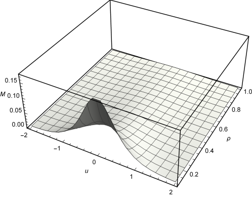
Figure 3: The gravitational COM density $M$ given by Eq. (43). The core of the wave burst is concentrated around $u=0$. The gravitational COM is similarly more intense around $u=0$, and vanishes when $\rho\rightarrow\infty$ and $u\rightarrow\pm\infty$. Therefore it is related to the localization of the wave burst.

As in Ref. [16], we see that the radial gravitational acceleration of a geodesic particle in space-time, given on the right hand side of Eq. (26) for the wave determined by Eq. (21), is negative and therefore directed towards the region with higher intensity of the gravitational centre of mass density, which plays the role of “centre of gravity”. The propagation of the gravitational wave may also be thought as the propagation in space-time of the COM density shown in Figure 3. Had we considered the plus sign in Eq. (21), the radial acceleration would be repulsive, with a minus sign multiplying the right hand side of Eq. (26), and also the right hand side of Eqs. (41-43) would be multiplied by $-1$.

5 Oscillating pp-wave

In this section we will consider the interesting case of an oscillating pp-wave. We will just multiply the Gaussian function by a harmonic function in the expression of $H(u,\rho)$, and again in this case the work-energy relation is verified. Let us consider the function

$$H=-\frac{1}{2}\ln{(\rho)}\cos{(u)}e^{-(u/10)^{2}}\,,$$ (44)

in the frame defined by Eqs. (7-8). The resulting inertial accelerations are

$$\phi_{(0)(1)} = \frac{\cos{\phi}\cos{u}}{4\rho\left(2-H\right)}e^{-(u/10)^{2}}=\phi_{(1)(3)}\,,$$ (45)

$$\phi_{(0)(2)} = \frac{\sin{\phi}\cos{u}}{4\rho\left(2-H\right)}e^{-(u/10)^{2}}=\phi_{(2)(3)}\,,$$ (46)

$$\phi_{(0)(3)} = -\frac{\left(\frac{u\cos{u}}{50}+\sin{u}\right)\ln{\rho}}{4\left(2-H\right)^{3/2}}e^{-(u/10)^{2}}\,.$$ (47)

As before, the gravitational acceleration on the frame is exactly minus the expressions above. In vector form, the gravitational acceleration is written as

$${\bf{a}}_{g} = -\frac{\cos{u}}{4\rho\left(2-H\right)}e^{-(u/10)^{2}}\hat{\rho}+\frac{\left(\frac{u\cos{u}}{50}+\sin{u}\right)\ln{\rho}}{4\left(2-H\right)^{3/2}}e^{-(u/10)^{2}}\hat{z}$$ (48)

$$\equiv a_{g\rho}\hat{\rho}+a_{gz}\hat{z}\,.$$

This is the acceleration of the particles that are hit by the wave.

The radial and longitudinal components of the gravitational acceleration above are displayed in Figures 4 and 5, respectively.

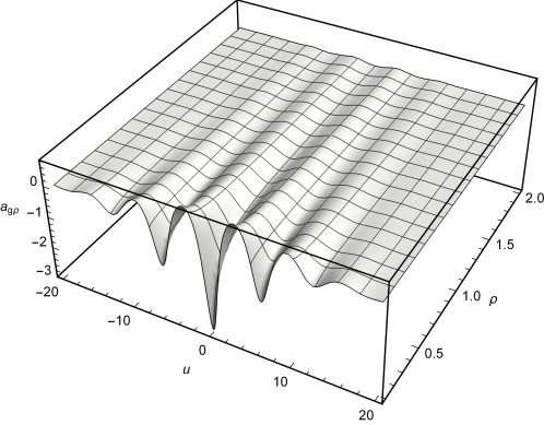
Figure 4: Radial gravitational acceleration for $H$ given by (44).

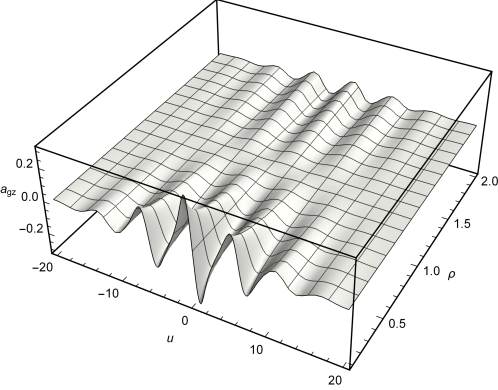
Figure 5: Longitudinal gravitational acceleration for $H$ given by (44).

The variations of the longitudinal acceleration, as given in Figure 5, suggests a trapping of a particle, but only along the $z$ direction. To some extent, this feature is similar to the trapping of particles discussed in Ref. [4].

We also analyse the distribution of the COM density for the oscillating wave. The non-vanishing components of the COM density are

$$-M^{(0)(1)} = \frac{k\cos{u}}{\sqrt{2}A^{3}}\frac{\cos{\phi}}{\rho}e^{-(u/10)^{2}}\,,$$ (49)

$$-M^{(0)(2)} = \frac{k\cos{u}}{\sqrt{2}A^{3}}\frac{\sin{\phi}}{\rho}e^{-(u/10)^{2}}\,,$$ (50)

where $A=\sqrt{2-H}$. In vector form, we have

$${\bf{M}}=\frac{k\cos{u}}{\sqrt{2}A^{3}}\;\frac{1}{\rho}\;e^{-(u/10)^{2}}\hat{\rho}\equiv M\hat{\rho}\,.$$ (51)

In Figure 6 we plot the quantity $M$ defined above with respect to both $u$ and $\rho$. Regions with higher, positive values of $M$ are attractive. It is interesting to note that Figures 4 and 6 are very much similar, except that one is inverted with respect to the other, and the same feature takes place in the former case of a non-oscillating wave. We see a relationship between the radial acceleration $a_{\rho}$ and the quantity $M$ defined by Eq. (51), which is given by

$$a_{\rho}=-(4\sqrt{2}\pi\,A)\,M\,.$$ (52)

Thus, if $M>0$, then $a_{\rho}$ is attractive. This feature justifies the consideration of the COM density of the waves. There is a not yet totally understood relationship between the gravitational acceleration and the gravitational COM density, in general.

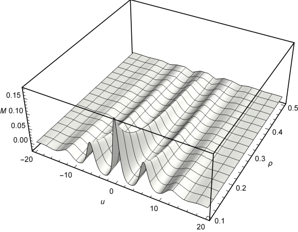
Figure 6: Centre of mass for $H$ given by (44).

Finally, we analyse the validity of the work-energy relation for particles on geodesics in the oscillating pp-wave determined by Eq. (44). Considering the initial conditions II, given by Eq. (35), where the initial condition $x(u_{0})=x_{0}$ may be varied, we find the results displayed in Figure 7.

Figure 7: $\Delta K$ (continuous line) and $\Delta W$ (dashed line) for the initial conditions II, and $H$ given by Eq. (44).

Once again, we verify that the work-energy relation is valid to an excellent approximation in the context of the oscillating pp-wave, which shows that the particles are indeed subject to the gravitational acceleration due to the wave.

6 Summary and conclusions

In this article we have considered the action on free particles of non-linear gravitational pp-waves, that propagate along the $z$ axis. The geodesic behaviour of these particles is such that before and after the passage of the wave, the particle trajectories are straight lines, i.e., they are free. We have carried out an attempt to explain why the final kinetic energy of particles may be smaller or larger than the initial values. The attempt is based on the classical work-kinetic energy relation of Newtonian physics $\Delta K=\Delta W$, where the work $\Delta W$ is given by Eq. (27), and $\Delta K$ by Eq. (30). Both $\Delta W$ and $\Delta K$ are quantities per unit mass. Figures 1, 2 and 7 show that the values of $\Delta W$ and $\Delta K$ are almost the same, by varying some of the initial conditions. That these two quantities are practically the same is a surprise, because $\Delta W$ is a relativistic quantity, whereas $\Delta K$ is clearly non relativistic. The difference between $\Delta W$ and $\Delta K$ may be due to this fact, as well as to some errors in the numerical (computer) evaluation of the quantities. In view of these results, we are led to define Eq. (27) as an exact, relativistic expression for the variation of the kinetic energy per unit mass $\Delta\textsf{K}$ of the particles. Thus, we define

$$\Delta\textsf{K}=\Delta W=-\int_{i}^{f}{\phi_{(0)(i)}e^{(i)}\,_{j}dx^{j}}\,,$$ (53)

for particles along geodesic trajectories. This expression is well defined as long as the notion of kinetic energy makes sense for geodesic particles. The equation above may be used to compute the variation of the kinetic energy of relativistic particles that travel at velocities close to the velocity of light, in the pp-wave space-times.

In the context of the gravitational waves considered in this article, there is an interesting relation between the radial acceleration $a_{\rho}$ and the intensity $M$ of the COM density. This relation is given by Eq. (52). Positive or negative values of $M$ imply attractive or repulsive radial gravitational acceleration, respectively. This relation will be investigated elsewhere, in the consideration of general gravitational field configurations.

One important conclusion of our analysis is that non-linear gravitational waves impart accelerations to particles that are hit by the wave. This acceleration, together with the initial conditions of the particle, lead to an increase or decrease of the energy of the particle, which implies, respectively, a decrease or increase of the gravitational energy of the wave, since the gravitational field is doing work on the particle. The quantity $\Delta W$ defined by Eqs. (27) and (53) determines the energy per unit mass that is exchanged between the particle and the gravitational wave. If the gravitational field does a positive work on the particle, the energy of the latter is increased, and a negative work implies $\Delta\textsf{K}<0$, exactly as in Newtonian mechanics. We expect Eq. (1) to be valid also for a charged particle if ${\bf a}$ is, in this case, the acceleration due to an electromagnetic wave, for instance. Therefore Eq. (1), understood as a generalised Torricelli equation, may have an universal character. It could be possible that the issues analysed in this article are also described in the context of the Newton-Cartan formulation of gravity.

References

- [1] P.-M. Zhang, C. Duval, G. W. Gibbons and P. A. Hovarthy, “The Memory Effect for Plane Gravitational Waves”, Phys. Lett. B 772, 743 (2017).
- [2] P.-M. Zhang, C. Duval, G. W. Gibbons and P. A. Hovarthy, “Soft gravitons and the memory effect for plane gravitational waves”, Phys. Rev. D 96, 064013 (2017).
- [3] P.-M. Zhang, C. Duval, G. W. Gibbons and P. A. Hovarthy, “Velocity Memory Effect for Polarized Gravitational Waves”, JCAP 05(2018)030.
- [4] P.-M. Zhang, M. Cariglia, C. Duval, M. Elbistan, G. W. Gibbons and P. A. Hovarthy, “Ion Traps and the Memory Effect for Periodic Gravitational Waves”, Phys. Rev. D 98, 044037 (2018).
- [5] K. Andrzejewski and S. Prencel, “Memory effect, conformal symmetry and gravitational plane waves”, Phys. Lett. B 782 (2018) 421.
- [6] Y. B. Zel´dovich and A. G. Polnarev, “Radiation of gravitational waves by a cluster of superdense stars”, Sov. Astron. 18, 17 (1974).
- [7] V. B. Braginsky and L. P. Grishchuk, “Kinematic resonance and memory effect in free-mass gravitational antennas”, Zh. Eksp. Teor. Fiz. 89, 744 (1985) [Sov. Phys. JETP 62, 427 (1985)].
- [8] R. Steinbauer, “Geodesics and geodesic deviation for impulsive gravitational waves”, J. Math. Phys. 39, 2201 (1998).
- [9] J. Podolský and K. Veselý, “New examples of sandwich gravitational waves and their impulsive limit”, Czech. J. Phys. 48, 871 (1998).
- [10] C. Sämann, R. Steinbauer and R. Švarc, “Completeness of general pp-waves spacetimes and their impulsive limit”, Class. Quantum Grav. 33, 215006 (2016).
- [11] J. Podolský, R. Švarc, R. Steinbauer and C. Sämann, “Penrose junction conditions extended: Impulsive waves with gyratons”, Phys. Rev. D 96 064043 (2017).
- [12] P.-M. Zhang, M. Elbistan, G. W. Gibbons and P. A. Hovarthy, “Sturm-Liouville and Carroll : at the heart of the Memory Effect”, Gen. Relativ. Grav. (2018) 50:107.
- [13] J. W. Maluf, J. F. da Rocha-Neto, S. C. Ulhoa and F. L. Carneiro, “Plane Gravitational Waves, the Kinetic Energy of Free Particles and the Memory Effect”, Gravitation and Cosmology 24, 216-266 (2018).
- [14] J. W. Maluf, J. F. da Rocha-Neto, S. C. Ulhoa and F. L. Carneiro, “Variations of the Energy of Free Particles in the pp-Wave Spacetimes”, Universe (2018), 4(7), 74.
- [15] J. W. Maluf, J. F. da Rocha-Neto, S. C. Ulhoa and F. L. Carneiro, “Kinetic Energy and Angular Momentum of Free Particles in the Gyratonic pp-Waves Space-times”, Class. Quantum Grav. 35, 115001 (2018).
- [16] J. W. Maluf, “The Teleparallel Equivalent of General Relativity and the Gravitational Centre of Mass”, Universe (2016), 2(3), 19.
- [17] J. Ehlers and W. Kundt, “Exact Solutions of the Gravitational Field Equations”, in “Gravitation: an Introduction to Current Research”, edited by L. Witten (Wiley, New York, 1962).
- [18] H. W. Brinkmann, “On Riemann spaces conformal to Euclidean spaces”, Proc. Natl. Acad. Sci. U.S. 9, 1 (1923); Math. Ann. 94, 119 (1925).
- [19] B. Mashhoon and U. Muench, “Length measurement in accelerated systems”, Ann. Phys. (Berlin) 11, 532 (2002).
- [20] B. Mashhoon, “Vacuum electrodynamics of accelerated systems: Nonlocal Maxwell’s equations”, Ann. Phys. (Berlin) 12, 586 (2003).
- [21] J. W. Maluf, F. F. Faria and S.C. Ulhoa, “On reference frames in spacetime and gravitational energy in freely falling frames”, Class. Quantum Grav. 24, 2743 (2007).
- [22] J. W. Maluf and F. F. Faria, “On the construction of Fermi-Walker transported frames”, Ann. Phys. (Berlin) 17, 326 (2008).
- [23] P. C. Aichelburg and R. U. Sexl, “On the gravitational field of a massless particle”, Gen. Relativ. Gravit. 2, 303 (1971).
- [24] C. Møller, “Tetrad Fields and Conservation Laws in General Relativity”, Proceedings of the International School of Physics “Enrico Fermi”, Edited by C. Møller (Academic Press, London, 1962).
- [25] J. W. Maluf, “The teleparallel equivalent of general relativity”, Ann. Phys. (Berlin) 525, 339-357 (2013).
- [26] J. W. Maluf, S. C. Ulhoa, F. F. Faria and J. F. da Rocha-Neto, “The angular momentum of the gravitational field and the Poincaré group”, Class. Quantum Grav. 23, 6245-6256 (2006).