Full Speed Ahead: 3D Spatial Database Acceleration with GPUs

Full Speed Ahead: 3D Spatial Database Acceleration with GPUs

Abstract

Many industries rely on visual insights to support decision-making processes in their businesses. In mining, the analysis of drills and geological shapes, represented as 3D geometries, is an important tool to assist geologists on the search for new ore deposits. Aeronautics manipulate high-resolution geometries when designing a new aircraft aided by the numerical simulation of aerodynamics. In common, these industries require scalable databases that compute spatial relationships and measurements so that decision making can be conducted without lags. However, as we show in this study, most database systems either lack support for handling 3D geometries or show poor performance when given a sheer volume of data to work with. This paper presents a pluggable acceleration engine for spatial database systems that can improve the performance of spatial operations by more than 3000x through GPU offloading. We focus on the design and evaluation of our plug-in for the PostgreSQL database system.

1 Introduction

Database systems are a fundamental component of software architectures that deal with the storage and retrieval of digital information. They are used on a variety of scenarios that include the management of large-scale datasets, data curation, and analysis. Data can be represented as a collection of tables that are manipulated through relational operators (as in the traditional relational database systems) or as unstructured documents that are accessed without a rigid schema, as seen in key-value or graph-based NoSQL databases.

As database systems offer generic interfaces to manage a large set of data types, it is expected that custom support for special classes of data may be missing, incomplete, or poorly implemented. One example of such a class is geospatial data; with a few exceptions, database systems are not readily able to distinguish geometries from other binary blobs nor to provide operators to enable filtering based on spatial properties and relationships between geometry types.

The geospatial services industry is estimated to have an economic impact at USD 1.6 trillion anually in revenues. The technology enables companies to sharpen decision making and save time and money [1]. Given the importance that geospatial data plays, several databases provide extensions to enable their base systems to handle spatial data types. That is the case of MySQL (with MySQL Spatial Extension, supporting 2D geometries), IBM’s DB2 (with its Spatial Extender for 2D data), PostgreSQL (that enables operations on 2D and 3D geometries through the PostGIS extension), and Oracle Database (that does the same with its Oracle Spatial extension) [2]. In common, such extensions enable the representation of geometries as if they were native data types (i.e., integer, floating point, text) and include a data model, new indexing methods, predicate functions, and topology operations, among others [3].

Despite the presence of spatial data types on modern databases, processing of 3D spatial queries often suffer from poor scalability on such platforms. The issue arises from a combination of an intensive demand for computational resources with the presence of very large collections of 3D objects. As a consequence, individual query evaluations can take several hours to complete or – worse – end up timing out and giving no results back to the user [4]. Such limitations severely restrict the applications of 3D spatial analysis supported by traditional database systems.

We present in this paper the design and evaluation of a database-agnostic accelerator for 3D spatial queries that removes the scalability problems aforementioned. Our prototype features specialized GPU kernels that perform spatial operations on geometries comprising millions of polygons and on a virtually unlimited number of objects. Our evaluation of the platform, based on a comparison with the open source PostGIS spatial extension to PostgreSQL, shows performance gains of more than 3000$\times$ on several use cases. We also describe a connector for PostgreSQL that enables the routing of queries over PostGIS functions and objects to our platform.

The paper is organized as follows. Section 2 gives an overview of database extensions that handle spatial data types and that enable access to foreign services. Next, Section 3 presents the core architecture of our accelerator. Section 4 compares the performance of our platform against CPU-based implementations. We present related work in Section 5 and make closing remarks thereafter in Section 6.

2 Database Extensions

The work described in this paper is based on two particular standards that have been incorporated into PostgreSQL. This section describes their purpose and how they relate to us.

2.1 Foreign Data Wrappers

A part of the SQL standard known as SQL/MED offers syntax extensions to SQL that enable access to data that lives outside the database through the table interface. There are no restrictions on where the foreign data must be stored: it can live on another database, on a remote filesystem, inside a structured file, or in any other repository determined by the user – as long as the remote server can handle the SQL/MED protocol and map the data to a tabular layout.

The SQL/MED interfaces allow a SQL server to receive a query that contains mixed references to local and remote tables. In that case, the SQL server decomposes the query into multiple fragments and dispatches them to the foreign servers as needed. It also devises and initiates an execution plan for each fragment, receives the responses from each remote server, and returns the result to the application [5].

Our acceleration platform implements a subset of the SQL/MED protocol that enables its integration with a regular database system. The data it exposes to the SQL server mirrors the original tables containing geometry data types, with a few restrictions. First, the mirror is populated on demand from the original SQL server. Second, the mirrored data is kept in memory in a format that can be readily parsed by the GPU kernels. Third, the only members from the original table that are mirrored are (i) the geometry data and (ii) its unique identifier; all operations involving other table members such as numerical or textual ones are processed by the SQL server itself. These decisions allowed us to focus on the spatial aspects of our engine with no need to implement a full featured database management system.

2.2 Spatial Data Types

There exist two major standards supporting the inclusion of spatial data types and operators into SQL databases. The first, SQL/MM (ISO/IEC 13249), extends SQL to address simple 2D elements and 3D geometries. It supports the management of collections of points, curves, surfaces, and a combination of primitives and spatial methods involving geometry sets [3]. The second standard is OGC Simple Feature Access, defined by the Open Geospatial Consortium. It supports the storage, retrieval, query and updates of feature collections in 2 or 3 spatial dimensions [6].

Our accelerator prototype supports a subset of the OGC standard: it handles geometries represented by points, triangulated irregular networks (TINs), polyhedral surfaces, and line strings. Three spatial operators are currently implemented: 3D Intersection, 3D Distance, and 3D Volume. Together, they cover the majority of the use cases whose performance we intend to improve.

3 Accelerating Spatial Databases

Here we describe the architecture of our platform, including its coupling with a SQL database system, and the algorithms we implemented to enable the efficient processing of selected spatial operations on GPUs.

3.1 Architecture

The acceleration platform implements a subset of the PostgreSQL protocol that handles user authentication, the execution of simple queries and prepared statements (including support for JOIN expressions and nested selections), and the retrieval of results through named cursors and anonymous portals. It can be accessed via regular PostgreSQL tools or through foreign data facilities.

An overview of our architecture is given in Figure 1. Two major components are shown: an instance of PostgreSQL, holding a table with a geometry and its attributes, and an instance of the GPU accelerator. The latter mirrors the geometry and its unique identifier from PostgreSQL; other table members are not carried over. Queries submitted to the PostgreSQL server are split according to the presence of foreign elements. On the depicted example, the non-spatial element of the query is handled directed by the PostgreSQL server, whereas the ST_Volume operation on the geometry column executes on the GPU accelerator.

The accelerator platform retrieves the geometry data from the original table and persists that data in system memory. This process is conducted asynchronously either on demand (as queries arrive) or at startup time. All data featured on the geometry column is processed by the GPUs, even in the presence of “WHERE” clauses that could restrict the computation to a smaller geometry set. We do so to prevent sub-optimal use of cores within the GPU’s streaming multiprocessors and to cache results of computations that may be asked in the near future. Under this platform, SQL “WHERE” clauses, if given, execute on the CPU over the GPU kernel’s output. The results are consolidated by the PostgreSQL server once both sides have finished executing their jobs.

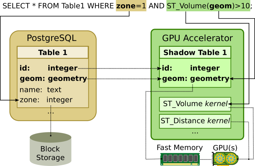
Figure 1: Queries are automatically split based on the presence of spatial operators. Regular operations are handled by the traditional PostgreSQL pipeline, whereas the spatial components are dispatched to our acceleration engine. The associated geometry data and identifiers are cached in memory and processed by specialized GPU kernels.

3.2 GPU Algorithms

In this section, we present how the volume, distance, and intersection algorithms are implemented on the GPU.

3.2.1 Volume

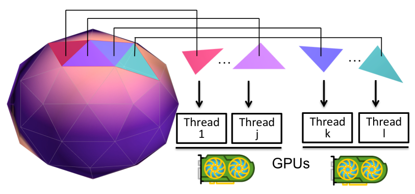
Figure 2: Example on how to evaluate the volume of a 3D triangle meshes using GPUs. According to the divergence theorem, it is possible to calculate the volume of a given solid mesh by using the normal of each face. Each GPU thread computes the area and the normal of each mesh triangle and these results are combined to compute the mesh volume. Other operators like distance and intersection use a similar approach in the sense that each GPU thread performs some basic computation on a solid face.

The proposed GPU accelerator employs the divergence theorem [7] to evaluate the volume of a 3D mesh indirectly by using the information related to each polygon face. The theorem is defined as

$$\oiiint_{V}{(\nabla\cdot\mathbf{F})}dV=\oiint_{S}{(\mathbf{F}\cdot\mathbf{n})}dS,$$ (1)

where $V$ represents a volume in $\mathbb{R}^{3}$, $S$ is the boundary of V ($S=\partial V$), $\mathbf{F}$ is a continuously differentiable vector field (flux) defined on a neighborhood of $V$, and $\mathbf{n}$ is the unit normal pointing outward $S$.

Let $P$ be a polyhedron representing a database geometry given by a set of triangles $A_{i}$, $i=0,...,N-1$ with vertices $(u_{i},v_{i},w_{i})$. As all the faces are counter clockwise on $A_{i}$, the outer unit normal $n$ to $P$ on each face $A_{i}$ is $n_{i}=\hat{n}_{i}\div|\hat{n}_{i}|$ where $\hat{n}=(v_{i}-u_{i})\times(w_{i}-u_{i})$. Therefore, if we assume a flux $F=\vec{p}/3$ where $\vec{p}$ is a point on the surface of P, then the volume ($V$) of $P$ can be evaluated as

$$V =\int_{P}{1}dP=\int_{P}{(\nabla\cdot\vec{p}/3)}dP=\frac{1}{3}\int_{\partial P}(\vec{p}\cdot n)d{(\partial P)}$$ (2)

$$=\frac{1}{3}\sum_{i=0}^{N-1}\int_{A_{i}}(u_{i}\cdot n_{i})d{A_{i}}=\frac{1}{6}\sum_{i=0}^{N-1}u_{i}\cdot\hat{n}_{i},$$

where we exploit the fact that the area of $A_{i}$ is $|\hat{n}|/2$, and $\vec{p}\cdot n_{i}$ is constant over each $A_{i}$. Figure 2 presents the strategy to accelerate the volume calculation of 3D polyhedral meshes. Differently from a sequential CPU execution, GPU threads calculate $u_{i}\cdot\hat{n}_{i}$ for each face $A_{i}$ in parallel. Depending on the number of faces of the solid, its volume can be computed in a single GPU parallel execution. The implementations of distance and intersection operators follow a similar approach as each GPU thread performs a basic computation on the solid’s face.

3.2.2 Distance

The current implementation of 3D distance supports the following geometries: (i) line segment/line segment, (ii) line segment/polyhedral surface, and (iii) point/polyhedral surface. The following explanation is related to the distance between line segment and polyhedral surface; the other distance variations employ an analogous approach. In order to find the distance between a line segment and a polyhedral surface we find the distance between each triangular face of the polyhedron and the line segment. Similarly to the volume calculation, the distance of each face and the line is calculated in a parallel GPU thread. Then, the minimum distance is returned to the user.

We employ the approach suggested by [8, 9] to evaluate the distance between a triangle and a line segment. Assume a line segment with end points $P_{0}$ and $P_{1}$ with parametric representation $L(t)=P_{0}+t\vec{d}$, $0\leq t\leq 1$ where $\vec{d}=P_{0}-P_{1}$. Let a triangle with vertices $V_{0},V_{1},V_{2}$ be represented as $T(u,v)=V_{0}+u\vec{e_{0}}+v\vec{e_{1}}$ where $\vec{e_{0}}=V_{1}-V_{0}$, $\vec{e_{1}}=V_{2}-V_{0}$, $0\leq u,v\leq 1$, and $u+v\leq 1$. The minimum distance is computed by locating the values $u,v,t$ so that $T(u,v)$ is the triangle point closest to $L(t)$. We find $u,v,t$ that minimizes the squared-distance $Q(u,v,t)$ (Equation 3) from $T$ to $L$ to find the minimum distance from $L$ to each mesh triangle $A_{i}$.

$$Q(u,v,t)=|T(u,v)-L(t)|^{2}$$ (3)

3.2.3 Intersection

The intersection supports the same geometries and utilizes the same face decomposition approach as the 3D distance. Whenever polyhedral meshes are involved in the computation, the operator decomposes the intersection evaluation of each polyhedral face in a GPU thread. We employ a less computationally-intensive evaluation for intersection when compared to the distance operator.

For instance, for the line segment and polyhedral surface intersection, each GPU thread intersects the line segment with the plane containing the given triangular face, and then determines whether or not the intersection point is within the triangle [8]. In this case, we represent the triangle with vertices $V_{0}$, $V_{1}$, and $V_{2}$ as $T(u,v,w)=uV_{0}+vV_{1}+wV_{2}$ where $w=1-u-v$, $0\leq u,v\leq 1$, $u+v\leq 1$. The triple $(u,v,w)$ is known as barycentric coordinates of $T$ [9]. Assume also a line segment with points $P_{0}$ and $P_{1}$ and parametric representation $L(t)=P_{0}+t\vec{d}$, $0\leq t\leq 1$ where $\vec{d}=P_{0}-P_{1}$. Then the values for $t,u,$ and $v$ should be

$$\begin{bmatrix}t\\ u\\ v\\ \end{bmatrix}=\frac{1}{(\vec{d}\times e_{1})\cdot(e_{0})}\begin{bmatrix}((P-V_{0})\times e_{0})\cdot e_{1}\\ (\vec{d}\times e_{1})\cdot(P-V_{0})\\ ((P-V_{0})\times e_{0})\cdot\vec{d}\\ \end{bmatrix},$$ (4)

where $e_{0}=V_{1}-V_{0}$ and $e_{1}=V_{2}-V_{0}$. If $t$, $u$, and $v$ respect the aforementioned contraints, then $L$ intersects $T$.

4 Performance Evaluation

Use case: the query acceleration platform has been evaluated on a synthetic data set that represent features from the mining domain [10]. The data contains three object types: (i) line segments representing drill holes, (ii) closed meshes representing the locations and areas of ore bodies, and (iii) block models used for mineral resource estimation. We restrict our tests to a single ore shape comprising 500 faces and to 5 million drill holes. The queries we run represent spatial operations that geologists perform on a daily basis: computing the volume of geological shapes, filtering drill holes based on their distance to profitable areas of a mine, and retrieving drill holes that intersect with certain objects of interest (such as a particular rock type).

Computing environment: our experiments were run on a bare metal machine with an Intel E5-2620 v4 featuring 16 cores, 256 GB of memory, 800 GB of SSD, and a NVIDIA Tesla V100 GPU. The software stack includes PostgreSQL 10.4 and PostGIS 2.4.4 with the SFCGAL backend (version 1.3.2) to enable the ST_Volume operator. Our GPU kernels were built with the Cuda compiler version 9.1.85. The PostgreSQL server and our accelerator were hosted on that same machine. Kernel page caches are flushed prior to each execution.

PostgreSQL settings: we changed the default amount of memory dedicated for caching data from 80 MB to 50 GB, enforced the use of parallel processing, configured the cost of non-sequentially-fetched disk pages to 1, and modified the estimated cost of the PostGIS functions to enable their execution with a varying number of workers.

Results: we separate the results in three sets: volume, distance, and intersection. Figure 3 shows the processing time to determine the distance of line segments to a 3D solid. PostGIS shows a significant variation, especially when few geometries are processed, due to cache hits in PostgreSQL buffers. We also note similar processing times with 16 and 32 CPUs. That is caused by PostgreSQL’ parallel planner, which picked 11 workers regardless of having enough geometries to keep all cores busy. Performance gains with pure CPU parallelization were of 6$\times$ when processing the full dataset. Our GPU-based accelerator, on the other hand, shows a consistent performance independently of how many geometries are asked by the user (1, 10, or 5 million): 0.685 seconds with a variation of 0.002 seconds. That is an improvement of 1860$\times$ over the sequential version of PostGIS.

For the intersection test, shown in Figure 4, we considered the 5 million segments case alone. The performance notes above regarding PostGIS apply again. This time, however, our GPU-based accelerator improves 3230$\times$ over PostGIS’ sequential run. As observed in Section 3.2.3, we employ a less computationally intensive algorithm for 3D intersection when compared to 3D distance, which leads to the dramatic speedup observed here.

We also computed the 3D volume of the same solid used on the other tests. PostGIS does not split the geometry among different workers, so a single processor is used at all times. PostGIS computes the volume in 2530 seconds, with a variation of 68 seconds. Since our GPU algorithm processes different faces on dedicated GPU processors, we observed a gain of 2770$\times$ at 0.91 seconds with a variation of 0.006.

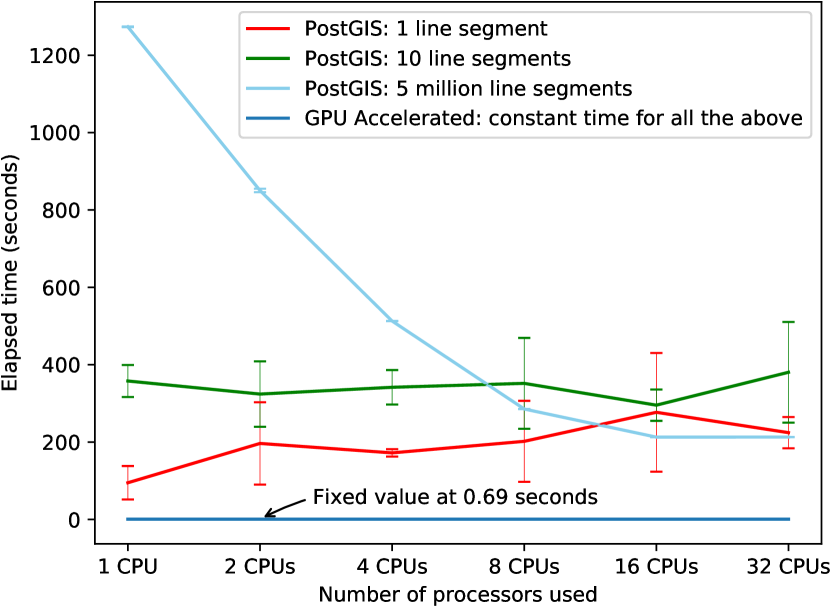
Figure 3: Variable performance of 3D distance computation on the CPU versus a constant time with our GPU accelerator.

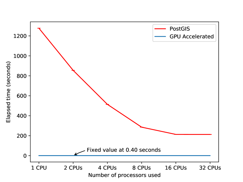
Figure 4: Performance of computing the 3D distance of 5 million line segments and a solid on the CPU and the GPU.

5 Related Work

Several areas of computation (e.g., artificial intelligence) are leveraging the vast amount of processing power and memory bandwidth provided by modern GPUs for data-intensive applications.

Recently, database researchers also employed GPUs for accelerating data management systems. In [11], the authors present a survey for GPU-accelerated database systems and argue that modern database management systems should be an in-memory, column-oriented using a block-at-a-time processing model, possibly extended by a just-in-time-compilation component. These systems also should have a query optimizer that is aware of co-processors (e.g. GPUs) and data-locality. An important problem in query optimization is join-order optimization. Current join-order optimizers employ dynamic programming in a sequential approach. In [12], the authors propose different ways to employ GPU-accelerated dynamic programming for join-order optimization, and discuss the challenges of this approach. Sitaridi et. al. propose an implementation of relational operators on GPU processors. Their focus is related to string matching in SQL queries. As GPU threads in the presence of different execution paths are serialized, they split string matching into multiple steps to reduce thread divergence. Their solution optimizes string search by selecting a given parallelism granularity and string layout for different algorithms.

6 Conclusions

The work presented in this paper shows that it is possible to obtain expressive performance gains from spatial queries (by more than 3000$\times$) by coupling existing database systems with a standalone accelerator supported by GPUs. As we conducted this work we identified several research opportunities, including geometry caching strategies, GPU-assisted data compression, pre-fetching algorithms, and cooperation between concurrent GPU kernels. We intend to investigate each of these topics in the near future.

References

- [1] A. Datta, “Where is the money in geospatial industry?” 2016, https://www.geospatialworld.net/article/where-is-the-money (visited on Jun 6, 2018).
- [2] A. Piórkowski, “MySQL Spatial and PostGIS - Implementations of Spatial Data Standards,” in Electronic journal of Polish agricultural universities, vol. 14, 01 2011, p. 03.
- [3] K. Stolze, “SQL/MM Spatial: The Standard to Manage Spatial Data in Relational Database Systems,” in Proceeding of the 10th Conference on Database Systems for Business, Technology, and Web (BTW), 2003, pp. 247–264.
- [4] S. Zhang, J. Han, Z. Liu, K. Wang, and S. Feng, “Spatial Queries Evaluation with MapReduce,” in 2009 Eighth International Conference on Grid and Cooperative Computing, Aug 2009, pp. 287–292.
- [5] J. Melton, J. E. Michels, V. Josifovski, K. Kulkarni, and P. Schwarz, “SQL/MED: A Status Report,” SIGMOD Rec., vol. 31, no. 3, pp. 81–89, Sep. 2002. [Online]. Available: http://doi.acm.org/10.1145/601858.601877
- [6] R. Chen and J. Xie, Open Source Databases and Their Spatial Extensions. Berlin, Heidelberg: Springer Berlin Heidelberg, 2008, pp. 105–129. [Online]. Available: https://doi.org/10.1007/978-3-540-74831-1_6
- [7] C. Gold, Spatial Context: An Introduction to Fundamental Computer Algorithms for Spatial Analysis, ser. ISPRS Book Series. CRC Press, 2018.
- [8] D. Eberly, 3D Game Engine Design: A Practical Approach to Real-Time Computer Graphics, ser. Morgan Kaufmann series in interactive 3D technology. Taylor & Francis, 2007.
- [9] P. Schneider and D. Eberly, Geometric Tools for Computer Graphics, ser. The Morgan Kaufmann Series in Computer Graphics. Elsevier Science, 2002.
- [10] K. Maestrini, “Synthetic dataset representing mine features,” http://lucasvr.gobolinux.org/publications/2018-ADMS-Dataset.zip (visited on Jul 22, 2018) .
- [11] S. Breß, M. Heimel, N. Siegmund, L. Bellatreche, and G. Saake, GPU-Accelerated Database Systems: Survey and Open Challenges. Berlin, Heidelberg: Springer Berlin Heidelberg, 2014, pp. 1–35. [Online]. Available: https://doi.org/10.1007/978-3-662-45761-0_1
- [12] A. Meister and G. Saake, “Challenges for a GPU-Accelerated Dynamic Programming Approach for Join-Order Optimization.” in In Proc. GI-Workshop GvDB, 2016, pp. 81–86.