Cost-efficient Data Acquisition on Online Data Marketplaces for Correlation Analysis

Abstract

Incentivized by the enormous economic profits, the data marketplace platform has been proliferated recently. In this paper, we consider the data marketplace setting where a data shopper would like to buy data instances from the data marketplace for correlation analysis of certain attributes. We assume that the data in the marketplace is dirty and not free. The goal is to find the data instances from a large number of datasets in the marketplace whose join result not only is of high-quality and rich join informativeness, but also delivers the best correlation between the requested attributes. To achieve this goal, we design DANCE, a middleware that provides the desired data acquisition service. DANCE consists of two phases: (1) In the off-line phase, it constructs a two-layer join graph from samples. The join graph consists of the information of the datasets in the marketplace at both schema and instance levels; (2) In the online phase, it searches for the data instances that satisfy the constraints of data quality, budget, and join informativeness, while maximize the correlation of source and target attribute sets. We prove that the complexity of the search problem is NP-hard, and design a heuristic algorithm based on Markov chain Monte Carlo (MCMC). Experiment results on two benchmark datasets demonstrate the efficiency and effectiveness of our heuristic data acquisition algorithm.

1 Introduction

With the explosion in the profits from analyzing the data, data has been recognized as a valuable commodity. Recent research [4] predicts that the sales of big data and analytics will reach $187 billion by 2019. Incentivized by the enormous economic profits, the data marketplace model was proposed recently [6]. In this model, data is considered as asset for purchase and sale. Many established companies (e.g. Twitter and Facebook), sell rich, structured (relational) datasets. But such datasets are often prohibitively expensive. Data marketplaces in the cloud enable to sell the (cheaper) data by providing Web platforms for buying and selling data; examples include Microsoft Azure Marketplace [3] and BDEX [1].

Age	Zipcode	Population
[35, 40]	10003	7,000
[20, 25]	01002	3,500
[55, 60]	07003	1,200
[35, 40]	07003	5,800
[35, 40]	07304	2,000

(a) $D_{S}$: Source instance owned by data shopper Adam

Zipcode State 07003 NJ correct 07304 NJ correct 10001 NY correct 10001 NJ wrong State Disease # of cases MA Flu 300 NJ Flu 400 Florida Lyme disease 130 California Lyme disease 40 NJ Lyme disease 200 $D_{1}$: Zipcode table $D_{2}$: Data and statistics of diseases by state (FD: Zipcode $\rightarrow$ State)

Gender Race Disease # of cases M White Flu 200 F Asian AIDS 30 M White Diabetes 4,000 M Hispanic Flu 140 Age Gender Race Population [35,40] M White 400,000 [20,25] F Asian 100,000 [20,25] M White 300,000 [40,45] M Hispanic 50,000 $D_{3}$: Data and statistics of diseases $D_{4}$: Census dataset of New Jersey (NJ) State of New Jersey (NJ) State by gender

Age Address Insurance Disease [35, 40] 10 North St. UnitedHealthCare Flu [20, 25] 5 Main St. MedLife HIV [35, 40] 25 South St. UnitedHealthCare Flu

$D_{5}$: Insurance & disease data instance

(b) Relevant instances on data marketplace

Table 1: An example of data acquisition

In this paper, we consider the data shopper who has a particular type of data analytics needs as correlation analysis of some certain attributes. He may own a subset of these attributes already. He intends to purchase more attributes from the data marketplace to perform the correlation analysis. However, many existing cloud-based data marketplaces (e.g., Microsoft Azure Marketplace [3] and Google Big Query service [2]) do not support efficient exploration of datasets of interest. The data shopper has to identify the relevant data instances through a non-trivial data search process. First, he identifies which datasets are potentially useful for correlation analysis based on the (brief) description of the datasets provided by the data marketplaces, which normally stays at schema level. There may exist multiple datasets that appear relevant. This leads to multiple purchase options. Based on these options, second, the shopper has to decide which purchase option is the best (i.e., it returns the maximum correlation of the requested attributes) under his constraints (e.g., data purchase budget). Let us consider the following example for more details.

Example 1.1.

Consider the data shopper Adam, a data research scientist, who has a hypothesis regarding the correlation between age groups and diseases in New Jersey (NJ), USA. Adam only has the information of age, zipcode, and population in his own dataset $D_{S}$ (Table 1 (a)). To test his hypothesis, Adam plans to purchase additional data from the marketplace. Assume that he identifies five instances $D_{1}$ - $D_{5}$ (Table 1 (b)) in the data marketplace as relevant. There are several data purchase options. Five of these options are listed below:

• Option 1: Purchase $D_{1}$ and $D_{2}$;

• Option 2: Purchase three attributes (Gender, Disease, # of cases) of $D_{3}$ and (Age, Gender, Population) of $D_{4}$;

• Option 3: Purchase three attributes (Race, Disease, # of cases) of $D_{3}$ and (Age, Race, Population) of $D_{4}$;

• Option 4: Purchase $D_{5}$;

• Option 5: Purchase $D_{1}$, $D_{2}$, $D_{3}$, and $D_{4}$.

For each option, the correlation analysis is performed on the join result of the purchased datasets and the data shopper’s local data (optional). In general, the number of possible join paths is exponential to the number of datasets in the data marketplaces. The brute-force method that enumerates all join paths to find the one that delivers the best correlation between a set of attributes is prohibitively expensive. Besides the scalability issue, there are several important issues for data purchase on the data marketplace. Next, we discuss them briefly.

Meaningful joins. Different joins return different amounts of useful information. For example, consider Option 1 and 2 in Example 1.1. Both Option 1 and 2 enable to generate the association between age and disease, but the join result in Option 1 is grouped by zipcode, while that of Option 2 is grouped by gender. Both join results are considered as meaningful, depending on how the shopper will test his hypothesis on the join results. On the other hand, the join result of Option 4 also includes the attributes Age and Disease. However, the join result is meaningless, as it associates the aggregation data with individual records.

Data quality. The data on the data marketplaces tends to be dirty (e.g., missing and inconsistent data values) [11]. In this paper, we consider data consistency as the main data quality issue. Intuitively, the data quality (in terms of its consistency) is measured as the percentage of data content that is consistent with a set of specific integrity constraints which take the form of functional dependency (FD) [9, 7]. For example, $D_{1}$ in Table 1 (b) has a FD: Zipcode $\rightarrow$ State (i.e., all the same Zipcode values must be associated with the same State value). However, the last record is inconsistent with the FD. Naturally, the shopper prefers to purchase the data with the highest quality (i.e., lowest inconsistency). Intuitively, there exists the trade-off between data quality and the performance of correlation analysis - purchasing more data may bring more insights for correlation analysis, but it may lead to more errors. A naive solution is to clean the data in the marketplace first; the purchase requests are processed on the cleaned data. However, we will show that data join indeed impacts the data quality significantly. The join of high-quality (low-quality, resp.) data instances can become low-quality (high-quality, resp.) in terms of data inconsistency. Therefore, data quality issue has to be dealt with online during data acquisition.

Data price and budget-constrained purchase. Data on the marketplaces are not free. We assume the data shopper is equipped with a limited budget for data purchase. Therefore, we follow the query-based pricing model [6] for the data marketplaces: a data shopper submits SQL queries to the data marketplaces and pays for the query results. This pricing model is also used by some cloud-based data marketplaces, e.g., Google Big Query service [2]. This pricing model supports the data shopper to purchase the necessary data pieces (e.g., purchase three attributes {Gender, Disease, # of cases} of $D_{3}$) instead of the whole dataset.

The issues of data scalability, data quality, join informativeness and the budget constraints make the data purchase from the data marketplaces extremely challenging for the data shoppers, especially for those common users who do not have much experience and expertise in data management. The existing works on data exploration [32, 22, 21] mainly focus on finding the best join paths among multiple datasets in terms of join size and/or informativeness. However, these solutions cannot be easily adapted to the setting of data marketplaces, due to the following reasons. First, it is too expensive to construct the schema graph [22] for all the data on the marketplace due to its large scale. Second, the search criteria for join path is different. While the existing works on data exploration try to find the join path of the best informativeness, our work aims to find the best join path that maximizes the correlation of a set of specific attributes, with the presence of the constraints such as data quality and budgets.

Contributions. We design a middleware service named DANCE, a Data Acquisition framework on oNline data market for CorrElation analysis, that provides cost-efficient data acquisition service for the budget-conscious search of the high-quality data on the data marketplaces that maximizes the correlation of certain attributes. DANCE consists of two phases: (1) during the off-line phase, it constructs a two-layer join graph of the datasets on the data marketplace. The join graph contains the information of these datasets at both schema and instance level. To deal with the data scalability issue of the marketplaces, DANCE collects samples from the data marketplaces, and constructs the join graph from the samples; (2) during the online phase, it accepts the data shoppers’ correlation request as well as the constraints (budgets, data quality, and join informativeness). By leveraging the join graph, it estimates the correlation of a certain set of attributes, as well as the join informativeness and quality of the data pieces to be purchased. Based on these estimated information, DANCE recommends the data pieces on the data marketplace that obtain the best correlation while satisfy the given constraints. In particular, We make the following contributions.

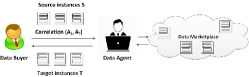
Figure 1: Framework of DANCE

First, we design a new sampling method named correlated re-sampling to deal with multi-table joins of large intermediate join size. We show how to unbiasedly estimate the correlation, join informativeness, and quality based on the samples.

Second, we design a new two-layer join graph structure. The join graph is constructed from the samples collected from the data marketplace. It includes the join relationship of the data instances at schema level, as well as the information of correlation, join informativeness, quality, and price of the data at instance level.

Based on the join graph, third, we transform the data acquisition problem to a graph search problem, which searches for the optimal subgraph in the join graph that maximizes the (estimated) correlation between source and target nodes, while the quality, join informativeness (in format of edge weights in the graph), and price satisfy the specified constraints. We prove that the problem of searching for such optimal subgraph is NP-hard. Thus, we design a heuristic algorithm based on Markov chain Monte Carlo (MCMC). Our heuristic algorithm first searches for the minimal weighted graph at the instance layer of the join graph, which corresponds to a set of specific instances. Then it finds the optimal target graph at the attribute set layer of the join graph, which corresponds to the attributes in those instances that are to be purchased from the marketplace.

Last but not least, we perform an extensive set of experiments on large-scale benchmark datasets. The result show that our search method can find the acquisition results with high correlation efficiently.

The rest of the paper is organized as following. Section 2 introduces the preliminaries. Section 3 presents the data sampling method. Section 4 and Section 5 present the off-line and online phase of DANCE respectively. Section 6 shows the experiment results. Section 7 discusses the related work. Section 8 concludes the paper.

2 Preliminaries

2.1 System Overview

We consider a data marketplace $\mathbf{M}$ that stores and maintains a collection of relational database instances $\mathcal{D}$ = $\{D_{1},\\ \dots,D_{n}\}$. A data shopper may own a set of relational data instances $\mathbb{S}$ locally, which contain a set of source attributes $\mathcal{A_{S}}$. The data shopper would like to purchase a set of target attributes $\mathcal{A_{T}}$ from $\mathbf{M}$, so that the correlation between $\mathcal{A_{S}}$ and $\mathcal{A_{T}}$ is maximized. In this paper, we only consider vertical purchase, i.e., the shopper buys the attributes from the data marketplaces. We assume the data shopper fully trusts DANCE. Figure 1 illustrates the framework of DANCE. DANCE consists of two phases: the offline and online phases.

Offline phase. During the offline phase, DANCE collects a set of samples from $\mathbf{M}$, and constructs a data structure named join graph that includes: (1) the join relationship among the samples at schema level; and (2) the information of correlation, join informativeness, quality, and price at instance level. Due to the high complexity of calculating the exact correlation, data quality, and join informativeness from the join results, the correlation, quality, and join informativeness are estimated from the collected samples.

Online phase. During the online phase, DANCE accepts the acquisition requests from data shoppers. Each acquisition request consists of: (1) the source dataset $\mathbb{S}$ that is owned by the shopper and the source attributes $\mathcal{A_{S}}\in\mathbb{S}$; (2) the target attributes $\mathcal{A_{T}}\in\mathcal{D}$, and (3) the budget $B$ of data purchase from $\mathbf{M}$, to DANCE. The data shopper can also specify his requirement of data quality and join informativeness by the setup of the corresponding threshold values. Both $\mathbb{S}$ and $\mathcal{A_{S}}$ are optional. The acquisition without $\mathbb{S}$ and $\mathcal{A_{S}}$ aims to find the best correlation of $\mathcal{A_{T}}$ in $\mathcal{D}$.

After DANCE receives the acquisition request, it first processes the request on its local join graph by searching for a set of target instances $\mathbb{T}=\{T_{1},\dots,T_{k}\}$, where: (1) for each $T_{i}$, there exists an instance $D_{j}\in\mathcal{D}$ such that $T_{i}\subseteq D_{j}$; (2) the correlation between $\mathcal{A_{S}}$ and $\mathcal{A_{T}}$ is maximized in $\mathcal{J}=\bowtie_{\forall T_{i}\in\mathbb{S}\cup\mathbb{T}}T_{i}$, where $\bowtie$ denotes the equi-join operator; (3) each $T_{i}\in\mathbb{T}$ is assigned a price, which is decided by a query-based pricing function [6]. The total price of $\mathbb{T}$ should not exceed $B$; and (4) the quality and join informativeness of $\mathcal{J}$ are beyond the threshold specified by the data shopper. If no such target instance can be identified from its current join graph and data samples, DANCE purchases more samples from $\mathbf{M}$, updates its local join graph, and performs the data search again. The iterative process continues until either the desired $\mathbb{T}$ is found or the data shopper changes his acquisition requirement (e.g., by relaxing the data quality threshold). The data shopper pays DANCE for the sample purchase during acquisition.

After DANCE identifies the target instances $\mathbb{T}$, it generates a set of SQL projection queries $\mathcal{Q}$, where each instance $T_{i}\in\mathbb{T}$ corresponds to a query $\mathsf{Q}\in\mathcal{Q}$. Each $\mathsf{Q}\in\mathcal{Q}$, denoted as $\pi_{A_{i}}(D_{i})$ $(\pi:$ the projection operator), selects a set of attributes $A_{i}$ from the instance $D_{i}$. We call the attribute set $A_{i}$ the projection attribute set. In the paper, we use $D.A$ to specify the values of attribute $A$ of the instance $D$.

After receiving the purchase option $\mathcal{Q}$ from DANCE, the data shopper sends $\mathcal{Q}$ to $\mathbf{M}$ directly, and obtains the corresponding instances.

2.2 Data Quality

In this paper, we consider the setting where data on the marketplaces is dirty. In this project, we mainly consider one specific type of dirty data, the inconsistent data, i.e., the data items that violate integrity constraints [5, 23]. A large number of existing works (e.g., [9, 7]) specify the data consistency in the format of functional dependency ($FD$). Formally, given a relational dataset $D$, a set of attributes $Y$ of $D$ is said to be functionally dependent on another set of attributes $X$ of $D$ (denoted $X\rightarrow Y$) if and only if for any pair of records $r_{1},r_{2}$ in $D$, if $r_{1}[X]=r_{2}[X]$, then $r_{1}[Y]=r_{2}[Y]$. For any FD $F:X\rightarrow Y$ where $Y$ contains multiple attributes, $F$ can be decomposed in to multiple FD rules $F^{\prime}:X\rightarrow Y^{\prime}$, with $Y^{\prime}$ containing a single attribute of $Y$. Thus for the following discussions, we only consider FDs that contain a single attribute at the right hand side.

Based on FDs, the data inconsistency can be measured as the amounts of data that does not satisfy the FDs. Before we formally define the measurement of data inconsistency, first, we formally define partitions. We use $r.A$ to denote the value of attribute $A$ of record $r$.

Definition 2.1

[Equivalence Class ($EC$) and Partitions] [12] The equivalence class ($EC$) of a tuple $r$ with respect to an attribute set $X$, denoted as $eq_{X}^{r}$, is defined as $eq_{X}^{r}=\{r^{\prime}|r.A=r^{\prime}.A,\forall A\in X,\forall r^{\prime}\in D\}$. The set $\pi_{X}=\{eq_{X}^{r}|r\in D\}$ is defined as a partition of $D$ of the attribute set $X$. Informally, $\pi_{X}$ is a collection of disjoint sets ($ECs$) of tuples, such that each set has a unique representative value of the set of attributes $X$, and the union of the sets equals $D$.

Given a dataset $D$ and an FD $F:X\rightarrow Y$, where $X$ and $Y$ are a set of attributes, the degree of data inconsistency by $F$ can be measured by the fraction of records that do not satisfy FDs. Following this, we define the data quality function $Q(D,F)$ for a given FD $F$ on an instance $D$.

Definition 2.2

[Data quality of one instance w.r.t. one FD] Given a data instance $D$ and a FD $F:X\rightarrow Y$ on $D$, for any equivalence class $eq_{x}\in\pi_{X}$, the correct equivalence class in $\pi_{X\cup Y}$ is

$$C(D,X\rightarrow Y,eq_{x})= \{eq_{xy}|eq_{xy}\in\pi_{X\cup Y},eq_{xy}\subseteq eq_{x},$$ (1)

$$\nexists eq^{\prime}_{xy}\in\pi_{X\cup Y}\text{ }s.t.\text{ }eq^{\prime}_{xy}\subseteq eq_{x}\text{ and }$$

$$|eq_{xy}^{\prime}|>|eq_{xy}|\}.$$

In other words, $C(D,X\rightarrow Y,eq_{x})$ is the largest equivalence class in $\pi_{XY}$ with the same value on $X$ attributes as $eq_{x}$. If there are multiple such equivalence classes of the same size, we break the tie randomly.

Based on the definition of correct equivalence classes, the set of correct records in $D$ w.r.t. $F$ is defined as:

$$C(D,X\rightarrow Y)=\bigcup_{eq_{x}\in\pi_{X}}C(D,X\rightarrow Y,eq_{x}).$$ (2)

The quality of a given data instance $D$ w.r.t. $F:X\rightarrow Y$ is measured as:

$$Q(D,X\rightarrow Y)=\frac{|C(D,X\rightarrow Y)|}{|D|},$$ (3)

TID	A	B
$t_{1}$	$a_{1}$	$b_{1}$
$t_{2}$	$a_{1}$	$b_{1}$
$t_{3}$	$a_{1}$	$b_{2}$
$t_{4}$	$a_{1}$	$b_{3}$
$t_{5}$	$a_{2}$	$b_{2}$

Table 2: An example of data instance $D$ ($FD:A\rightarrow B$)

Example 2.1.

Consider the data instance $D$ in Table 2 and the FD $A\rightarrow B$ on $D$. The partition $\pi_{A}$ on $A$ consists of two equivalence classes, $eq_{A}^{a_{1}}=\{t_{1},t_{2},t_{3},t_{4}\}$ and $eq_{A}^{a_{2}}=\{t_{5}\}$. The partition $\pi_{AB}$ consists of four equivalence classes, i.e., $eq_{AB}^{a_{1},b_{1}}=\{t_{1},t_{2}\}$, $eq_{AB}^{a_{1},b_{2}}=\{t_{3}\}$, $eq_{AB}^{a_{1},b_{3}}=\{t_{4}\}$, and $eq_{AB}^{a_{2},b_{2}}=\{t_{5}\}$. Then $C(D,A\rightarrow B,eq_{A}^{a_{1}})=eq_{AB}^{a_{1},b_{1}}$, while $C(D,A\rightarrow B,eq_{A}^{a_{2}})=eq_{AB}^{a_{2},b_{2}}$. Therefore, the set of correct tuples is $C(D,A\rightarrow B)=\{t_{1},t_{2},t_{5}\}$. The tuples $t_{3}$ and $t_{4}$ are considered as error.

As we consider the dirty datasets that may be inconsistent, the exact FDs may not hold on those dirty datasets. Instead we consider approximate functional dependencies (AFDs) which allow FDs to hold on the data with small errors. Formally, an AFD $F$ holds on the dataset $D$ if $Q(D,F)\geq\theta$, where $\theta\in(0,1)$ is a user-defined threshold value. Based on the definition of AFDs, now we are ready to define the quality of a set of instances.

Definition 2.3

[Data quality] Given a set of instances $\mathcal{D}$, let $\mathcal{J}$ = $\bowtie_{\forall D_{i}\in\mathcal{D}}D_{i}$, and $\mathcal{F}$ be the set of AFDs hold on $\mathcal{J}$. The set of correct records of $D$ w.r.t. $\mathcal{F}$ are defined as $C(\mathcal{J},\mathcal{F})=\bigcap_{\forall F_{i}\in\mathcal{F}}C(\mathcal{J},F_{i})$, where $C(\mathcal{J},F_{i})$ follows Equation (2). The quality of $\mathcal{D}$ w.r.t. $\mathcal{F}$ is measured as

$$Q(\mathcal{D})=\frac{|C(\mathcal{J},\mathcal{F})|}{|\mathcal{J}|},$$ (4)

Intuitively, the quality is measured as the portion of the records that are correct among all the FDs on the instance.

Impact of Join on Data Quality. To provide high-quality data for purchase, a naive solution is to clean the inconsistent data off-line before processing any data acquisition request online. However, this solution in incorrect, since join can change data quality. High-quality datasets may become low-quality after join, and vice versa. Example 2.2 shows an example.

TID	A	B	C
$t_{1}$	$a_{1}$	$b_{1}$	$c_{4}$
$t_{2}$	$a_{1}$	$b_{1}$	$c_{5}$
⋮	⋮	⋮	⋮
$t_{996}$	$a_{1}$	$b_{1}$	$c_{999}$
$t_{997}$	$a_{1}$	$b_{2}$	$c_{1}$
$t_{998}$	$a_{1}$	$b_{2}$	$c_{2}$
$t_{999}$	$a_{1}$	$b_{3}$	$c_{3}$
$t_{1000}$	$a_{1}$	$b_{3}$	$c_{3}$

(a) $D_{1}:A\rightarrow B$ ($Q(D_{1})=0.996$)

TID C D E $t_{1}$ $c_{1}$ $d_{1}$ $e_{1}$ $t_{2}$ $c_{1}$ $d_{1}$ $e_{1}$ $t_{3}$ $c_{2}$ $d_{1}$ $e_{2}$ $t_{4}$ $c_{3}$ $d_{1}$ $e_{2}$ $t_{5}$ $c_{4}$ $d_{1}$ $e_{2}$	TID A B C D E $t_{1}$ $a_{1}$ $b_{2}$ $c_{1}$ $d_{1}$ $e_{1}$ $t_{2}$ $a_{1}$ $b_{2}$ $c_{1}$ $d_{1}$ $e_{1}$ $t_{3}$ $a_{1}$ $b_{2}$ $c_{2}$ $d_{1}$ $e_{2}$ $t_{4}$ $a_{1}$ $b_{3}$ $c_{3}$ $d_{1}$ $e_{2}$ $t_{5}$ $a_{1}$ $b_{3}$ $c_{3}$ $d_{1}$ $e_{2}$
(b) $D_{2}:D\rightarrow E$	(c) $D_{1}\Join D_{2}$: $A\rightarrow B$, $D\rightarrow E$
$Q(D_{2})=0.6$	$Q(D_{1}\Join D_{2})=0.2$

Table 3: An example that the join of two high-quality data instances is low-quality

Example 2.2.

In Table 3 (a) and (b), we display two datasets with good quality. The correct records in $D_{1}$ include $\{t_{1},t_{2},\dots,t_{996}\}$. Thus $Q(D_{1})=0.996$. Similarly, the correct records in $D_{2}$ include $\{t_{3},t_{4},t_{5}\}$. Thus $Q(D_{2})=0.6$. After the join of $D_{1}$ and $D_{2}$ (the join result is shown in Table 3 (c)), there only exist 5 tuples. We get $C(D_{1}\Join D_{2},A\rightarrow B)=eq_{(a_{1},b_{2})}=\{t_{1},t_{2},t_{3}\}$, while $C(D_{1}\Join D_{2},D\rightarrow E)=eq_{(d_{1},e_{2})}=\{t_{3},t_{4},t_{5}\}$. Therefore, $Q(D_{1}\Join D_{2})=0.2$.

Example 2.2 shows that performing data cleaning before join is not acceptable. The data quality has to be measured on the join result.

2.3 Join Informativeness

Evaluating whether the join result is informative simply by join size is not suitable. For example, consider the join of $D_{S}$ and $D_{5}$ in Table 1. The join is meaningless since it associates the aggregation data with individual records. But its join size is larger than the other options (e.g., join $D_{S}$ with $D_{1}$) that are more meaningful. Therefore, we follow the information-theory measures in [33] to quantify how informative the join is. Given two attribute sets $X$ and $Y$, let $I(X,Y)$ and $H(X,Y)$ denote the mutual information and entropy of the joint distribution $(X,Y)$ respectively. The join informativeness is formally defined below.

Definition 2.4

[Join Informativeness [33]] Given two instances $D$ and $D^{\prime}$, let $J$ be their join attribute(s). The join informativeness of $D$ and $D^{\prime}$ is defined as

$$JI(D,D^{\prime})=\frac{H(D.J,D^{\prime}.J)-I(D.J,D^{\prime}.J)}{H(D.J,D^{\prime}.J)},$$ (5)

by using the joint distribution of $D.J$ and $D^{\prime}.J$ in the output of the full outer join of $D$ and $D^{\prime}$.

The reason of using the outer join for the join informativeness measurement is to deal with values in $D$ and $D^{\prime}$ that do not match, i.e., pairs of type (val, NULL). The informativeness function penalizes those joins with excessive numbers of such unmatched values [31]. The join informativeness value always falls in the range [0, 1]. It is worth noting that the smaller $JI(D,D^{\prime},J)$ is, the more important is the join connection between $D$ and $D^{\prime}$.

2.4 Correlation Measurement

Quite a few correlation measurement functions (e.g. Pearson correlation coefficient , token inverted correlation [25], and cross correlation (autocorrelation)) can evaluate the correlation of multiple attributes. However, they can deal with either categorical or numerical data, but not both. Therefore, we use the Shannon entropy based correlation measure [20] to quantify the correlation as it deals with both categorical and numerical data.

Definition 2.5

[Correlation [20]] Given a dataset $D$ and two attribute sets $X$ and $Y$, the correlation of $X$ and $Y$ $CORR(X,Y)$ is measured as

• $CORR(X,Y)=H(X)-H(X|Y)$ if $X$ is categorical,

• $CORR(X,Y)=h(X)-h(X|Y)$ if $X$ is numerical,

where $H(X)$ is the Shannon entropy of $X$ in $D$, and $H(X|Y)$ is the conditional entropy:

$$H(X|Y)=\sum H(X|y)p(y),$$

Furthermore, $h(X)$ is the cumulative entropy of attribute $X$

$$h(X)=-\int P(X\leq x)logP(X\leq x)dx,$$

and

$$h(X|Y)=-\int h(X|y)p(y)dy.$$

2.5 Problem Definition

Intuitively, the data shopper prefers to purchase the high-quality, affordable data instances that can deliver good join informativeness, and most importantly, the best correlation. We assume the data samples have been obtained from the data marketplace. Formally, given a set of data samples $\mathcal{D}=\{D_{1},\dots,D_{n}\}$ collected from the data marketplace, a set of source instances $\mathbb{S}$ with source attributes $\mathcal{A_{S}}$, a set of target attributes $\mathcal{A_{T}}$, and the budget $B$ for data purchase, the data acquisition problem is defined as the following: find a set of database instances $\mathbb{T}\subseteq\mathcal{D}$ such that

$$\underset{\mathbb{T}}{\text{maximize}} CORR(\mathcal{A_{S}},\mathcal{A_{T}})$$

subject to $$\forall T_{i}\in\mathbb{T},\exists D_{j}\in\mathcal{D}\ s.t.\ T_{i}\subseteq D_{j},$$

$$\sum_{T_{i}\in\mathbb{S}\cup\mathbb{T}}JI(T_{i},T_{i+1})\leq\alpha,$$

$$Q(\mathbb{T})\geq\beta,$$

$$p(\mathbb{T})\leq B,$$

where $\alpha$ and $\beta$ are the user-specified thresholds for join informativeness and quality respectively. We note that $CORR(\mathcal{A_{S}},\mathcal{A_{T}})$ is measured on the join result. We assume that the data shopper can be guided to specify appropriate parameter values for $\alpha$ and $\beta$. The output $\mathbb{T}$ will guide DANCE to suggest the data shopper of the SQL queries for data purchase from the data marketplaces.

3 Data Sampling and Estimation

In this section, we discuss how to estimate join informativeness, data quality, and correlation based on samples. We use the correlated sampling [30] method to generate the samples from the data marketplace. General speaking, for any tuple $t_{i}\in D_{1}$, let $t_{i}[J]$ be its join attribute value. The record $t_{i}$ is included in the sample $S_{1}$ if $h(t_{i}[J])\leq p_{1}$, where $h()$ is the hash function that maps the join attribute values uniformly into the range $[0,1]$, and $p_{1}$ is the sampling rate. The sample $S_{2}$ of $D_{2}$ is generated in the same fashion.

3.1 Estimation of Join Informativeness

For a pair of data instances $D_{1}$ and $D_{2}$, let $S_{1}$ and $S_{2}$ be the samples of $D_{1}$ and $D_{2}$ by using correlated sampling. Then the join informativeness $JI(D_{1},D_{2})$ is estimated as:

$$\hat{JI}(D_{1},D_{2})=JI(S_{1},S_{2}),$$ (6)

where $JI()$ follows Equation (5).

Next, we have Theorem 3.1 to show that the estimated join informativeness is unbiased and is expected to be accurate.

Theorem 3.1.

Let $D_{1}$ and $D_{2}$ be two data instances, and $S_{1}$ and $S_{2}$ be the sampled dataset by using correlated sampling with the same sampling rate. It must be true that the expected value of the estimated join informativeness $E(JI(S_{1},S_{2}))$ satisfies that:

$$E(JI(S_{1},S_{2}))=JI(D_{1},D_{2}).$$

We present the proof of Theorem 3.1 in our full paper [17].

3.2 Correlated Re-sampling for Estimation of Correlation & Quality

One weakness of the correlated sampling for estimation of the correlation and data quality is that the size of join result from samples can be extremely large, especially for the join of a large number of data instances. Note that this is not a problem for estimation of join informativeness as it only deals with 2-table joins. To deal with the large join result, we design the correlated re-sampling method by adding a second-round sampling of the join results. Intuitively, given a set of data instances $(D_{1},\dots,D_{p})$, for any intermediate join result $IJ$, if its size exceeds a user-specified threshold $\eta$, we sample$IJ^{\prime}$ from $IJ$ by using a fixed re-sampling rate, and use $IJ^{\prime}$ for the following joins. In this way, the size of the intermediate join result is bounded.

For the sake of simplicity, for now we only focus on the re-sampling of 3-table joins (i.e., $D_{1}\Join D_{2}\Join D_{3}$). Let $S_{1}$, $S_{2}$ and $S_{3}$ be the samples of $D_{1}$, $D_{2}$, and $D_{3}$ respectively. Let $S_{12}^{\prime}$ denote the re-sampling result of $S_{1}\Join S_{2}$ if its size exceeds $\eta$, or $S_{1}\Join S_{2}$ otherwise. The estimated correlation and quality are

$$\widehat{CORR}_{D_{1}\Join D_{2}\Join D_{3}}(\mathcal{A_{S}},\mathcal{A_{T}})=CORR_{S_{1,2}^{\prime}\Join S_{3}}(\mathcal{A_{S}},\mathcal{A_{T}}),$$ (7)

$$\hat{Q}(D_{1},D_{2},D_{3})=Q(S_{1,2}^{\prime},S_{3}).$$ (8)

The estimation can be easily extended to the join paths of arbitrary length, by applying sampling on the intermediate join results. Next, we show that the correlation and data quality estimation by using correlated re-sampling is also unbiased.

Theorem 3.2.

Given a join path $(D_{1},D_{2},D_{3})$, let $S_{1,2}^{\prime}$ be the sample from $S_{1}\Join S_{2}$. It must be true that the expected value of the estimated correlation $E(CORR_{S_{1,2}^{\prime}\Join S_{3}})$ satisfies:

$$E(CORR_{S_{1,2}^{\prime}\Join S_{3}}(\mathcal{A_{S}},\mathcal{A_{T}}))=CORR_{D_{1}\Join D_{2}\Join D_{3}}(\mathcal{A_{S}},\mathcal{A_{T}}),$$

and the expected value of the estimated quality $E(Q({S_{1,2}^{\prime},S_{3}}))$ satisfies:

$$E(Q({S_{1,2}^{\prime},S_{3}}))=Q(D_{1},D_{2},D_{3}),$$

where $\mathcal{A_{S}}$ and $\mathcal{A_{T}}$ are the source and target attribute sets that are included in $D_{1}$ and $D_{3}$.

Due to the space limit, we show the proof of Theorem 3.2 in our full paper [17]. We must note that the estimation is unbiased regardless of the value of $\eta$.

4 Off-line Phase: Construction of Join Graph

In this section, we present the concept of join graph, the main data structure that will be used for our search algorithm (Section 5). First, we define the attribute set lattice of a single data instance.

Definition 4.1

[Attribute Set Lattice (AS-lattice)] Given a data instance $D$ that has $m$ attributes $\mathcal{A}$, it corresponds to an attribute set lattice (AS-lattice) $\mathcal{L}$, in which each vertex corresponds to a unique attribute set $\mathcal{A}^{\prime}\subseteq\mathcal{A}$. For the vertex $v\in\mathcal{L}$ whose corresponding attribute set is $\mathcal{A}^{\prime}$, it corresponds to the projection instance $\pi_{\mathcal{A^{\prime}}}(D)$. Given two lattice vertice $L_{1},L_{2}$ of $\mathcal{L}$, $L_{2}$ is $L_{1}$’s child (and linked by an edge) if (1) $\mathcal{A}_{1}\subseteq\mathcal{A}_{2}$, and (2) $|\mathcal{A}_{2}|=|\mathcal{A}_{1}|+1$, where $\mathcal{A}_{1}$ and $\mathcal{A}_{2}$ are the corresponding attribute sets of $L_{1}$ and $L_{2}$. $L_{1}$ is an ancestor of $L_{2}$ (linked by a path in $\mathcal{L}$) if $\mathcal{A}_{1}\subset\mathcal{A}_{2}$. $L_{1}$ and $L_{2}$ are siblings if they are at the same level of $\mathcal{L}$.

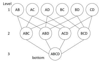
Figure 2: An example of attribute set lattice

Given $D$ and its $m$ attributes $\mathcal{A}$, the height of the attribute set lattice of $D$ is $m-1$. The bottom of the lattice contains a single vertex, which corresponds to $\mathcal{A}$, while the top of the lattice contains ${m}\choose{2}$ vertices, each corresponding to a unique 2-attribute set. Figure 2 shows an example of the attribute set lattice of an instance of four attributes $\{A,B,C,D\}$. In general, given an instance of $m$ attributes, its attribute set lattice consists of ${m}\choose{2}$ + $\dots$ + ${m}\choose{m}$ = $2^{m}-m-1$ vertices.

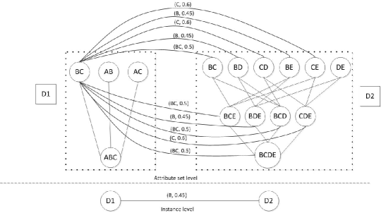
Figure 3: An example of a join graph for two instances $D_{1}(ABC)$ and $D_{2}(BCDE)$. Dotted rectangles represent tables. Only the node $BC$ of instance $D_{1}$ has all edges. The edges of other nodes are omitted for simplicity.

Next, we define join graph. In the following discussion, we use $\mathsf{AS}(v)$ to denote the attribute set that the vertex $v$ corresponds to.

Definition 4.2

[Join Graph] Given a set of data instances (samples) $\mathcal{D}=\{D_{1},\dots,D_{n}\}$, it corresponds to an undirected, weighted, two-layer join graph $G$:

• Instance layer (I-layer): each vertex at this layer, called instance vertex (I-vertex), represents a data instance $D_{i}\in\mathcal{D}$. There is an edge $e_{ij}$, called I-edge, between any two I-vertices $v_{i}$ and $v_{j}$ if $\mathsf{AS}(v_{i})\cap\mathsf{AS}(v_{j})\neq\emptyset$.

• Attribute set layer (AS-layer): for each I-vertex $v_{i}$, it projects to a set of vertices, called attribute set vertex (AS-vertex), at the AS-layer, each corresponding to an unique attribute set of the instance $D_{i}$. The AS-vertices that was projected by the same I-vertex construct the AS-lattice (Def. 4.1). Each AS-vertex $v_{i}$ is associated with a price $p_{i}$. For any two AS-vertices $v_{i}$ and $v_{j}$ that were projected by different I-vertices and $\mathsf{AS}(v_{i})\cap\mathsf{AS}(v_{j})\neq\emptyset$, there is an edge $e_{ij}$, called AS-edge, that connects $v_{i}$ and $v_{j}$. Each AS-edge is associated with a pair $(J,w_{i,j})$, where $J=\mathsf{AS}(v_{i})\cap\mathsf{AS}(v_{j})$, and the weight $w_{i,j}$ is the join informativeness of $D_{i}$ and $D_{j}$ on the join attributes $J$.

Definition 4.2 only specifies the weight of AS-edges. Next, we define the weight of I-edges. For any two I-vertices $v_{i}$ and $v_{j}$, let $AE$ be the set of AS-edges $\{(v_{k},v_{l})\}$ where $v_{k}$ ($v_{l}$, resp.) is an AS-vertex that $v_{i}$ ($v_{j}$, resp.) projects to. The weight of the I-edge $(v_{i},v_{j})$ is defined as the $w_{i,j}=\min_{(v_{k},v_{l})\in AE}w(k,l)$.

The I-layer can be constructed from the schema information of datasets in the marketplaces. Many existing marketplace platforms (e.g., [3, 2]) provide such schema information. AS-layer will be constructed from the data samples obtained from the marketplace. Intuitively, there exists the trade-off between accuracy and cost. More samples lead to more accurate estimation of join informativeness, quality, and correlation at the AS-layer. But this costs DANCE for purchase of samples.

Given a set of $n$ data instances $\mathcal{D}$ , its join graph contains $n$ instance vertices and $\Sigma_{i=1}^{n}(2^{m_{i}}-m_{i}-1)$ AS-vertices, where $m_{i}$ denotes the number of attributes in $D_{i}$. Figure 3 shows an example of the join graph. An important property of the join graph is that all the AS-edges that connect the AS-vertices in the same instances with the same join attributes always have the same weight (i.e., the same join informativeness). For instance, the edges ($D_{1}.AB$, $D_{2}.BC$) and ($D_{1}.BC$, $D_{2}.BD$) have the same weight. Formally,

Property 4.1

For any two AS-edges $(v_{i},v_{j})$ and $(v_{i}^{\prime},v_{j}^{\prime})$, if $v_{i}$ and $v_{i}^{\prime}$ were associated with the same I-vertex, as well as for $v_{j}$ and $v_{j}^{\prime}$, and $\mathsf{AS}(v_{i})\cap\mathsf{AS}(v_{j})=\mathsf{AS}(v_{i}^{\prime})\cap\mathsf{AS}(v_{j}^{\prime})$ (i.e., they have the same join attributes), then the two edges $(v_{i},v_{j})$ and $(v_{i}^{\prime},v_{j}^{\prime})$ are associated with the same weight.

Property 4.1 is straightforward by following the definition of the join informativeness. For example, consider the join graph in Figure 3, the edge $(D_{1}.BC,D_{2},BD)$ has the same weight as $(D_{1}.BC,D_{2},BDE)$, as well as $(D_{1}.AB,D_{2},BE)$ (not shown in Figure 3). Property 4.1 is in particular useful since it reduces the complexity of graph construction to exponential to the number of join attributes, instead of exponential to the number of all attributes. We will also make use of this property during graph search (Section 5) to speed up the search algorithm.

We must note that the join informativeness does not have the monotone property (i.e., the join on a set of attributes $J$ has higher/lower join informativeness than any subset $J^{\prime}\subset J$). As shown in Figure 3, the join informativeness (i.e., weight) of join attributes $BC$ is higher than that of join attribute $B$, but lower than that of the join attribute $C$.

Given a join graph, the source and target attributes $\mathcal{A_{S}}$ and $\mathcal{A_{T}}$ can be represented as special vertices in the join graph, formally defined below.

Target attribute set	Covered instance vertex
$\{AB\}$	$v_{1}$, $v_{2}$, $v_{3}$ (3 vertices)
$\{A\}$	$v_{1}$, $v_{2}$, $v_{3}$, $v_{4}$ (4 vertices)
$\{B\}$	$v_{1}$, $v_{2}$, $v_{3}$, $v_{5}$ (4 vertices)
$\{C\}$	$v_{5}$, $v_{6}$ (2 vertices)
$\{BC\}$	$v_{5}$, $v_{7}$ (2 vertices)

Table 4: An example of target vertex sets

Definition 4.3

[Source/target vertex sets] Given the source instances $\mathbb{S}$, the source attributes $\mathcal{A_{S}}$, and the target attributes $\mathcal{A_{T}}$, and a join graph $G$. An instance vertex $v\in G$ is a source I-vertex if its corresponding instance $D\in\mathbb{S}$. An instance vertex $v\in G$ is a target I-vertex if its corresponding instance $D$ is a source instance in $\mathbb{S}$ that contains at least one target attribute $A\in\mathcal{A_{T}}$. A set of AS-vertices $VS$ is a source (target, resp.) AS-vertex set if $\cup_{\forall v_{i}\in VS}\mathsf{AS}(v_{i})$ = $\mathcal{A_{S}}$ ($\mathcal{A_{T}}$, resp.). In other words, the AS-vertex set covers all source (target, resp.) attributes.

Since some attributes may appear in multiple instances, there exist multiple source/target AS-vertex sets. Example 4.1 shows an example of the possible target vertex sets.

Example 4.1.

Consider a set of target attributes $\mathcal{A_{T}}=\{A,B,C\}$. These target attributes can be covered by four different options:

• Option 1: they are covered by two instances, one containing {A, B} and the other containing {C};

• Option 2: they are covered by three instances, one containing {A}, the second containing {B}, and the third containing {C};

• Option 3: they are covered by two instances, one containing {A} and the other containing {B, C}; and

• Option 4: they are covered by two instances, one containing {A, B} and the other containing {B, C}.

Table 4 shows all possible target instance vertices. Following Table 4, there are 3$\times 2=6$ possible target AS-vertex sets for Option 1, 4$\times$ 4 $\times$ 2 = 32 target AS-vertex sets for Option 2, 4$\times$ 2 = 6 sets for Option 3, and 3$\times$ 2 = 6 sets for Option 4. Note that some of these target vertex sets are duplicates, e.g., $v_{5}^{BC}$ covers both attribute sets {C} and {B,C}. In total there are 43 unique target AS-vertex sets.

Based on the join graph and the source/target AS-vertex sets, the data acquisition problem is equivalent to finding a subgraph named target graph in the join graph, which corresponds to the instances for purchase. Next, we formally define the target graph.

Definition 4.4

[Target Graph] Given a join graph $G$, a set of source AS-vertex sets $\mathcal{SV}$, and a set of target AS-vertex sets $\mathcal{TV}$, a connected sub-graph $TG\subseteq G$ is a target graph if there exists a source AS-vertex set $SV\in\mathcal{SV}$ and a target AS-vertex set $TV\in\mathcal{TV}$ such that $TG$ contains both $SV$ and $TV$.

The target graph requires that it covers all source and target attributes. Next, we define the price, weight, and the quality of the target graph. Given a target graph $TG$, the price of $TG$ is defined as $p(TG)=\sum_{\forall_{v_{i}\in TG}}p_{i}$. The weight of $TG$ is defined as: $w(TG)=\sum_{\forall(v_{i},v_{j})\in TG}w(i,j)$. And the quality of $TG$, denoted as $Q(TG)$, is defined per Equation 4. Based on these definitions, now the data purchase problem can be mapped to the following graph search problem.

Problem statement Given a join graph $G$, a set of source AS-vertex sets $\mathcal{SV}$, a set of target AS-vertex sets $\mathcal{TV}$, and a budget $B$, find the optimal target graph (OTG) $G^{*}\subseteq G$ that satisfies the following constraint:

Maximize $$CORR(\mathcal{A_{S}},\mathcal{A_{T}})$$ (9)

Subject to $$w(G^{*})\leq\alpha,$$

$$Q(G^{*})\geq\beta,$$

$$p(G^{*})\leq B,$$

where $\alpha$ and $\beta$ are user-specified threshold for join informativeness and quality. We have the following theorem to show the complexity of the graph search problem.

Theorem 4.2.

The OTG search problem is NP-hard.

The proof of Theorem 4.2 can be found in our full paper [17].

5 Online Phase: Data Acquisition

Given the acquisition request $(\mathcal{A_{S}},\mathcal{A_{T}}$) with his source data $\mathbb{S}$, the brute-force approach is to search all possible target graphs in the join graph to find the best one (i.e., $\mathcal{A_{S}}$ and $\mathcal{A_{T}}$ have the largest correlation). Obviously this approach is not scalable, given the fact that there is a large number of data instances in the data marketplace, and each data instance has exponentially many choices of attribute sets. Therefore, we design a heuristic algorithm based on Markov chain Monte Carlo (MCMC) method. The intuition is that with fixed $(\mathcal{A_{S}},\mathcal{A_{T}})$, a large target AS-vertex set usually renders the join with small correlation and high join informativeness over longer join paths. Our algorithm consists of two steps. First, we find the minimal weighted I-layer graphs (I-graphs) (i.e., minimal join informativeness and thus higher correlation). The I-vertices in the subgraph correspond to the data instances. Second, we find the optimal target graph at the AS-layer (AS-graphs) from the minimal weighted I-graphs; the AS-vertices in the target graph correspond to the attribute sets of the instances identified by the first step. Next, we present the details of the two steps.

5.1 Step 1: Find Minimal Weighted Graphs (I-graphs) at I-layer

Given the source and target vertices, our graph search problem can be transformed to the classic Steiner tree problem that searches for a minimal tree that connects the source and target vertices. The Steiner tree problem is NP-hard. The complexity of the approximation algorithm [29] is quadratic to the number of nodes, which may not be acceptable for large graphs. In this paper, we design a heuristic algorithm whose complexity is logarithmic to the number of nodes in the graph. Our algorithm extends the approximate shortest path search algorithm [10]. The key idea is to randomly pick a set of I-vertices as the landmarks. For each I-vertex in $G$, our algorithm pre-computes and stores the shortest weighted paths to these landmarks, by using the shortest path search algorithm in [10]. Then given the source and target AS-vertex sets $\mathcal{A_{S}}$ and $\mathcal{A_{T}}$, for each landmark $v_{m}$, the algorithm constructs a graph by connecting each vertex in $\mathcal{A_{S}}\cup\mathcal{A_{T}}$ and $v_{m}$, via their shortest weighted paths. The output I-graph is constructed as the union of all the shortest weighted paths. If the total weight of the I-graph exceeds $\alpha$, there does not exist a target graph that satisfies the join informativeness constraint. Therefore, the algorithm returns no output. Due to space limit, we omit the pseudo code. It can be found in our full paper [17].

5.2 Step 2: Find Optimal Target Graphs (AS-graphs) at AS-layer

Input : A minimal weighted I-graph $\mathcal{IG}$

Output : A target graph $G^{*}$ at the AS-layer

1 $G^{*}=NULL$;

2 $Max=0$;

3 $TG=\mathcal{IG}$;

4 for $i=1$ to $\ell$ do

5      

6      Randomly pick an edge $e_{i,j}\in TG$;

7       Randomly pick a different edge $e^{\prime}_{i,j}$ between $(v_{i},v_{j})$;

8       Let $TG^{\prime}$ be the new target graph;

9       if $p(TG^{\prime})\leq B$ $\wedge$ $w(TG^{\prime})\leq\alpha$ $\wedge$ $Q(TG^{\prime})\geq\beta$ then

10             if accept $e^{\prime}_{i,j}$ by probability $\min(1,\frac{CORR(TG^{\prime})}{CORR(TG)})$ then

11                   $TG=TG^{\prime}$;

12                   if $CORR(TG)>Max$ then

13                         $G^{*}=TG$;

14                         $Max:=CORR(G^{*})$;

15                        

16                   end if

17                  

18             end if

19            

20       end if

21      

22 end for

23Return $G^{*}$;

Algorithm 1 FindJoinTree_AttSet(): find optimal target graph at attribute set layer

Based on the data instances selected by Step 1, Step 2 further selects the projection attributes of these instances by searching at the AS-layer of the minimal weighted I-graph. Algorithm 1 shows the pseudo code of Step 2. The key idea of Step 2 is to generate a sample of the graph at AS-layer iteratively by replacing the join attribute set of one edge $e_{i,j}$ with a different join attribute set. The algorithm runs $\ell$ iterations and keeps the sample of the largest correlation between the source and target vertices (Line 11 - 14). Some samples may not satisfy the constraints on weights, quality, and/or price. For each new sample, we first check if it satisfies these constraints (Line 8). After that, we use a Markov Chain Monte Carlo (MCMC) process to generate samples with high correlation, so as to maximize the utility of the output. In particular, for each graph, the algorithm randomly picks an edge $e_{i,j}$ (Line 5), which represents the join between two instances $D_{i}$ and $D_{j}$. From all the possible join attributes between $D_{i}$ and $D_{j}$, the algorithm randomly picks one, which corresponds to the AS-edge $e^{\prime}_{i,j}$, and replaces $e_{i,j}$ with $e^{\prime}_{i,j}$ by the acceptance probability $\min(1,\frac{CORR(TG^{\prime})}{CORR(TG)})$ (Line 9). Intuitively, the target graph of high correlation is accepted with high probability. During the iterations, the algorithm always keeps the graph sample that has the largest correlation between the source and target vertices, and return it after $\ell$ iterations.

5.3 Complexity Analysis

The complexity of Step 1 is $O(k(|\mathcal{A_{S}}|+|\mathcal{A_{T}}|)\log_{2}n)$, where $k$ is the average size of the minimal weighted graphs at the I-layer, and $n$ is the number of data samples on DANCE (i.e., the number of vertices at the I-layer of the join graph). In the experiments, we observe that $k$ is much smaller than $n$, especially when $n$ is large. The complexity of Step 2 is $O(\ell C_{J})$, where $\ell$ is the number of iterations, and $C_{J}$ is the average join cost of the instances in the I-graph returned by Step 1. Note that $C_{J}$ depends on both the size of I-graphs, and the size of each instance in the I-graph. The total complexity of the graph search algorithm is dominated by Step 2, which is $O(\ell C_{J})$.

	# of instances	Min. instance size	Max. instance size	Min. # of attributes	max. # of attributes	Avg # of FDs per table
		(# of records)	(# of records)
TPC-H	8	5 (Region)	6,000,000 (Lineitem)	4 (Region)	20 (Lineitem)	39
TPC-E	29	4 (Exchange)	10,001,048 (Watchitem)	3 (Sector)	28 (Customer)	33

Table 5: Dataset description

(a) $Q_{1}$	(b) $Q_{2}$	(c) $Q_{3}$

Figure 4: Time Performance w.r.t. various # of instances and join length (TPC-H dataset)

(a) Various # of instances

# of Instances	$Q_{1}$	$Q_{2}$	$Q_{3}$
10	3	5	5
15	7	4	7
20	5	4	4
25	5	4	6
29	3	5	8

(b) I-graph size

Budget Ratio	$Q_{1}$	$Q_{2}$	$Q_{3}$
0.04	3.067	N/A	N/A
0.06	6.487	30.62	N/A
0.08	7.478	49.23	766.8
0.10	7.478	51.43	980.9
0.12	7.478	51.43	1009.8

(c) Various budget ratio (N/A: not affordable)

’

Figure 5: Time performance w.r.t. various # of instances and budget ratios (TPC-E dataset)

Query	Approach	Correlation	Quality	Join Informativeness	Price
$Q_{1}$	With DANCE	12.51	0.07688	0.8906	60.65
	Purchase from data marketplace	18.18	0.3819	0.8268	63.12
$Q_{2}$	With DANCE	7.216	0.3968	1.248	59.78
	Purchase from data marketplace	7.965	0.4244	1.040	103.2
$Q_{3}$	With DANCE	3.609	0.08632	2.063	100.5
	Purchase from data marketplace	4.592	0.1026	2.104	106.4

Table 6: Comparison between data acquisition with DANCE and purchase from the data marketplace directly (TPC-H dataset, budget ratio=0.13)

6 Experiments

6.1 Experimental Setup

Implementation & Testbed. We implement the algorithms in Python. All the experiments are executed on a machine with 2 $\times$ Intel(R) Xeon(R) Silver 4116 CPU @ 2.10GHz, 12 cores, 24 processors, and 128 GB memory.

Datasets We use the TPC-E and TPC-H benchmark datasets in our experiments. The details of these two datasets are shown in Table 5. The tables that are of the minimum/maximum number of records are shown in a pair of parentheses. The longest join path in TPC-H and TPC-E datasets are of length 7 and 8 respectively.

Functional Dependency (FD) We measure the number of FDs on the TPC-E and TPC-H datasets. We use $\theta=0.1$ as the as the user-defined threshold for FDS (i.e. the amount of records that do not satisfy FDs is less than 10% of the dataset). We find that the number of FDs varies for each instance of TPC-H and TPC-E dataset. For example, there are 114 FDs in the LineItem table and 6 FDs in Region table in the TPC-H dataset.

Data quality. We modified 30% of records of 6 tables in TPC-H dataset (except region and Nation tables), and 20 out of 29 tables in TPC-E dataset to introduce inconsistency into the tables.

Data acquisition queries. In this section, we use the term target graph and join path interchangeably. For each dataset, we define three queries $Q_{1}$, $Q_{2}$ and $Q_{3}$ of short, medium, and long join paths respectively. In particular, for TPC-H dataset, $Q_{1}$, $Q_{2}$ and $Q_{3}$ are of join path length 2, 3, and 5, while for TPC-E dataset, $Q_{1}$, $Q_{2}$ and $Q_{3}$ are of join path length 3, 5, and 8.

Pricing model & budget. We use the entropy-based model for the data marketplace [16] to assign the price to data. To simulate the various budget settings, for each acquisition query, we pick the minimum and maximum price of all possible paths between source and target vertices as the lowerbound $LB$ and upperbound $UB$ of the total budget. We define the shopper’s budget as $r\times UB$, where $r\in(0,1]$ is the budget ratio. Intuitively, the larger $r$ is, the more budget that the shopper can purchase the data. We require that $r\times UB\geq LB$, i.e., the shopper can afford to purchase the instances of at least one target graph in the join graph.

Evaluation metric. To evaluate the performance of our sampling-based heuristic algorithm, we compare the correlation of the identified data instances by our algorithm and two optimal algorithms, namely the local optimal (LP) algorithm and the global optimal (GP) algorithm. Both LP and GP algorithms are the brute-force algorithms that enumerate all paths to find the one of the highest correlation. LP algorithm uses the samples as the input, and the GP algorithm uses the original datasets as the input. For all the algorithms, we measure the real correlation, not the estimated value. Let $X_{OPT}$ and $X$ be the correlation of the output by the (LP/GP) optimal approach and our heuristic approach respectively. The correlation difference of is measured as $CD=\frac{X_{OPT}-X}{X_{OPT}}$. Intuitively, the smaller correlation difference is, the more accurate our heuristic algorithm is.

6.2 Scalability

First, we measure the time performance of our heuristic algorithm with various number of data instances. In Figure 4, we compare the time performance of our heuristic algorithm against LP and GP on TPC-H data. First, we observe that our heuristic algorithm is significantly more efficient than the two optimal algorithms, especially when $n$ (the number of instances) is large. For example, when $n=8$, our heuristic algorithm can be 2,000 times more efficient than LP, and 20,000 times more efficient than GP. We are aware that for $Q_{3}$, the heuristic algorithm has comparable time performance to LP when $n=5$. This is because for this case, there is only a single I-graph that connects the source and target vertices, which lead to the same search space of our heuristic algorithm and LP. Second, we observe that the time performance of the heuristic algorithm is stable when the number of instances varies. Since the number of instances is small, the I-graph discovered by Step 1 (Section 5.1) remains the same. So does the search space of Step 2 (Section 5.2). Therefore, the time performance keeps stable. Third, we observe that the time of both LP and GP increase with the growth of $n$. This is not surprising since the number of I-graphs that connect the source and target vertices increase with the growth of $n$.

Figure 5 (a) and (b) show the time performance on TPC-E dataset. Since the two optimal algorithms do no halt within 10 hours on this large dataset, we only show the time performance of our heuristic algorithm in Figure 5 (a), and present the I-graph size (i.e., the number of vertices in the graph) for these settings in Figure 5 (b). An important observation is that the time performance does not increase with the growth of $n$. This is because when we vary the number of instances, the I-graph size indeed fluctuates considerably. However, we do observe that, in general, our heuristic algorithm takes more time when the I-graph is larger. For example, when the I-graph size is 8, it takes 1,010 seconds; while when the I-graph only includes 3 vertices, it can be as fast as 7.3 seconds.

(a) $Q_{1}$	(b) $Q_{2}$	(c) $Q_{3}$

Figure 6: Correlation difference w.r.t. various sampling rate (TPC-H dataset)

(a) $Q_{1}$	(b) $Q_{2}$	(c) $Q_{3}$

Figure 7: Correlation w.r.t. various budget ratio (TPC-H dataset)

(a) $Q_{1}$	(b) $Q_{2}$	(c) $Q_{3}$

Figure 8: Correlation with and without re-sampling w.r.t. various re-sampling rates (TPC-H dataset)

We also measure the time performance of our heuristic algorithm with regard to various budget ratios. Figure 5 (c) shows the time performance of our heuristic algorithm with various budget ratios on TPC-E dataset. We vary the budget ratio from 0.04 to 0.12, where 0.04 is the minimum budget ratio that can find at least one solution for either of the three queries $Q_{1}$, $Q_{2}$ and $Q_{3}$, while 0.12 is the highest budget ratio that can find at least one solution for all the three queries. With a small budget ratio, DANCE may not be able to find an affordable acquisition solution for some queries. For example, there is no acquisition solution for $Q_{3}$ when the budget ratio is under 0.06 (noted as N/A in Figure 5 (c)). From the results, first, we observe that DANCE takes more time when the budget ratio grows. However, the time performance may keep stable when the budget ratio is sufficiently large. For example, when the budget ratio is higher than 0.08, the time performance of $Q_{1}$ keeps unchanged. This is because with budget ratio 0.08, every target graph sample in Algorithm 1 becomes affordable. For this case, DANCE calculates the correlation of all the samples to find the one with the highest correlation. The number of samples keeps the same even if we increase the budget. Second, DANCE takes more time to process the acquisition requests of longer join paths. This is straightforward since it takes more time to join the instances in the longer path, and estimate the correlation and quality. We also measure the time performance on TPC-H dataset, and have similar observation as TPC-E dataset. Due to the space limit, we present the detailed results in our full paper [17].

6.3 Correlation

First, we measure the difference of the correlation of source and target attribute sets in the datasets returned by our heuristic algorithm and the two optimal algorithms with regard to various sampling rates. Intuitively, we want the correlation difference to be close to 0. The results are shown in Figure 6. First, we notice that the correlation difference is very small. In all cases, it never exceeds 0.31. Recall that in Figure 4, our heuristic algorithm can be 2,000 times more efficient than the optimal methods. This demonstrates that our method can efficiently find the datasets of correlation that is comparable to the optimal results. Second, we observe that the correlation difference decreases when the sampling rate grows. This is straightforward as more samples lead to more accurate correlation estimation.

Second, we measure the correlation between source and target attributes in the data acquisition result returned by our heuristic algorithm, as well as in the two optimal algorithms, on TPC-H dataset. The comparison results are displayed in Figure 7. First, we notice that the correlation by our heuristic algorithm is close to that of both optimal algorithms. In all cases, the difference is at most 5.9 (the maximum correlation is around 19). Second, with the increase of the budget ratio, the correlation in the results returned by all the three algorithms gradually rise (i.e., the correlation gets stronger). This is straightforward, as higher budget can afford to purchase more data with better utility. We do not show the correlation measurement results on TPC-E dataset, due to the long execution time of the GP algorithm.

We also measure the impacts of re-sampling on the correlation by changing the re-sampling rate and measuring the correlation of the acquisition result by our heuristic algorithm with and without re-sampling. The result is presented in Figure 8. We observe that the correlation with re-sampling oscillates around the correlation without re-sampling. The difference gradually reaches 0 with the growth of the re-sampling rate. Overall, the estimated correlation with re-sampling is accurate. The difference with the estimated correlation without re-sampling never exceeds 4.5.

6.4 Data Acquisition with DANCE vs. without DANCE

We compare the data acquisition results (correlation, data quality, join informativeness, and price) by DANCE with direct purchase from the data marketplace. We use GP algorithm to find the data acquisition results on the data marketplace. The comparison result is displayed in Table 6. First, we observe a large overlap between the data acquisition results returned by DANCE and GP. For instance, for $Q_{3}$, the data acquisition results returned by DANCE is {orders(totalprice, custkey), customer(custkey, H), supplier(H, nationkey), nation(nationkey, regionkey), region
(regionkey, rname)}, where H is one of the fake join attribute that is added to the data, while the results returned by GP is {orders(totalprice, custkey), customer(custkey, nationkey, H), supplier(nationkey, H), nation(nationkey, regionkey), region(regionkey, rname)}. Due to the space limit, we omit the target graph discovered by both approaches in Table 6. Second, we observe that the correlation of the data acquisition results returned by DANCE is comparable to that of GP. It can be as high as 90% of the optimal result. Third, the join informativeness of the data acquisition by both DANCE and GP is also close, which demonstrates the superiority of our correlated re-sampling method. The price of the data acquisition results returned by DANCE is always lower than that of GP. For example, it is 42% lower than the price of $Q_{2}$ on the data marketplace. This shows that DANCE is able to find the data of high utility (correlation) at a lower price. We acknowledge that in some cases, the quality of the data acquisition results returned by DANCE (e.g., $Q_{1}$) is significantly lower than that of GP, due to the error introduced by the sampling-based estimation. However, in most cases, the accuracy is still satisfying ($Q_{2}$ and $Q_{3}$).

7 Related Work

The concept of data market is firstly formally defined in [6]. Kanza et al. [13] envision a geo-social data marketplace that facilitates the generation and selling of high-quality spatio-temporal data from people. Koutris et al. [16] propose a query-based data pricing model for the market, considering the complicated queries that involve conjunctive sub-queries. The history-aware pricing model [28] avoids the buyer from getting charged repeatedly for the same data returned by different queries. Ren et al. [24] focus on the joint problem of data purchasing and data placement in a cloud data market. None of them studies the correlation-driven purchase on the data marketplace. The key to the data market model is the pricing model. Balazinska et al. [6] propose the data pricing model in which the buyers are charged based on the queries. A fundamental requirement named arbitrage-free requirement is identified in the pricing function, in order to prevent the buyers from intentionally reducing the charge by decomposing a complex query into multiple simple ones. QueryMarket [15] demonstrates the superiority of such a query-based data pricing model in real-world applications. Koutris et al. [16] prove that it is NP-complete to determine the arbitrage-free price of certain conjunctive selection queries for a given database instance. Lin et al. [18] study the arbitrage-free requirement theoretically and discover the sufficient conditions to enforce it in two models. The first model is instance-independent, in which the pricing function depends on the query only, and is irrelevant to the database instance. The other one is named the delayed model in which the price is determined by both the query and the result. Based on the findings of [18], Deep et al. [8] prove that any monotone, submodular and subadditive pricing function satisfies the arbitrage-free query pricing requirement. A survey of pricing models can be found in [19].

A relevant line of work is to explore the databases that contain complex database schemas via joins. Intuitively, given a database with schema graph, in which two tables are specified as the source and destination tables, the problem is to find a valid join path between the source and destination. To solve this problem, Procopiuc et al. [21] compute a probability for each join path that connects a given source table to a destination table. To speed up the exploration over the complex schema graph, Yang et al. [33] propose a new approach that summarizes the contents of a relational database as a summary graph. The most relevant tables and join joins can be computed from the summary graph. It defines the importance of each table in the database as its stable state value in a random walk over the schema graph, where the transition probability is defined based on the entropies of table attributes. Zhang et al. [34] take the reverse-engineering approach. In particular, given a database $D$ with schema graph $G$ and an output table $Out$, the problem is to compute a join query $Q$ that generates $Out$ from $D$. Unlike these work that mainly focus on the join informativeness of data instances, we take multiple factors, including join informativeness, data quality, and price, into consideration for the data marketplace.

Regarding the related work on subgraph search, the work on centerpiece subgraphs [27, 26], and on entity-relationship subgraphs [14] partially share with our goal: for a given set of query nodes and a budget constraint, output a connecting subgraph that meets the budget and maximizes some goodness measure. These works mainly focus on mining the patterns of some specific subgraphs, while we focus on finding the optimal subgraph with regards to the given constraints on informativeness, quality, and price.

8 Conclusion

In this paper, we study the data acquisition problem for correlation analysis in the data marketplace framework. We consider quality, join informativeness, and price issues of data acquisition, and model the data acquisition problem as a graph search problem. We prove that the graph search problem is NP-hard, and design a heuristic algorithm based on Markov chain Monte Carlo (MCMC). Our experiment results demonstrate the performance of our algorithm.

For the future, there are quite a few interesting research directions to explore. For example, instead of the best acquisition scheme, DANCE may recommend a number of acquisition options of the top-k scores to the data buyer, where the scores can be defined as a combination of correlation, data quality, join informativeness, and price. This raises the issues of how to define a fair score function, as well as the design of efficient top-k search algorithm when the score function is not be monotone. Additional issues that are worth to explore include how to deal with heterogeneous data in the marketplace, and how to deal with fast-evolving data in the data marketplace. Furthermore, an important issue is the privacy of the data marketplaces. In particular, when DANCE is not fully trusted, how can the data shopper exchange the information of the source instances with DANCE in a privacy-preserving way, and find correlated instances in the data marketplace? How to verify if the data in the marketplace is genuine (i.e., it is not fabricated)?

References

- [1] Bdex. http://www.bigdataexchange.com/.
- [2] Google bigquery data warehouse. https://cloud.google.com/bigquery/.
- [3] Microsoft azure data marketplace. https://azuremarketplace.microsoft.com/en-us/marketplace/?source=datamarket.
- [4] Idc’s worldwide semiannual big data and analytics spending guide taxonomy. http://www.informationweek.com/big-data/, 2016.
- [5] M. Arenas, L. Bertossi, and J. Chomicki. Consistent query answers in inconsistent databases. In Proceedings of the ACM Symposium on Principles of Database Systems, pages 68–79, 1999.
- [6] M. Balazinska, B. Howe, and D. Suciu. Data markets in the cloud: An opportunity for the database community. Proceedings of the VLDB Endowment, 4(12):1482–1485, 2011.
- [7] F. Chiang and R. J. Miller. Discovering data quality rules. Proceedings of the VLDB Endowment, 1(1):1166–1177, 2008.
- [8] S. Deep and P. Koutris. The design of arbitrage-free data pricing schemes. In International Conference on Database Theory, 2017.
- [9] W. Fan, F. Geerts, X. Jia, and A. Kementsietsidis. Conditional functional dependencies for capturing data inconsistencies. ACM Transactions on Database Systems, 33(2):6, 2008.
- [10] A. Gubichev, S. Bedathur, S. Seufert, and G. Weikum. Fast and accurate estimation of shortest paths in large graphs. In Proceedings of ACM International Conference on Information and Knowledge Management, pages 499–508, 2010.
- [11] P. N. Hague, N. Hague, and C.-A. Morgan. Market research in practice: How to get greater insight from your market. Kogan Page Publishers, 2013.
- [12] Y. Huhtala et al. Tane: An efficient algorithm for discovering functional and approximate dependencies. The Computer Journal, 1999.
- [13] Y. Kanza and H. Samet. An online marketplace for geosocial data. In Proceedings of the ACM International Conference on Advances in Geographic Information Systems, page 10, 2015.
- [14] G. Kasneci, S. Elbassuoni, and G. Weikum. Ming: mining informative entity relationship subgraphs. In Proceedings of the ACM Conference on Information and Knowledge Management, pages 1653–1656, 2009.
- [15] P. Koutris, P. Upadhyaya, M. Balazinska, B. Howe, and D. Suciu. Querymarket demonstration: Pricing for online data markets. Proc. of the VLDB Endowment, 5(12):1962–1965, 2012.
- [16] P. Koutris, P. Upadhyaya, M. Balazinska, B. Howe, and D. Suciu. Query-based data pricing. Journal of the ACM, 62(5):43, 2015.
- [17] Y. Li, H. Sun, B. Dong, and W. H. Wang. Cost-efficient data acquisition on online data marketplaces for correlation analysis (full version). Technical report, 2018. Available at https://msuweb.montclair.edu/~dongb/publications/dacron-full.pdf.
- [18] B.-R. Lin and D. Kifer. On arbitrage-free pricing for general data queries. Proceedings of the VLDB Endowment, 7(9):757–768, 2014.
- [19] A. Muschalle, F. Stahl, A. Löser, and G. Vossen. Pricing approaches for data markets. In International Workshop on Business Intelligence for the Real-time Enterprise, pages 129–144, 2012.
- [20] H. V. Nguyen, E. Müller, P. Andritsos, and K. Böhm. Detecting correlated columns in relational databases with mixed data types. In Proceedings of the International Conference on Scientific and Statistical Database Management, page 30, 2014.
- [21] C. M. Procopiuc and D. Srivastava. Database exploration using join paths. In IEEE International Conference on Data Engineering, pages 1331–1333. IEEE, 2008.
- [22] L. Qian, M. J. Cafarella, and H. Jagadish. Sample-driven schema mapping. In Proceedings of the ACM International Conference on Management of Data, pages 73–84. ACM, 2012.
- [23] E. Rahm and H. H. Do. Data cleaning: Problems and current approaches. IEEE Data Engineering Bulletin, 23(4):3–13, 2000.
- [24] X. Ren et al. Joint data purchasing and data placement in a geo-distributed data market. arXiv preprint arXiv:1604.02533, 2016.
- [25] S. Song and L. Chen. Efficient set-correlation operator inside databases. In Proceedings of the International Conference on Information and Knowledge Management, pages 139–148. ACM, 2010.
- [26] H. Tong and C. Faloutsos. Center-piece subgraphs: problem definition and fast solutions. In Proceedings of the ACM International Conference on Knowledge Discovery and Data Mining, pages 404–413, 2006.
- [27] H. Tong, C. Faloutsos, and Y. Koren. Fast direction-aware proximity for graph mining. In Proceedings of the 13th ACM SIGKDD international conference on Knowledge discovery and data mining, pages 747–756, 2007.
- [28] P. Upadhyaya et al. Price-optimal querying with data apis. Proceedings of the VLDB Endowment, 2016.
- [29] V. V. Vazirani. Approximation algorithms. Springer Science & Business Media, 2013.
- [30] D. Vengerov, A. C. Menck, M. Zait, and S. P. Chakkappen. Join size estimation subject to filter conditions. Proceedings of the VLDB Endowment, 8(12):1530–1541, 2015.
- [31] X. Yang, C. M. Procopiuc, and D. Srivastava. Summarizing relational databases. Proceedings of the VLDB Endowment, 2(1):634–645, 2009.
- [32] X. Yang, C. M. Procopiuc, and D. Srivastava. Summary graphs for relational database schemas. Proceedings of the VLDB Endowment, 4(11):899–910, 2011.
- [33] X. Yang, C. M. Procopiuc, and D. Srivastava. Summary graphs for relational database schemas. Proceedings of the VLDB Endowment, 2011.
- [34] M. Zhang, H. Elmeleegy, C. M. Procopiuc, and D. Srivastava. Reverse engineering complex join queries. In Proceedings of the ACM International Conference on Management of Data, pages 809–820, 2013.