Lipschitz regularized Deep Neural Networks generalize and are adversarially robust

Abstract.

In this work we study input gradient regularization of deep neural networks, and demonstrate that such regularization leads to generalization proofs and improved adversarial robustness. The proof of generalization does not overcome the curse of dimensionality, but it is independent of the number of layers in the networks. The adversarial robustness regularization combines adversarial training, which we show to be equivalent to Total Variation regularization, with Lipschitz regularization. We demonstrate empirically that the regularized models are more robust, and that gradient norms of images can be used for attack detection.

1. Introduction

In this work we propose a modified loss function designed to improve adversarial robustness and allow for a proof of generalization. Our theoretical contribution is a proof that the regularized model generalizes. In fact, we prove more: we prove that models converge. While the convergence rates do not overcome the curse of dimensionality, they are independent of the number of layers of the network. Empirically, we demonstrate that regularization improves adversarial robustness. We also use the gradient norm of the loss of a model to detect adversarial perturbed images.

We show that input gradient regularization improves adversarial robustness, and in particular, that Lipschitz regularization allows us to prove generalization bounds in a nonparametric setting. The regularized model exhibits a trade-off between the regularization (Lipschitz constant) and the accuracy (expected loss) of a model. We also show that the regularization parameter can be chosen so that the loss of accuracy can controlled. Our results, if applied to deep neural networks, give a generalization rate independent of the number of layers in the network. This is in contrast to existing rates for generalization of deep neural networks, such as [11, 65], which have exponential complexity in the number of layers.

Machine learning models are vulnerable to adversarial attacks at test time [8]. Specifically, convolutional neural networks for image classification are vulnerable to small (imperceptible to the human eye) perturbations of the image which lead to misclassification [55, 29].

Addressing the problem of adversarial examples is a requirement for deploying these models in applications areas where errors are costly. One approach to this problem is to establish robustness guarantees. Weng et al. [62] and Hein and Andriushchenko [34] propose the Lipschitz constant of the model as a measure of the robustness of the model to adversarial attacks. Cranko et al. [20] showed that Lipschitz regularization can be viewed as a special case of distributional robustness. Lipschitz regularization has been implemented in [30] and [43]. Training models to have a small Lipschitz constant improves empirical adversarial robustness [61, 19].

Adversarial training [55, 29, 41] is the most effective method to improve adversarial robustness. However, to date, all method with improved adversarial robustness have decreased test accuracy. Tsipras et al. [60] claims that adversarial training inevitably decreases model accuracy, while other work [58, 29, 45] argues that adversarial training should improve the accuracy of a model.

The Lipschitz constant of a model also appears in the study of generalization. Bartlett et al. [6] proposed the Lipschitz constant of the network as a candidate measure for the Rademacher complexity [51]. Data independent upper bounds on the Lipschitz constant of the model go back to [5], while robustness and generalization is studied in [53].

Another challenge is to develop defended models which maintain high accuracy on test data. Existing defence methods lose accuracy on (non-attacked) test sets. Tsipras et al. [60] argue that there is a trade-off between accuracy and robustness. Assessing the effectiveness of defences requires careful testing with multiple attacks [28]. Since existing defences may also be vulnerable to new and stronger attacks, Carlini and Wagner [16] and Athalye et al. [3] recommend designing specialized attacks against the model. As an alternative to attacks, robustness measures can be used to estimate the vulnerability of a model to adversarial attack. Weng et al. [62] and Hein and Andriushchenko [34] propose the Lipschitz constant of the model as a robustness measure. Xiao et al. [63] design networks amenable to fast robustness verification.

2. Machine learning, variational problems, and gradient regularization

In parametric learning problems, models are trained by minimizing the training loss

(2.1) $$\min_{u\in\mathcal{F}}\sum_{i=1}^{n}\ell(u(x_{i}),y_{i}),$$

where $(x_{i},y_{i})$ is the training data, $\ell$ is the loss, and $\mathcal{F}$ is the parametric hypothesis space. As the hypothesis space $\mathcal{F}$ grows in complexity, the learning problem (2.1) becomes ill-posed, in the sense that many functions $u\in\mathcal{F}$ will give very small training loss, and some will generalize well while others will overfit. In this case, we treat the problem as a nonparametric learning problem, and some form of regularization is required to encourage the learning algorithm to choose a good minimizer $u\in\mathcal{F}$ from among all the choices that yield small training loss. Even though modern deep learning is technically a parametric learning problem, the high degree of expressibility of deep neural networks effectively renders the problem nonparametric. For such problems, regularization of the loss is necessary to overcome ill-posedness and lead to a well-posed problem, which can be addressed by the theory of inverse problems in the calculus of variations [21]. This theory plays a fundamental role in mathematical approaches to image processing [4].

Gradient regularization is classical in ill-posed problems and leads to a variational problem of the form

(2.2) $$\min_{u\in\mathcal{F}}\{L[u,u_{0}]+\lambda\mathcal{R}[\nabla u]\},$$

where $\mathcal{R}$ is the gradient regularizer, $\lambda>0$ is a parameter, and $L[u,u_{0}]$ is the fidelity, which is analogous to the loss in (2.1), and measures the discrepancy between the image $u$ and the true image $u_{0}$. Here, the function space $\mathcal{F}$ may encode boundary conditions, such as Dirichlet or Neumann conditions. The classical Tychonov regularization [57] corresponds to $\mathcal{R}[u]=\||\nabla u(x)|\|_{L^{2}(X)}^{2}$, while the Total Variation regularization model of [49] corresponds to $\mathcal{R}[u]=\||\nabla u(x)|\|_{L^{1}(X)}$, where $X$ is the domain of $u$. Each of these regularizations use $L^{p}$ norms of the gradient. We recall that Rademacher’s Theorem [27, §3.1] says that

(2.3) $$\operatorname{Lip}(u)=\||\nabla u(x)|\|_{L^{\infty}(X)},$$

when $X$ is convex, where $\operatorname{Lip}(u)$ is the Lipschitz constant of $u:X\to Y$ given by

(2.4) $$\operatorname{Lip}(u)=\sup_{\begin{subarray}{c}x,y\in X\\ x\neq y\end{subarray}}\frac{\|u(x)-u(y)\|_{Y}}{\|x-y\|_{X}}.$$

Thus, Lipschitz regularization corresponds to regularization of the $L^{\infty}$ norm of the gradient $\||\nabla u(x)|\|_{L^{\infty}(X)}$.

Lipschitz regularization appears in image inpainting [7], where it is used to fill in missing information from images, as well as in [46, §4.4] [25] and [31]. It has also been used recently in graph-based semi-supervised learning to propagate label information on graphs [40, 14]. Tychonoff regularization of neural networks, which was studied by [23] is equivalent to training with noise [9] and leads to better generalization. Recent work on semi-supervised learning suggests that higher $p$-norms of the gradient are needed for generalization when the data manifold is not well approximated by the data [24, 15, 52].

In the case that $\mathcal{F}=\{u:X\to Y\,:\,u=g\text{ on }\partial X\}$, the variational problem (2.2) can be interpreted as a relaxation of the Lipschitz Extension problem

(2.5) $$\min_{\begin{subarray}{c}u:X\to Y\\ u=g\text{ on }\partial X\end{subarray}}\operatorname{Lip}(u),$$

where the parameter $\lambda^{-1}$ in (2.2) is a parameter that replaces the unknown Lagrange multiplier. The problem (2.5) has more that one solution. Two classical results giving explicit solutions in one dimension go back to Kirzbaum and to McShane [42]. However solving (2.5) is not practical for large scale problems. There has be extensive work on the Lipschitz Extension problem, see, [36], for example. More recently, optimal Lipschitz extensions have been studied, with connections to Partial Differential Equations, see [2].

In general, variational problems can be studied by the direct method in the calculus of variations [21], which establishes existence of minimizers. To solve a general convex variational problem, we can discretize the functional to obtain a finite dimensional convex optimization problem, that can be solved numerically. Alternatively, one can find the first variation, which is a partial differential equation (PDE) [26], and then solve the PDE numerically. Both approaches are discussed in [4].

2.1. Robustness and the Lipschitz constant

In deep learning, the Lipschitz constant of a model appears in the context of model robustness [65], generalization [5, 53], and Wasserstein GANs [32, 44, 1].

In the study of adversarial robustness, Weng et al. [62] and Hein and Andriushchenko [34] showed that the Lipschitz constant of the model gives a certifiable minimum adversarial distance under which the model is robust to perturbations. Thus, if the Lipschitz of the model can be controlled, the model will be robust. Indeed, training models to have small Lipschitz constant has empirically been shown to improve adversarial robustness [61, 19]. By its very definition, the Lipschitz constant determines model robustness (sensitivity to changes in the data):

However estimating the Lipschitz constant of a deep model can be challenging. Data independent upper bounds on the Lipschitz constant of the model go back to [5]. These bounds are based on the product of the norm of weight matrices, but the gap in the bound can grow exponentially in the number of layers, since it neglects the effects of the activation function. Alternative methods, as in [62] can be costly. Estimating the Lipschitz constant by the maximum gradient norm over the training data can be a gross underestimate, since (2.3) indicates that the gradient norm should be evaluated over the entire domain.

2.2. Input gradient regularization

We now describe our proposed input gradient regularization for training deep neural networks. We have two objectives to achieve with gradient regularization: (i) enable proofs of generalization for deep learning, and (ii) improve adversarial robustness.

Let $X\subset\mathbb{R}^{d}$ denote the data space, and let $Y$ denote the label space. Let ${\mathcal{D}}_{n}=\{x_{1},\dots,x_{n}\}\subset X$ denote a sample of data of size $n$, and let $y_{1},\dots,y_{n}\in Y$ denote the corresponding labels. Let $\ell:Y\times Y\to\mathbb{R}$ denote a loss function. We define the input gradient regularized loss to be

(2.6) $$J_{n}[u]:=\underbrace{\frac{1}{n}\sum_{i=1}^{n}\ell(u(x_{i}),y_{i})}_{\text{Training loss}}+\underbrace{\varepsilon\|\nabla u\|_{L^{1}(X)}}_{\text{TV regularization}}+\underbrace{\lambda\operatorname{Lip}(u),}_{\text{Lipschitz regularization}}$$

where $\varepsilon,\lambda>0$, and $\operatorname{Lip}(u)$ is the Lipschitz constant of $u$ defined in (2.4). The model includes a penalty for the average and maximum values of the norm of the gradient. The average corresponds to the Total Variation regularization term, while the maximum term corresponds to Lipschitz regularization.

For the purpose of generalization, we need only consider the Lipschitz regularization. That is, we set $\epsilon=0$ in (2.6) to obtain the problem

(2.7) $$\min_{u:X\to Y}\left\{\frac{1}{n}\sum_{i=1}^{n}\ell(u(x_{i}),y_{i})+\lambda\operatorname{Lip}(u)\right\}.$$

Letting $u_{n}$ be any minimizer in (2.7), we study the limit of $u_{n}$ as $n\to\infty$. Our main results, Theorems 4.8 and 4.7, show the that minimizers of $J^{n}$ converge, as the number of training points $n$ tends to $\infty$, to minimizers of a limiting functional $J$. This result is stronger than generalization, which only requires that the empirical loss converges to the expected loss. We state and prove our main generalization results in Section 4. See Figure 1 for an illustration of Lipschitz regularization (2.2) of a synthetic classification problem.

For defense against adversarial attacks, we focus on the total variation regularization by setting $\varepsilon>0$ and $\lambda=0$ in (2.6). To make the problem tractable numerically, we numerically approximate the regularization term on the training dataset as

(2.8) $$\|\nabla u\|_{L^{1}(X)}\approx\frac{1}{n}\sum_{i=1}^{n}|\nabla_{x}\ell(u(x_{i}),y_{i})|,$$

which is less computationally complex compared to computing the full gradient $\nabla u$. When discussing adversarial training, we will often write $\ell(u(x),y)$ as $\ell(x)$, since the dependence on the labels $y$ is not important. Thus, our input gradient regularization for adversarial defenses can be written in the form

(2.9) $${\mathbb{E}_{x\sim{\mathcal{D}}_{n}}}\left[{\ell}\left(x\right)\right]+\varepsilon\underbrace{\mathbb{E}_{x\sim{\mathcal{D}}_{n}}\left[\|\nabla_{x}{\ell}(x)\|\right]}_{\text{Total Variation}}$$

where $\mathbb{E}_{x\sim{\mathcal{D}}_{n}}$ denotes the empirical expectation with respect to the dataset ${\mathcal{D}}_{n}$. We show in Section 3 that the total variation term in (2.9) can be interpreted as the regularization which arises from one-step adversarial training.

Implementing (2.9) is achieved using a modification of one step adversarial training. At each iteration, the norm gradient of the model loss is computed for each image in the batch. The Total Variation term is the average over the batch, and the Lipschitz term is the maximum over the batch. It is possible to compute $\nabla_{x}\ell(x)$ using backpropagation, however this means training is slower, because it requires a second pass of backpropagation for the model parameters, $w$. A more efficient method is to accurately estimate $\|\nabla_{x}\ell(x)\|$ via a finite difference approximation [35]:

$$\|\nabla_{x}\ell(x)\|\approx\frac{1}{h}\left(\ell(x+hd)-\ell(x)\right)$$

where $d$ is the attack direction vector, and $h$ is small (we use $h=$ $110-3$).

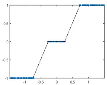
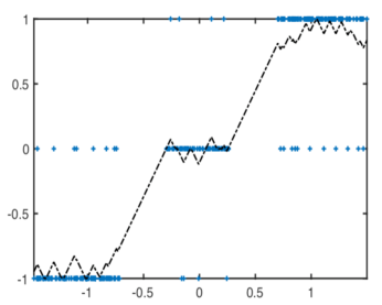
Figure 1. Synthetic labelled data and Lipschitz regularized solution $u$. Left: The solution value matches the labels perfectly on a large portion of the data set. Right: 10% of the data is corrupted by incorrect labels; the regularized solution corrects the errors.

3. Adversarial attacks and defences

Adversarial attacks seek to find a small perturbation of an image vector which leads to a misclassification by the model. Since undefended models are vulnerable to very small norm attacks, the goal of adversarial defence methods is to force successful attack vectors to be larger in size. To allow gradients to be used, the classification attack is usually replaced by an attack on the loss.

The earliest and most successful defence to adversarial perturbations is adversarial training [55, 29, 59, 41, 37]. Adversarial training corresponds to teaching the network to correctly identify adversarially perturbed images by replacing training images $x$ with attacked images $x^{\prime}$. The attacked images used by Madry et al. [41] arise from I-FGSM. However determining the best choice of attack vectors is model dependent, and requires choosing a number of hyperparameters (for example $\varepsilon$ and the number of iterations). Current models trade off model robustness and model accuracy; [60] claims this cannot be avoided.

Focusing on the model loss, ${\ell}(x)$, defined in Section 2.2, adversarial perturbations can be modelled as an optimization problem. For a given adversarial distance, denoted $\varepsilon$, the optimal loss attack on the image vector, $x$, is the solution of

(3.1) $$\max_{\|x^{\prime}-x\|\leq\varepsilon}{\ell}(x^{\prime}).$$

The solution, $x^{\prime}$ is the perturbed image vector within a given distance of $x$, which maximally increases the loss.

The Fast Gradient Sign Method (FGSM) [29] arises when attacks are measured in the $\infty$-norm. It corresponds to a one step attack in the direction $d_{1}$ given by the signed gradient

(3.2) $$(d_{1})_{i}=\frac{\nabla\ell(x)_{i}}{|\nabla\ell(x)_{i}|}.$$

The attack direction (3.2) arises from linearization of the objective in (3.1), which leads to

(3.3) $$\max_{\|d\|_{\infty}\leq 1}d\cdot\nabla{\ell}(x)$$

By inspection, the minimizer is the signed gradient vector, (3.2), and the optimal value is $\|\nabla{\ell}(x)\|_{1}$. When the $2$-norm is used in (3.3), the optimal value is $\|\nabla{\ell}(x)\|_{2}$ and the optimal direction is the normalized gradient

(3.4) $$\dfrac{\nabla\ell(x)}{\|\nabla\ell(x)\|_{2}}.$$

More generally, when a generic norm is used in (3.3), the maximum of the linearized objective is the dual norm [12, A.1.6].

Iterative versions of these attacks lead to respectively Iterative FGSM (I-FGSM) [39], and projected gradient descent in the 2-norm. These attacks require gradients of the loss. However, other attacks use only model gradients (such as the Carlini-Wagner attack [17]), while others use no gradients at all, but only the classification decision of the model (for example the Boundary attack [13]).

3.1. Image vulnerability

Given the model, $f$, and a correctly classified image vector, $x$, how can we predict when it is vulnerable to attack? This question has already been addressed by examining the model Lipschitz constant, which gives a bound on the worst-case adversarial distance [34, 62]. However the Lipschitz constant does not distinguish whether one image $x$ is more vulnerable to attack than another.

We argue that we can compare the vulnerability of different images using the size of the model loss gradient at the image. To do so, we make the simplifying assumption that the attack is a one-step attack. This argument leads to useful results, which we show later are effective even for general attacks. In the case of a one step attack, this argument is reasonable: consider the extreme case of a zero gradient: then the one-step attack does not perturb the image at all. In the other extreme case, of a very large gradient, a small one step attack will change the loss by a large amount.

Given an adversarially perturbed training image $x^{\prime}$, write $x^{\prime}=x+\varepsilon d$, where $d$ is a unit vector, $d$, and $\varepsilon$ is small. Using a Taylor expansion [35] of the loss, we obtain

(3.5) $${\ell}(x^{\prime})={\ell}(x)+\varepsilon d\cdot\nabla{\ell}(x)+\mathcal{O}(\varepsilon^{2}).$$

Substitute $d$ for either the signed gradient (3.2) or the normalized gradient (3.4) in (3.5) to obtain

(3.6) $${\ell}(x+\varepsilon d)={\ell}(x)+\varepsilon\|\nabla{\ell}(x)\|_{*}+\mathcal{O}(\varepsilon^{2})$$

where $*$ is dual to the norm measuring adversarial perturbations. Thus images with larger loss gradients are more vulnerable to gradient attacks. Moreover, the type of attack vector used (either signed gradient or normalized gradient) determines the correct norm in which to measure the vulnerability.

We can go a little further with (3.6), which measures the vulnerability of an image to attack, by asking what is the size perturbation needed to misclassify an image. Set ${\ell}_{0}$ to be the smallest value of the loss for which the image is misclassified. Then, for small values of $\varepsilon$, using (3.6), we can estimate the minimum adversarial distance by

(3.7) $$\varepsilon(x)=\frac{{\ell}_{0}-{\ell}(x)}{\|\nabla{\ell}(x)\|},\quad\text{ when }{\ell}(x)\leq{\ell}_{0}$$

and $\varepsilon(x)=0$ when $x$ is already misclassified. We remark that for the cross entropy loss, $\ell_{0}$ is bounded above by

(3.8) $${\ell}_{0}\leq\log(\text{number of labels}).$$

4. Lipschitz regularization and generalization

4.1. Generic regularizers

Before studying Lipschitz regularization, we step back and consider properties of general regularizers. Let $\mathcal{H}$ be a collection of function $h:X\to Y$ containing the constant functions.

Definition 4.1.

We say $\mathcal{R}:\mathcal{H}\to\mathbb{R}$ is a regularizer if (i) $\mathcal{R}(h)\geq 0$ and (ii) $\mathcal{R}(h)=0$ if and only if $h$ is constant function. For a given loss $L$, define the regularized learning problem

(RLM) $$\min_{f}\{L(f)+\lambda\mathcal{R}(f)\}.$$

The problem (RLM) corresponds to regularized loss minimization (RLM) instead of expected loss minimization (ELM). Define for $\lambda\geq 0$

(4.1) $$f^{\lambda}\in\operatorname*{{arg\,min}}\{L(f)+\lambda\mathcal{R}(f)\}.$$

Remark 4.2.

The loss $L$ in Definition 4.1 would normally be the training loss on a training set, as in Eq. (2.6). In this case, the regularization functional depends on the entire function $f$, and not just the restriction of $f$ to the training data. In practice, it should be evaluated on a validation set, which leads to additional $O(1/\sigma{m})$ error in evaluating it, which is independent of dimension.

Immediately, we can show that we have some good properties of the regularized functional. In the next lemma, we show that for small values of $\lambda$ the minimizers, $f^{\lambda}$ of (RLM) increase the empirical loss at most linearly in $\lambda$. We also show that for large values of $\lambda$ the value of the regularization term goes to zero as $1/\lambda$.

Definition 4.3.

The realizable case is the case where $f^{*}\in\mathcal{H}$, where $f^{*}$ is the true label function. In particular, we can always achieve zero empirical loss. Define $\bar{f}$ to be the average of $f^{*}$ and write $C_{L}=L(\bar{f})$.

Lemma 4.4.

Define $f^{\lambda}$ as in (4.1), and assume the loss is nonnegative. Then for any $\lambda>0$

(4.2) $$\left\{\begin{aligned} L(f^{\lambda})&\leq L(f^{0})+\lambda\mathcal{R}(f^{0})\\ \mathcal{R}(f^{\lambda})&\leq\frac{1}{\lambda}C_{L}\end{aligned}\right.$$

Note in the realizable case, $L(f^{0})=0$.

Proof.

Since $\mathcal{R}(f^{\lambda})\geq 0$ we have

$$L(f^{\lambda})\leq L(f^{\lambda})+\lambda\mathcal{R}(f^{\lambda})\leq L(f^{0})+\lambda\mathcal{R}(f^{0}),$$

which establishes the first inequality in (4.2). For the other inequality, we use the nonnegativity of the loss to find that

$$\lambda\mathcal{R}(f^{\lambda})\leq L(f^{\lambda})+\lambda\mathcal{R}(f^{\lambda})\leq L(\bar{f})=C_{L},$$

which completes the proof. ∎

The previous result gives a bound on the empirical loss of a minimizer of (RLM) for a generic regularizer $\mathcal{R}$, but it does not say anything about the expected loss. However it does say that we can regularize without changing the empirical loss too much. On the other hand, for large values of the regularizer, we expect that $f^{\lambda}$ is going to a constant, which suggests that the generalization gap is small. However, not every regularizer is a good regularizer, since we could have the trivial regularizer

(4.3) $$\mathcal{R}^{0}(h)=\begin{cases}0&h\text{ is constant }\\ 1&\text{ otherwise }\end{cases}$$

which does nothing and then forces the solution to a constant.

4.2. Lipschitz regularization leads to generalization

We now turn to study generalization properties of Lipschitz regularization. Generalization in machine learning refers to bounds on the generalization gap

$$\mathbb{E}_{x\sim\rho}\left[\ell(u_{n}(x),y(x))\right]-\mathbb{E}_{x\sim{\mathcal{D}}_{n}}\left[\ell(u_{n}(x),y(x))\right]$$

where $u_{n}:X\to Y$ denotes the function learned from the training data ${\mathcal{D}}_{n}$ by solving 2.7. We prove something stronger; namely, we prove that the solutions $u_{n}$ converge almost surely as $n\to\infty$ to the solution of a continuum variational problem of the form

(4.4) $$\min_{u:X\to Y}J[u]:=\mathbb{E}_{x\sim\rho}\left[\ell(u(x),y(x))\right]+\lambda\operatorname{Lip}(u).$$

Theorems 4.7 and 4.8 below show uniform convergence, and convergence with a rate in the strongly convex case, both in the limit as the number of training points $n$ tends to $\infty$. While our rates are dimension dependent, they do not depend on the number of layers in the deep neural network.

We now describe our assumptions on the loss and data distribution. We always make the assumption that $\ell(y_{1},y_{2})\geq 0$ for all $y_{1},y_{2}$ with equality if and only if $y_{1}=y_{2}$. We say $\ell(y_{1},y_{2})$ is strictly convex, if it is strictly convex as a function of $y_{1}$ for all values of $y_{2}$. We say $\ell$ is strongly convex with parameter $\theta>0$, if

(4.5) $$\ell(ty_{1}+(1-t)y_{2},y_{0})+\tfrac{\theta}{2}t(1-t)\|y_{1}-y_{2}\|_{Y}^{2}\leq t\ell(y_{1},y_{0})+(1-t)\ell(y_{2},y_{0})$$

holds for all $y_{0},y_{1},y_{2}\in Y$ and $0\leq t\leq 1$.

Remark 4.5.

The standard cross-entropy loss is not strongly convex or Lipschitz continuous. In order to apply our results, we can use the regularized cross entropy loss with parameter $\epsilon>0$,

(4.6) $$\ell^{KL}_{\varepsilon}(y,z)=-\sum_{i=1}^{D}{(z_{i}+\epsilon)}\log\left(\frac{y_{i}+\epsilon}{z_{i}+\epsilon}\right).$$

which is Lipschitz continuous and strongly convex on the probability simplex.

We make the standard manifold assumption [18], and assume the data distribution $\rho$ is a probability density supported on a compact, smooth, $m$-dimensional manifold $\mathcal{M}$ embedded in $X=[0,1]^{d}$, where $m\ll d$. We denote the probability density again by $\rho:\mathcal{M}\to[0,\infty)$. Hence, the data ${\mathcal{D}}_{n}$ is a sequence $x_{1},\dots,x_{n}$ of i.i.d. random variables on $\mathcal{M}$ with probability density $\rho$. For $\lambda>0$ we let $u^{\lambda}$ denote any minimizer of (4.4), that is

$$u^{\lambda}\in\operatorname*{{arg\,min}}_{u:X\to Y}J[u].$$

While $u^{\lambda}$ is not unique, Lemma 4.6 below shows that $u^{\lambda}$ is unique on the data manifold when the loss $\ell$ is strictly convex. Thus, the choice of minimizer $u^{\lambda}$ is unimportant, since Lemma 4.6 guarantees the minimizer is unique on the data manifold, and all minimizers of (4.4) have the same Lipschitz constant.

Lemma 4.6.

Suppose the loss function is strictly convex in $y_{1}$. If $u,v\in W^{1,\infty}(X;Y)$ are two minimizers of (4.4) and $\inf_{\mathcal{M}}\rho>0$ then $u=v$ on $\mathcal{M}$.

We recall that $W^{1,\infty}(X;Y)$ is the space of Lipschitz mappings from $X$ to $Y$.

Proof.

Let $w=(u+v)/2$. Then by convexity of $J$

(4.7) $$J[w]\leq\tfrac{1}{2}J[u]+\tfrac{1}{2}J[v]=\min_{u}J[u].$$

Therefore, $w$ is a minimizer of $J$ and so we have equality above, which yields

$$\int_{\mathcal{M}}\left[\tfrac{1}{2}\ell\left(u,y\right)+\tfrac{1}{2}\ell\left(v,y\right)\right]\rho\,dVol(x)=\int_{\mathcal{M}}\ell\left(\tfrac{1}{2}u+\tfrac{1}{2}v,y\right)\rho\,dVol(x).$$

Since $\ell$ is strictly convex in its first argument, it follows that $u=v$ on $\mathcal{M}$. ∎

We now state our main generalization results.

Theorem 4.7.

Suppose that $\inf_{\mathcal{M}}\rho>0$ and $\ell:Y\times Y\to\mathbb{R}$ is Lipschitz and strictly convex. Then with probability one

(4.8) $$u_{n}\longrightarrow u^{\lambda}\ \ \text{uniformly on }\mathcal{M}\text{ as }n\to\infty,$$

where $u_{n}$ is any sequence of minimizers of (2.7). Furthermore, every uniformly convergent subsequence of $u_{n}$ converges on $X$ to a minimizer of (4.4).

If we also assume strong convexity of the loss, then we get a convergence rate.

Theorem 4.8.

Suppose that $\ell:Y\times Y\to\mathbb{R}$ is Lipschitz and strongly convex. Then for any $t>0$, with probability at least $1-2t^{-\frac{m}{m+2}}n^{-(ct-1)}$ all minimizing sequences $u_{n}$ of (2.7) satisfy

(4.9) $$\frac{\theta}{2}\int_{\mathcal{M}}\|u_{n}-u^{\lambda}\|_{Y}^{2}\rho\,dVol(x)\leq C\lambda^{-1}J[u^{\lambda}]\left(\frac{t\log(n)}{n}\right)^{\frac{1}{m+2}}.$$

In Theorem 4.7 and Theorem 4.8, the sequence $u_{n}$ does not, in general, converge on the whole domain $X$. The important point is that the sequence converges on the data manifold $\mathcal{M}$, and solves the variational problem (4.4) off of the manifold, which provides regularization away from the training data.

Finally, due to the uniform Lipschitzness of the sequence $u_{n}$, which is established in the proof of Theorem 4.8, we can upgrade the $L^{2}$ convergence rate from Theorem 4.8 to an $L^{\infty}$-rate.

Corollary 4.9.

Suppose that $\ell:Y\times Y\to\mathbb{R}$ is Lipschitz and strongly convex. Then for any $t>0$, with probability at least $1-2t^{-\frac{m}{m+2}}n^{-(ct-1)}$ all minimizing sequences $u_{n}$ of (2.7) satisfy

(4.10) $$\|u_{n}-u^{\lambda}\|_{L^{\infty}(\mathcal{M},Y)}^{m+2}\leq Cm^{2}L_{n}^{m}\lambda^{-1}J[u^{\lambda}]\left(\frac{t\log(n)}{n}\right)^{\frac{1}{m+2}},$$

when $\|u_{n}-u^{\lambda}\|_{L^{\infty}(\mathcal{M},Y)}\leq L_{n}r$, and

(4.11) $$\|u_{n}-u^{\lambda}\|^{2}_{L^{\infty}(\mathcal{M},Y)}\leq Cm2^{m}r^{-m}\lambda^{-1}J[u^{\lambda}]\left(\frac{t\log(n)}{n}\right)^{\frac{1}{m+2}},$$

when $\|u_{n}-u^{\lambda}\|_{L^{\infty}(\mathcal{M},Y)}\geq L_{n}r$, where $L_{n}=\operatorname{Lip}(u_{n}-u^{\lambda})$ and $r$ depends only on $\mathcal{M}$.

The proof of Corollary 4.9 follows from Theorem 4.8 and a standard interpolation inequality, which we recall for completeness in Theorem A.1 in §A.

We now turn to the proofs of Theorems 4.7 and 4.8, which require some additional notation and preliminary results. Throughout this section, we write

$$L[u,\mu]:=\mathbb{E}_{x\sim\mu}[\ell(u(x),y(x))]=\int_{X}\ell(u(x),y(x))d\mu(x)$$

where $\mu$ is a probability measure supported on $X$. In particular, write $\rho_{n}:=\frac{1}{n}\sum\delta_{x_{i}}$ for the empirical measure corresponding to ${{\mathcal{D}}}_{n}$, so that $L[u,\rho_{n}]$ is the expected loss on ${{\mathcal{D}}}_{n}$. We also let $C,c>0$ denote positive constants depending only on $\mathcal{M}$, and we assume $C\geq 1$ and $0<c<1$. We follow the analysis tradition of allowing the particular values of $C$ and $c$ to change from line to line, to avoid keeping track of too many constants. Finally, we Let $H_{L}(X;Y)$ denote the collection of $L$-Lipschitz functions $w:X\to Y$.

The proofs of of Theorems 4.7 and 4.8 require a discrepancy result.

Lemma 4.10.

Suppose that $\inf_{\mathcal{M}}\rho>0$, and $dim(\mathcal{M})=m$. Then for any $t>0$

(4.12) $$\sup_{w\in H_{L}(X;Y)}\left|\frac{1}{n}\sum_{i=1}^{n}w(x_{i})-\int_{\mathcal{M}}w\rho\,dVol(x)\right|\leq CL\left(\frac{t\log(n)}{n}\right)^{\frac{1}{m+2}}$$

holds with probability at least $1-2t^{-\frac{m}{m+2}}n^{-(ct-1)}$.

The proof of Lemma 4.10 is given in §B. The estimate (4.12) is called a discrepancy result [56, 33], and is a uniform version of concentration inequalities. The exponent $1/(m+2)$ is not optimal, but affords a very simple proof. It is possible to prove a similar result with the optimal exponent $1/m$ in dimension $m\geq 3$, but the proof is significantly more involved. We refer the reader to [56] for details.

We now give the proof of Theorem 4.7.

Proof of Theorem 4.7.

By Lemma 4.10 the event that

(4.13) $$\lim_{n\to\infty}\sup_{w\in H_{L}(X;Y)}\left|L[w,\rho_{n}]-L[w,\rho]\right|=0$$

for all Lipschitz constants $L>0$ has probability one. For the rest of the proof we restrict ourselves to this event.

Let $u_{n}\in W^{1,\infty}(X;Y)$ be a sequence of minimizers of (2.7), and let $u^{\lambda}\in W^{1,\infty}(X;Y)$ be any minimizer of (4.4). Then since

$$J^{n}[u_{n}]\leq J^{n}[u^{\lambda}]$$

we have

$$L[u_{n},\rho_{n}]+\lambda\operatorname{Lip}(u_{n})\leq+L[u^{\lambda},\rho_{n}]+\lambda\operatorname{Lip}(u^{\lambda}).$$

Write $L_{0}=\operatorname{Lip}(u^{\lambda})$. Then

(4.14) $$\operatorname{Lip}(u_{n})\leq L_{0}+\lambda^{-1}(L[u^{\lambda},\rho_{n}]-L[u_{n},\rho_{n}]).$$

In particular, $\operatorname{Lip}(u_{n})$ is uniformly bounded in $n$. Since the label space $Y$ is compact, the sequence $u_{n}:X\to Y$ is uniformly bounded as well.

By the Arzelà-Ascoli Theorem [50] there exists a subsequence $u_{n_{j}}$ and a function $u\in W^{1,\infty}(X;Y)$ such that $u_{n_{j}}\to u$ uniformly as $n_{j}\to\infty$. Note we also have $\operatorname{Lip}(u)\leq\liminf_{j\to\infty}\operatorname{Lip}(u_{n_{j}})$. Since

$$|L[u_{n},\rho_{n}]-L[u,\rho]| \leq|L[u_{n},\rho_{n}]-L[u,\rho_{n}]|+|L[u,\rho_{n}]-L[u,\rho]|$$

$$\leq C\|u_{n}-u\|_{L^{\infty}(\mathcal{M};Y)}+\sup_{w\in H_{L}(X;Y)}\left|L[w,\rho_{n}]-L[w,\rho]\right|$$

it follows from (4.13) that $L[u_{n_{j}},\rho_{n_{j}}]\to L[u,\rho]$ as $j\to\infty$. It also follows from (4.13) that $J^{n}[u^{\lambda}]\to J[u^{\lambda}]$ as $n\to\infty$. Therefore

$$J[u^{\lambda}] =\lim_{n\to\infty}J^{n}[u^{\lambda}]$$

$$\geq\liminf_{n\to\infty}J^{n}[u_{n}]$$

$$=\liminf_{n\to\infty}L[u_{n},\rho_{n}]+\lambda\operatorname{Lip}(u_{n})$$

$$=\lim_{n\to\infty}L[u_{n},\rho_{n}]+\liminf_{n\to\infty}\lambda\operatorname{Lip}(u_{n})$$

$$\geq L[u,\rho]+\lambda\operatorname{Lip}(u)=J[u].$$

Therefore, $u$ is a minimizer of $J$. By Lemma 4.6, $u=u^{\lambda}$ on $\mathcal{M}$, and so $u_{n_{j}}\to u^{\lambda}$ uniformly on $\mathcal{M}$ as $j\to\infty$.

Now, suppose that (4.8) does not hold. Then there exists a subsequence $u_{n_{j}}$ and $\delta>0$ such that

$$\max_{x\in\mathcal{M}}|u_{n_{j}}(x)-u^{\lambda}(x)|>\delta$$

for all $j\geq 1$. However, we can apply the argument above to extract a further subsequence of $u_{n_{j}}$ that converges uniformly on $\mathcal{M}$ to $u^{\lambda}$, which is a contradiction. This completes the proof. ∎

The proof of Theorem 4.8 requires some additional preliminary setup.

Proposition 4.11.

If $\ell$ is strongly convex with parameter $\theta>0$ then

(4.15) $$J[tu_{1}+(1-t)u_{2}]+\tfrac{\theta}{2}t(1-t)\int_{\mathcal{M}}\|u_{1}-u_{2}\|_{Y}^{2}\rho\,dVol(x)\leq tJ[u_{1}]+(1-t)J[u_{2}]$$

for all $u_{1},u_{2}\in W^{1,\infty}(X;Y)$ and $0\leq t\leq 1$.

Proof.

We compute

$$J[tu_{1}+(1-t)u_{2}] =\int_{\mathcal{M}}\ell(tu_{1}+(1-t)u_{2},y)\rho\,dVol(x)+\lambda\operatorname{Lip}(tu_{1}+(1-t)u_{2})$$

$$\leq tJ[u_{1}]+(1-t)J[u_{2}]-\frac{\theta}{2}t(1-t)\int_{\mathcal{M}}\|u_{1}-u_{2}\|_{Y}^{2}\rho\,dVol(x),$$

which completes the proof. ∎

Lemma 4.12.

If $u^{\lambda}\in W^{1,\infty}(X;Y)$ is a minimizer of (4.4) and $u\in W^{1,\infty}(X;Y)$ then

(4.16) $$\frac{\theta}{2}\int_{\mathcal{M}}\|u-u^{\lambda}\|_{Y}^{2}\rho\,dVol(x)\leq J[u]-J[u^{\lambda}].$$

Proof.

We use Proposition 4.11 with $u_{1}=u^{\lambda}$ and $u_{2}=u$ to obtain

$$J[tu^{\lambda}+(1-t)u]+\frac{\theta}{2}t(1-t)\int_{\mathcal{M}}\|u^{\lambda}-u\|_{Y}^{2}\rho\,dVol(x)\leq tJ[u^{\lambda}]+(1-t)J[u].$$

Since $J[tu^{\lambda}+(1-t)u]\geq J[u^{\lambda}]$

$$J[u^{\lambda}]+\frac{\theta}{2}t(1-t)\int_{\mathcal{M}}\|u^{\lambda}-u\|_{Y}^{2}\rho\,dVol(x)\leq tJ[u^{\lambda}]+(1-t)J[u],$$

and so

$$\frac{\theta}{2}t\int_{\mathcal{M}}\|u^{\lambda}-u\|_{Y}^{2}\rho\,dVol(x)\leq J[u]-J[u^{\lambda}].$$

Setting $t=1$ completes the proof. ∎

We now give the proof of Theorem 4.8.

Proof of Theorem 4.8.

By Lemma 4.10

(4.17) $$\sup_{w\in H_{L_{0}}(X;Y)}\left|L[w,\rho_{n}]-L[w,\rho]\right|\leq CL_{0}\left(\frac{t\log(n)}{n}\right)^{\frac{1}{m+2}}$$

holds with probability at least $1-2t^{-\frac{m}{m+2}}n^{-(ct-1)}$ for any $t>0$. Let us assume for the rest of the proof that (4.17) holds.

By (4.14) in the proof of Theorem 4.7, we have

$$\operatorname{Lip}(u_{n})\leq L_{0}+D_{n},$$

where $D_{n}=\lambda^{-1}(L[u^{\lambda},\rho_{n}]-L[u_{n},\rho_{n}])$. By (4.17) we have

$$D_{n}\leq\lambda^{-1}L[u^{\lambda},\rho]+CL_{0}\left(\frac{t\log(n)}{n}\right)^{\frac{1}{m+2}}.$$

Therefore

(4.18) $$\left|J^{n}[u^{\lambda}]-J[u^{\lambda}]\right|,\left|J^{n}[u_{n}]-J[u_{n}]\right|\leq C(L_{0}+\lambda^{-1}L[u^{\lambda},\rho])\left(\frac{t\log(n)}{n}\right)^{\frac{1}{m+2}},$$

and since $L_{0}+\lambda^{-1}L[u^{\lambda},\rho]=\lambda^{-1}J[u^{\lambda}]$ we have

(4.19) $$J[u_{n}]-J[u^{\lambda}] =J^{n}[u_{n}]-J[u^{\lambda}]+J[u_{n}]-J^{n}[u_{n}]\leq C\lambda^{-1}J[u^{\lambda}]\left(\frac{t\log(n)}{n}\right)^{\frac{1}{m+2}}.$$

By Lemma 4.12 we deduce

$$\frac{\theta}{2}\int_{\mathcal{M}}\|u_{n}-u^{\lambda}\|_{Y}^{2}\rho\,dVol(x)\leq C\lambda^{-1}J[u^{\lambda}]\left(\frac{t\log(n)}{n}\right)^{\frac{1}{m+2}},$$

which completes the proof. ∎

5. Adversarial robustness results

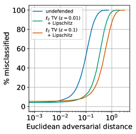
Figure 2. Adversarial robustness results against $\ell_{2}$ PGD attacks using a ResNeXt architecture on the CIFAR-10 test set. The probability of a successful attack is plotted against distance in $\ell_{2}$, for an undefended network and two defended networks.

Table 1. Comparison with other defence methods on CIFAR-10. Misclassification error (percentage) is reported on test images. Each row corresponds to an adversarial attack method.

			Defence method
Attack	details		$\ell_{2}$ TV + Lipschitz			Madry	Qian
			$\varepsilon=0.01$,	$\varepsilon=0.1$,	$\varepsilon=0.1$,
			$\lambda=0.1$	$\lambda=0.1$	$\lambda=1$
test error	undefended model		4.1	4.1	4.1	4.8	5.0
	defended model		4.1	5.4	6.0	12.8	22.8
$\ell_{2}$ PGD	distance	$\|\varepsilon\|_{2}=100/255$	59.8	37.2	36.1	$>90$	-
CW		$\|\varepsilon\|_{2}=1.5$	90.8	91.2	84.4	-	79.6
I-FGSM		$\|\varepsilon\|_{\infty}={8}/{255}$	98.1	91.6	93.7	54.2	-

Table 2. Adversarial statistics with ResNeXt-34 (2x32) on CIFAR-10 test data.

		adversarial distance 2-norm			adversarial distance $\infty$-norm		max test statistics		mean test statistics
defence method	% Err at	median	median	% Err at	median	% Err at	$\|\operatorname{\nabla}\ell\|_{2}$	$\|\operatorname{\nabla}f\|_{2,\infty}$	$\|\operatorname{\nabla}\ell\|_{2}$	$\|\operatorname{\nabla}f\|_{2,\infty}$
	$\varepsilon=0$	distance	time	$\varepsilon=0.1$	distance	$\varepsilon=\frac{8}{255}$
undefended	4.07	0.09	159	53.98	$2.710-3$	100	85.21	13.70	1.90	0.37
$\ell_{1}$ TV (AT, FGSM)	3.87	0.19	301	23.26	$5.610-3$	92.74	35.77	6.27	1.10	0.21
$\ell_{2}$ TV ($\varepsilon=0.01$)	3.58	0.30	471	13.54	$9.010-3$	98.34	32.13	5.22	0.59	0.11
$\ell_{2}$ TV ($\varepsilon=0.01$) + Lipschitz ($\lambda=0.1$)	4.13	0.31	473	12.52	$9.110-3$	98.10	4.10	2.14	0.55	0.10
$\ell_{2}$ TV ($\varepsilon=0.1$) + Lipschitz ($\lambda=0.1$)	5.37	0.48	659	10.31	$13.710-3$	91.6	31.96	8.93	1.19	0.47
$\ell_{2}$ TV ($\varepsilon=0.1$) + Lipschitz ($\lambda=1$)	5.98	0.52	698	10.95	$14.710-2$	93.7	18.53	4.87	1.02	0.46

Table 3. Adversarial statistics with ResNeXt-34 (4x32) on CIFAR-100. Training with $\varepsilon=0.01$ and $\lambda=0.1$

		adversarial distance 2-norm			adversarial distance $\infty$-norm		max test statistics		mean test statistics
defence method	% Err at	median	median	% Err at	median	% Err at	$\|\operatorname{\nabla}\ell\|_{2}$	$\|\operatorname{\nabla}f\|_{2,\infty}$	$\|\operatorname{\nabla}\ell\|_{2}$	$\|\operatorname{\nabla}f\|_{2,\infty}$
	$\varepsilon=0$	distance	time	$\varepsilon=0.1$	distance	$\varepsilon=\frac{1}{255}$
undefended	21.24	$4.710-2$	152	74.18	$1.410-3$	81.52	93.83	1.89	5.19	0.14
$\ell_{1}$ TV (AT, FGSM)	22.06	$8.810-2$	227	53.09	$2.510-3$	63.71	34.60	0.71	2.97	0.08
$\ell_{2}$ TV	21.57	$8.610-2$	253	53.77	$2.610-3$	61.72	44.81	0.73	2.86	0.08
$\ell_{2}$ TV + Lipschitz	21.73	$11.210-2$	307	46.79	$3.210-3$	55.92	27.58	0.46	2.10	0.05

Here we present adversarial robustness results for models trained with the modified loss (2.6) on the CIFAR-10 and CIFAR-100 datasets [38]. We used the ResNeXt architecture [64]. Models were trained with standard data augmentation and training hyper-parameters for the CIFAR datasets, and cutout [22].

Our results are summarized in Tables 2 for CIFAR-10 and 3 for CIFAR-10. We implement four standard attacks using the Foolbox library [48]: PGD in the 2-norm; Iterative FGSM; Boundary attack; and the Carlini-Wagner attack. We found that when measured in the 2-norm, generally PGD was the most effective attack (on our reported models), whereas when measured in the $\infty$-norm, Iterative FGSM was the most effective. See for example Figure 3, where we plot error curves comparing the four attacks, on both our best regularized model and an undefended model. The error curve measures the probability of successful attack given an adversarial distance.

In Tables 2 and 3 we report test error on clean images, and the error at adversarial perturbation $\varepsilon=0.1$ in the 2-norm (just visible to the human eye) and $\varepsilon=8/255$ in the $\infty$-norm. We also report median adversarial distance (which corresponds to the $x$-intercept of 50% on the attack curves). The median adversarial distance is a better overall characterization of adversarial robustness than reporting values at one particular distance.

We also report median time to successful attack (as a ratio over one model call). The median time to attack is a proxy for the cost of a successful attacks. We make an analogy with cryptography [54]: there is no unbreakable code, but there is a code which takes enormous effort to break. Thus, as a secondary goal, we can design models which are costly to attack.

Comparison with other works. On the CIFAR-10 dataset to our knowledge the current state-of-the-art is [41] (using adversarial training) for attacks measured in the $\infty$-norm, and until recently was also the state-of-the-art in the 2-norm. [41] reports results at $\varepsilon=8/255$ in the $\infty$-norm. Comparing with our training hyperparameters set to $\varepsilon=\lambda=0.1$, our model achieved 91.6% error, whereas Madry et al. [41] reports 54.2% error. In the 2-norm, our model achieves 37.2% error at adversarial distance 100/255, whereas Madry et al. [41] reports roughly 90% error at this distance. However, on clean images Madry et al. [41] reported 12.8% test error, whereas we obtain 5.4% versus 4.1% for the undefended model. See Table 1.

We also compare to the more recent work of Qian and Wegman [47] who report strong results for attacks measured in the 2-norm. Qian and Wegman [47] report results only at 2-norm of 1.5, which is a large value. They obtain an error of 79.6%, whereas we achieved around 90% at this distance. However, we note that our regularized model achieves roughly 5% test error, whereas Qian and Wegman [47] report nearly 23% test error. By comparison, at 23% error, we had an adversarial robustness distance of 0.25. Thus at some distance in between .25 and 1.5, the error curves cross, but this crossover point could not be obtained from their data.

Defended models are still accurate. By choosing the hyper-parameters $\varepsilon$ and $\lambda$ (multipliers for respectively the Total Variation and Lipschitz regularizers in (2.6)) judiciously, we are able to train robust models without significantly degrading test error. For some architectures we even observed improved test error. For example, on CIFAR-10, with ResNeXt-34 (2x32), the undefended baseline model achieved 4.07% misclassification error, whereas the regularized model achieved 4.13%. Another regularized model, which had nearly the same robustness, had better accuracy than the baseline, achieving 3.58% See Table 2.

On CIFAR-100, the undefended model achieved 21.2% misclassification, while the most heavily regularized model achieved 21.73% error.

Increasing the amount of regularization leads to worse test accuracy on clean images, but improved adversarial robustness. For example in Figure 2 we plot error curves for three models, with different levels of regularization. The undefended network performs best on clean images, but is not adversarially robust. Of the two regularized networks, the network with strongest regularization ($\varepsilon=0.1$) has better robustness properties than the network regularized with $\varepsilon=0.01$, with respectively adversarial distances of 0.48 and 0.31. However, when measured by test error, the ranking is reversed, with test error 5.37% and 4.13% respectively. Thus a balance may struck depending on the desired outcome, with test error degrading as the level of regularization is increased, consistent with [60].

Defended models are robust to attacks. Defended models have increased median adversarial distance and improved adversarial robustness, as measured by adversarial test accuracy. Models with more regularization leads to stronger adversarial defence, as shown in Tables 2 and 3.

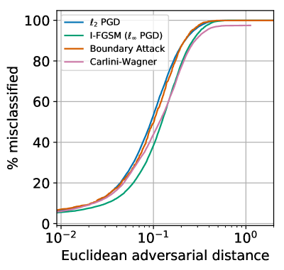
(a) undefended model

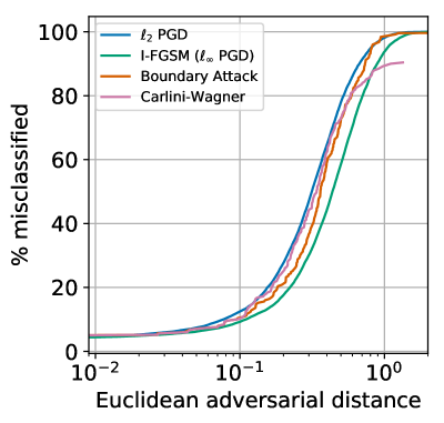
(b) best regularized model

Figure 3. Comparison of attack methods using error curves for ResNeXt-34 (2x32), on the CIFAR-10 test set. The error curve measures the probability of successful attack given an adversarial distance. 3(a) compares attacks on an undefended model; 3(b) compares attacks on our best regularized model.

6. Robustness metrics

Here we demonstrate that the measure of a model’s robustness is given by the Total Variation (average gradient norm) and the Lipschitz constant (maximum gradient) norm of the model, or its loss. This allows us to estimate improved robustness based on the improvement of the Total Variation and the Lipschitz constant of the models. See Table 5.

We estimated the Lipschitz constant of a model (or the loss of a model) using (2.3). This estimate is based on sampling the norm of the gradient on the test data. This leads to an accurate and efficient method for estimating the Lipschitz constant of the model, and the loss of a model. Our empirical estimate (see Tables 2 & 3), was usually close to one, and was at most 14. In contrast, by estimating the Lipschitz constant of a model as a product of weight matrix norms, we obtained values between $10^{12}$ and $10^{23}$. We find that our estimate, (2.3), agrees closely with the Lipschitz constant of the dataset. The Lipschitz constant of a dataset ${\mathcal{D}}$ (in the $2,\infty$ norm) is the reciprocal of the minimum out-of-class $2$-norm distance. Table 4 lists the Lipschitz constant of the training data for common datasets. All datasets have Lipschitz constant close to or below one, which is similar to the estimate of the Lipschitz constant of the model.

Table 4. Lipschitz constants in the ${2,\infty}$ norm, (equivalently $\min\|x_{i}-x_{j}\|$ for images in difference classes), of training sets. For CIFAR-100 we exclude duplicated images.

MNIST	FashionMNIST	CIFAR-10	CIFAR-100
0.417	0.626	0.364	1.245

Table 5. Predicted and actual improvement of a robust regularized model over an undefended model for three measures of robustness. Prediction based on ratio of model Total Variation and model Lipschitz constant. Actual improvement based on ratio of median adversarial distance.

Dataset	Predicted	actual
CIFAR-10	3.4—6.4	3.4
CIFAR-100	2.8—4.1	2.4

We see that penalizing the Lipschitz constant of the loss during model training reduces the Lipschitz constant of the model on the test data. For example, unregularized models had Lipschitz constants of 13.7 and 1.89, on respectively CIFAR-10 and CIFAR-100. In contrast, with Lipschitz regularization these constants reduced to to 2.14 and 0.46. Refer to Tables 2 and 3 for more details. This implies these models are more robust to attack, which we observe reflected in the adversarial perturbation statistics.

A similar reduction is observed in the Total Variation of a model when models are trained with Total Variation regularization. Tables 2 and 3 demonstrate that the median adversarial distance of a model is inversely proportional to the model’s Total Variation. We find that the improvement in median distance of a regularized model over an undefended model corresponds to the relative improvement in the Total Variation of the model. See Table 5.

7. Attack detection

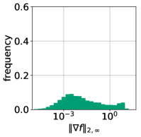
(a) Clean

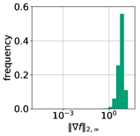
(b) PGD attacked

(c) Boundary attack

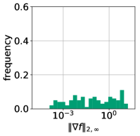
(d) evasive CW attack

Figure 4. Frequency distribution of the norm of the model Jacobian $\|\nabla f(x)\|_{2,\infty}$ on ResNeXt-34 (2x32) on CIFAR-10, using 4(a): Clean, 4(b): PGD attacked 4(c): Boundary attacked, 4(d): evasive-CW attacked test images.

In this section we empirically demonstrate that image vulnerability may also be used to detect adversarial examples. We hypothesize that unless otherwise penalized, gradient based attacks will tend to move images to regions where the gradient of the loss is large. Based on this heuristic, we propose the norm of the loss gradient norm as criterion for detecting adversarial perturbations. Because the loss is not available during inference, we propose using the norm of the model gradient as a rejection criteria: an image has been adversarially perturbed if

(7.1) $$\|\nabla f(x)\|_{2,\infty}\geq c,$$

for some threshold value, $c$. The threshold is determined by setting the significance level (the rate of false positives) to 5%. For example on CIFAR-10 we obtained $c=2.45$ for our model. The results are reported in Table 6 and in Figure 4. Only 6% of clean test images were rejected. However, 100% of Boundary attacks and Carlini-Wagner attacks were detected, as well as 96% of PGD attacked images.

This leads to the question, is it possible to successfully perturb all images in the test set, and avoid detection? We built a targeted attack, designed to avoid detection. Following the recommendation of Athalye et al. [3], we use a Carlini-Wagner (CW) style attack, modified with a penalty to avoid detection. We augmented the attack loss function with a penalty for $\|\nabla{\ell}(x)\|^{2}_{*}$, which penalizes attacks for being detectable. We call this attack an evasive Carlini-Wagner attack. The evasive CW attack was successful at avoiding detection 78% of the time, but in order to do so, it increased the median adversarial distance significantly, from 0.31 to 0.81, see Table 6.

Table 6. Adversarial detection with ResNeXt-34 (2x32) on CIFAR-10. Clean images which the model correctly labels are perturbed until they are misclassified with four attack methods (PGD, Boundary attack, Carlini-Wagner, and an evasive Carlini-Wagner designed to avoid detection). Images are rejected if $\|\nabla f(x)\|_{2,\infty}>2.45$.

	Image source
	clean	PGD	Boundary	CW	evasive CW
attack detected?	6%	96%	100%	100%	22%
median $\ell_{2}$	-	0.31	0.36	0.34	0.81

Appendix A Interpolation inequality

We show here how to estimate the $L^{\infty}$ norm of a function by its $L^{2}$ norm and Lipschitz constant.

Theorem A.1 (Interpolation inequalities).

Let $u:X\to Y$ be Lipschitz continuous with Lipschitz constant $L$. There exists $r>0$ depending only on $\mathcal{M}$ such that when $\|u\|_{L^{\infty}(\mathcal{M},Y)}\leq Lr$ we have

(A.1) $$\|u\|_{L^{\infty}(\mathcal{M},Y)}^{m+2}\leq\frac{(m+2)(m+1)}{\alpha(m)}L^{m}\|u\|_{L^{2}(\mathcal{M},Y)}^{2},$$

and when $\|u\|_{L^{\infty}(\mathcal{M},Y)}\geq Lr$ we have

(A.2) $$\|u\|^{2}_{L^{\infty}(\mathcal{M},Y)}\leq\frac{2^{m+1}(m+1)}{\alpha(m)r^{m}}\|u\|_{L^{2}(\mathcal{M},Y)}^{2},$$

where $\alpha(m)$ is the volume of the unit ball in $\mathbb{R}^{m}$.

Proof.

We may assume, without loss of generality, that $Y=\mathbb{R}$. Let $x_{0}\in\mathcal{M}$ such that $|u|$ attains its max over $\mathcal{M}$ at $x_{0}$, and assume that $u(x_{0})>0$. Then for any $r>0$ sufficiently small, depending only on $\mathcal{M}$, the Riemannian exponential map $\exp_{x_{0}}:B(0,r)\subset T_{x_{0}}\mathcal{M}\to\mathcal{M}$ is a diffeomorphism between the ball $B(0,r)$ and the geodesic ball $B_{\mathcal{M}}(x_{0},r)$, the Jacobian of $\exp_{x_{0}}$, denoted $J_{x_{0}}(v)$ satisfies $J_{x_{0}}(v)\geq\frac{1}{2}$ for all $|v|\leq r$, and the geodesic distance $d(x,x_{0}$ satisfies $d(x,x_{0})\geq|x-x_{0}|$. Writing $K=\|u\|_{L^{\infty}(\mathcal{M},Y)}=u(x_{0})$, we we have

$$\|u\|^{2}_{L^{2}(\mathcal{M},Y)} \geq\int_{B_{\mathcal{M}}(x_{0},r)}u(x)^{2}\,dVol(x)$$

$$\geq\int_{B_{\mathcal{M}}(x_{0},r)}(K-L|x-x_{0}|)_{+}^{2}\,dVol(x)$$

$$\geq\int_{B_{\mathcal{M}}(x_{0},r)}(K-Ld(x,x_{0}))_{+}^{2}\,dVol(x)$$

$$=\int_{B(0,r)\subset T_{x_{0}}\mathcal{M}}(K-L|v|)_{+}^{2}J_{x_{0}}(v)\,dv,$$

$$\geq\frac{1}{2}\int_{B(0,r)}(K-L|v|)_{+}^{2}\,dv.$$

If $r\geq K/L$ then we can compute

$$\int_{B(0,r)}(K-L|v|)_{+}^{2}\,dv=\frac{2\alpha(m)}{(m+2)(m+1)}\frac{K^{m+2}}{L^{m}}.$$

This yields the estimate

$$\|u\|_{L^{\infty}(\mathcal{M},Y)}^{m+2}\leq\frac{(m+2)(m+1)}{\alpha(m)}L^{m}\|u\|_{L^{2}(\mathcal{M},Y)}^{2}.$$

If $r\leq K/L$ then we compute

$$\int_{B(0,r)}(K-L|v|)_{+}^{2}\,dv\geq\frac{\alpha(m)r^{m}}{2^{m}(m+1)}K^{2},$$

which yields

$$\|u\|^{2}_{L^{\infty}(\mathcal{M},Y)}\leq\frac{2^{m+1}(m+1)}{\alpha(m)r^{m}}\|u\|_{L^{2}(\mathcal{M},Y)}^{2},$$

which completes the proof. ∎

Appendix B Proof of Lemma 4.10

We give here the proof of Lemma 4.10. A key tool in the proof is Bernstein’s inequality [10], which we recall now for the reader’s convenience. For $X_{1},\dots,X_{n}$ i.i.d. with variance $\sigma^{2}=\mathbb{E}[(X_{i}-\mathbb{E}[X_{i}])^{2}]$, if $|X_{i}|\leq M$ almost surely for all $i$ then Bernstein’s inequality states that for any $\varepsilon>0$

(B.1) $$\mathbb{P}\left(\left|\frac{1}{n}\sum_{i=1}^{n}X_{i}-\mathbb{E}[X_{i}]\right|>\varepsilon\right)\leq 2\exp\left(-\frac{n\varepsilon^{2}}{2\sigma^{2}+4M\varepsilon/3}\right).$$

Proof of Lemma 4.10.

We note that it is sufficient to prove the result for $w\in H_{L}(X;Y)$ with $\int_{\mathcal{M}}w\rho\,dVol(x)=0$. In this case, we have $w(x)=0$ for some $x\in\mathcal{M}$, and so $\|w\|_{L^{\infty}(X;Y)}\leq CL$.

We first give the proof for $\mathcal{M}=X=[0,1]^{m}$. We partition $X$ into hypercubes $B_{1},\dots,B_{N}$ of side length $h>0$, where $N=h^{-m}$. Let $Z_{j}$ denote the number of $x_{1},\dots,x_{n}$ falling in $B_{j}$. Then $Z_{j}$ is a Binomial random variable with parameters $n$ and $p_{j}=\int_{B_{j}}\rho\,dx\geq ch^{m}$. By the Bernstein inequality we have for each $j$ that

(B.2) $$\mathbb{P}\left(\left|\frac{1}{n}Z_{j}-\int_{B_{j}}\rho\,dx\right|>\varepsilon\right)\leq 2\exp\left(-cnh^{-m}\varepsilon^{2}\right)$$

provided $0<\varepsilon\leq h^{m}$. Therefore, we deduce

$$\frac{1}{n}\sum_{i=1}^{n}w(x_{i}) \leq\frac{1}{n}\sum_{j=1}^{N}Z_{j}\max_{B_{j}}w$$

$$\stackrel{{\scriptstyle\eqref{eq:bernapp}}}{{\leq}}\sum_{j=1}^{N}\left(\int_{B_{j}}\rho\,dx+\varepsilon\right)\max_{B_{j}}w$$

$$\leq\sum_{j=1}^{N}\max_{B_{j}}w\int_{B_{j}}\rho\,dx+CLh^{-m}\varepsilon$$

$$\leq\sum_{j=1}^{N}(\min_{B_{j}}w+CLh)\int_{B_{j}}\rho\,dx+CLh^{-m}\varepsilon$$

$$\leq\sum_{j=1}^{N}\int_{B_{j}}w\rho\,dx+CLh^{-m}(h^{m+1}+\varepsilon)$$

$$=\int_{X}w\rho\,dx+CL(h+h^{-m}\varepsilon)$$

holds with probability at least $1-2h^{-m}\exp\left(-cnh^{-m}\varepsilon^{2}\right)$ for any $0<\varepsilon\leq h^{m}$. Choosing $\varepsilon=h^{m+1}$ we have that

(B.3) $$\left|\frac{1}{n}\sum_{i=1}^{n}w(x_{i})-\int_{X}w\rho\,dx\right|\leq CLh$$

holds for all $u\in H_{L}(X;Y)$ with probability at least $1-2h^{-m}\exp\left(-cnh^{m+2}\right)$, provided $h\leq 1$. By selecting $nh^{m+2}=t\log(n)$

$$\sup_{w\in H_{L}(X;Y)}\left|\frac{1}{n}\sum_{i=1}^{n}w(x_{i})-\int_{\mathcal{M}}w\rho\,dVol(x)\right|\leq CL\left(\frac{t\log(n)}{n}\right)^{\frac{1}{m+2}}$$

holds with probability at least $1-2t^{-\frac{m}{m+2}}n^{-(ct-1)}$ for $t\leq n/\log(n)$. Since we have $\|w\|_{L^{\infty}(X;Y)}\leq CL$, the estimate

$$\sup_{w\in H_{L}(X;Y)}\left|\frac{1}{n}\sum_{i=1}^{n}w(x_{i})-\int_{\mathcal{M}}w\rho\,dVol(x)\right|\leq CL,$$

trivially holds, and hence we can allow $t>n/\log(n)$ as well.

We sketch here how to prove the result on the manifold $\mathcal{M}$. We cover $\mathcal{M}$ with $k$ geodesic balls of radius $\varepsilon>0$, denoted $B_{\mathcal{M}}(x_{1},\varepsilon),\dots,B_{\mathcal{M}}(x_{k},\varepsilon)$, and let $\varphi_{1},\dots,\varphi_{k}$ be a partition of unity subordinate to this open covering of $\mathcal{M}$. For $\varepsilon>0$ sufficiently small, the Riemannian exponential map $\exp_{x}:B(0,\varepsilon)\subset T_{x}\mathcal{M}\to\mathcal{M}$ is a diffeomorphism between the ball $B(0,\varepsilon)\subset T_{x}\mathcal{M}$ and the geodesic ball $B_{\mathcal{M}}(x,\varepsilon)\subset\mathcal{M}$, where $T_{x}\mathcal{M}\cong\mathbb{R}^{m}$. Furthermore, the Jacobian of $\exp_{x}$ at $v\in B(0,r)\subset T_{x}\mathcal{M}$, denoted by $J_{x}(v)$, satisfies (by the Rauch Comparison Theorem)

(B.4) $$(1+C|v|^{2})^{-1}\leq J_{x}(v)\leq 1+C|v|^{2}.$$

Therefore, we can run the argument above on the ball $B(0,r)\subset\mathbb{R}^{m}$ in the tangent space, lift the result to the geodesic ball $B_{\mathcal{M}}(x_{i},\varepsilon)$ via the Riemannian exponential map $\exp_{x}$, and apply the bound

$$\left|\frac{1}{n}\sum_{i=1}^{n}w(x_{i})-\int_{\mathcal{M}}w\rho\,dVol(x)\right|\leq\sum_{j=1}^{k}\left|\frac{1}{n}\sum_{i=1}^{n}\varphi_{j}(x_{i})w(x_{i})-\int_{\mathcal{M}}\varphi_{j}w\rho\,dVol(x)\right|$$

to complete the proof. ∎

References

- [1] C. Anil, J. Lucas, and R. Grosse. Sorting out lipschitz function approximation. CoRR, abs/1811.05381, 2018.
- [2] G. Aronsson, M. Crandall, and P. Juutinen. A tour of the theory of absolutely minimizing functions. Bulletin of the American mathematical society, 41(4):439–505, 2004.
- [3] A. Athalye, N. Carlini, and D. Wagner. Obfuscated gradients give a false sense of security: Circumventing defenses to adversarial examples. In J. Dy and A. Krause, editors, Proceedings of the 35th International Conference on Machine Learning, volume 80 of Proceedings of Machine Learning Research, pages 274–283, Stockholmsmässan, Stockholm Sweden, 10–15 Jul 2018. PMLR.
- [4] G. Aubert and P. Kornprobst. Mathematical problems in image processing: Partial Differential Equations and the Calculus of Variations, volume 147. Springer Science & Business Media, 2006.
- [5] P. L. Bartlett. For valid generalization the size of the weights is more important than the size of the network. In Advances in Neural Information Processing Systems 9, NIPS, Denver, CO, USA, December 2-5, 1996, pages 134–140, 1996.
- [6] P. L. Bartlett, D. J. Foster, and M. J. Telgarsky. Spectrally-normalized margin bounds for neural networks. In Advances in Neural Information Processing Systems, pages 6240–6249, 2017.
- [7] M. Bertalmio, G. Sapiro, V. Caselles, and C. Ballester. Image Inpainting. In Proceedings of the 27th annual conference on Computer graphics and interactive techniques, pages 417–424. ACM Press/Addison-Wesley Publishing Co., 2000.
- [8] B. Biggio, I. Corona, D. Maiorca, B. Nelson, N. Šrndi, P. Laskov, G. Giacinto, and F. Roli. Evasion attacks against machine learning at test time. In H. Blockeel, K. Kersting, S. Nijssen, and F. Železný, editors, Machine Learning and Knowledge Discovery in Databases, pages 387–402, Berlin, Heidelberg, 2013. Springer Berlin Heidelberg.
- [9] C. M. Bishop. Training with noise is equivalent to tikhonov regularization. Neural computation, 7(1):108–116, 1995.
- [10] S. Boucheron, G. Lugosi, and P. Massart. Concentration inequalities: A nonasymptotic theory of independence. Oxford university press, 2013.
- [11] O. Bousquet and A. Elisseeff. Stability and generalization. Journal of Machine Learning Research, 2:499–526, 2002.
- [12] S. Boyd and L. Vandenberghe. Convex Optimization. Cambridge University press, 2004.
- [13] W. Brendel, J. Rauber, and M. Bethge. Decision-based adversarial attacks: Reliable attacks against black-box machine learning models. In International Conference on Learning Representations, 2018.
- [14] J. Calder. Consistency of lipschitz learning with infinite unlabeled data and finite labeled data. arXiv preprint arXiv:1710.10364, 2017.
- [15] J. Calder. The game theoretic p-Laplacian and semi-supervised learning with few labels. Nonlinearity, 32(1), 2018.
- [16] N. Carlini and D. A. Wagner. Adversarial examples are not easily detected: Bypassing ten detection methods. In Proceedings of the 10th ACM Workshop on Artificial Intelligence and Security, AISec@CCS 2017, Dallas, TX, USA, November 3, 2017, pages 3–14, 2017.
- [17] N. Carlini and D. A. Wagner. Towards evaluating the robustness of neural networks. In 2017 IEEE Symposium on Security and Privacy, SP 2017, San Jose, CA, USA, May 22-26, 2017, pages 39–57, 2017.
- [18] O. Chapelle, B. Scholkopf, and A. Zien. Semi-supervised learning. MIT, 2006.
- [19] M. Cissé , P. Bojanowski, E. Grave, Y. Dauphin, and N. Usunier. Parseval networks: Improving robustness to adversarial examples. In Proceedings of the 34th International Conference on Machine Learning, ICML 2017, Sydney, NSW, Australia, 6-11 August 2017, pages 854–863, 2017.
- [20] Z. Cranko, S. Kornblith, Z. Shi, and R. Nock. Lipschitz Networks and Distributional Robustness. CoRR, Sept. 2018.
- [21] B. Dacorogna. Direct methods in the calculus of variations, volume 78. Springer Science & Business Media, 2007.
- [22] T. Devries and G. W. Taylor. Improved regularization of convolutional neural networks with cutout. CoRR, abs/1708.04552, 2017.
- [23] H. Drucker and Y. Le Cun. Improving generalization performance using double backpropagation. IEEE Transactions on Neural Networks, 3(6):991–997, 1992.
- [24] A. El Alaoui, X. Cheng, A. Ramdas, M. J. Wainwright, and M. I. Jordan. Asymptotic behavior ofell_p-based laplacian regularization in semi-supervised learning. In Conference on Learning Theory, pages 879–906, 2016.
- [25] C. Elion and L. A. Vese. An image decomposition model using the total variation and the infinity laplacian. In Computational Imaging V, volume 6498, page 64980W. International Society for Optics and Photonics, 2007.
- [26] L. C. Evans. Partial differential equations, volume 19 of Graduate Studies in Mathematics. American Mathematical Society, 1998.
- [27] L. C. Evans. Measure theory and fine properties of functions. Routledge, 2018.
- [28] I. Goodfellow, P. McDaniel, and N. Papernot. Making machine learning robust against adversarial inputs. Communications of the ACM, 61(7):56–66, June 2018.
- [29] I. J. Goodfellow, J. Shlens, and C. Szegedy. Explaining and harnessing adversarial examples. CoRR, abs/1412.6572, 2014.
- [30] H. Gouk, E. Frank, B. Pfahringer, and M. Cree. Regularisation of neural networks by enforcing lipschitz continuity. CoRR, abs/1804.04368, 2018.
- [31] L. Guillot and C. Le Guyader. Extrapolation of vector fields using the infinity laplacian and with applications to image segmentation. In X.-C. Tai, K. Mørken, M. Lysaker, and K.-A. Lie, editors, Scale Space and Variational Methods in Computer Vision, pages 87–99, Berlin, Heidelberg, 2009. Springer Berlin Heidelberg.
- [32] I. Gulrajani, F. Ahmed, M. Arjovsky, V. Dumoulin, and A. C. Courville. Improved Training of Wasserstein GANs. In Advances in Neural Information Processing Systems 30: Annual Conference on Neural Information Processing Systems 2017, 4-9 December 2017, Long Beach, CA, USA, pages 5769–5779, 2017.
- [33] L. Györfi, M. Kohler, A. Krzyzak, and H. Walk. A distribution-free theory of nonparametric regression. Springer Science & Business Media, 2006.
- [34] M. Hein and M. Andriushchenko. Formal Guarantees on the Robustness of a Classifier against Adversarial Manipulation. In Advances in Neural Information Processing Systems 30: Annual Conference on Neural Information Processing Systems 2017, 4-9 December 2017, Long Beach, CA, USA , pages 2263–2273, 2017.
- [35] A. Iserles. A first course in the numerical analysis of differential equations. Number 44. Cambridge university press, 2009.
- [36] W. B. Johnson and J. Lindenstrauss. Extensions of Lipschitz mappings into a Hilbert space. Contemporary Mathematics, 26(189-206):1, 1984.
- [37] H. Kannan, A. Kurakin, and I. J. Goodfellow. Adversarial logit pairing. CoRR, abs/1803.06373, 2018.
- [38] A. Krizhevsky and G. Hinton. Learning multiple layers of features from tiny images. Technical report, University of Toronto, 2009.
- [39] A. Kurakin, I. J. Goodfellow, and S. Bengio. Adversarial examples in the physical world. CoRR, abs/1607.02533, 2016.
- [40] R. Kyng, A. Rao, S. Sachdeva, and D. A. Spielman. Algorithms for lipschitz learning on graphs. In Conference on Learning Theory, pages 1190–1223, 2015.
- [41] A. Madry, A. Makelov, L. Schmidt, D. Tsipras, and A. Vladu. Towards deep learning models resistant to adversarial attacks. CoRR, abs/1706.06083, 2017.
- [42] E. J. McShane. Extension of range of functions. Bulletin of the American Mathematical Society, 40(12):837–842, 1934.
- [43] T. Miyato, T. Kataoka, M. Koyama, and Y. Yoshida. Spectral normalization for generative adversarial networks. In International Conference on Learning Representations, 2018.
- [44] T. Miyato, T. Kataoka, M. Koyama, and Y. Yoshida. Spectral normalization for generative adversarial networks. CoRR, abs/1802.05957, 2018.
- [45] T. Miyato, S.-i. Maeda, M. Koyama, and S. Ishii. Virtual adversarial training: a regularization method for supervised and semi-supervised learning. IEEE transactions on pattern analysis and machine intelligence, 41(8):1979–1993, 2018.
- [46] T. Pock, D. Cremers, H. Bischof, and A. Chambolle. Global solutions of variational models with convex regularization. SIAM Journal on Imaging Sciences, 3(4):1122–1145, 2010.
- [47] H. Qian and M. N. Wegman. L2-nonexpansive neural networks. CoRR, abs/1802.07896, 2018.
- [48] J. Rauber, W. Brendel, and M. Bethge. Foolbox v0.8.0: A Python toolbox to benchmark the robustness of machine learning models. CoRR, abs/1707.04131, 2017.
- [49] L. I. Rudin, S. Osher, and E. Fatemi. Nonlinear Total Variation based noise removal algorithms. Physica D: nonlinear phenomena, 60(1-4):259–268, 1992.
- [50] W. Rudin. Principles of mathematical analysis. McGraw-hill New York, 1976.
- [51] S. Shalev-Shwartz and S. Ben-David. Understanding Machine Learning: From Theory to Algorithms. Cambridge University Press, 2014.
- [52] D. Slepcev and M. Thorpe. Analysis of p-laplacian regularization in semi-supervised learning. arXiv preprint arXiv:1707.06213, 2017.
- [53] J. Sokolic, R. Giryes, G. Sapiro, and M. R. D. Rodrigues. Robust large margin deep neural networks. IEEE Trans. Signal Processing, 65(16):4265–4280, 2017.
- [54] W. Stallings. Cryptography and Network Security, 4/E. Pearson Education India, 2006.
- [55] C. Szegedy, W. Zaremba, I. Sutskever, J. Bruna, D. Erhan, I. J. Goodfellow, and R. Fergus. Intriguing properties of neural networks. CoRR, abs/1312.6199, 2013.
- [56] M. Talagrand. The generic chaining: upper and lower bounds of stochastic processes. Springer Science & Business Media, 2006.
- [57] A. Tikhonov and V. Y. Arsenin. Solutions of Ill-Posed Problems. Winston and Sons, New York, 1977.
- [58] M. Torkamani and D. Lowd. Convex adversarial collective classification. In International Conference on Machine Learning, pages 642–650, 2013.
- [59] F. Tramèr, A. Kurakin, N. Papernot, I. Goodfellow, D. Boneh, and P. McDaniel. Ensemble adversarial training: Attacks and defenses. In International Conference on Learning Representations, 2018.
- [60] D. Tsipras, S. Santurkar, L. Engstrom, A. Turner, and A. Madry. Robustness may be at odds with accuracy. CoRR, abs/1805.12152, 2018.
- [61] Y. Tsuzuku, I. Sato, and M. Sugiyama. Lipschitz-margin training: Scalable certification of perturbation invariance for deep neural networks. CoRR, abs/1802.04034, 2018.
- [62] T.-W. Weng, H. Zhang, P.-Y. Chen, J. Yi, D. Su, Y. Gao, C.-J. Hsieh, and L. Daniel. Evaluating the robustness of neural networks: An extreme value theory approach. In International Conference on Learning Representations, 2018.
- [63] K. Y. Xiao, V. Tjeng, N. M. Shafiullah, and A. Madry. Training for faster adversarial robustness verification via inducing relu stability. CoRR, abs/1809.03008, 2018.
- [64] S. Xie, R. B. Girshick, P. Dollá r, Z. Tu, and K. He. Aggregated residual transformations for deep neural networks. In 2017 IEEE Conference on Computer Vision and Pattern Recognition, CVPR 2017, Honolulu, HI, USA, July 21-26, 2017, pages 5987–5995, 2017.
- [65] H. Xu and S. Mannor. Robustness and generalization. Machine Learning, 86(3):391–423, 2012.