Geometries of edge and mixed dislocations in bcc Fe from first principles calculations

Abstract

We use density functional theory (DFT) to compute the core structures of $a_{0}[100](010)$ edge, $a_{0}[100](011)$ edge, $a_{0}/2[\bar{1}\bar{1}1](1\bar{1}0)$ edge, and $a_{0}/2[111](1\bar{1}0)$ $71^{\circ}$ mixed dislocations in body-centered cubic (bcc) Fe. The calculations are performed using flexible boundary conditions (FBC), which effectively allow the dislocations to relax as isolated defects by coupling the DFT core to an infinite harmonic lattice through the lattice Green function (LGF). We use the LGFs of the dislocated geometries in contrast to most previous FBC-based dislocation calculations that use the LGF of the bulk crystal. The dislocation LGFs account for changes in the topology of the crystal in the core as well as local strain throughout the crystal lattice. A simple bulk-like approximation for the force constants in a dislocated geometry leads to dislocation LGFs that optimize the core structures of the $a_{0}[100](010)$ edge, $a_{0}[100](011)$ edge, and $a_{0}/2[111](1\bar{1}0)$ $71^{\circ}$ mixed dislocations. This approximation fails for the $a_{0}/2[\bar{1}\bar{1}1](1\bar{1}0)$ dislocation however, so in this case we derive the LGF from more accurate force constants computed using a Gaussian approximation potential. The standard deviations of the dislocation Nye tensor distributions quantify the widths of the dislocation cores. The relaxed cores are compact, and the local magnetic moments on the Fe atoms closely follow the volumetric strain distributions in the cores. We also compute the core structures of these dislocations using eight different classical interatomic potentials, and quantify symmetry differences between the cores using the Fourier coefficients of their Nye tensor distributions. Most of the core structures computed using the classical potentials agree well with the DFT results. The DFT core geometries provide benchmarking for classical potential studies of work-hardening, as well as substitutional and interstitial sites for computing solute-dislocation interactions that serve as inputs for mesoscale models of solute strengthening and solute diffusion near dislocations.

I Introduction

Steel alloys are used in a wide variety of structural applications due to their low cost and the relative ease of tuning their mechanical properties via alloying and processing compared to many other structural materials Leslie (1991); Berns and Theisen (2008). The ferrite phase found in many steels is body-centered cubic (bcc) Fe containing C and other solute atoms Leslie (1991); Berns and Theisen (2008); Devaraj et al. (2018). As in other bcc metals, dislocation slip is one of the most important plastic deformation mechanisms in bcc Fe Christian (1983); Taylor (1992). Therefore, accurate modeling of dislocation structures in Fe and their response to stress is key to understanding deformation behavior, improving microstructure-based models of plasticity and fracture, and ultimately developing new steels with improved mechanical properties. The $a_{0}/2\langle 111\rangle$-type screw dislocations in bcc metals have been widely studied since these dislocations largely control the low-temperature plastic deformation of bcc metals and alloys Christian (1983); Duesbery (1989); Taylor (1992). The details of the screw dislocation core structure are known to affect the Peierls stress and therefore the mobility of these dislocations Cai et al. (2004); Chaussidon et al. (2006); Gordon et al. (2010), and density functional theory (DFT) calculations first revealed that the core is compact and symmetric compared to the degenerate core structure predicted by many classical interatomic potentials Ismail-Beigi and Arias (2000); Woodward and Rao (2001, 2002); Frederiksen and Jacobsen (2003). The questionable reliability of classical potentials and the lack of experimental measurements of dislocation core structures in Fe highlights the need for electronic structure methods to compute detailed atomic-level structural features in dislocation cores.

While $a_{0}/2\langle 111\rangle$ screw dislocations predominantly govern the plastic response of bcc metals at low temperatures, dislocations of edge or mixed character may also play important roles in controlling plastic deformation in bcc metals. For example, edge dislocations in bcc metals can form from reactions of dislocations with $a_{0}/2\langle 111\rangle$-type Burgers vectors. As screw dislocations move through the material, they can react with other dislocations intersecting their glide plane and form stable binary junctions with Burgers vector $a_{0}\langle 100\rangle$ via a reaction of type Püschl (1985); Schoeck and Romaner (2010)

$$a_{0}/2[111]+a_{0}/2[1\bar{1}\bar{1}]\rightarrow a_{0}[100].$$ (1)

These binary junctions may themselves be mobile, or further react with other dislocations to form ternary junctions which contribute to work hardening. These junction reactions are of interest and have been studied by dislocation dynamics simulations Bulatov et al. (2006); Madec and Kubin (2008). Here, we consider two possible edge dislocations with $a_{0}\langle 100\rangle$-type Burgers vectors—$a_{0}\langle 100\rangle\{010\}$ and $a_{0}\langle 100\rangle\{011\}$—along with a $a_{0}/2\langle 111\rangle\{011\}$ edge dislocation, as this is the most commonly observed type of edge dislocation in bcc Fe Clouet et al. (2008). Edge dislocations are also of interest for understanding the influence of dislocation loops Bonny et al. (2016); Fikar et al. (2017) and cell structures S.M. Hafez Haghighat et al. (2014a) on deformation processes in Fe. Experimentally observed edge dislocations in nanocrystalline samples of bcc W Wei et al. (2006) and Ta Wei et al. (2011) are believed to be the primary reason for the reported lower strain rate sensitivity of nanocrystalline bcc metals and alloys compared to their coarse-grained counterparts, and may play an important role in controlling the plastic response of nanocrystalline bcc Fe. Finally, dislocations in bcc Fe can play a part in other interesting phenomena as well. For example, pipe diffusion (i.e. accelerated diffusion along the dislocation line) of C interstitials has been predicted to occur in the $a_{0}/2[111](1\bar{1}0)$ $71^{\circ}$ mixed dislocation in bcc Fe Ishii et al. (2013). However, straightforward pipe diffusion was not predicted for other types of dislocations—the migration of C interstitials was found to be accelerated not along the dislocation line direction but in a conjugate diffusion direction formed by a pathway of octahedral interstitial sites adjacent to the dislocation core. In order to better understand the complex mechanisms that are likely to be at play here, accurate and detailed descriptions of the dislocation cores are necessary.

In this study, we use DFT combined with flexible boundary conditions (FBC) Sinclair et al. (1978); Rao et al. (1998); Woodward (2005) to optimize the core structures of the $a_{0}[100](010)$ edge, $a_{0}[100](011)$ edge, $a_{0}/2[\bar{1}\bar{1}1](1\bar{1}0)$ edge, and $a_{0}/2[111](1\bar{1}0)$ $71^{\circ}$ mixed dislocations in bcc Fe. Previous simulations of edge and mixed dislocations in bcc Fe have relied on classical interatomic potentials due to the large supercells needed to contain the long-ranged strain fields generated by dislocations Ishii et al. (2013); Hu et al. (2000); Clouet et al. (2008); Monnet and Terentyev (2009); Queyreau et al. (2011); Terentyev et al. (2011); Wang et al. (2013); Swinburne et al. (2013); Bhatia et al. (2014); S.M. Hafez Haghighat et al. (2014a, b); Bonny et al. (2016); Anento et al. (2018). Yan et al. Yan et al. (2004) and Chen et al. Chen et al. (2006) used first-principles calculations to study the electronic effects of C solutes and kinks on edge dislocations in bcc Fe, respectively. However, both of these studies used a Finnis-Sinclair classical potential to generate the initial dislocation geometries for the first-principles calculations. The accuracy of results from classical simulations strongly depends on the fidelity of the interatomic potential, and there are no experimental measurements or first-principles calculations of edge and mixed dislocation core structures in bcc Fe to benchmark the core structures from classical potentials. We therefore present the first fully ab initio calculations of the core structures of edge and mixed dislocations in bcc Fe. Our DFT-based FBC calculations allow a single dislocation to effectively relax as an isolated defect in a supercell size tractable for DFT calculations by coupling the DFT core to an infinite harmonic lattice through the lattice Green function (LGF) Sinclair et al. (1978); Rao et al. (1998); Woodward (2005); Trinkle (2008). In contrast to most previous DFT-based FBC calculations of dislocation cores that used the LGF of the bulk crystal to approximate the LGF of dislocated geometries, here we use LGFs specifically computed for each dislocation Tan and Trinkle (2016). The dislocation LGFs account for changes in both the topology of the crystal lattice in the highly-distorted core region and local strain throughout the lattice. The FBC method removes any reliance on dislocation multipole arrangements often used in DFT simulations to cancel the long-ranged strain fields generated by dislocations, but that may generate artifacts in the dislocation core structures due to dislocation-dislocation interactions. Our DFT core structures serve to benchmark the predictions of existing potentials, provide fitting data for generating new classical potentials, serve as a basis of comparison for future experimental investigations of dislocation cores in bcc Fe, and also serve as the starting point for first-principles calculations of solution strengthening Yasi et al. (2010) and solute transport near edge and mixed dislocations in bcc Fe Schiavone and Trinkle (2016).

The rest of this paper is organized as follows. Section II presents our computational geometries, discusses the FBC method, and gives the details of our DFT calculations. Here we discuss how we visualize the dislocation cores using a combination of differential displacement maps Vítek et al. (1970), Nye tensor distributions Hartley and Mishin (2005a, b), volumetric strain, and changes in the magnetic moments on the Fe atoms. This section also presents how we quantify the widths of the dislocation cores using the second moments of the Nye tensor distributions, and how we distinguish symmetry differences between the core structures from DFT and classical potentials using the Fourier coefficients of the Nye tensor distributions. Section III presents our DFT-optimized dislocation cores, and compares the results to core structures optimized using eight different interatomic potentials. Section IV summarizes our results and provides further discussion.

II Computational methods

II.1 First principles calculations with flexible boundary conditions

Figure 1 shows the initial dislocation geometries that we optimize using first-principles calculations with FBC. We construct cylindrical slab geometries and introduce the dislocations by displacing all the atoms in the slabs according to the displacement fields predicted by anisotropic elasticity theory Bacon et al. (1980). The magenta “+” symbols in the figure show the center of the elastic displacement field for each dislocation. The displacement fields of edge and mixed dislocations are incompatible with periodic boundary conditions perpendicular to the dislocation threading direction (pointing out of the page), so we surround each slab by a vacuum region. We divide each slab into region 1 (blue), region 2 (red), and region 3 (yellow) for applying FBC which we discuss in the next paragraph. The supercell dimensions perpendicular to the threading directions are equal for all the dislocations, with dimensions of 50.46 Å $\times$ 50.46 Å. Each supercell is periodic along the threading direction which requires that the slabs have different thicknesses along this direction. The radial thickness of region 2 is determined by the interaction range of atoms in bcc Fe, and the radial thickness of region 3 is chosen large enough to isolate regions 1 and 2 from the effects of the vacuum. We chose the radial thickness of region 1 large enough to ensure that the highly-distorted dislocation cores are confined to region 1, which is confirmed by the differential displacement maps and Nye tensor distributions in Figs. 3-6. Table 1 gives the radii and numbers of atoms for each region.

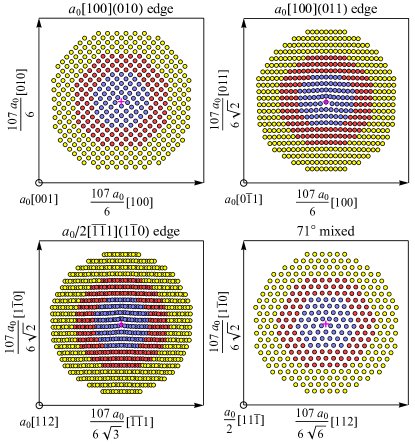
Figure 1: (color online). Initial supercell geometries for the $a_{0}[100](010)$ edge, $a_{0}[100](011)$ edge, $a_{0}/2[\bar{1}\bar{1}1](1\bar{1}0)$ edge, and $a_{0}/2[111](1\bar{1}0)$ $71^{\circ}$ mixed dislocations in bcc Fe. The lattice parameter $a_{0}=2.832$ Å, and the supercell dimensions perpendicular to the dislocation threading direction are 50.46 Å. The atoms are displaced according to anisotropic elasticity theory and divided into three regions to apply FBC. The magenta “+” marks the center of the elastic displacement field. The atoms are surrounded by a vacuum region in all four cases since the dislocation displacement fields are incompatible with periodic boundary conditions. Each supercell is subject to periodic boundary conditions along the threading direction. Table 1 provides more details about the dislocation geometries.

Table 1: Geometry information for the $a_{0}[100](010)$ edge, $a_{0}[100](011)$ edge, $a_{0}/2[\bar{1}\bar{1}1](1\bar{1}0)$ edge, and $a_{0}/2[111](1\bar{1}0)$ $71^{\circ}$ mixed dislocations in bcc Fe. The table lists the number of atoms and the radius in Å of region 1 (blue atoms in Fig. 1), region 2 (red atoms in Fig. 1), and region 3 (yellow atoms in Fig. 1). The radius of each region is nearly equal for each dislocation, but the number of atoms in each region varies between the dislocations due to the different slab thicknesses along the dislocation threading direction.

	region 1		region 2		region 3
dislocation	atoms	radius	atoms	radius	atoms	radius
$a_{0}[100](010)$ edge	60	8.8	110	14.7	216	22.4
$a_{0}[100](011)$ edge	82	8.7	150	14.6	300	22.9
$a_{0}/2[\bar{1}\bar{1}1](1\bar{1}0)$ edge	142	8.7	261	14.5	514	21.8
$a_{0}/2[111](1\bar{1}0)$ $71^{\circ}$ mixed	52	8.8	96	14.8	190	22.4

The FBC approach Sinclair et al. (1978); Woodward (2005) couples the highly distorted dislocation core to an infinite harmonic bulk which effectively allows a dislocation to relax as an isolated defect. The FBC approach consists of two steps: in the first step we use a conjugate gradient optimization scheme with DFT-computed forces to relax the defect core (region 1), while holding the rest of the atoms fixed. This reduces the forces in region 1 but induces forces in region 2. In the second step, we apply displacements on all atoms in regions 1, 2 and 3 in response to the forces in region 2, as prescribed by the LGF $G$,

$$\mathbf{u}(\mathbf{R}^{\prime})=\sum_{\mathbf{R}}G(\mathbf{R}-\mathbf{R}^{\prime})\mathbf{f}(\mathbf{R}),$$ (2)

where $\mathbf{u}(\mathbf{R}^{\prime})$ is the displacement vector of the atom at $\mathbf{R}^{\prime}$ and $\mathbf{f}$ is the Hellmann-Feynman force on the atom at $\mathbf{R}$. The LGF is the pseudoinverse of the force constant matrix $D$ Trinkle (2008),

$$\sum_{\mathbf{R}^{\prime\prime}}D(\mathbf{R}-\mathbf{R}^{\prime\prime})G(\mathbf{R}^{\prime\prime}-\mathbf{R}^{\prime})=\mathbf{1}\delta(\mathbf{R}-\mathbf{R}^{\prime}),$$ (3)

where the force constant matrix element $D_{ab}$ between the atoms at $\mathbf{R}$ and $\mathbf{R}^{\prime}$ is

$$D_{ab}(\mathbf{R}-\mathbf{R}^{\prime})=\left.\frac{\partial^{2}U^{\mathrm{total}}}{\partial u_{a}(\mathbf{R})\partial u_{b}(\mathbf{R}^{\prime})}\right|_{\mathbf{u}=0}.$$ (4)

Here $U^{\mathrm{total}}$ is the total potential energy of the crystal, and $u_{a}$ and $u_{b}$ are Cartesian components of the displacement vectors. The displacements given by the LGF describe the response of an infinite harmonic system; since our system deviates from this harmonic approximation particularly in the dislocation core, this generates forces in region 1. Therefore, we alternate between these two steps until all forces in regions 1 and 2 are smaller than a defined tolerance. We use an efficient numerical method developed in Ref. Tan and Trinkle (2016) to compute the LGFs from the force constants in the dislocated geometries. The force constant and LGF calculations are discussed in the following paragraphs, and the details of the DFT calculations are discussed in Section II.2.

We compute the force constants for the $a_{0}[100](010)$ edge, $a_{0}[100](011)$ edge, and $a_{0}/2[111](1\bar{1}0)$ $71^{\circ}$ mixed dislocations using the bulk-like approximation described in Ref. Tan and Trinkle (2016). We use the small displacement method Kresse et al. (1995); Alfè et al. (2001); Alfè (2009) to compute the force constants of perfect bulk bcc Fe (see Sec. II.2 for details). We then approximate the force constants between pairs of atoms in the dislocation geometries by assigning to them the force constants from the pair of atoms in the bulk which have the closest equivalent pair vector. We have found that this simple approximation works well for most dislocations in simple crystal structures since the force constants are short-ranged and the local environment of atoms appears bulk-like even close to the core Tan and Trinkle (2016).

We use a Gaussian approximation potential (GAP) for bcc Fe Dragoni et al. (2018) to compute the force constants for the $a_{0}/2[\bar{1}\bar{1}1](1\bar{1}0)$ edge dislocation. For this dislocation, the bulk-like approximation failed to produce adequate force constants. This appears to be due to atoms in the initial dislocation core geometry being too close, making it difficult to correctly determine the appropriate pairs of atoms in the bulk corresponding to pairs of atoms in the dislocation. Therefore, we compute the force constant matrix for this dislocation using a finite-difference scheme on each atom in the dislocation geometry to compute derivatives in forces. Since it is prohibitively expensive to do so with DFT, we instead use the Fe GAP to compute the dislocation force constants. The GAP method Bartók et al. (2010) generates classical interatomic potentials that accurately interpolate the potential energy surface of a material using highly flexible basis functions called “smooth overlap of atomic positions” (SOAP) kernels. The SOAP kernels can represent a large range of different local atomic environements that can be encountered during atomistic simulations, and the accuracy and transferability of GAP steps from fitting the SOAP coefficients to a large set of DFT energies, forces, and virials that capture the potential energy surface. We chose the GAP potential for computing the large number of force constants in the $a_{0}/2[\bar{1}\bar{1}1](1\bar{1}0)$ edge dislocation geometry since it provides a good balance between accuracy and speed—while orders of magnitude slower than EAM or MEAM, GAP is still much faster than DFT and can provide accuracy comparable to DFT for computing the properties of bcc Fe Dragoni et al. (2018). We check that the GAP accurately reproduces the lattice and elastic properties from DFT, which is important to ensure consistency between the DFT and LGF relaxations. The GAP lattice constant for bcc Fe is $a_{0}$ = 2.834 Å and the elastic constants are $C_{11}=285.9$ GPa, $C_{12}=154.3$ GPa and $C_{44}=103.8$ GPa, which agree well with our DFT-computed lattice constant of $a_{0}$ = 2.832 Å and elastic constants $C_{11}=277.5$ GPa, $C_{12}=147.7$ GPa and $C_{44}=98.1$ GPa Fellinger et al. (2017). In addition, we check that the force constants from the GAP agree well with the force constants from DFT. Figure 2 compares the DFT and GAP force constants computed for bulk bcc Fe under different volumetric strains $e_{V}$. The maximum absolute errors between the GAP and DFT force constants occur for the on-site term $(r=0)$, which correspond to relative errors of less than 3% for all three strain values, $e_{V}=-5$%, $e_{V}=0$% and $e_{V}=+5$%. Therefore, we expect the GAP to predict force constants in the strained dislocation geometries which are consistent with DFT.

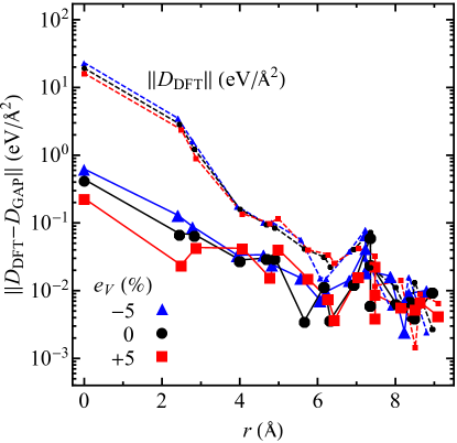
Figure 2: (color online). Difference between the DFT and GAP force constants versus distance $r$ between pairs of atoms for different volumetric strains $e_{V}$. For each value of $r$ we take the Frobenius norm of the difference between the DFT and GAP force constant matrices $D$. The dashed lines show $||D_{\mathrm{DFT}}||$ for each value of strain. The force constants decay as $r$ increases and the differences show similar behavior. The maximum difference for each strain occurs at $r=0$ (i.e., the on-site term), where $||D_{\mathrm{DFT}}||=19.273$ eV/Ų and $||D_{\mathrm{GAP}}||=19.713$ eV/Ų for $e_{V}=0$. The corresponding relative error is 2.28%, with similar maximum errors for $e_{V}=-5$% (2.69% error) and $e_{V}=+5$% (1.42% error).

We numerically invert the dislocation force constant matrices following the method developed in Ref. Tan and Trinkle (2016). This method requires setting up a large system divided into five regions: regions 1, 2, and 3 which make up the DFT supercell, a buffer region, and a far-field region. The far-field region contains atoms far away from the core whose displacements we approximate using the bulk elastic Green function (EGF) which is the known large distance limit of the LGF Trinkle (2008); Yasi and Trinkle (2012), while the buffer region contains the remaining atoms between region 3 and the far-field. For all the dislocations studied here, we used a buffer size of at least $20a_{0}$, for which the errors in the LGF computation due to the far-field approximation are on the order of $10^{-3}\textrm{\AA}^{2}$/eV or less. We compute the LGF for forces in region 2 by applying a unit force on an atom in region 2, evaluating the resulting far-field displacements based on the EGF, determining the forces these displacements generate in the buffer region, and finally solving for the displacement field corresponding to the effective forces in the system by using a conjugate gradient method to numerically invert the force constant matrix. This gives one column of the LGF; by systematically looping through every atom in region 2, we compute the LGF matrix that gives displacements on atoms in regions 1, 2, and 3 due to forces in region 2. For more details on this method, the reader is referred to Ref. Tan and Trinkle (2016).

II.2 Density functional theory calculation details

We use the plane-wave basis DFT code vasp Kresse and Furthmüller (1996) to generate data for computing bulk force constants and to optimize the geometries of the edge and mixed dislocations in bcc Fe. The Perdew-Burke-Ernzerhof (PBE) generalized gradient approximation (GGA) functional Perdew et al. (1996) accounts for electron exchange and correlation energy, and a projector augmented wave (PAW) potential Blöchl (1994) with electronic configuration [Ar]$3d^{7}4s^{1}$ generated by Kresse and Joubert Kresse and Joubert (1999) models the Fe nuclei and core electrons. The calculations require a plane-wave energy cutoff of 400 eV to converge the energies to less than 1 meV/atom. We ensure accurate forces for force constant calculations and atomic relaxation using Methfessel-Paxton smearingMethfessel and Paxton (1989) with an energy smearing width of 0.25 eV. We chose this smearing width to ensure close agreement between the smeared electronic density of states (DOS) of bulk bcc Fe near the Fermi energy and the DOS computed using the linear tetrahedron method with Blöchl corrections Blöchl et al. (1994). The energy tolerance for the electronic self-consistency cycle is $10^{-8}$ eV. All of the calculations are spin polarized to model the ferromagnetism of bcc Fe.

We use the small displacement method Kresse et al. (1995); Alfè et al. (2001); Alfè (2009) to compute the force constants of bulk bcc Fe used in the bulk-like approximation of the dislocation force constants (see Sec. II.1). To ensure that the LGFs computed from the force constants match the elastic Green function in the limit ${\mathbf{R}}\rightarrow\infty$, the elastic constants $C_{ijkl}$ computed from the bulk force constant matrix $D_{ij}({\mathbf{R}})$ must match the elastic constants computed using standard stress-strain calculations Trinkle (2008). The elastic constants $C_{ijkl}$ of a crystal with a single basis atom can be computed from the force constant matrix $D_{ij}({\mathbf{R}})$ using the method of long waves Trinkle (2008); Born and Huang (1954),

$$-\sum_{\mathbf{R}}D_{ij}({\mathbf{R}})R_{k}R_{l}=V_{0}\left(C_{ikjl}+C_{iljk}\right),$$ (5)

where $V_{0}$ is the volume of the primitive cell. However, numerical errors in the DFT forces between pairs of atoms with large ${\mathbf{R}}$ can compound to produce large errors in the $C_{ijkl}$. We examine the effect of supercell size on the errors in the force constants and the corresponding computed $C_{ijkl}$ by performing small displacement method calculations using $3\times 3\times 3$, $4\times 4\times 4$, $5\times 5\times 5$, and $6\times 6\times 6$ supercells with $10\times 10\times 10$, $8\times 8\times 8$, $6\times 6\times 6$, and $6\times 6\times 6$ $\Gamma$-centered Monkhorst-Pack $k$-point meshesMonkhorst and Pack (1976), respectively. In all these calculations, the atom at the origin of the supercell was given a displacement of 0.02 Å along a supercell lattice vector and the resulting forces were input into the code phon Alfè (2009) to compute the force constants. We find that the force constants computed using the $4\times 4\times 4$ supercell produce $C_{ijkl}$ values closest to the $C_{ijkl}$ from stress-strain calculations Fellinger et al. (2017), but the values differ by up to 25 GPa. We therefore computed the force constants of bulk bcc Fe using the force data from the $4\times 4\times 4$ supercell calculation under the constraint that the sum in Eqn. 5 gives $C_{ijkl}$ values that exactly match the $C_{ijkl}$ from our stress-strain calculations. These constrained force constants are used in the bulk-like approximation of the force constants for the $a_{0}[100](010)$ edge, $a_{0}[100](011)$ edge, and $a_{0}/2[111](1\bar{1}0)$ $71^{\circ}$ mixed dislocations. Figure 2 compares the unconstrained force constants under volumetric strain computed with GAP and DFT using $6\times 6\times 6$ supercells. Force constants computed using classical potentials like GAP are not subject to the same types of numerical error as the DFT force constants, so we do not constrain the GAP force constants computed directly for the $a_{0}/2[\bar{1}\bar{1}1](1\bar{1}0)$ edge dislocation (see Sec. II.1).

We use DFT with FBC to relax the atoms in regions 1 and 2 of the edge and mixed dislocation geometries. We sample the Brillouin zones of the dislocation supercells using $1\times 1\times 18$, $1\times 1\times 14$, $1\times 1\times 8$, and $1\times 1\times 20$ $\Gamma$-centered Monkhorst-Pack meshes for the $a_{0}[100](010)$ edge, $a_{0}[100](011)$ edge, $a_{0}/2[\bar{1}\bar{1}1](1\bar{1}0)$ edge, and $a_{0}/2[111](1\bar{1}0)$ $71^{\circ}$ mixed dislocations, respectively. We relax the atoms in regions 1 and 2 of the $a_{0}[100](010)$ edge, $a_{0}[100](011)$ edge, and $a_{0}/2[111](1\bar{1}0)$ $71^{\circ}$ mixed dislocation geometries until the forces on the ions are less than 5 meV/Å. Due to the larger computational cost of relaxing the $a_{0}/2[\bar{1}\bar{1}1](1\bar{1}0)$ edge dislocation, we relax the atoms in regions 1 and 2 of this dislocation until all of the forces on the ions are less than 18 meV/Å. We compared the final relaxed core structures of the other dislocations to their core structures earlier in their relaxation when the largest forces were $\sim 18$ meV/Å, and found negligible differences in the geometries; therefore, we consider the $a_{0}/2[\bar{1}\bar{1}1](1\bar{1}0)$ edge dislocation core structure to effectively be fully optimized by that point in the relaxation.

II.3 Dislocation core visualization

We visualize the relaxed core structures of the dislocations using a combination of differential displacement (DD) maps Vítek et al. (1970), Nye tensor components $\alpha_{jk}$ Hartley and Mishin (2005a, b), volumetric strain $e_{V}$, and changes in the local magnetic moments $m$ on the Fe atoms. The DD maps display the core structure of a dislocation as arrows that indicate the relative displacements between pairs of atoms. The Nye tensor components $\alpha_{jk}$ represent the local Burgers vector density at each site in the dislocation core, where the first index $j$ corresponds to the dislocation threading direction and the second index $k$ specifies the Cartesian component of the local Burgers vector at each site. For the dislocations in this study, the only non-zero Nye tensor components are $\alpha_{3k}$ since the threading direction of each dislocation is chosen along the $z$-axis. We visualize the Nye tensor distributions as linearly interpolated contour plots. The dislocations strain the lattice, and magnetostrictive materials such as Fe show changes in magnetism under strain du Tremolet de Lacheisserie and Monterroso (1983). The dislocation strain fields and the corresponding local changes in the magnetic moments on the Fe atoms give a complementary view of the core structures.

We define the centers and widths of the dislocation cores as the first and second moments of the Nye tensor distributions. We define the normalized Nye tensor components $\widetilde{\alpha}_{3k}$ as

$$\widetilde{\alpha}_{3k}(x,y):=\frac{|\alpha_{3k}(x,y)|}{\sum_{x^{\prime},y^{\prime}}|\alpha_{3k}(x^{\prime},y^{\prime})|},$$ (6)

where $(x,y)$ is the coordinates of a site in the plane normal to the dislocation threading direction. The first moments $\overline{x}_{3k}$ and $\overline{y}_{3k}$ of the normalized Nye tensor components,

$$\begin{split}\overline{x}_{3k}&:=\sum_{x,y}x\,\widetilde{\alpha}_{3k}(x,y),\\ \overline{y}_{3k}&:=\sum_{x,y}y\,\widetilde{\alpha}_{3k}(x,y),\end{split}$$ (7)

define the center of each $\alpha_{3k}$ distribution. The second moments $\sigma_{3k,x}$ and $\sigma_{3k,y}$ of the normalized Nye tensor components,

$$\begin{split}\sigma^{2}_{3k,x}&:=\sum_{x,y}\left(x-\overline{x}_{3k}\right)^{2}\widetilde{\alpha}_{3k}(x,y),\\ \sigma^{2}_{3k,y}&:=\sum_{x,y}\left(y-\overline{y}_{3k}\right)^{2}\widetilde{\alpha}_{3k}(x,y),\end{split}$$ (8)

give the widths of a Nye tensor distribution.

We compute Fourier coefficients of the Nye tensor distributions to quantify the symmetry differences between the dislocation core structures computed using DFT and the core structures computed using different classical potentials. The $p^{\mathrm{th}}$ Fourier coefficient $c_{3k,p}$ of each $\alpha_{3k}$ about the center $(\overline{x}_{3k},\overline{y}_{3k})$ is

$$c_{3k,p}:=\sum_{x,y}\alpha_{3k}(x,y)e^{-ip\theta(x,y)},$$ (9)

where $\theta(x,y):=\arctan\left[(y-\overline{y}_{3k})/(x-\overline{x}_{3k})\right]$ is the angular coordinate of a site $(x,y)$. The $c_{3k,p}$ quantify the $p$-fold rotational symmetry content of the Nye tensor distributions.

Lastly, we compute the local volumetric strain at each site near the dislocation cores using Yasi et al. (2010)

$$e_{V}:=\left[\frac{\mathrm{det}\big{\{}\sum_{\mathbf{v^{\prime}}}v^{\prime}_{j}v^{\prime}_{k}\big{\}}}{\mathrm{det}\big{\{}\sum_{\mathbf{v}}v_{j}v_{k}\big{\}}}\right]^{1/2}-1,$$ (10)

where $\mathbf{v^{\prime}}$ are the nearest neighbor vectors of an atom in the dislocation geometry, $\mathbf{v}$ are the corresponding nearest neighbor vectors in bulk, and $j$ and $k$ denote Cartesian components. Since the strain is computed at discrete sites like the Nye tensor components, we visualize the strain distributions as linearly interpolated contour plots.

III Results

III.1 Dislocation core structures: First-principles calculations

Figures 3–5 show that the DFT-optimized core structures of the edge dislocations are compact and the magnetic moments on the atoms above (below) the slip planes decrease (increase) due to the volumetric strain fields around the dislocation cores. The $\alpha_{32}$ and $\alpha_{33}$ distributions are nearly zero for the $a_{0}[100](011)$ and $a_{0}/2[\bar{1}\bar{1}1](1\bar{1}0)$ edge dislocations, but unexpectedly we find that $\alpha_{32}$ is about one-half as large as $\alpha_{31}$ for the $a[100](010)$ edge dislocation. The $x$- and $y$-directions for the $a[100](010)$ dislocation are both $\langle 100\rangle$-type directions, and we surmise that it is more energetically favorable to displace in the $y$-direction compared to the other two edge dislocations. Separately, we have optimized the core structure of the $a_{0}/2[111]$ screw dislocation in bcc Fe using FBC Fellinger et al. (2018). The relaxed core structure is symmetric and compact like in other bcc metals Ismail-Beigi and Arias (2000); Woodward and Rao (2001, 2002); Frederiksen and Jacobsen (2003); Ventelon et al. (2013); Dezerald et al. (2015), and we compute the widths of the core as $2\sigma_{33,x}=3.20$ Å and $2\sigma_{33,y}=3.25$ Å. Table 2 shows that the widths of the edge dislocation cores are similar to the widths of the screw dislocation core, confirming that the edge dislocation cores remain compact after relaxation. The $\alpha_{31}$ and $\alpha_{32}$ distributions of the $a_{0}[100](010)$ edge dislocation go to zero at similar distances from their centers, but $\alpha_{32}$ has a larger $x$ width since it is antisymmetric. The fourth panels in Figures 3–5 illustrates the magnetostrictive effect in the dislocation cores—compressive strain reduces magnetization and tensile strain increases magnetization. We initialize the magnetic moments for all four dislocations in this study in a ferromagnetic state with equal moment values. The relaxed moment values decrease or increase based on the local strain distribution, but the ordering remains ferromagnetic throughout all four geometries. We further explore the changes in magnetic moments later in this section (see Figure 7).

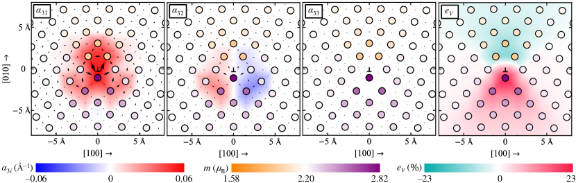
Figure 3: (color online). Core structure of the $a_{0}[100](010)$ edge dislocation in bcc Fe. The first three panels show the differential displacement maps using black arrows and the Nye tensor components $\alpha_{3i}$ as contour plots (blue to red color scale). The $\alpha_{31}$ and $\alpha_{32}$ distributions reflect the edge character of the dislocation, and the $\alpha_{33}$ distribution reflects the screw character. The fourth panel shows the volumetric strain $e_{V}$ as a contour plot (cyan to magenta color scale). The atoms in all four panels are colored based on their magnetic moments $m$ (orange to purple color scale). The core has edge character in both the $x$- and $y$-directions and it remains compact after relaxation. The screw component $\alpha_{33}$ of the dislocation is zero. The magnetic moments on the Fe atoms decrease in the compressive region above the slip plane and increase in the tensile region below the slip plane.

Table 2: Widths of the Nye tensor distributions $\alpha_{3k}$ for the edge and mixed dislocations in bcc Fe. We define the widths of $\alpha_{3k}$ in the $x$- and $y$-directions as two times the corresponding second moment computed using Eqn. 8. The edge and mixed cores are compact since their widths are comparable to the widths of $\alpha_{33}$ for the ${a_{0}}/2[111]$ screw dislocation in bcc Fe ($x$ width = 3.20 Å and $y$ width = 3.25 Å).

dislocation, $\alpha_{3k}$	$x$ width (Å)	$y$ width (Å)
$a_{0}[100](010)$ edge, $\alpha_{31}$	3.78	3.92
$a_{0}[100](010)$ edge, $\alpha_{32}$	4.69	3.04
$a_{0}[100](011)$ edge, $\alpha_{31}$	4.31	3.38
$a_{0}/2[\bar{1}\bar{1}1](1\bar{1}0)$ edge, $\alpha_{31}$	4.33	3.00
$a_{0}/2[111](1\bar{1}0)$ $71^{\circ}$ mixed, $\alpha_{31}$	3.97	3.28
$a_{0}/2[111](1\bar{1}0)$ $71^{\circ}$ mixed, $\alpha_{33}$	4.41	3.30

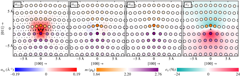
Figure 4: (color online). Core structure of the $a_{0}[100](011)$ edge dislocation in bcc Fe. Similar to the $a_{0}[100](010)$ edge dislocation, the core is compact, the screw component is zero, and the magnetic moments decrease(increase) if the atoms are above(below) the slip plane due to the dislocation strain field. The edge component of this dislocation in the $y$-direction is nearly zero.

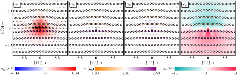
Figure 5: (color online). Core structure of the $a_{0}/2[\bar{1}\bar{1}1](1\bar{1}0)$ edge dislocation in bcc Fe. Similar to the $a_{0}[100](010)$ and $a_{0}[100](011)$ edge dislocations, the relaxed core is compact, the screw component is zero, and the magnetic moments increase(decrease) in response to compressive(tensile) strains in the core. The edge component of this dislocation in the $y$-direction is nearly zero.

Figure 6 shows that the DFT-optimized core structure of the $a_{0}/2[111](1\bar{1}0)$ $71^{\circ}$ mixed dislocation is compact and the changes in the magnetic moments on the atoms near the core reflect the volumetric strain field of the edge component. The Burgers vector and threading direction for the mixed dislocation are along two different body-diagonals of the cubic unit cell, separated by an angle of $\approx 71^{\circ}$. Hence, the edge component $\alpha_{31}$ of the dislocation is larger than the screw component $\alpha_{33}$ as shown in Figure 6. The edge component perpendicular to the Burgers vector $(\alpha_{32})$ is nearly zero. Similar to the edge dislocations, the magnetic moments on atoms above the slip plane are reduced from their bulk values due to compressive strain and the moments on the atoms below the slip plane are enhanced due to tensile strain. This is primarily due to the volumetric strain field generated by the edge component of the dislocation (see Fig. 7), since the volumetric strain induced by the screw component is small.

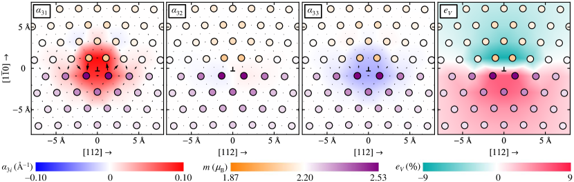
Figure 6: (color online). Core structure of the $a_{0}/2[111](1\bar{1}0)$ $71^{\circ}$ mixed dislocation in bcc Fe. In this case, the dislocation has both edge ($\alpha_{31}$) and screw ($\alpha_{33}$) components due to its mixed character. Since the volumetric strain due to the screw component is small, the changes in the magnetic moments of the Fe atoms are largely due to the edge component of the dislocation. The dislocation core is compact after relaxation like the edge dislocation cores.

Figure 7 shows that the magnetic moments around the dislocation cores closely follow the magnetic moments in bulk bcc Fe for small volumetric strains but deviate for the larger strains found in the cores. We use the average nearest-neighbor distance as an alternative measure of local volumetric strain since it better correlates the magnetic moments near the dislocations with the moments in strained bulk. For reference, the average nearest-neighbor distance in unstrained bulk bcc Fe is $\sqrt{3}a_{0}/2=2.453$ Å. We compute the bulk magnetic moments by applying different volumetric strains to the bcc unit cell. However, each dislocation is under a different strain condition since the normal strain along their different threading directions is zero. We have also computed the variation in magnetization of bulk bcc Fe under the different strain conditions corresponding to each dislocation and found that the behavior is nearly identical to the volumetric strain dependence for the strain range shown in the figure. We find that the magnetic moments on the atoms in the dislocations closely follow the magnetic moments in strained bulk for sites with about $-2\%$ to $+5\%$ local volumetric strain. The outlying data points correspond to atoms right in the dislocation cores where the local strains are larger and non-volumetric contributions to strain may become important.

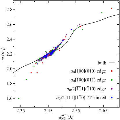
Figure 7: (color online). Local magnetic moments $m$ near the dislocation cores versus average nearest-neighbor distance $d^{\mathrm{avg}}_{\mathrm{NN}}$. The discrete points are the values for the magnetic moments near the dislocation cores and the solid line show the variation of the magnetic moment of bulk bcc Fe versus nearest-neighbor distance. The average nearest-neighbor distance is an alternative measure of local volumetric strain which better correlates the magnetic moments near the dislocations with the moments in strained bulk, especially for the large strains found in the dislocation cores. The average nearest-neighbor distance in unstrained bulk bcc Fe is $d^{\mathrm{avg}}_{\mathrm{NN}}=2.453$ Å.

III.2 Dislocation core structures: Comparison of interatomic potentials to DFT

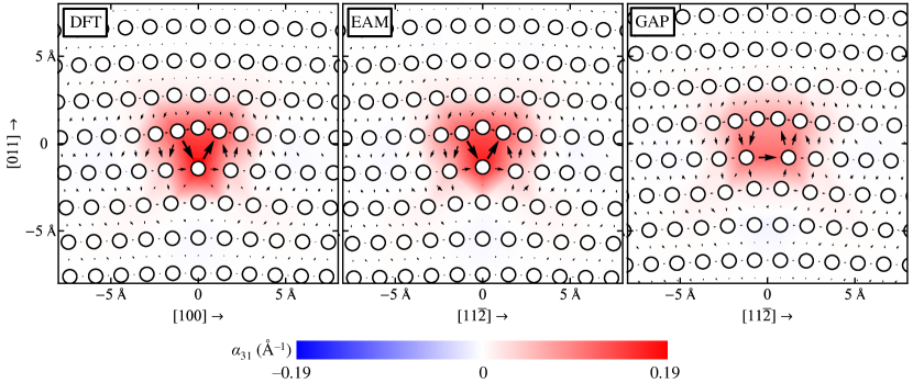
Figure 9: (color online). Comparison of DFT, EAM Mendelev et al. (2003), and GAP Dragoni et al. (2018) results for the core structure of the $a_{0}[100](011)$ edge dislocation. The figures show the $\alpha_{31}$ edge component of the Nye tensor, and the atoms in this DFT figure are not colored based on their magnetic moments. The EAM potential produces a core structure similar to DFT, but the GAP core is different. This is reflected by the large differences between the DFT and GAP Fourier coefficients in Fig. 8

Figure 8 compares the DFT core structures of the edge and mixed dislocations to the cores from GAP Dragoni et al. (2018), MEAM Asadi et al. (2015), and EAM Ackland et al. (1997); Ramasubramaniam et al. (2009); Malerba et al. (2010); Marinica et al. (2012); Mendelev et al. (2003); Chamati et al. (2006); Proville et al. (2012) potentials using the Fourier coefficients $c_{3k,p}$ of the Nye tensor distributions. The classical potential calculations are performed using the code lammps Plimpton (1995), with potential parameters downloaded from the NIST Interatomic Potential Repository NIS (2018) with the exception of Ref. Ramasubramaniam et al. (2009) EAM, which used the recommended PotentialB.fs file downloaded from Ref. car (2017). The supercells in the classical potential calculations contain cylindrical slab geometries with approximately 20,000 atoms surrounded by vacuum. We use fixed boundary conditions where the atoms at a distance less than the potential cutoff radii from the vacuum are held at their positions from anisotropic elasticity theory while all the other atoms are relaxed using a conjugate gradient method. The $c_{3k,p}$ (see Eqn. 9) quantify the differences in the $p$-fold symmetry content between the dislocation cores computed using different methods. For example, the core of the $a_{0}[100](011)$ edge dislocation relaxes to a different structure than the DFT core using the GAP and there are large difference between the GAP and DFT $c_{31,p}$ for $p>1$. In contrast, the EAM and MEAM $c_{31,p}$ for this dislocation agree well with the DFT values. Figure 9 shows that the core computed using the EAM potential from Ref. Mendelev et al. (2003) is similar to the DFT core, but the GAP core relaxes to a more open structure. We find the largest differences from the DFT core structures when the $a_{0}[100](010)$ edge dislocation is relaxed using the EAM potentials from Refs. Ramasubramaniam et al. (2009); Proville et al. (2012), when the $a_{0}[100](011)$ edge dislocation is relaxed using GAP Dragoni et al. (2018), when the $a_{0}/2[\bar{1}\bar{1}1](1\bar{1}0)$ edge dislocation is relaxed using the EAM potential from Ref. Proville et al. (2012), and when the $a_{0}/2[111](1\bar{1}0)$ $71^{\circ}$ mixed dislocation is relaxed using the MEAM potential Asadi et al. (2015). The study in Ref. S.M. Hafez Haghighat et al. (2014a) found that the EAM potential from Ref. Mendelev et al. (2003) produces a different core structure for $a_{0}/2\langle 111\rangle\{110\}$ edge dislocations compared to the EAM potentials in Refs. Ackland et al. (1997); Malerba et al. (2010); Marinica et al. (2012), whereas we find that all of these potentials produce core structures similar to our DFT core. We are able to reproduce the core structures in Ref. S.M. Hafez Haghighat et al. (2014a) by choosing different elastic centers for the initial dislocation geometry, but these cores transform to the other core after annealing from 300K. We also find that the two types of cores are nearly degenerate in energy which is consistent with the nudged elastic band calculations in Ref. S.M. Hafez Haghighat et al. (2014a), so it is likely that the core we found is the ground state structure and the other core is a transition state as the dislocation moves in its slip plane.

The alternate structure of the $a_{0}/2[\bar{1}\bar{1}1](1\bar{1}0)$ edge dislocation for the EAM potential from Ref. Mendelev et al. (2003) discussed in the last paragraph raises the question about the existence of metastable states for the other dislocation cores considered in this study. Metastable core structures are most likely for dislocations with large spreading in the slip plane or that dissociate into partial dislocations separated by stacking fault since multiple energy minimia are present in the slip plane. We do not expect metastable core structures to exist for the dislocations in this study since all the DFT cores are compact. We invesitagate this idea further by annealing the cores from the EAM and MEAM potentials that are most similar to the DFT cores to examine if these structures are stable. We anneal the $a_{0}[100](010)$ edge dislocation cores for the EAM potentials from Refs. Ackland et al. (1997); Mendelev et al. (2003) and the MEAM potential, the $a_{0}[100](011)$ edge cores for the EAM potentials from Refs. Ackland et al. (1997); Ramasubramaniam et al. (2009); Malerba et al. (2010); Marinica et al. (2012); Mendelev et al. (2003); Chamati et al. (2006) and the MEAM potential, the $a_{0}/2[\bar{1}\bar{1}1](1\bar{1}0)$ edge cores for the EAM potentials from Refs. Ackland et al. (1997); Ramasubramaniam et al. (2009); Malerba et al. (2010); Marinica et al. (2012); Mendelev et al. (2003); Chamati et al. (2006) and the MEAM potential, and the mixed cores for the EAM potentials from Refs. Ackland et al. (1997); Ramasubramaniam et al. (2009); Malerba et al. (2010); Marinica et al. (2012); Mendelev et al. (2003); Chamati et al. (2006). In each case, the initial geometry for the annealing simulation is the conjugate gradient-optimized geometry with Fourier coefficients shown in Figure 8. We anneal the cores from a starting temperature of 300K and then perform a subsequent conjugate gradient geometry optimization. All of the annealed core structures remain unchanged except for the $a_{0}[100](010)$ edge dislocation from the EAM potential in Ref. Mendelev et al. (2003) which remains compact but becomes asymmetric in the slip direction, the $a_{0}[100](011)$ edge dislocation from the MEAM potential which has a larger spreading in the slip plane than the initial structure, and the mixed dislocation from the EAM potential in Ref. Ackland et al. (1997) which transforms to a structure similar to the MEAM structure. The GAP cores of the $a_{0}[100](010)$ edge, $a_{0}/2[\bar{1}\bar{1}1](1\bar{1}0)$ edge, and $a_{0}/2[111](1\bar{1}0)$ $71^{\circ}$ mixed dislocations are similar to the DFT cores. GAP calculations are more computationally expensive than EAM and MEAM calculations, so we only annealed the GAP mixed dislocation core. For the two GAP edge dislocations that are similar to DFT we applied small random displacements to the atoms in the core region and then relaxed the geometry using a conjugate gradient method. All three GAP dislocation cores relax back to their starting geometries. Finally, we investigated the stability of the DFT mixed dislocation geometry by performing restoring force calculations. We added small displacements along the slip direction to the four atoms directly above the slip plane that are closest to the center of the dislocation core, and computed the resulting forces using DFT. The forces primarily point opposite to the displacement direction, indicating that the core will relax back to the original geometry. All of these test calculations strongly suggest that the DFT core structures reported in this study are stable groundstate structures, and that the core transformations we find after annealing are due to artifacts in the interatomic potentials. None of the potentials is able to produce core geometries similar to DFT for all of the dislocations, but the EAM potential from Ref. Mendelev et al. (2003) has the best overall performance. All of the core geometries optimized with this potential using a conjugate gradient method are similar to DFT, and they all remain stable under annealing except for the $a_{0}[100](010)$ edge dislocation which breaks symmetry but remains compact. This EAM potential also produces a compact and symmetric core structure for $a_{0}/2\langle 111\rangle$ screw dislocations similar to DFT Malerba et al. (2010).

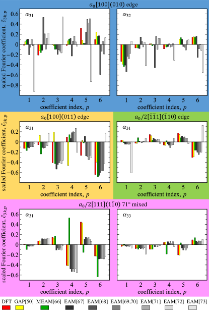
Figure 8: (color online). Fourier coefficients of the Nye tensors computed using DFT and GAP Dragoni et al. (2018), MEAM Asadi et al. (2015), and EAM Ackland et al. (1997); Ramasubramaniam et al. (2009); Malerba et al. (2010); Marinica et al. (2012); Mendelev et al. (2003); Chamati et al. (2006); Proville et al. (2012) potentials. The coefficients with even indices are real and the coefficients with odd indices are imaginary. We show only the coefficient values for positive indices since the negative even coefficients equal the positive even coefficients, and the negative odd coefficients have equal magnitudes and opposite signs as the positive odd coefficients. The scaled coefficients in the figure are defined as ${\widetilde{c}}_{3k,p}=c_{3k,p}/c_{31,0}$. The plots reveal the differences in symmetry between the cores, and can be used to quickly judge if a given potential produces a core structure similar to DFT. For example, the GAP cores of the $a_{0}[100](010)$ edge, $a_{0}/2[\bar{1}\bar{1}1](1\bar{1}0)$ edge, and $a_{0}/2[111](1\bar{1}0)$ $71^{\circ}$ mixed dislocation agree well with DFT, but the GAP core of the $a_{0}[100](011)$ edge dislocation relaxes to a more open structure (see Fig. 9 for a direct comparison of the cores).

.

IV Summary and discussion

We use density functional theory (DFT) with lattice flexible boundary conditions (FBC) to optimize the core structures of $a_{0}[100](010)$ edge, $a_{0}[100](011)$ edge, $a_{0}/2[\bar{1}\bar{1}1](1\bar{1}0)$ edge, and $a_{0}/2[111](1\bar{1}0)$ $71^{\circ}$ mixed dislocations in bcc Fe. The FBC approach couples the highly-distorted dislocation core which is treated with DFT to an infinite harmonic lattice via the lattice Green function (LGF), which allows the dislocation to effectively relax as an isolated defect. In contrast to most previous first-principles FBC calculations of dislocation cores that use the bulk LGF to relax the harmonic region outside the core, we use LGFs specifically computed for each dislocation geometry. The simple bulk-like approximation we used for generating the force constants and corresponding LGFs for the $a_{0}[100](010)$ edge, $a_{0}[100](011)$ edge, and $a_{0}/2[111](1\bar{1}0)$ $71^{\circ}$ mixed dislocations fails to produce an adequate LGF for the $a_{0}/2[\bar{1}\bar{1}1](1\bar{1}0)$ edge dislocation. For this case, we found that a Gaussian approximation potential (GAP) for bcc Fe produces accurate force constants under strain which lead to a dislocation LGF capable of optimizing the core geometry. We find that the cores of all the dislocations in this study are compact and the magnetic moments on the atoms in the cores increase in the tensile region below the slip planes and decrease in the compressive region above the slip planes. Except for highly distorted sites nearest to the cores, the strain response of the magnetic moments on the atoms in the dislocated geometries closely follows the volumetric-strain response of the magnetic moment in bulk bcc Fe. We find that the initial ferromagnetic ordering we impose on the magnetic moments in each geometry remains after relaxation, showing that ferromagnetic ordering in the cores is at least metastable. Future studies could investigate the impact of different initial magnetic configurations in the dislocation cores on their relaxed magnetic states and geometries. We find that most of the core structures computed using the GAP, MEAM, and EAM interatomic potentials compare well with the DFT core structures, with a few notable exceptions where the cores relax to different structures. While none of the potentials is able to produce core geometries similar to DFT for all of the dislocations, the EAM potential from Ref.Mendelev et al. (2003) has the best overall performance. All of the core geometries optimized with this potential using a conjugate gradient method are similar to DFT, and they all remain stable under annealing except for the $a_{0}[100](010)$ edge dislocation which remains compact but becomes asymmetric along the slip direction. Additionally, this EAM potential produces a compact and symmetric core structure for $a_{0}/2\langle 111\rangle$ screw dislocations similar to DFTMalerba et al. (2010). Relaxed dislocation core structures are of fundamental importance for understanding plasticity in bcc Fe, provide the geometries required for first principles-based studies of solid-solution strengtheningYasi et al. (2010) and solute diffusion near dislocationsSchiavone and Trinkle (2016), provide data for parameterizing and benchmarking more computationally efficient models such as classical interatomic potentials, and serve as a comparison point for future experimental measurement of edge and mixed dislocation core structures in bcc Fe.

V Data availability

The vasp and lammps input files used to perform the calculations along with the relaxed dislocation core geometries are available to download from http://hdl.handle.net/11256/978.