Concentrated Differentially Private Gradient Descent with Adaptive per-Iteration Privacy Budget

Abstract.

Iterative algorithms, like gradient descent, are common tools for solving a variety of problems, such as model fitting. For this reason, there is interest in creating differentially private versions of them. However, their conversion to differentially private algorithms is often naive. For instance, a fixed number of iterations are chosen, the privacy budget is split evenly among them, and at each iteration, parameters are updated with a noisy gradient.

In this paper, we show that gradient-based algorithms can be improved by a more careful allocation of privacy budget per iteration. Intuitively, at the beginning of the optimization, gradients are expected to be large, so that they do not need to be measured as accurately. However, as the parameters approach their optimal values, the gradients decrease and hence need to be measured more accurately. We add a basic line-search capability that helps the algorithm decide when more accurate gradient measurements are necessary.

Our gradient descent algorithm works with the recently introduced zCDP version of differential privacy. It outperforms prior algorithms for model fitting and is competitive with the state-of-the-art for $(\epsilon,\delta)$-differential privacy, a strictly weaker definition than zCDP.

1. Introduction

Iterative optimization algorithms are designed to find a parameter vector $\bm{\mathrm{w}}^{*}\in\mathbb{R}^{p}$ that minimizes an objective function $f$. They start with an initial guess $\bm{\mathrm{w}}_{0}$ and generate a sequence of iterates $\{\bm{\mathrm{w}}_{t}\}_{t\geq 0}$ such that $\bm{\mathrm{w}}_{t}$ tends to $\bm{\mathrm{w}}^{*}$ as $t\to\infty$. At iteration $t$, information about the objective function $f(\bm{\mathrm{w}}_{t})$, such as the gradient $\nabla f(\bm{\mathrm{w}}_{t})$, is computed and used to obtain the next iterate $\bm{\mathrm{w}}_{t+1}$. In the case of gradient (or stochastic gradient) descent, updates have a form like:

(1) $$\bm{\mathrm{w}}_{t+1}=\bm{\mathrm{w}}_{t}-\alpha_{t}(\nabla f(\bm{\mathrm{w}}_{t}))\,,$$

where $\alpha_{t}$ is a carefully chosen step size that often depends on the data (for example, through a line search (Nocedal and Wright, 2006)) or based on previous gradients.

When designing a such algorithm under various versions of differential privacy, the update steps typically have the following form (Song et al., 2013; Abadi et al., 2016):

(2) $$\bm{\mathrm{w}}_{t+1}=\bm{\mathrm{w}}_{t}-\alpha_{t}(\nabla f(\bm{\mathrm{w}}_{t})+Y_{t})\,,$$

where $Y_{t}$ is an appropriately scaled noise variable (e.g., Laplace or Gaussian) for iteration $t$, and the gradient may be computed on some or all of the data. It is important to note that the noisy gradients $\nabla f(\bm{\mathrm{w}}_{t})+Y_{t}$ might not be descent directions even when computed on the entire dataset.

In prior work (e.g., (Zhang et al., 2013; Bassily et al., 2014; Talwar et al., 2015; Wang et al., 2015)), the total number of iterations $T$ is fixed a priori, and the desired privacy cost, say $\epsilon$, is split across the iterations: $\epsilon=\epsilon_{1}+\dots+\epsilon_{T}$. For any iteration $t$, the variance of $Y_{t}$ is a function of $1/\epsilon_{t}$ and depends on which version of differential privacy is being used (e.g., pure differential privacy (Dwork et al., 2006b), approximate differential privacy (Dwork et al., 2006a), or zero-mean concentrated differential privacy (Bun and Steinke, 2016)). Furthermore, in prior work, the privacy budget is evenly split across iterations, so $\epsilon_{1}=\dots=\epsilon_{T}=\epsilon/T$.

There are two drawbacks to this approach. First, accuracy heavily depends on the pre-specified number of iterations $T$ — if $T$ is too small, the algorithm will stop well short of the optimum; if $T$ is too large, the privacy budget $\epsilon_{t}$ for each iteration is small, so that large amounts of noise must be added to each gradient, thus swamping the signal provided by the gradient. Second, at the beginning of the optimization, gradients are expected to be large, so that an algorithm can find good parameter updates even when the gradient is not measured accurately. However, as the current parameters $\bm{\mathrm{w}}_{t}$ approach the optimal values, the gradients start to decrease and need to be measured more accurately in order for the optimization to continue making progress (e.g., continue to minimize or approximately minimize $f$). This means that an adaptive privacy budget allocation is preferable to a fixed allocation (as long as the total privacy cost is the same).

In this paper, we propose an adaptive gradient descent strategy for zero-mean Concentrated Differential Privacy (Bun and Steinke, 2016) (zCDP) where each iteration has a different share $\epsilon_{t}$ of the overall privacy budget $\epsilon$. It uses a smaller share of the privacy budget (more noise) for gradients with large norm and a larger share (less noise) for gradients with small norm. Thus, if there are many steps with large gradients, the algorithm will be able to run for more iterations, while if there are many steps with small gradients, it will run for fewer iterations but make sure that each noisy gradient is accurate enough to help decrease the objective function (instead of performing a completely random walk over the parameter space). To the best of our knowledge, our work is the first to adaptively choose $\epsilon_{t}$ depending on the previous iterate and the utility of noisy statistic for the current iteration.

One of the challenges is to figure out whether the amount of noise added to a gradient is too much to be useful. This is far from trivial as the noisy gradient can be a descent direction even when the norm of the noise is much larger than the norm of the true gradient. For example, consider the following run of the noisy gradient descent algorithm to train logistic regression on the UCI Adult dataset (Lichman, 2013) with Gaussian noise vectors added to the gradient, as shown in Table 1.

$t$	$||\nabla f(\bm{\mathrm{w}}_{t})||_{2}$	$||\nabla f(\bm{\mathrm{w}}_{t})+Y_{t}||_{2}$	$\sqrt{E[||Y_{t}||_{2}^{2}]}$	$f(\bm{\mathrm{w}}_{t})$
0	0.72558	0.91250	0.50119	0.69315
1	0.20550	0.52437	0.50119	0.53616
2	0.15891	0.54590	0.50119	0.46428
3	0.11864	0.49258	0.50119	0.43678
4	0.09715	0.50745	0.50119	0.41852
5	0.14050	0.52271	0.50119	0.41122
6	0.12380	0.48218	0.50119	0.38903
7	0.06237	0.53640	0.50119	0.38175
8	0.05717	0.47605	0.50119	0.37865
9	0.05625	0.55129	0.50119	0.37814
10	0.05241	0.51636	0.50119	0.37542

Table 1. Objective function value and true gradient vs. noisy gradient magnitude.

Note that Gaussian noise is one of the distributions that can achieve zero-Mean Concentrated Differential Privacy (Bun and Steinke, 2016). We see that the magnitude of the true gradient decreases from approximately $0.7$ to $0.05$ while the norm of the noisy gradient starts at $0.91$ and only decreases to approximately $0.516$ – an order of magnitude larger than the corresponding true gradient. Yet, all this time the objective function keeps decreasing, which means that the noisy gradient was still a descent direction despite the noise.

Our solution is to use part of the privacy budget allocated to step $t$ to compute the noisy gradient $\tilde{S}_{t}=\nabla f(\bm{\mathrm{w}}_{t})+Y_{t}$. We use the remaining part of the privacy budget allocated to step $t$ to select the best step size. That is, we start with a predefined set of step sizes $\Phi$ (which includes a step size of 0). Then, we use the differentially private noisy min algorithm (Dwork et al., 2014) to approximately find the $\alpha\in\Phi$ for which $f(\bm{\mathrm{w}}_{t}-\alpha\tilde{S}_{t})$ is smallest (i.e. we find which step size causes the biggest decrease on the objective function). If the selected step size $\alpha$ is not $0$, then we set $\bm{\mathrm{w}}_{t+1}=\bm{\mathrm{w}}_{t}-\alpha\tilde{S}_{t}$; thus our algorithm supports variable step sizes, which can help gradient descent algorithms converge faster. On the other hand, if the selected step size is $0$, it is likely that the noise was so large that the noisy gradient is not a descent direction and it triggers an increase in share of the privacy budget that is assigned to subsequent steps.

This brings up the second problem. If the chosen step size $\alpha$ is $0$, it means two things: we should increase our current privacy budget share from $\epsilon_{t}$ to some larger value $\epsilon_{t+1}$. It also means we should not use the current noisy gradient for a parameter update. However, the noisy gradient still contains some information about the gradient. Thus, instead of measuring the gradient again using a privacy budget of $\epsilon_{t+1}$ and discarding our previous estimate, we measure it again with a smaller budget $\epsilon_{t+1}-\epsilon_{t}$ and merge the result with our previous noisy gradient.

Our contributions are summarized as follows:

• We propose a gradient descent algorithm for a variation of differential privacy, called zCDP (Bun and Steinke, 2016), that is weaker than $\epsilon$-differential privacy, but is stronger than $(\epsilon,\delta)$-differential privacy.

• To the best of our knowledge, this is the first private gradient-based algorithm in which the privacy budget and step size for each iteration is dynamically determined at runtime based on the quality of the noisy statistics (e.g., gradient) obtained for the current iteration.

• We perform extensive experiments on real datasets against other recently proposed empirical risk minimization algorithms. We empirically show the effectiveness of the proposed algorithm for a wide range of privacy levels.

The rest of this paper is organized as follows. In Section 2, we review related work. In Section 3, we provide background on differential privacy. Section 4 introduces our gradient averaging technique. We present the approach for the dynamic adaptation of privacy budget in Section 5. Section 6 contains the experimental results on real datasets.

2. Related Work

A typical strategy in statistical learning is the empirical risk minimization (ERM), in which a model’s averaged error on a dataset is minimized. There have been several efforts (Williams and McSherry, 2010; Chaudhuri et al., 2011; Rubinstein et al., 2012; Kifer et al., 2012; Jain et al., 2012; Zhang et al., 2013; Bassily et al., 2014; Wang et al., 2015; Talwar et al., 2015; Wang et al., 2017) to develop privacy-preserving algorithms for convex ERM problems using variations of differential privacy. A number of approaches have been proposed in the literature. The simplest approach is to perturb the output of a non-private algorithm with random noise drawn from some probability distribution. This is called output perturbation (Dwork et al., 2006b; Chaudhuri et al., 2011; Zhang et al., 2017). In general, the resulting noisy outputs of learning algorithms are often inaccurate because the noise is calibrated to the worst case analysis. Recently, Zhang et al. (Zhang et al., 2017) used algorithmic stability arguments to bound the $L_{2}$ sensitivity of full batch gradient descent algorithm to determine the amount of noise that must be added to outputs that partially optimizes the objective function. Although they achieve theoretical near optimality, this algorithm has not been empirically shown to be superior to methods such as (Chaudhuri et al., 2011).

One approach that has shown to be very effective is the objective perturbation method due to Chaudhuri et al. (Chaudhuri et al., 2011). In objective perturbation, the ERM objective function is perturbed by adding a linear noise term to its objective function, and then the problem is solved using a non-private optimization solver. Kifer et al. (Kifer et al., 2012) improved the utility of the objective perturbation method at the cost of using approximate instead of pure differential privacy. While this approach is very effective, its privacy guarantee is based on the premise that the problem is solved exactly. This is, however, rarely the case in practice; most of time optimization problems are solved approximately.

Another approach that has gained popularity is the iterative gradient perturbation method (Williams and McSherry, 2010; Bassily et al., 2014) and their variants (Wang et al., 2017; Wang et al., 2015; Zhang et al., 2017). Bassily et al. (Bassily et al., 2014) proposed an $(\epsilon,\delta)$-differentially private version of stochastic gradient descent (SGD) algorithm. At each iteration, their algorithm perturbs the gradient with Gaussian noise and applies the advanced composition (Dwork et al., 2010) together with privacy amplification result (Beimel et al., 2014) to get an upper bound on the total privacy loss. Further, they also have shown that their lower bounds on expected the excess risk is optimal, ignoring multiplicative log factor for both lipschitz convex and strongly convex functions. Later, Talwar et al. (Talwar et al., 2015) improved those lower bounds on the utility for LASSO problem. In (Wang et al., 2017), gradient perturbation method has been combined with the stochastic variance reduced gradient (SVRG) algorithm, and the resulting algorithm has shown to be near-optimal with less gradient complexity.

Zhang et al. (Zhang et al., 2013) presented a genetic algorithm for differentially private model fitting, called PrivGene, which has a different flavor from other gradient-based methods. Given the fixed number of total iterations, at each iteration, PrivGene iteratively generates a set of candidates by emulating natural evolutions and chooses the one that best fits the model using the exponential mechanism (Dwork et al., 2014).

All of the iterative algorithms discussed above use predetermined privacy budget sequence.

3. Background

In this section, we provide background on differential privacy and introduce important theorems.

3.1. Differential Privacy

Let $D=\{d_{1},d_{2},\ldots,d_{n}\}$ be a set of $n$ observations, each drawn from some domain $\mathcal{D}$. A database $D^{\prime}\in\mathcal{D}^{n}$ is called neighboring to $D$ if $|(D\setminus D^{\prime})\cup(D^{\prime}\setminus D)|=1$. In other words, $D^{\prime}$ is obtained by adding or removing one observation from $D$. To denote this relationship, we write $D{\sim}D^{\prime}$. The formal definition of differential privacy (DP) is given in Definition 3.1.

Definition 3.1 (($\epsilon,\delta$)-DP (Dwork et al., 2006b; Dwork et al., 2006a)).

A randomized mechanism $\mathcal{M}$ satisfies ($\epsilon,\delta$)-differential privacy if for every event $S\subseteq\operatorname{range}(\mathcal{M})$ and for all $D{\sim}D^{\prime}\in\mathcal{D}^{n}$,

$$\Pr[\mathcal{M}(D)\in S]\leq\exp(\epsilon)\Pr[\mathcal{M}(D^{\prime})\in S]+\delta\,.$$

When $\delta=0$, $\mathcal{M}$ achieves pure differential privacy which provides stronger privacy protection than approximate differential privacy in which $\delta>0$.

To satisfy ($\epsilon$, $\delta$)-DP (for $\delta>0$), we can use the Gaussian mechanism, which adds Gaussian noise calibrated to the $L_{2}$ sensitivity of the query function.

Definition 3.2 ($L_{1}$ and $L_{2}$ sensitivity).

Let $q:\mathcal{D}^{n}\to\mathbb{R}^{d}$ be a query function. The $L_{1}$ (resp. $L_{2}$) sensitivity of $q$, denoted by $\Delta_{1}(q)$ (resp., $\Delta_{2}(q)$) is defined as

$$\Delta_{1}(q)=\max_{D{\sim}D^{\prime}}\lVert q(D)-q(D^{\prime})\rVert_{1}\qquad\Delta_{2}(q)=\max_{D{\sim}D^{\prime}}\lVert q(D)-q(D^{\prime})\rVert_{2}\,.$$

The $L_{1}$ and $L_{2}$ sensitivities represent the maximum change in the output value of $q$ (over all possible neighboring databases in $\mathcal{D}^{n}$) when one individual’s data is changed.

Theorem 3.3 (Gaussian mechanism (Dwork et al., 2014)).

Let $\epsilon\in(0,1)$ be arbitrary and $q$ be a query function with $L_{2}$ sensitivity of $\Delta_{2}(q)$. The Gaussian Mechanism, which returns $q(D)+N(0,\sigma^{2})$, with

(3) $$\sigma\geq\frac{\Delta_{2}(q)}{\epsilon}\sqrt{2\ln(1.25/\delta)}$$

is ($\epsilon$, $\delta$)-differentially private.

An important property of differential privacy is that its privacy guarantee degrades gracefully under the composition. The most basic composition result shows that the privacy loss grows linearly under $k$-fold composition (Dwork et al., 2014). This means that, if we sequentially apply an $(\epsilon,\delta)$-DP algorithm $k$ times on the same data, the resulting process is $(k\epsilon,k\delta)$-differentially private. Dwork et al. (Dwork et al., 2010) introduced an advanced composition, where the loss increases sublinearly (i.e., at the rate of $\sqrt{k}$).

Theorem 3.4 (Advanced composition (Dwork et al., 2010)).

For all $\epsilon$, $\delta$, $\delta^{\prime}\geq 0$, the class of $(\epsilon,\delta)$-differentially private mechanisms satisfies $(\epsilon^{\prime},k\delta+\delta^{\prime})$-differential privacy under $k$-fold adaptive composition for $\epsilon^{\prime}=\sqrt{2k\ln(1/\delta^{\prime})}\epsilon+k\epsilon(e^{\epsilon}-1)$.

3.2. Concentrated Differential Privacy

Bun and Steinke (Bun and Steinke, 2016) recently introduced a relaxed version of differential privacy, called zero-concentrated differential privacy (zCDP). To define $\rho$-zCDP, we first introduce the privacy loss random variable. For an output $o\in\operatorname{range}(\mathcal{M})$, the privacy loss random variable $Z$ of the mechanism $\mathcal{M}$ is defined as

$$Z=\log\frac{\Pr[\mathcal{M}(D)=o]}{\Pr[\mathcal{M}(D^{\prime})=o]}\,.$$

$\rho$-zCDP imposes a bound on the moment generating function of the privacy loss $Z$ and requires it to be concentrated around zero. Formally, it needs to satisfy

$$e^{D_{\alpha}(\mathcal{M}(D)||\mathcal{M}(D^{\prime}))}=\operatorname{\mathbb{E}}\left[e^{(\alpha-1)Z}\right]\leq e^{(\alpha-1)\alpha\rho}\,,\;\forall\alpha\in(1,\infty)\,,$$

where $D_{\alpha}(\mathcal{M}(D)||\mathcal{M}(D^{\prime}))$ is the $\alpha$-Rényi divergence. In this paper, we use the following zCDP composition results.

Lemma 3.5 ((Bun and Steinke, 2016)).

Suppose two mechanisms satisfy $\rho_{1}$-zCDP and $\rho_{2}$-zCDP, then their composition satisfies ($\rho_{1}+\rho_{2}$)-zCDP.

Lemma 3.6 ((Bun and Steinke, 2016)).

The Gaussian mechanism, which returns $q(D)+N(0,\sigma^{2})$ satisfies $\Delta_{2}(q)^{2}/(2\sigma^{2})$-zCDP.

Lemma 3.7 ((Bun and Steinke, 2016)).

If $\mathcal{M}$ satisfies $\epsilon$-differential privacy, them $\mathcal{M}$ satisfies $(\frac{1}{2}\epsilon^{2})$-zCDP.

Lemma 3.8 ((Bun and Steinke, 2016)).

If $\mathcal{M}$ is a mechanism that provides $\rho$-zCDP, then $\mathcal{M}$ is ($\rho+2\sqrt{\rho\log(1/\delta)},\delta$)-DP for any $\delta>0$.

3.3. NoisyMax

Let $\Psi=\{\bm{\mathrm{w}}_{1},\ldots,\bm{\mathrm{w}}_{s}\}$ be a set of points in $\mathbb{R}^{p}$ and $f:\mathbb{R}^{p}\to\mathbb{R}$ be a function that implicitly depends on a database $D$. Suppose we want to choose a point $\bm{\mathrm{w}}_{i}\in\Psi$ with maximum $f(\bm{\mathrm{w}}_{i};D)$. There exists an $(\epsilon,0)$-DP algorithm, called NoisyMax (Dwork et al., 2014). It adds independent noise drawn from $\mathsf{Lap}(\Delta_{1}(f)/\epsilon)$ to each $f(\bm{\mathrm{w}}_{i})$, for $i\in[s]$, and returns the index $i$ of the largest value, i.e.,

$$i=\operatorname*{arg\,max\,}_{j\in[s]}\,\{f(\bm{\mathrm{w}}_{j})+\mathsf{Lap}(\Delta_{f}/\epsilon)\}\,,$$

where $\mathsf{Lap}(\lambda)$ denotes a Laplace distribution with mean 0 and scale parameter $\lambda$, and the notation $[s]$ is used to denote the set $\{1,2,\ldots,s\}$. Note that, when $f$ is monotonic in $D$ (i.e., adding a tuple to $D$ cannot decrease the value of $f$), noise can be drawn from the exponential distribution with parameter $\epsilon/\Delta_{1}(f)$, which yields better utility. The NoisyMin algorithm is obtained by applying NoisyMax to $-f$.

NoisyMax was originally intended to work with pure $\epsilon$-differential privacy. To get it to work with $\rho$-zCDP, we use the conversion result in Lemma 3.7: an $\epsilon$-differentially private algorithm satisfies $\frac{\epsilon^{2}}{2}-zCDP$. Therefore, when using zCDP, if we wish to allocate $\rho^{\prime}$ of our zCDP privacy budget to NoisyMax, we call NoisyMax with $\epsilon=\sqrt{2\rho^{\prime}}$.

Input: $\Omega$: a set of candidates, $\Delta_{1}(f)$: sensitivity of $f$, $\epsilon$: privacy budget for pure differential privacy

1 $\widetilde{\Omega}=\{\tilde{v}_{i}=v+\mathsf{Lap}(\Delta_{1}(f)/\epsilon):v\in\Omega,i\in[|\Omega|]\}$

2 return $\operatorname*{arg\,max\,}_{j\in[|\Omega|]}\,\tilde{v}_{j}$

Algorithm 1 NoisyMax($\Omega,\Delta_{1}(f),\epsilon$)

4. Gradient Averaging for zCDP

One of the components of our algorithm is recycling estimates of gradients that weren’t useful for updating parameters. In this section, we explain how this is done. Suppose at iteration $t$, we are allowed to use $\rho^{\prime}_{t}$ of the zCDP privacy budget for estimating a noisy gradient. If $\Delta_{2}(\nabla f)$ is the $L_{2}$ sensitivity of the gradient of $f$ then, under zCDP we can measure the noisy gradient as $S_{t}=\nabla f(\bm{\mathrm{w}}_{t})+N(\bm{\mathrm{0}},\frac{\Delta_{2}(\nabla f)^{2}}{2\rho_{t}})$.

If our algorithm decides that this is not accurate enough, it will trigger a larger share of privacy budget $\rho_{t+1}>\rho_{t}$ to be applied at the next iteration. However, instead of discarding $S_{t}$, we perform another independent measurement using $\rho_{t+1}-\rho_{t}$ privacy budget: $S_{t}^{\prime}=\nabla f(\bm{\mathrm{w}}_{t})+N(\bm{\mathrm{0}},\frac{\Delta_{2}(\nabla f)^{2}}{2(\rho_{t+1}-\rho_{t})})$.

We combine $S_{t}$ and $S^{\prime}_{t}$ in the following way:

$$\hat{S}_{t}=\frac{\rho_{t}S_{t}+(\rho_{t+1}-\rho_{t})S^{\prime}_{t}}{\rho_{t}+(\rho_{t+1}-\rho_{t})}$$

Simple calculations show that

$$E[\hat{S}_{t}] =\nabla f(\bm{\mathrm{w}}_{t})$$

$$Var(\hat{S}_{t}) =\left(\rho_{t}^{2}\frac{\Delta_{2}(\nabla f)^{2}}{2\rho_{t}}+\frac{\Delta_{2}(\nabla f)^{2}}{2(\rho_{t+1}-\rho_{t})}(\rho_{t+1}-\rho_{t})^{2}\right)/\rho_{t+1}^{2}$$

$$=\frac{\Delta_{2}(\nabla f)^{2}}{2\rho_{t+1}}$$

Notice that computing $S_{t}$, then computing $S^{\prime}_{t}$ and obtaining the final estimate of the noisy gradient $\hat{S}_{t}$ uses a total privacy budget cost of $\rho_{t+1}$ and produces an answer with variance $\frac{\Delta_{2}(\nabla f)^{2}}{2\rho_{t+1}}$. On the other hand, if we had magically known in advance that using a privacy budget share $\rho_{t}$ would lead to a bad gradient and pre-emptively used $\rho_{t+1}$ (instead of $\rho_{t}$) to measure the gradient, the privacy cost would be $\rho_{t+1}$ and the variance would still be $\frac{\Delta_{2}(\nabla f)^{2}}{2\rho_{t+1}}$.

5. Algorithm

In this section, we provide a general framework for private ERM that automatically adapts per-iteration privacy budget to make each iteration progress toward an optimal solution. Let $D=\{d_{1},\ldots,d_{n}\}$ be an input database of $n$ independent observations. Each observation $d_{i}=(\bm{\mathrm{x}}_{i},y_{i})$ consists of $\bm{\mathrm{x}}_{i}\in\mathbb{R}^{p}$ and $y\in\mathbb{R}$. We consider empirical risk minimization problem of the following form:

(4) $$\underset{\bm{\mathrm{w}}\in\mathcal{C}}{\text{minimize}}\;f(\bm{\mathrm{w}};D):=\frac{1}{n}\sum_{i=1}^{n}\ell(\bm{\mathrm{w}};d_{i})\,,$$

where $\ell$ is a loss function and $\mathcal{C}$ is a convex set. Optionally, one may add a regularization term (e.g., $\frac{\lambda}{2}\lVert\bm{\mathrm{w}}\rVert_{2}^{2}$) into (4) with no change in the privacy guarantee. Note that the regularization term has no privacy implication as it is independent of data.

Algorithm 2 shows each step of the proposed differentially private adaptive gradient descent algorithm (DP-AGD). The algorithm has three main components: private gradient approximation, step size selection, and adaptive noise reduction.

Input: privacy budget $\rho_{\mathsf{nmax}},\rho_{\mathsf{ng}},\epsilon_{\mathsf{tot}},\delta_{\mathsf{tot}}$, budget increase rate $\gamma$, clipping thresholds $C_{\mathsf{obj}},C_{\mathsf{grad}}$, data $\{d_{1},\dots,d_{n}\}$, objective function $f(\bm{\mathrm{w}})=\sum_{i=1}^{n}\ell(\bm{\mathrm{w}};d_{i})$

1 Initialize $\bm{\mathrm{w}}_{0}$ and $\Phi$

$t\leftarrow 0$, $\rho\leftarrow$ solve (5) for $\rho$ // To compare to $(\epsilon,\delta)$-DP Algs

2 while $\rho>0$ do

3       $i\leftarrow 0$

4       $\bm{\mathrm{g}}_{t}\leftarrow\sum_{i=1}^{n}\left(\nabla\ell(\bm{\mathrm{w}}_{t};{d}_{i})/\max(1,\frac{\lVert\nabla\ell(\bm{\mathrm{w}}_{t})\rVert_{2}}{C_{\mathsf{grad}}})\right)$

5       $\widetilde{\bm{\mathrm{g}}}_{t}\leftarrow\bm{\mathrm{g}}_{t}+N(0,(C_{\mathsf{grad}}^{2}/2\rho_{\mathsf{ng}}){\bm{\mathrm{I}}})$

6       $\rho\leftarrow\rho-\rho_{\mathsf{ng}}$

7       $\widetilde{\bm{\mathrm{g}}}_{t}\leftarrow\widetilde{\bm{\mathrm{g}}}_{t}/\lVert\widetilde{\bm{\mathrm{g}}}_{t}\rVert_{2}$

8       while $i=0$ do

9             $\Omega=\{f(\bm{\mathrm{w}}_{t}-\alpha\widetilde{\bm{\mathrm{g}}}_{t}):\alpha\in\Phi\}$

10             $\rho\leftarrow\rho-\rho_{\mathsf{nmax}}$

11             $i\leftarrow$NoisyMax(-$\Omega,C_{\mathsf{obj}},\sqrt{2\rho_{\mathsf{nmax}}}$)

12             if $i>0$ then

13                   if $\rho>0$ then $\bm{\mathrm{w}}_{t+1}\leftarrow\bm{\mathrm{w}}_{t}-\alpha_{i}\widetilde{\bm{\mathrm{g}}}_{t}$

14                  

15            else

16                   $\rho_{\mathsf{old}}\leftarrow\rho_{\mathsf{ng}}$

17                   $\rho_{\mathsf{ng}}\leftarrow(1+\gamma)\rho_{\mathsf{ng}}$

18                   $\widetilde{\bm{\mathrm{g}}}_{t}\leftarrow\textnormal{{GradAvg}}(\rho_{\mathsf{old}},\rho_{\mathsf{ng}},\bm{\mathrm{g}}_{t},\tilde{\bm{\mathrm{g}}}_{t},C_{\mathsf{grad}})$

19                  $\rho\leftarrow\rho-(\rho_{\mathsf{ng}}-\rho_{\mathsf{old}})$

20                  

21             end if

22            

23       end while

24      $t\leftarrow t+1$

25      

26 end while

27return $\bm{\mathrm{w}}_{t}$

28 Function GradAvg($\rho_{\mathsf{old}}$, $\rho_{H}$, $\bm{\mathrm{g}}$, $\tilde{\bm{\mathrm{g}}}$, $C_{\mathsf{grad}}$):

29       $\tilde{\bm{\mathrm{g}}}_{2}\leftarrow\bm{\mathrm{g}}+N(\bm{\mathrm{0}},(\frac{C_{\mathsf{grad}}^{2}}{2(\rho_{H}-\rho_{\mathsf{old}})}){\bm{\mathrm{I}}})$

30       $\tilde{S}\leftarrow\frac{\rho_{\mathsf{old}}\tilde{g}+(\rho_{H}-\rho_{\mathsf{old}})\tilde{g}_{2}}{\rho_{H}}$

31       return $\tilde{S}$

32 end

Algorithm 2 DP-AGD

Gradient approximation

At each iteration, the algorithm computes the noisy gradient $\widetilde{\bm{\mathrm{g}}}=\nabla f(\bm{\mathrm{w}}_{t})+\mathcal{N}(0,\sigma^{2}{\bm{\mathrm{I}}})$ using the Gaussian mechanism with variance $\sigma^{2}$. The magnitude of noise $\sigma^{2}$ is dependent on the maximum influence one individual can have on $\bm{\mathrm{g}}_{t}$, measured by $\Delta_{2}(g)$. To bound this quantity, many prior works (Chaudhuri et al., 2011; Kifer et al., 2012) assume that $\lVert\bm{\mathrm{x}}\rVert\leq 1$. Instead, we use the gradient clipping technique of (Abadi et al., 2016): compute the gradient $\nabla\ell(\bm{\mathrm{w}}_{t};d_{i})$ for $i=1,\ldots,n$, clip the gradient in $L_{2}$ norm by dividing it by $\max(1,\frac{\lVert\nabla\ell(\bm{\mathrm{w}}_{t};d_{i})\rVert_{2}}{C_{\mathsf{grad}}})$, compute the sum, add Gaussian noise with variance $C_{\mathsf{grad}}^{2}/2\rho_{\mathsf{ng}}$, and finally normalize it to a unit norm. This ensures that the $L_{2}$ sensitivity of gradient is bounded by $C_{\mathsf{grad}}$, and satisfies $\rho_{\mathsf{ng}}$-zCDP by Lemma 3.6.

Step size selection

In non-private setting, stochastic optimization methods also use an approximate gradient computed from a small set of randomly selected data, called mini-batch, instead of an exact gradient. For example, at iteration $t$, stochastic gradient descent (SGD) randomly picks an index $i_{t}\in[n]$ and estimates the gradient $\nabla\ell(\bm{\mathrm{w}}_{t};d_{i_{t}})$ using one sample $d_{i_{t}}$. Consequently, each update direction $-\nabla\ell(\bm{\mathrm{w}}_{t};d_{i_{t}})$ might not be a descent direction, but it is a descent direction in expectation since $\operatorname{\mathbb{E}}[\nabla\ell(\bm{\mathrm{w}}_{t};d_{i_{t}})~{}|~{}\bm{\mathrm{w}}_{t}]=\nabla f(\bm{\mathrm{w}}_{t})$.

In contrast, in private setting an algorithm cannot rely on a guarantee in expectation and need to use per-iteration privacy budget more efficiently. To best utilize the privacy budget, we test whether a given a noisy estimate $\widetilde{\bm{\mathrm{g}}}_{t}$ of gradient is a descent direction using a portion of privacy budget $\rho_{\mathsf{nmax}}$. First, the algorithm constructs a set $\Omega=\{f(\bm{\mathrm{w}}_{t}-\alpha\widetilde{\bm{\mathrm{g}}}_{t}):\alpha\in\Phi\}$, where each element of $\Omega$ is the objective value evaluated at $\bm{\mathrm{w}}_{t}-\alpha\widetilde{\bm{\mathrm{g}}}_{t}$ and $\Phi$ is the set of pre-defined step sizes. Then it determines which step size yields the smallest objective value using the NoisyMax algorithm. One difficulty in using the NoisyMax isgradient averaging that there is no known a priori bound on a loss function $\ell$. To bound the sensitivity of $\ell$, we apply the idea of gradient clipping to the objective function $f$. Given a fixed clipping threshold $C_{\mathsf{obj}}$, we compute $\ell(\bm{\mathrm{w}}_{t};\bm{\mathrm{x}}_{i})$ for $i=1,\ldots,n$, clip the values greater than $C_{\mathsf{obj}}$, and take the summation of clipped values. Note that, unlike the gradient, we use unnormalized value as it doesn’t affect the result of NoisyMax.

In our implementation, the first element of $\Phi$ is fixed to 0, so that $\Omega$ always includes the current objective value $f(\bm{\mathrm{w}}_{t})$. Let $i$ be the index returned by the NoisyMax. When $i>0$, the algorithm updates $\bm{\mathrm{w}}_{t}$ using the chosen step size $\alpha_{i}$. When $i=0$, it is likely that $-\widetilde{\bm{\mathrm{g}}}_{t}$ is not a descent direction, and hence none of step sizes in $\Phi$ leads to a decrease in objective function $f$.

Adaptive noise reduction

When the direction $-\widetilde{\bm{\mathrm{g}}}_{t}$ (obtained using the Gaussian mechanism with parameter $\sigma$) is determined to be a bad direction by the NoisyMax, DP-AGD increases the privacy budget for noisy gradient approximation $\rho_{\mathsf{ng}}$ by a factor of $1+\gamma$. Since the current gradient was measured using the previous budget share, $\rho_{old}$, we use $\rho_{\mathsf{ng}}-\rho_{\mathsf{old}}$ privacy budget with the gradient averaging technique to increase the accuracy of that measured gradient. The new direction is checked by the NoisyMax again. This procedure is repeated until the NoisyMax finds a descent direction (i.e., until it returns a non-zero index).

Composition

The two main tools used in DP-AGD achieves different versions of differential privacy; NoisyMax satisfies $(\epsilon,0)$-DP (pure) and $\frac{\epsilon^{2}}{2}$-zCDP, while Gaussian mechanism can be used to provide zCDP. However, to compare our method to other algorithms that use approximate $(\epsilon,\delta)$-differential privacy, we need to use conversion tools given by Lemmas 3.7 and 3.8.

Given the fixed total privacy budget $(\epsilon_{\mathsf{tot}},\delta_{\mathsf{tot}})$, the algorithm starts by converting $(\epsilon_{\mathsf{tot}},\delta_{\mathsf{tot}})$-DP into $\rho$-zCDP using Lemma 3.8. This is done by solving the following inequality for $\rho$:

(5) $$\epsilon_{\mathsf{tot}}\geq\rho+2\sqrt{\rho\log(1/\delta_{\mathsf{tot}})}\,.$$

Given the resulting total privacy budget $\rho$ for zCDP, the algorithm dynamically computes and deducts the amount of required privacy budget (lines 2, 2, 2) whenever it needs an access to the database during the runtime, instead of allocating them a priori. This guarantees that the entire run of algorithm satisfies $\rho$-zCDP.

Adjusting step sizes

For two reasons, we dynamically adjust the range of step sizes in $\Phi$. First, the variance in private gradient estimates needs to be controlled. The stochastic gradient descent algorithm with constant step sizes in general does not guarantee convergence to the optimum even for a well-behaving objective function (e.g., strongly convex). To guarantee the convergence (in expectation), stochastic optimization algorithms typically enforce the conditions $\sum_{t}\alpha_{t}=\infty$ and $\sum_{t}\alpha_{t}^{2}<\infty$ on their step sizes (Robbins and Monro, 1951), which ensures that the variance of the updates reduces gradually near the optimum. Although we adaptively reduce the magnitude of privacy noise using gradient averaging, it still needs a way to effectively control the variance of the updates. Second, in our algorithm, it is possible that $\widetilde{\bm{\mathrm{g}}}_{t}$ is actually a descent direction but the NoisyMax fails to choose a step size properly. This happens when the candidate step sizes in $\Phi$ are all large but the algorithm can only make a small move (i.e., when the optimal step size is smaller than all non-zero step sizes in $\Phi$). To address these issues, we propose to monitor the step sizes chosen by NoisyMax algorithm and adaptively control the range of step sizes in $\Phi$. We initialize $\Phi$ with equally spaced $m$ points between 0 and $\alpha_{\mathsf{max}}$. At every $\tau$ iteration, we update $\alpha_{\mathsf{max}}=(1+\eta)\max(\alpha_{t},\alpha_{t-1},\ldots,\alpha_{t-\tau+1})$, where $\alpha_{t}$ denotes the step size chosen at iteration $t$. We empirically observe that this allows DP-AGD to adaptively change the range of step sizes based on the relative location of the current iterate to the optimum.

Correctness of Privacy

The correctness of the algorithm depends on $\rho$-zCDP composition (Lemma 3.5) and accounting for the privacy cost of each primitive.

Theorem 5.1.

Algorithm 2 satisfies $\rho$-zCDP and $(\epsilon_{\mathsf{tot}},\delta_{\mathsf{tot}})$-differential privacy.

Proof.

If no zCDP privacy budget $\rho$ is given to the algorithm, then the algorithm expects values for $\epsilon_{\mathsf{tot}}$ and $\delta_{\mathsf{tot}}$. It then figures out, in Line 2, the proper value of $\rho$ such that $\rho$-zCDP also satisfies the weaker $(\epsilon_{\mathsf{tot}},\delta_{\mathsf{tot}})$-differential privacy.

Then, the algorithm works in pure zCDP mode, subtracting from its running budget the cost incurred by its three primitive operations: measuring the noisy gradient (Line 2), performing a noisy max (Line 2), and gradient averaging whenever necessary (Line 2).

There are two checks that make sure the remaining privacy budget $\rho$ is above $0$, Line 2 and Line 2. The most important check is in Line 2 – it makes sure that any time we are updating the weights, we have not exhausted our privacy budget. This is the important step because the weights $\bm{\mathrm{w}}_{t}$ are the only results that become visible outside the algorithm. For example, suppose the weights $\bm{\mathrm{w}}_{t+1}$ were updated and the remaining privacy budget $\rho$ is greater than $0$, then it would be safe to release $\bm{\mathrm{w}}_{t+1}$. Let us suppose now that the algorithm continues to the next iterations, but the deduction from measuring the noisy gradient, or NoisyMax or GradAvg causes the privacy budget $\rho$ to be negative. In this case, when we finally get to Line 2, we do not update the weights, so we end up discarding the results of all of the primitives that were performed after the safe value for $\bm{\mathrm{w}}_{t+1}$ had been computed. Subsequently, Line 2 will cause the algorithm to terminate. The result would be $\bm{\mathrm{w}}_{t+1}$ which was already safe to release.

As these primitive operations use the correct share of the privacy budget they are given, the overall algorithm satisfies $\rho$-zCDP. ∎

6. Experimental Results

In this section, we evaluate the performance of DP-AGD on 5 real datasets: (i) Adult(Chang and Lin, 2011; Lichman, 2013)dataset contains 48,842 records of individuals from 1994 US Census. (ii) BANK(Lichman, 2013)contains marketing campaign related information about customers of a Portuguese banking institution. (iii) IPUMS-BRand (iv) IPUMS-USdatasets are also Census data extracted from IPUMS-International (Ruggles et al., [n. d.]), and they contain 38,000 and 40,000 records, respectively. (v) KDDCup99dataset contains attributes extracted from simulated network packets.

Dataset	Size ($n$)	Dime.	Label
Adult	48,842	124	Is annual income ¿ 50k?
BANK	45,211	33	Is the product subscribed?
IPUMS-US	40,000	58	Is annual income ¿ 25k?
IPUMS-BR	38,000	53	Is monthly income ¿ $300
KDDCup99	4,898,431	120	Is it a DOS attack?

Table 2. Characteristics of datasets

Table 2 summarizes the characteristics of datasets used in our experiments.

Baselines

We compare DP-AGD  against seven baseline algorithms, namely, ObjPert (Kifer et al., 2012; Chaudhuri et al., 2011), OutPert (Zhang et al., 2017), PrivGene (Zhang et al., 2013), SGD-Adv (Bassily et al., 2014), SGD-MA (Abadi et al., 2016), NonPrivate, and Majority. ObjPert is an objective perturbation method that adds a linear perturbation term to the objective function. OutPert is an output perturbation method that runs the (non-private) batch gradient descent algorithm for a fixed number of steps and then releases an output perturbed with Gaussian noise. PrivGene is a differentially private genetic algorithm-based model fitting framework. SGD-Adv is a differentially private version of SGD algorithm that applies advanced composition theorem together with privacy amplification result. SGD-MA is also a private SGD algorithm but it uses an improved composition method, called moments accountant, tailored to the Gaussian noise distribution. NonPrivate is an optimization algorithm that does not satisfy differential privacy. In our experiments, to get the classification accuracy of non-private method, we used the L-BFGS algorithm (Nocedal, 1980). Finally, Majority predicts the label by choosing the class with larger count. For example, if the number of tuples with the label $y_{i}=1$ in the training set is greater than $n/2$, it predicts that $y_{i}=1$ for all tuples.

In our experiments, we report both classification accuracy (i.e., the fraction of correctly classified examples in the test set) and final objective value (i.e., the value of $f$ at the last iteration). All the reported numbers are averaged values over 20 times repeated 5-fold cross-validation.

Parameter settings

When there are known default parameter settings for the prior works, we used the same settings. Throughout all the experiments the value of privacy parameter $\delta$ is fixed to $10^{-8}$ for the Adult, BANK, IPUMS-US, and IPUMS-BR datasets and to $10^{-12}$ for the KDDCup99 dataset. According to the common practice in optimization, the sizes of mini-batches for SGD-ADV and SGD-MA are set to $\sqrt{n}$. Since KDDCup99 dataset contains approximately 5 million examples, directly computing gradients using the entire dataset requires unacceptable computation time. To reduce the computation time, at each iteration, we evaluate the gradient from a random subset of data (called mini-batch). For KDDCup99 dataset, we applied the mini-batch technique to both DP-AGD and PrivGene, and fixed the mini-batch size to 40,000. We exclude OutPert from the experiments on KDDCup99 dataset as its sensitivity analysis requires using full-batch gradient.

OutPert method has multiple parameters that significantly affect its performance. For example, the number of iterations $T$ and step size $\alpha$. We heavily tuned the parameters $T$ and $\alpha$ by running OutPert on each dataset with varying $T$ and $\alpha$, and chose the one that led to the best performance.

To determine the regularization coefficient values, we find a fine-tuned value of $\lambda$ using an L-BFGS algorithm with grid search. For SGD-Adv and SGD-MA, we used different coefficient values as these two algorithms use mini-batched gradients.

6.1. Preprocessing

Since all the datasets used in our experiments contain both numerical and categorical attributes, we applied the following common preprocessing operations in machine learning practice. We transformed every categorical attribute into a set of binary variables by creating one binary variable for each distinct category (i.e., one-hot encoding), and then every numerical attribute is rescaled into the range $[0,1]$ to ensure that all attributes have the same scale. Additionally, for ObjPert, we normalize each observation to a unit norm (i.e., $\lVert\bm{\mathrm{x}}_{i}\rVert_{2}=1$ for $i=1,2,\ldots,n$) to satisfy its requirement.

6.2. Effects of Parameters

We first demonstrate the impact of internal parameter settings on the performance of DP-AGD. For this set of experiments, we perform a logistic regression task on the Adult dataset. The proposed algorithm has several internal parameters, and in this set of experiments we show that in general its performance is relatively robust to their settings.

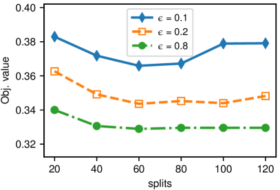
(a) Effect of splits (left: accuracy, right: obj. value)

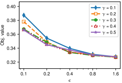
(b) Effect of $\gamma$ (left: accuracy, right: obj. value)

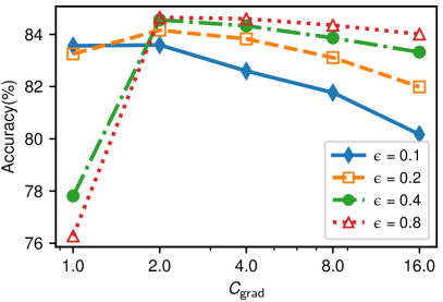
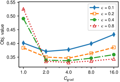
(c) Effect of $C_{\mathsf{grad}}$ (left: accuracy, right: obj. value)

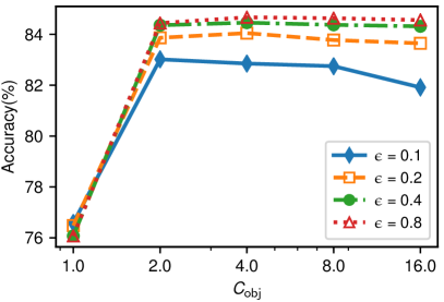
(d) Effect of $C_{\mathsf{obj}}$ (left: accuracy, right: obj. value)

Figure 1. Effects of parameters

In our experiments, to determine the initial privacy budget parameters $\rho_{\mathsf{nmax}}$ and $\rho_{\mathsf{ng}}$, we first compute their corresponding $\epsilon_{\mathsf{namx}}$ and $\epsilon_{\mathsf{ng}}$ values as follows:

$$\epsilon_{\mathsf{nmax}}=\epsilon_{\mathsf{ng}}=\frac{\epsilon_{\mathsf{tot}}}{2\cdot\mathsf{splits}}\,.$$

Then these values are converted back to $\rho_{\mathsf{nmanx}}$ and $\rho_{\mathsf{ng}}$, respectively, using Lemma 3.6 and 3.7. The intuition behind this setting is that the value of splits roughly represents the number of iterations under the naive (linear) composition. We fixed splits=60 for all experiments. Figure 1(a) shows the impacts of splits on the algorithm’s performance. From the figure, we see the performance of DP-AGD is relatively less affected by the choice of splits when $\epsilon$ is large. When $\epsilon=0.1$, excessively small or large value of splits can degrade the performance. When splits is set too small, the algorithm may not have enough number of iterations to converge to the optimum. On the other hand, when the value of splits is too large, the algorithm may find it difficult to discover good search directions.

Figure 1(b) describes how classification accuracy and objective value change with varying values of $\gamma$. The parameter $\gamma$ controls how fast the algorithm increases $\epsilon_{\mathsf{ng}}$ when the gradient for the current iteration is not a descent direction. As it can be seen from the figure, when $\gamma>0.2$, the value of $\gamma$ almost has no impact on the performance. On the other hand, when $\gamma=0.1$ or $\gamma=0.2$, the performance is slightly affected by the setting. This is because, when $\gamma$ is too small, the new estimate of gradient might be still too noisy, and as a result the algorithm spends more privacy budget on executing NoisyMax.

The algorithm has two threshold parameters, $C_{\mathsf{grad}}$ and $C_{\mathsf{obj}}$. These two parameters are used to bound the sensitivity of gradient and objective value computation, respectively. If these parameters are set to a too small value, it significantly reduces the sensitivity but at the same time it can cause too much information loss in the estimates. Conversely, if they are set too high, the sensitivity becomes high, resulting in adding too much noise to the estimates. In our experiments, both $C_{\mathsf{obj}}$ and $C_{\mathsf{grad}}$ are fixed to 3.0.

In Figure 1(c), to see the impact of $C_{\mathsf{grad}}$ on the performance, we fix the objective clipping threshold $C_{\mathsf{obj}}$ to our default value 3.0 and vary $C_{\mathsf{grad}}$ from 1.0 to 16.0. The figure illustrates how the accuracy and the final objective value change with varying values of $C_{\mathsf{grad}}$. We observe that excessively large or small threshold values can degrade the performance. As explained above, this is because of the trade-off between high sensitivity and information loss.

Figure 1(d) shows how $C_{\mathsf{obj}}$ affects the accuracy and the final objective value. As it was the case for $C_{\mathsf{grad}}$, too large or small values have a negative effect on the performance, while the moderate values ($2\leq C_{\mathsf{obj}}\leq 8$) have little impact on the performance.

6.3. Logistic Regression and SVM

We applied our DP-AGD algorithm to a regularized logistic regression model in which the goal is

$$\underset{\bm{\mathrm{w}}}{\min} \frac{1}{n}\sum_{i=1}^{n}\log(1+\exp(-y_{i}\bm{\mathrm{w}}^{\intercal}\bm{\mathrm{x}}_{i}))+\frac{\lambda}{2}\lVert\bm{\mathrm{w}}\rVert_{2}^{2}\,,$$

where $\bm{\mathrm{x}}_{i}\in\mathbb{R}^{p+1}$, $y_{i}\in\{-1,+1\}$, and $\lambda>0$ is a regularization coefficient.

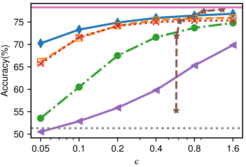
(a) Adult

(b) BANK

(c) IPUMS-US

(d) IPUMS-BR

Figure 2. Logistic regression by varying $\epsilon$ (Top: classification accuracies, Bottom: objective values)

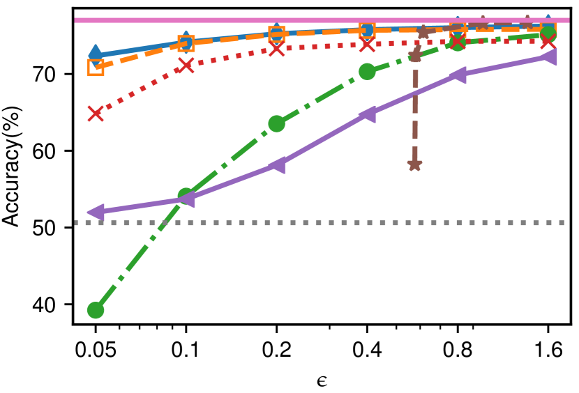
(a) Adult

(b) BANK

(c) IPUMS-US

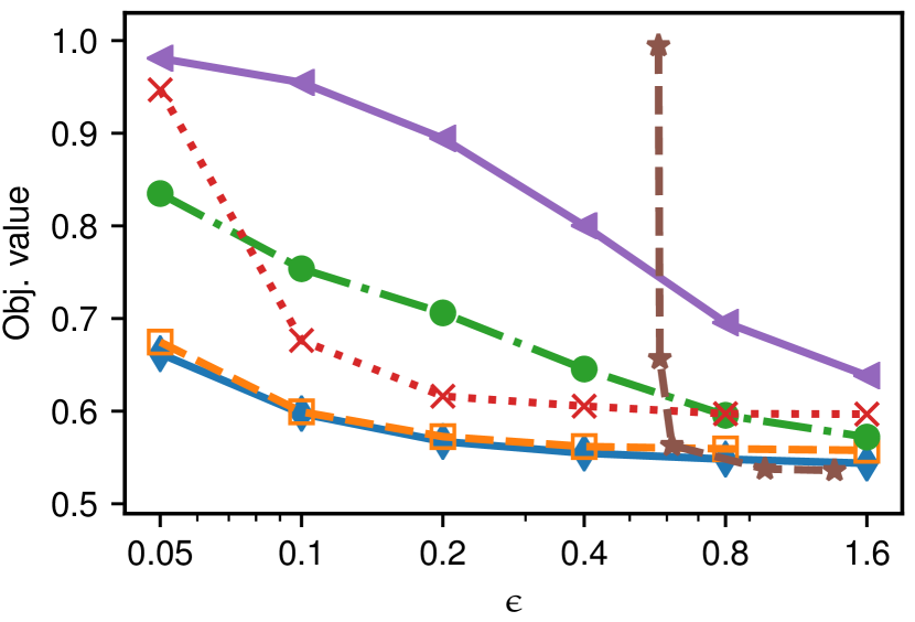
(d) IPUMS-BR

Figure 3. SVM by varying $\epsilon$ (Top: classification accuracies, Bottom: objective values)

Figure 4. Classification task on KDDCup99 dataset (Left: logistic regression, right: SVM)

The top row in Figure 2 shows the classification accuracies of logistic regression model on 4 different datasets. The result on KDDCup99 dataset is shown in Figure 4. The proposed DP-AGD algorithm consistently outperforms or performs competitively with other algorithms on a wide range of $\epsilon$ values. Especially, when $\epsilon$ is very small (e.g., $\epsilon=0.05$), DP-AGD outperforms all other methods except on the BANK dataset. This is because other algorithms tend to waste privacy budgets by obtaining extremely noisy statistics and blindly use them in their updates without checking whether it can lead to a better solution (i.e., they perform many updates that do not help decrease the objective value). On the other hand, DP-AGD explicitly checks the usefulness of the statistics and only use them when they can contribute to decreasing the objective value.

The bottom row of Figure 2 illustrates how the final objective value achieved by each algorithm changes as the value of $\epsilon$ increases. As it was observed in the experiments on classification accuracy, DP-SGD gets close to the best achievable objective values for a wide range of $\epsilon$ values considered in the experiments.

It should be emphasized that the accuracies of SGD-Adv and SGD-MA are largely dependent on the total number of iterations $T$. In all of the baseline algorithms, the value of $T$ needs to be determined before the execution of the algorithms. To get the best accuracy for the given value of $\epsilon$, it requires tuning the value of $T$ through multiple interactions with a dataset (e.g., trial and error), which also should be done in a differentially private manner and hence it requires a portion of privacy budget. In PrivGene, the number of iterations is heuristically set to $T=c\cdot(n\cdot\epsilon)$, where $c$ is a tuning parameter and $n$ is the number of observations in $D$. However, $T$ still requires a careful tuning as it depends on $c$.

SGD-MA outperforms all other algorithms when $\epsilon>0.8$. This is because SGD-MA can afford more number of iterations resulting from tight bound on the privacy loss provided by the moments accountant, together with privacy amplification effect due to subsampling. However, it is hard to use the moments accountant method under high privacy regime (i.e., when $\epsilon$ is small) because the bound is not sharp when there are small number of independent random variables (i.e., when the number of iterations is small). With $\delta$ fixed to $10^{-8}$, we empirically observe that, under the moments accountant, one single iteration of SGD update can incur the privacy cost of $\epsilon\approx 0.5756$. This renders the moments accountant method impractical when high level of privacy protection is required.

Support vector machine (SVM) is one of the most effective tools for classification problems. In this work, we only consider the linear SVM (without kernel) for simplicity. The SVM classification problem is formulated as an optimization problem:

$$\underset{\bm{\mathrm{w}}}{\min} \frac{\lambda}{2}\lVert\bm{\mathrm{w}}\rVert_{2}^{2}+\frac{1}{n}\sum_{i=1}^{n}\max\{1-y_{i}\bm{\mathrm{w}}^{\intercal}\bm{\mathrm{x}}_{i},0\}\,,$$

where $\bm{\mathrm{x}}_{i}\in\mathbb{R}^{p+1}$ and $y_{i}\in\{-1,+1\}$ for $i\in[n]$.

Figure 3 compares the performance of DP-AGD on SVM task with other baseline algorithms. As it was shown in the experiments on logistic regression, DP-AGD achieves the competitive accuracies on a wide range of values for $\epsilon$.

DP-AGD showed an unstable behavior when performing SVM task on BANK dataset: its accuracy can degrade even though we use more privacy budget. For example, the accuracy when $\epsilon=0.4$ is lower than that when $\epsilon=0.1$. However, we observe that its objective value consistently decreases as the value of $\epsilon$ is increased.

7. Conclusion

This paper has developed an iterative optimization algorithm for differential privacy, in which the per-iteration privacy budget is adaptively determined based on the utility of privacy-preserving statistics. Existing private algorithms lack runtime adaptivity to account for statistical utility of intermediate query answers. To address this significant drawback, we presented a general framework for adaptive privacy budget selection. While the proposed algorithm has been demonstrated in the context of private ERM problem, we believe our approach can be easily applied to other problems.

References

- (1)
- Abadi et al. (2016) Martin Abadi, Andy Chu, Ian Goodfellow, H Brendan McMahan, Ilya Mironov, Kunal Talwar, and Li Zhang. 2016. Deep learning with differential privacy. In Proceedings of the 2016 ACM SIGSAC Conference on Computer and Communications Security. ACM, 308–318.
- Bassily et al. (2014) Raef Bassily, Adam Smith, and Abhradeep Thakurta. 2014. Private Empirical Risk Minimization: Efficient Algorithms and Tight Error Bounds. In Proceedings of the 2014 IEEE 55th Annual Symposium on Foundations of Computer Science (FOCS ’14). IEEE Computer Society, Washington, DC, USA, 464–473.
- Beimel et al. (2014) Amos Beimel, Hai Brenner, Shiva Prasad Kasiviswanathan, and Kobbi Nissim. 2014. Bounds on the sample complexity for private learning and private data release. Machine learning 94, 3 (2014), 401–437.
- Bun and Steinke (2016) Mark Bun and Thomas Steinke. 2016. Concentrated differential privacy: Simplifications, extensions, and lower bounds. In Theory of Cryptography Conference. Springer, 635–658.
- Chang and Lin (2011) Chih-Chung Chang and Chih-Jen Lin. 2011. LIBSVM: a library for support vector machines. ACM transactions on intelligent systems and technology (TIST) 2, 3 (2011), 27.
- Chaudhuri et al. (2011) Kamalika Chaudhuri, Claire Monteleoni, and Anand D Sarwate. 2011. Differentially private empirical risk minimization. Journal of Machine Learning Research 12, Mar (2011), 1069–1109.
- Dwork et al. (2006a) Cynthia Dwork, Krishnaram Kenthapadi, Frank McSherry, Ilya Mironov, and Moni Naor. 2006a. Our data, ourselves: Privacy via distributed noise generation. In Annual International Conference on the Theory and Applications of Cryptographic Techniques. Springer, 486–503.
- Dwork et al. (2006b) Cynthia Dwork, Frank McSherry, Kobbi Nissim, and Adam Smith. 2006b. Calibrating noise to sensitivity in private data analysis. In Theory of Cryptography Conference. Springer, 265–284.
- Dwork et al. (2014) Cynthia Dwork, Aaron Roth, et al. 2014. The algorithmic foundations of differential privacy. Foundations and Trends® in Theoretical Computer Science 9, 3–4 (2014), 211–407.
- Dwork et al. (2010) C. Dwork, G. N. Rothblum, and S. Vadhan. 2010. Boosting and Differential Privacy. In 2010 IEEE 51st Annual Symposium on Foundations of Computer Science. 51–60.
- Jain et al. (2012) Prateek Jain, Pravesh Kothari, and Abhradeep Thakurta. 2012. Differentially private online learning. In Conference on Learning Theory. 24–1.
- Kifer et al. (2012) Daniel Kifer, Adam Smith, and Abhradeep Thakurta. 2012. Private convex empirical risk minimization and high-dimensional regression. In Conference on Learning Theory. 25–1.
- Lichman (2013) M. Lichman. 2013. UCI Machine Learning Repository. (2013). http://archive.ics.uci.edu/ml
- Nocedal (1980) Jorge Nocedal. 1980. Updating quasi-Newton matrices with limited storage. Mathematics of computation 35, 151 (1980), 773–782.
- Nocedal and Wright (2006) J. Nocedal and S. J. Wright. 2006. Numerical Optimization (2nd ed.). Springer, New York.
- Robbins and Monro (1951) Herbert Robbins and Sutton Monro. 1951. A stochastic approximation method. The annals of mathematical statistics (1951), 400–407.
- Rubinstein et al. (2012) Benjamin IP Rubinstein, Peter L Bartlett, Ling Huang, and Nina Taft. 2012. Learning in a Large Function Space: Privacy-Preserving Mechanisms for SVM Learning. Journal of Privacy and Confidentiality 4, 1 (2012), 4.
- Ruggles et al. ([n. d.]) Steven Ruggles, Katie Genadek, Ronald Goeken, Josiah Grover, and Matthew Sobek. [n. d.]. Integrated Public Use Microdata Series, Minnesota Population Center. http://international.ipums.org. ([n. d.]).
- Song et al. (2013) S. Song, K. Chaudhuri, and A. D. Sarwate. 2013. Stochastic gradient descent with differentially private updates. In GlobalSIP.
- Talwar et al. (2015) Kunal Talwar, Abhradeep Guha Thakurta, and Li Zhang. 2015. Nearly optimal private lasso. In Advances in Neural Information Processing Systems. 3025–3033.
- Wang et al. (2017) Di Wang, Minwei Ye, and Jinhui Xu. 2017. Differentially Private Empirical Risk Minimization Revisited: Faster and More General. In Advances in Neural Information Processing Systems 30. Curran Associates, Inc., 2719–2728.
- Wang et al. (2015) Yu-Xiang Wang, Stephen Fienberg, and Alex Smola. 2015. Privacy for free: Posterior sampling and stochastic gradient monte carlo. In International Conference on Machine Learning. 2493–2502.
- Williams and McSherry (2010) Oliver Williams and Frank McSherry. 2010. Probabilistic inference and differential privacy. In Proceedings of the 23rd International Conference on Neural Information Processing Systems-Volume 2. Curran Associates Inc., 2451–2459.
- Zhang et al. (2013) Jun Zhang, Xiaokui Xiao, Yin Yang, Zhenjie Zhang, and Marianne Winslett. 2013. PrivGene: Differentially Private Model Fitting Using Genetic Algorithms. In Proceedings of the 2013 ACM SIGMOD International Conference on Management of Data (SIGMOD ’13). ACM, New York, NY, USA, 665–676.
- Zhang et al. (2017) Jiaqi Zhang, Kai Zheng, Wenlong Mou, and Liwei Wang. 2017. Efficient private ERM for smooth objectives. In Proceedings of the 26th International Joint Conference on Artificial Intelligence. AAAI Press, 3922–3928.