Appeared in the proceedings of EMNLP 2018 (Brussels, October). This version was
prepared in October 2018 and fixes some minor mistakes .
A Discriminative Latent-Variable Model for Bilingual Lexicon Induction

Abstract

We introduce a novel discriminative latent-variable model for the task of bilingual lexicon induction. Our model combines the bipartite matching dictionary prior of Haghighi et al. (2008) with a state-of-the-art embedding-based approach. To train the model, we derive an efficient Viterbi EM algorithm. We provide empirical improvements on six language pairs under two metrics and show that the prior theoretically and empirically helps to mitigate the hubness problem. We also demonstrate how previous work may be viewed as a similarly fashioned latent-variable model, albeit with a different prior.

1 Introduction

Is there a more fundamental bilingual linguistic resource than a dictionary? The task of bilingual lexicon induction seeks to create a dictionary in a data-driven manner directly from monolingual corpora in the respective languages and, perhaps, a small seed set of translations. From a practical point of view, bilingual dictionaries have found uses in a myriad of NLP tasks ranging from machine translation Klementiev et al. (2012) to cross-lingual named entity recognition Mayhew et al. (2017). In this work, we offer a probabilistic twist on the task, developing a novel discriminative latent-variable model that outperforms previous work.

Our proposed model is a bridge between current state-of-the-art methods in bilingual lexicon induction that take advantage of word embeddings, e.g., the embeddings induced by Mikolov et al. (2013b)'s skip-gram objective, and older ideas in the literature that build explicit probabilistic models for the task. We propose a discriminative probability model, inspired by Irvine and Callison-Burch (2013), infused with the bipartite matching dictionary prior of Haghighi et al. (2008). However, like more recent approaches Artetxe et al. (2017), our model operates directly over pretrained word embeddings, induces a joint cross-lingual embedding space, and scales to large vocabulary sizes. To train our model, we derive a generalized expectation-maximization algorithm (EM; Neal and Hinton, 1998) and employ an efficient matching algorithm.

Empirically, we experiment on three standard and three extremely low-resource language pairs. We evaluate intrinsically, comparing the quality of the induced bilingual dictionary, as well as analyzing the resulting bilingual word embeddings themselves. The latent-variable model yields gains over several previous approaches across language pairs. It also enables us to make implicit modeling assumptions explicit. To this end, we provide a reinterpretation of Artetxe et al. (2017) as a latent-variable model with an IBM Model 1–style Brown et al. (1993) dictionary prior, which allows a clean side-by-side analytical comparison. Viewed in this light, the difference between our approach and Artetxe et al. (2017), the strongest baseline, is whether one-to-one alignments or one-to-many alignments are admitted between the words of the languages' respective lexicons. Thus, we conclude that our hard constraint on one-to-one alignments is primarily responsible for the improvements over Artetxe et al. (2017).

2 Background: Bilingual Lexicon Induction and Word Embeddings

Bilingual lexicon induction is the task of finding word-level translations between the lexicons of two languages. For instance, the German word Hund and the English word dog are roughly semantically equivalent, so the pair Hund–dog should be an entry in a German–English bilingual lexicon. The task itself comes in a variety of flavors. We consider a version of the task that only relies on monolingual corpora in the tradition of Rapp (1995) and Fung (1995). In other words, the goal is to produce a bilingual lexicon primarily from unannotated raw text in each of the respective languages. Importantly, we avoid reliance on bitext, i.e. corpora with parallel sentences that are known translations of each other, e.g., EuroParl Koehn (2005). The bitext assumption is quite common in the literature; see Ruder et al. (2018, Table 2) for a survey. Additionally, we will assume the existence of a small seed set of word-level translations obtained from a dictionary; we also experiment with seed sets obtained from heuristics that do not rely on the existence of linguistic resources.

2.1 Graph-Theoretic Formulation

To ease the later exposition, we will formulate the task graph-theoretically. Let $\ell_{\textit{src}}$ denote the source language and $\ell_{\textit{trg}}$ the target language. Suppose the source language $\ell_{\textit{src}}$ has $n_{\textit{src}}$ word types in its lexicon $V_{\textit{src}}$ and $\ell_{\textit{trg}}$ has $n_{\textit{trg}}$ word types in its lexicon $V_{\textit{trg}}$. We will write $v_{\textit{src}}(i)$ for the $i^{\text{th}}$ word type in $\ell_{\textit{src}}$ and $v_{\textit{trg}}(i)$ for the $i^{\text{th}}$ word type in $\ell_{\textit{trg}}$. We can view the elements of $V_{\textit{src}}$ and $V_{\textit{trg}}$ as sets of vertices in a graph. Now consider the bipartite set of vertices $V=V_{\textit{trg}}\cup V_{\textit{src}}$. In these terms, a bilingual lexicon is just a bipartite graph $G=(E,V)$ and, thus, the task of bilingual lexicon induction is a combinatorial problem: the search for a `good' edge set $E\subseteq V_{\textit{trg}}\times V_{\textit{src}}$. We depict such a bipartite graph in Figure 1. In § 3, we will operationalize the notion of `goodness' by assigning a weight $w_{ij}$ to each possible edge between $V_{\textit{trg}}$ and $V_{\textit{src}}$.

When the edge set $E$ takes the form of a matching, we will denote it as $\mathbf{m}$. In general, we will be interested in partial matchings, where many vertices have no incident edges. We will write ${\cal M}$ for the set of all partial matchings on the bipartite graph $G$. The set of vertices in $V_{\textit{trg}}$ (respectively $V_{\textit{src}}$) with no incident edges will be termed $\mathbf{u}_{\textit{trg}}$ (respectively $\mathbf{u}_{\textit{src}}$). Note that for any matching $\mathbf{m}$, we have the identity $\mathbf{u}_{\textit{trg}}=V_{\textit{trg}}\setminus\{i:(i,j)\in\mathbf{m}\}$.

Figure 1: Partial lexicons of German and English shown as a bipartite graph. German is the target language and English is the source language. The $n_{\textit{trg}}=7$ German words are shown in blue and the $n_{\textit{src}}=6$ English words are shown in green. A bipartite matching $\mathbf{m}$ between the two sets of vertices is also depicted. The German nodes in $\mathbf{u}_{\textit{trg}}$ are unmatched.

2.2 Word Embeddings

Word embeddings will also play a key role in our model. For the remainder of the paper, we will assume we have access to $d$-dimensional embeddings for each language's lexicon—for example, those provided by a standard model such as skip-gram Mikolov et al. (2013b). Notationally, we define the real matrices $S\in\mathbb{R}^{d\times n_{\textit{src}}}$ and $T\in\mathbb{R}^{d\times n_{\textit{trg}}}$. Note that in this formulation $s_{i}\in\mathbb{R}^{d}$, the $i^{\text{th}}$ column of $S$, is the word embedding corresponding to $v_{\textit{src}}(i)$. Likewise, note that $t_{i}\in\mathbb{R}^{d}$, the $i^{\text{th}}$ column of $T$, is the word embedding corresponding to $v_{\textit{trg}}(i)$.

3 A Latent-Variable Model

The primary contribution of this paper is a novel latent-variable model for bilingual lexicon induction. The latent variable will be the edge set $E$, as discussed in § 2.1. Given pretrained embeddings for the source and target languages, arranged into the matrices $S$ and $T$, we define the density

$$p(T\mid S)\coloneqq\sum_{\mathbf{m}\in{\cal M}}p(T\mid S,\mathbf{m})\cdot p(\mathbf{m})$$ (1)

where, recall from § 2, ${\cal M}$ is the set of all bipartite matchings on the graph $G$ and $\mathbf{m}\in{\cal M}$ is an individual matching. Note that, then, $p(\mathbf{m})$ is a distribution over all bipartite matchings on $G$ such as the matching shown in Figure 1. We will take $p(\mathbf{m})$ to be fixed as the uniform distribution for the remainder of the exposition, though more complicated distributions could be learned, of course. We further define the distribution

$$p_{\theta}(T\mid S,\mathbf{m})\coloneqq\prod_{(i,j)\in\mathbf{m}}p(t_{i}\mid s_{j})\cdot\prod_{i\in\mathbf{u}_{\textit{trg}}}p(t_{i})$$ (2)

Recall we write $(i,j)\in\mathbf{m}$ to denote an edge in the matching. Furthermore, for notational simplicity, we have dropped the dependence of $\mathbf{u}_{\textit{trg}}$ on $\mathbf{m}$. (Recall $\mathbf{u}_{\textit{trg}}=V_{\textit{trg}}\setminus\{i:(i,j)\in\mathbf{m}\}$). Next, we define the two densities present in equation 2 as Gaussians:

$$p_{\theta}(t\mid s) \coloneqq{\cal N}\left(\Omega\,s,I\right)$$ (3)

$$\propto\exp-\nicefrac{{1}}{{2}}||t-\Omega\,s||_{2}^{2}$$

$$p_{\theta}(t) \coloneqq{\cal N}\left(\mu,I\right)$$ (4)

Given a fixed matching $\mathbf{m}$, we may create matrices $S_{\mathbf{m}}\in\mathbb{R}^{d\times|\mathbf{m}|}$ and $T_{\mathbf{m}}\in\mathbb{R}^{d\times|\mathbf{m}|}$ such that the rows correspond to word vectors of matched vertices (translations under the matching $\mathbf{m}$). Now, after some algebra, we see that we can rewrite $\prod_{(i,j)\in\mathbf{m}}p(t_{i}\mid s_{i})$ in matrix notation:

$$p_{\theta}(T_{\mathbf{m}}\mid S_{\mathbf{m}},\mathbf{m}) =\prod_{(i,j)\in\mathbf{m}}p(t_{i}\mid s_{j})$$ (5)

$$\propto\prod_{(i,j)\in\mathbf{m}}\exp-\nicefrac{{1}}{{2}}||t_{i}-\Omega\,s_{j}||_{2}^{2}$$

$$=\exp\sum_{(i,j)\in\mathbf{m}}-\nicefrac{{1}}{{2}}||t_{i}-\Omega\,s_{j}||_{2}^{2}$$

$$=\exp-\nicefrac{{1}}{{2}}||T_{\mathbf{m}}-\Omega\,S_{\mathbf{m}}||_{F}^{2}$$ (6)

where $\Omega\in\mathbb{R}^{d\times d}$ is an orthogonal matrix of parameters to be learned. The result of this derivation, equation 6, will become useful during the discussion of parameter estimation in § 4.

We define the model's parameters, to be optimized, as $\theta=\left(\Omega,\mu\right)$.

Modeling Assumptions and their Limitations

In the previous section, we have formulated the induction of a bilingual lexicon as the search for an edge set $E$, which we treat as a latent variable that we marginalize out in equation 2. Specifically, we assume that $E$ is a partial matching. Thus, for every $(i,j)\in\mathbf{m}$, we have $t_{i}\sim\mathcal{N}\left(\Omega\,s_{j},I\right)$, that is, the embedding for $v_{\textit{trg}}(i)$ is assumed to have been drawn from a Gaussian centered around the embedding for $v_{\textit{src}}(j)$, after an orthogonal transformation. This gives rise to two modeling assumptions, which we make explicit: (i) There exists a single source for every word in the target lexicon and that source cannot be used more than once. (ii) There exists an orthogonal transformation, after which the embedding spaces are more or less equivalent.

Assumption (i) may be true for related languages, but is likely false for morphologically rich languages that have a many-to-many relationship between the words in their respective lexicons. We propose to ameliorate this using a rank constraint that only considers the top $n$ most frequent words in both lexicons for matching in § 6. In addition, we experiment with priors that express different matchings in § 7.

As for assumption (ii), previous work Xing et al. (2015); Artetxe et al. (2017) has achieved some success using an orthogonal transformation; recently, however, Søgaard et al. (2018) demonstrated that monolingual embedding spaces are not approximately isomorphic and that there is a complex relationship between word form and meaning, which is only inadequately modeled by current approaches, which for example cannot model polysemy. Nevertheless, we will show that imbuing our model with these assumptions helps empirically in § 6, giving them practical utility.

Why it Works: The Hubness Problem

Why should we expect the bipartite matching prior to help, given that we know of cases when multiple source words should match a target word? One answer is because the bipartite prior helps us obviate the hubness problem, a common issue in word-embedding-based bilingual lexicon induction Dinu et al. (2015). The hubness problem is an intrinsic problem of high-dimensional vector spaces where certain vectors will be universal nearest neighbors, i.e. they will be the nearest neighbor to a disproportionate number of other vectors Radovanović et al. (2010). Thus, if we allow one-to-many alignments, we will find the embeddings of certain elements of $V_{\textit{src}}$ acting as hubs, i.e. the model will pick them to generate a disproportionate number of target embeddings, which reduces the quality of the embedding space.

Another explanation for the positive effect of the one-to-one alignment prior is its connection to the Wasserstein distance and computational optimal transport Villani (2008). Concurrent work Grave et al. (2018) similarly has found the one-to-one alignment prior to be beneficial.

4 Parameter Estimation

We will conduct parameter estimation through Viterbi EM. We describe first the E-step, then the M-step. Viterbi EM estimates the parameters by alternating between the two steps until convergence. We give the complete pseudocode in Algorithm 1.

1:repeat

2:     // Viterbi E-Step

3:     $\mathbf{m}^{\star}\leftarrow\text{argmax}_{\mathbf{m}\in{\cal M}}\log p_{\theta}(\mathbf{m}\mid S,T)$

4:     $\mathbf{u}_{\textit{trg}}^{\star}\leftarrow V_{\textit{trg}}\setminus\{i:(i,j)\in\mathbf{m}^{\star}\}$ author=Ryan,color=violet!40,size=,fancyline,caption=,inline,]Sebastian, can you check that I took the SVD of the right matrix? author=Sebastian,color=green!40,size=,fancyline,caption=,inline,]Just checked. I think it's $T^{\top}S$ instead of $ST^{\top}$. That's also what we use in the vecmap code.

5:     // M-Step

6:     $U\Sigma V^{\top}\leftarrow\texttt{SVD}\left(T_{\mathbf{m}^{\star}}S^{\top}_{\mathbf{m}^{\star}}\right)$

7:     $\Omega^{\star}\leftarrow UV^{\top}$

8:     $\mu^{\star}\leftarrow\nicefrac{{1}}{{|\mathbf{u}_{\textit{trg}}^{\star}|}}\cdot\sum_{i\in\mathbf{u}_{\textit{trg}}^{\star}}t_{i}$

9:     $\mathbf{\theta}\leftarrow\left(\Omega^{\star},\mu^{\star}\right)$

10:until converged

Algorithm 1 Viterbi EM for our latent-variable model

4.1 Viterbi E-Step

The E-step asks us to compute the posterior of latent bipartite matchings $p(\mathbf{m}\mid S,T)$. Computation of this distribution, however, is intractable as it would require a sum over all bipartite matchings, which is #P-hard Valiant (1979). Tricks from combinatorial optimization make it possible to maximize over all bipartite matchings in polynomial time. Thus, we fall back on the Viterbi approximation for the E-step Brown et al. (1993); Samdani et al. (2012). The derivation will follow Haghighi et al. (2008). In order to compute author=Ryan,color=violet!40,size=,fancyline,caption=,inline,]We really need to clean this up for the camera ready…the construction in Haghighi et al. (2008) is mathematically sound, whereas what we are doing is not. We need to reformulate it as as a pruned partial bipartite matching problem.

$$\mathbf{m}^{\star}=\underset{\mathbf{m}\in{\cal M}}{\text{argmax}}\log p_{\theta}(\mathbf{m}\mid S,T)$$ (7)

we construct a fully connected bipartite graph $G=(E,V_{\textit{src}}\cup V_{\textit{trg}})$, where $E=V_{\textit{src}}\times V_{\textit{trg}}$. We weight each arc $(i,j)\in E$ with the weight between the projected source word and target word embeddings: $w_{ij}=\log p(t_{i}\mid s_{j})-\log p(t_{i})=\nicefrac{{-1}}{{2}}\left(||t_{i}-\Omega\,s_{j}||_{2}^{2}-||t_{i}-\mu||_{2}^{2}\right)$, where the normalizers of both Gaussians cancel as both have the same covariance matrix, i.e., $I$. Note that in the case where the $t_{i}$ and the $s_{j}$ are of length 1, that is, $||t_{i}||_{2}=||s_{j}||_{2}=1$, and $\mu=\mathbf{0}$, we recover cosine similarity between the vectors up to an additive constant as orthogonal matrices preserve length (the constant is always $-\nicefrac{{1}}{{2}}$ as $||t_{i}||_{2}=1$). We may ignore this constant during the E-step's combinatorial optimization. Note the optimal partial matching will contain no edges with weight $w_{ij}<0$. For this reason, we remove such edges from the bipartite graph. author=Ryan,color=violet!40,size=,fancyline,caption=,inline,]This is no longer really EM. We need to adjust the lack of the prior in this expression. To find the maximal partial bipartite matching on $G$ to compute $\mathbf{m}^{\star}$, we employ an efficient algorithm as detailed in the next section.

Finding a Maximal Bipartite Matching

We frame finding an optimal one-to-one alignment between $n_{\textit{src}}$ source and $n_{\textit{trg}}$ words as a combinatorial optimization problem, specifically, a linear assignment problem (LAP; Bertsimas and Tsitsiklis, 1997). In its original formulation, the LAP requires assigning a number of agents (source words) to a number of tasks (target words) at a cost that varies based on each assignment. An optimal solution assigns each source word to exactly one target word and vice versa at minimum cost. The Hungarian algorithm Kuhn (1955) is one of the most well-known approaches for solving the LAP, but runs in $O((n_{src}+n_{trg})^{3})$. This works for smaller vocabulary sizes, but is prohibitive for matching cross-lingual word embeddings with large vocabularies for real-world applications.

For each source word, most target words, however, are unlikely candidates for alignment. We thus propose to consider only the top $k$ most similar target words for alignment with every source word. We sparsify the graph by weighting the edges for all other words with $-\infty$. The remaining weights $w_{ij}$ are chosen as discussed above. We employ a version of the Jonker-Volgenant algorithm Jonker and Volgenant (1987); Volgenant (1996), which has been optimized for LAP on sparse graphs, to find the maximum-weight matching $\mathbf{m}^{\star}$ on $G$.

4.2 M-Step

Next, we will describe the M-step. Given an optimal matching $\mathbf{m}^{\star}$ computed in § 4.1, we search for a matrix $\Omega\in\mathbb{R}^{d\times d}$. We additionally enforce the constraint that $\Omega$ is a real orthogonal matrix, i.e., $\Omega^{\top}\Omega=I$. Previous work Xing et al. (2015); Artetxe et al. (2017) found that the orthogonality constraint leads to noticeable improvements.

Our M-step optimizes two objectives independently. First, making use of the result in equation 6, we optimize the following:

$$-\log p(T_{\mathbf{m}^{\star}}\mid S_{\mathbf{m}^{\star}}, \mathbf{m}^{\star})$$ (8)

$$=||T_{\mathbf{m}^{\star}}-\Omega\,S_{\mathbf{m}^{\star}}||_{F}^{2}+C$$

with respect to $\Omega$ subject to $\Omega^{\top}\Omega=I$. (Note we may ignore the constant $C$ during the optimization.) Second, we optimize the objective

$$-\log\prod_{i\in\mathbf{u}_{\textit{trg}}}p(t_{i})=\sum_{i\in\mathbf{u}_{\textit{trg}}}||t_{i}-\mu||_{2}^{2}+D$$ (9)

with respect to the mean parameter $\mu$, which is simply an average. Note, again, we may ignore the constant $D$ during optimization.

Optimizing equation 8 with respect to $\Omega$ is known as the orthogonal Procrustes problem Schönemann (1966); Gower and Dijksterhuis (2004) and has a closed form solution that exploits the singular value decomposition Horn and Johnson (2012). Namely, we compute $U\Sigma V^{\top}=T_{\mathbf{m}}^{\top}S_{\mathbf{m}}$. Then, we directly arrive at the optimum: $\Omega^{\star}=UV^{\top}$. Optimizing equation 9 can also been done in closed form; the point which minimizes distance to the data points (thereby maximizing the log-probability) is the centroid: $\mu^{\star}=\nicefrac{{1}}{{|\mathbf{u}_{\textit{trg}}|}}\cdot\sum_{i\in\mathbf{u}_{\textit{trg}}}t_{i}$.

5 Reinterpretation of Artetxe et al. (2017) as a Latent-Variable Model

The self-training method of Artetxe et al. (2017), our strongest baseline in § 6, may also be interpreted as a latent-variable model in the spirit of our exposition in § 3. Indeed, we only need to change the edge-set prior $p(\mathbf{m})$ to allow for edge sets other than those that are matchings. Specifically, a matching enforces a one-to-one alignment between types in the respective lexicons. Artetxe et al. (2017), on the other hand, allow for one-to-many alignments. We show how this corresponds to an alignment distribution that is equivalent to IBM Model 1 Brown et al. (1993), and that Artetxe et al. (2017)'s self-training method is actually a form of Viterbi EM.

To formalize Artetxe et al. (2017)'s contribution as a latent-variable model, we lay down some more notation. Let ${\cal A}=\{1,\ldots,n_{\textit{src}}+1\}^{n_{\textit{trg}}}$, where we define $(n_{\textit{src}}+1)$ to be none, a distinguished symbol indicating unalignment. The set ${\cal A}$ is to be interpreted as the set of all one-to-many alignments $\mathbf{a}$ on the bipartite vertex set $V=V_{\textit{trg}}\cup V_{\textit{src}}$ such that $a_{i}=j$ means the $i^{\text{th}}$ vertex in $V_{\textit{trg}}$ is aligned to the $j^{\text{th}}$ vertex in $V_{\textit{src}}$. Note that $a_{i}=(n_{\textit{src}}+1)=\texttt{none}$ means that the $i^{\text{th}}$ element of $V_{\textit{trg}}$ is unaligned. Now, by analogy to our formulation in § 3, we define

$$p(T\mid S) \coloneqq\sum_{\mathbf{a}\in{\cal A}}p(T\mid S,\mathbf{a})\cdot p(\mathbf{a})$$ (10)

$$=\sum_{\mathbf{a}\in{\cal A}}\prod_{i=1}^{n_{\textit{trg}}}p(t_{i}\mid s_{a_{i}},a_{i})\cdot p(a_{i})$$ (11)

$$=\prod_{i=1}^{n_{\textit{trg}}}\sum_{{a_{i}}=1}^{n_{\textit{src}}+1}p(t_{i}\mid s_{a_{i}},a_{i})\cdot p(a_{i})$$ (12)

The move from equation 11 to equation 12 is the dynamic-programming trick introduced in Brown et al. (1993). This reduces the number of terms in the expression from exponentially many to polynomially many. We take $p(\mathbf{a})$ to be a uniform distribution over all alignments with no parameters to be learned.

Artetxe et al. (2017)'s Viterbi E-Step

In the context of Viterbi EM, it means the max over ${\cal A}$ will decompose additively s

$$\underset{\mathbf{a}\in{\cal A}}{\max}\log p(\mathbf{a}\mid S,T)=\sum_{i=1}^{n_{\textit{trg}}}\!\!\!\!\!\!\!\!\!\!\!\underset{\hskip 21.33955pt1\leq a_{i}\leq(n_{\textit{src}}+1)}{\max}\!\!\!\!\!\!\!\!\!\!\!\!\!\!\!\log p(a_{i}\mid S,T)$$

thus, we can simply find $\mathbf{a}^{\star}$ component-wise as follows:

$$a_{i}^{\star}=\!\!\!\!\!\!\underset{1\leq a_{i}\leq(n_{\textit{src}}+1)}{\text{argmax}}\!\!\!\!\!\log p(a_{i}\mid t_{i},s_{a_{i}})$$ (13)

Artetxe et al. (2017)'s M-step

The M-step remains unchanged from the exposition in § 3 with the exception that we fit $\Omega$ given matrices $S_{\mathbf{a}}$ and $T_{\mathbf{a}}$ formed from a one-to-many alignment $\mathbf{a}$, rather than a matching $\mathbf{m}$.

Why a Reinterpretation?

The reinterpretation of Artetxe et al. (2017) as a probabilistic model yields a clear analytical comparison between our method and theirs. The only difference between the two is the constraint on the bilingual lexicon that the model is allowed to induce. author=Ryan,color=violet!40,size=,fancyline,caption=,inline,]Say more here? The point is that we have an ablation study.

English–Italian English–German English–Finnish 5,000 25 num iden 5,000 25 num iden 5,000 25 num iden Mikolov et al. (2013c) 34.93 00.00 0.00 1.87 35.00 0.00 0.07 19.20 25.91 0.00 0.00 7.02 Xing et al. (2015) 36.87 0.00 0.13 27.13 41.27 0.07 0.53 38.13 28.23 0.07 0.56 17.95 Zhang et al. (2016) 36.73 0.07 0.27 28.07 40.80 0.13 0.87 38.27 28.16 0.14 0.42 17.56 Artetxe et al. (2016) 39.27 0.07 0.40 31.07 41.87 0.13 0.73 41.53 30.62 0.21 0.77 22.61 Artetxe et al. (2017) 39.67 37.27 39.40 39.97 40.87 39.60 40.27 40.67 28.72 28.16 26.47 27.88 Ours (1:1) 41.00 39.63 40.47 41.07 42.60 42.40 42.60 43.20 29.78 0.07 3.02 29.76 Ours (1:1, rank constr.) 42.47 41.13 41.40 41.80 41.93 42.40 41.93 41.47 28.23 27.04 27.60 27.81

Table 1: Precision at 1 (P@1) scores for bilingual lexicon induction of different models with different seed dictionaries and languages on the full vocabulary.

en-it en-de Dict WS RG WS Mikolov et al. (2013c) 5k .627 .643 .528 Xing et al. (2015) 5k .614 .700 .595 Zhang et al. (2016) 5k .616 .704 .596 Artetxe et al. (2016) 5k .617 .716 .597 Artetxe et al. (2017) 5k .624 .742 .616 25 .626 .749 .612 num .628 .739 .604 Ours (1:1) 5k .621 .733 .618 25 .621 .740 .617 num .624 .743 .617 Ours (1:1, rank constr.) 5k .623 .741 .609 25 .622 .753 .609 num .625 .755 .611

Table 2: Spearman correlations on English–Italian and English–German cross-lingual word similarity datasets.

6 Experiments

We first conduct experiments on bilingual dictionary induction and cross-lingual word similarity on three standard language pairs, English–Italian, English–German, and English–Finnish.

6.1 Experimental Details

Datasets

For bilingual dictionary induction, we use the English–Italian dataset by Dinu et al. (2015) and the English–German and English–Finnish datasets by Artetxe et al. (2017). For cross-lingual word similarity, we use the RG-65 and WordSim-353 cross-lingual datasets for English–German and the WordSim-353 cross-lingual dataset for English–Italian by Camacho-Collados et al. (2015).

Monolingual Embeddings

We follow Artetxe et al. (2017) and train monolingual embeddings with word2vec, CBOW, and negative sampling Mikolov et al. (2013a) on a 2.8 billion word corpus for English (ukWaC + Wikipedia + BNC), a 1.6 billion word corpus for Italian (itWaC), a 0.9 billion word corpus for German (SdeWaC), and a 2.8 billion word corpus for Finnish (Common Crawl).

Seed dictionaries

Following Artetxe et al. (2017), we use dictionaries of 5,000 words, 25 words, and a numeral dictionary consisting of words matching the [0-9]+ regular expression in both vocabularies. In line with Søgaard et al. (2018), we additionally use a dictionary of identically spelled strings in both vocabularies.

Implementation details

Similar to Artetxe et al. (2017), we stop training when the improvement on the average cosine similarity for the induced dictionary is below $1\times 10^{-6}$ between succeeding iterations. Unless stated otherwise, we induce a dictionary of 200,000 source and 200,000 target words as in previous work Mikolov et al. (2013c); Artetxe et al. (2016). For optimal 1:1 alignment, we have observed the best results by keeping the top $k=3$ most similar target words. If using a rank constraint, we restrict the matching in the E-step to the top 40,000 words in both languages. Finding an optimal alignment on the 200,000 $\times$ 200,000 graph takes about 25 minutes on CPU; with a rank constraint, matching takes around three minutes.

Baselines

We compare our approach with and without the rank constraint to the original bilingual mapping approach by Mikolov et al. (2013c). In addition, we compare with Zhang et al. (2016) and Xing et al. (2015) who augment the former with an orthogonality constraint and normalization and an orthogonality constraint respectively. Finally, we compare with Artetxe et al. (2016) who add dimension-wise mean centering to Xing et al. (2015), and Artetxe et al. (2017).

Both Mikolov et al. (2013c) and Artetxe et al. (2017) are special cases of our famework and comparisons to these approaches thus act as an ablation study. Specifically, Mikolov et al. (2013c) does not employ orthogonal Procrustes, but rather allows the learned matrix $\Omega$ to range freely. Likewise, as discussed in § 5, Artetxe et al. (2017) make use of a Viterbi EM style algorithm with a different prior over edge sets.

6.2 Results

We show results for bilingual dictionary induction in Table 1 and for cross-lingual word similarity in Table 2. Our method with a 1:1 prior outperforms all baselines on English–German and English–Italian. Interestingly, the 1:1 prior by itself fails on English–Finnish with a 25 word and numerals seed lexicon. We hypothesize that the prior imposes too strong of a constraint to find a good solution for a distant language pair from a poor initialization. With a better—but still weakly supervised—starting point using identical strings, our approach finds a good solution. Alternatively, we can mitigate this deficiency effectively using a rank constraint, which allows our model to converge to good solutions even with a 25 word or numerals seed lexicon. The rank constraint generally performs similarly or boosts performance, while being about $8$ times faster. All approaches do better with identical strings compared to numerals, indicating that the former may be generally suitable as a default weakly-supervised seed lexicon.

On cross-lingual word similarity, our approach yields the best performance on WordSim-353 and RG-65 for English–German and is only outperformed by Artetxe et al. (2017) on English–Italian Wordsim-353.

7 Analysis

Vocabulary sizes

The beneficial contribution of the rank constraint demonstrates that in similar languages, many frequent words will have one-to-one matchings, while it may be harder to find direct matches for infrequent words. We would thus expect the latent variable model to perform better if we only learn dictionaries for the top $n$ most frequent words in both languages. We show results for our approach in comparison to the baselines in Figure 2 for English–Italian using a 5,000 word seed lexicon across vocabularies consisting of different numbers $n$ of the most frequent words.

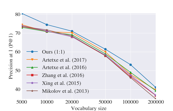
Figure 2: Bilingual dictionary induction results of our method and baselines for English–Italian with a 5,000 word seed lexicon across different vocabulary sizes.

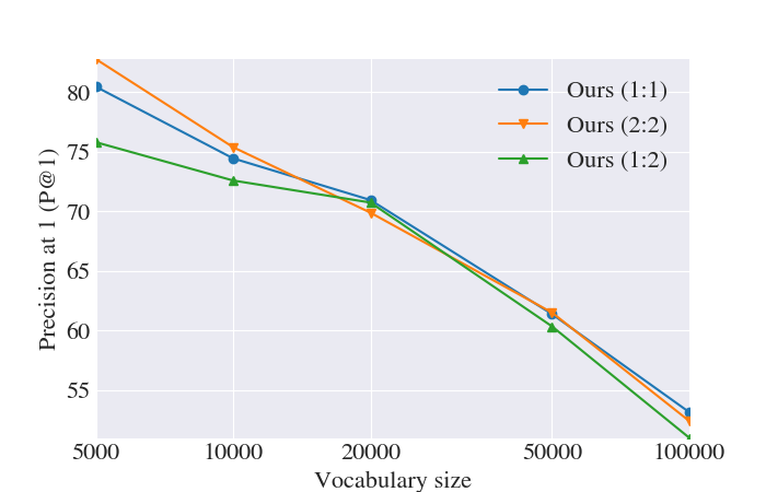
(a) English–Italian

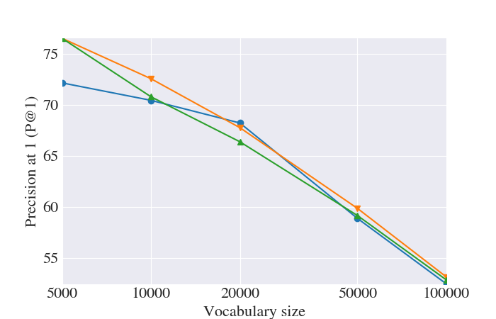
(b) English–German

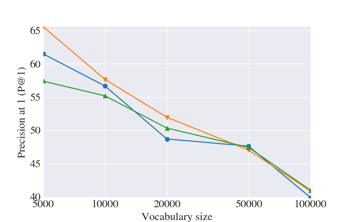
(c) English–Finnish

Figure 3: Bilingual dictionary induction results of our method with different priors using a 5,000 word seed lexicon across different vocabulary sizes.

The comparison approaches mostly perform similar, while our approach performs particularly well for the most frequent words in a language.

Different priors

An advantage of having an explicit prior as part of the model is that we can experiment with priors that satisfy different assumptions. Besides the 1:1 prior, we experiment with a 2:2 prior and a 1:2 prior. For the 2:2 prior, we create copies of the source and target words $V^{\prime}_{src}$ and $V^{\prime}_{trg}$ and add these to our existing set of vertices $V^{\prime}=(V_{trg}+V^{\prime}_{trg},V_{src}+V^{\prime}_{src})$. We run the Viterbi E-step on this new graph $G^{\prime}$ and merge matched pairs of words and their copies in the end. Similarly, for the 1:2 prior, which allows one source word to be matched to two target words, we augment the vertices with a copy of the source words $V^{\prime}_{src}$ and proceed as above. We show results for bilingual dictionary induction with different priors across different vocabulary sizes in Figure 3.

The 2:2 prior performs best for small vocabulary sizes. As solving the linear assignment problem for larger vocabularies becomes progressively more challenging, the differences between the priors become obscured and their performance converges.

Hubness problem

We analyze empirically whether the prior helps with the hubness problem. Following Lazaridou et al. (2015), we define the hubness $N_{k}(y)$ at $k$ of a target word $y$ as follows:

$$N_{k}(y)=|\{x\in Q\>|\>y\in\textit{NN}_{k}(x,G)\}|$$ (14)

where $Q$ is a set of query source language words and $\textit{NN}_{k}(x,G)$ denotes the $k$ nearest neighbors of $x$ in the graph $G$. In accordance with Lazaridou et al. (2015), we set $k=20$ and use the words in the evaluation dictionary as query terms. We show the target language words with the highest hubness using our method and Artetxe et al. (2017) for English–German with a 5,000 seed lexicon and the full vocabulary in Table 3.

Artetxe et al. (2017)	Ours (1:1)
luis (20)	gleichgültigkeit
	- `indifference' (14)
ungarischen	heuchelei
- `Hungarian' (18)	- `hypocrisy' (13)
jorge (17)	ahmed (13)
mohammed (17)	ideologie
	- `ideology' (13)
gewiß	eduardo (13)
- `certainly' (17)

Table 3: Hubs in English–German cross-lingual embedding space with degree of hubness. Non-name tokens are translated.

Hubs are fewer and occur less often with our method, demonstrating that the prior—to some extent—aids with resolving hubness. Interestingly, compared to Lazaridou et al. (2015), hubs seem to occur less often and are more meaningful in current cross-lingual word embedding models. For instance, the neighbors of `gleichgültigkeit' all relate to indifference and words appearing close to `luis' or `jorge' are Spanish names. This suggests that the prior might also be beneficial in other ways, e.g. by enforcing more reliable translation pairs for subsequent iterations.

Low-resource languages

Cross-lingual embeddings are particularly promising for low-resource languages, where few labeled examples are typically available, but are not adequately reflected in current benchmarks (besides the English–Finnish language pair). We perform experiments with our method with and without a rank constraint and Artetxe et al. (2017) for three truly low-resource language pairs, English–{Turkish, Bengali, Hindi}. We additionally conduct an experiment for Estonian-Finnish, similarly to Søgaard et al. (2018). For all languages, we use fastText embeddings Bojanowski et al. (2017) trained on Wikipedia, the evaluation dictionaries provided by Conneau et al. (2018), and a seed lexicon based on identical strings to reflect a realistic use case. We note that English does not share scripts with Bengali and Hindi, making this even more challenging. We show results in Table 4.

en-tr en-bn en-hi et-fi Artetxe et al. (2017) 28.93 0.87 2.07 30.18 Ours (1:1) 38.73 2.33 10.47 33.79 Ours (1:1, rank constr.) 42.40 11.93 31.80 34.78

Table 4: Bilingual dictionary induction results for English-{Turkish, Bengali, Hindi} and Estonian-Finnish.

Surprisingly, the method by Artetxe et al. (2017) is unable to leverage the weak supervision and fails to converge to a good solution for English-Bengali and English-Hindi. Our method without a rank constraint significantly outperforms Artetxe et al. (2017), while particularly for English-Hindi the rank constraint dramatically boosts performance.

Error analysis

To illustrate the types of errors the model of Artetxe et al. (2017) and our method with a rank constraint make, we query both of them with words from the test dictionary of Artetxe et al. (2017) in German and seek their nearest neighbours in the English embedding space. P@1 over the German-English test set is 36.38 and 39.18 for Artetxe et al. (2017) and our method respectively. We show examples where nearest neighbours of the methods differ in Table 5.

Similar to Kementchedjhieva et al. (2018), we find that morphologically related words are often the source of mistakes. Other common sources of mistakes in this dataset are names that are translated to different names and nearly synonymous words being predicted. Both of these sources indicate that while the learned alignment is generally good, it is often not sufficiently precise.

Query Gold Artetxe et al. (2017) Ours unregierbar ungovernable untenable uninhabitable nikolai nikolaj feodor nikolai memoranden memorandums communiqués memos argentinier argentinians brazilians argentines trostloser bleaker dreary dark-coloured umverteilungen redistributions inequities reforms modischen modish trend-setting modish tranquilizer tranquillizers clonidine opiates sammelsurium hotchpotch assortment mishmash demagogie demagogy opportunism demagogy andris andris rehn viktor dehnten halmahera overran stretched deregulieren deregulate deregulate liberalise eurokraten eurocrats bureaucrats eurosceptics holte holte threw grabbed reserviertheit aloofness disdain antipathy reaktiv reactively reacting reactive danuta danuta julie monika scharfblick perspicacity sagacity astuteness

Table 5: Example translations for German-English.

8 Related work

Cross-lingual embedding priors

Haghighi et al. (2008) first proposed an EM self-learning method for bilingual lexicon induction, representing words with orthographic and context features and using the Hungarian algorithm in the E-step to find an optimal 1:1 matching. Artetxe et al. (2017) proposed a similar self-learning method that uses word embeddings, with an implicit one-to-many alignment based on nearest neighbor queries. Vulić and Korhonen (2016) proposed a more strict one-to-many alignment based on symmetric translation pairs, which is also used by Conneau et al. (2018). Our method bridges the gap between early latent variable and word embedding-based approaches and explicitly allows us to reason over its prior.

Hubness problem

The hubness problem is an intrinsic problem in high-dimensional vector spaces Radovanović et al. (2010). Dinu et al. (2015) first observed it for cross-lingual embedding spaces and proposed to address it by re-ranking neighbor lists. Lazaridou et al. (2015) proposed a max-marging objective as a solution, while more recent approaches proposed to modify the nearest neighbor retrieval by inverting the softmax Smi (2017) or scaling the similarity values Conneau et al. (2018).

9 Conclusion

We have presented a novel latent-variable model for bilingual lexicon induction, building on the work of Artetxe et al. (2017). Our model combines the prior over bipartite matchings inspired by Haghighi et al. (2008) and the discriminative, rather than generative, approach inspired by Irvine and Callison-Burch (2013). We show empirical gains on six language pairs and theoretically and empirically demonstrate the application of the bipartite matching prior to solving the hubness problem.

References

- Smi (2017) 2017. Bilingual word vectors, orthogonal transformations and the inverted softmax. In Proceedings of ICLR.
- Adams and Zemel (2011) Ryan Prescott Adams and Richard S. Zemel. 2011. Ranking via Sinkhorn propagation. arXiv preprint arXiv:1106.1925.
- Artetxe et al. (2016) Mikel Artetxe, Gorka Labaka, and Eneko Agirre. 2016. Learning principled bilingual mappings of word embeddings while preserving monolingual invariance. Proceedings of the 2016 Conference on Empirical Methods in Natural Language Processing (EMNLP-16), pages 2289–2294.
- Artetxe et al. (2017) Mikel Artetxe, Gorka Labaka, and Eneko Agirre. 2017. Learning bilingual word embeddings with (almost) no bilingual data. In Proceedings of the 55th Annual Meeting of the Association for Computational Linguistics, pages 451–462.
- Artetxe et al. (2018) Mikel Artetxe, Gorka Labaka, and Eneko Agirre. 2018. Generalizing and Improving Bilingual Word Embedding Mappings with a Multi-Step Framework of Linear Transformations. In Proceedings of AAAI 2018.
- Bertsimas and Tsitsiklis (1997) D. Bertsimas and J.N. Tsitsiklis. 1997. Introduction to linear optimization. Athena Scientific.
- Bojanowski et al. (2017) Piotr Bojanowski, Edouard Grave, Armand Joulin, and Tomas Mikolov. 2017. Enriching Word Vectors with Subword Information. Transactions of the Association for Computational Linguistics.
- Brown et al. (1993) Peter F. Brown, Vincent J. Della Pietra, Stephen A. Della Pietra, and Robert L. Mercer. 1993. The mathematics of statistical machine translation: Parameter estimation. Computational Linguistics, 19(2):263–311.
- Camacho-Collados et al. (2015) José Camacho-Collados, Mohammad Taher Pilehvar, and Roberto Navigli. 2015. A Framework for the Construction of Monolingual and Cross-lingual Word Similarity Datasets. Proceedings of the 53rd Annual Meeting of the Association for Computational Linguistics and the 7th International Joint Conference on Natural Language Processing (Short Papers), (April 2016).
- Conneau et al. (2018) Alexis Conneau, Guillaume Lample, Marc'Aurelio Ranzato, Ludovic Denoyer, and Hervé Jégou. 2018. Word Translation Without Parallel Data. In Proceedings of ICLR 2018.
- Dinu et al. (2015) Georgiana Dinu, Angeliki Lazaridou, and Marco Baroni. 2015. Improving Zero-Shot Learning by Mitigating the Hubness Problem. ICLR 2015 Workshop track, pages 1–10.
- Fung (1995) Pascale Fung. 1995. Compiling bilingual lexicon entries from a non-parallel english-chinese corpus. In Third Workshop on Very Large Corpora.
- Gower and Dijksterhuis (2004) John C. Gower and Garmt B. Dijksterhuis. 2004. Procrustes problems. Oxford University Press.
- Grave et al. (2018) Edouard Grave, Armand Joulin, and Quentin Berthet. 2018. Unsupervised Alignment of Embeddings with Wasserstein Procrustes. arXiv preprint arXiv:1805.11222.
- Haghighi et al. (2008) Aria Haghighi, Percy Liang, Taylor Berg-Kirkpatrick, and Dan Klein. 2008. Learning Bilingual Lexicons from Monolingual Corpora. In Proceedings of ACL 2008, June, pages 771–779.
- Horn and Johnson (2012) Roger A. Horn and Charles R. Johnson. 2012. Matrix Analysis. Cambridge University Press.
- Irvine and Callison-Burch (2013) Ann Irvine and Chris Callison-Burch. 2013. Supervised bilingual lexicon induction with multiple monolingual signals. In Proceedings of the 2013 Conference of the North American Chapter of the Association for Computational Linguistics: Human Language Technologies, pages 518–523, Atlanta, Georgia. Association for Computational Linguistics.
- Jonker and Volgenant (1987) Roy Jonker and Anton Volgenant. 1987. A shortest augmenting path algorithm for dense and sparse linear assignment problems. Computing, 38(4):325–340.
- Kementchedjhieva et al. (2018) Yova Kementchedjhieva, Sebastian Ruder, Ryan Cotterell, and Anders Søgaard. 2018. Generalizing Procrustes Analysis for Better Bilingual Dictionary Induction. In Proceedings of CoNLL 2018.
- Klementiev et al. (2012) Alexandre Klementiev, Ann Irvine, Chris Callison-Burch, and David Yarowsky. 2012. Toward statistical machine translation without parallel corpora. In Proceedings of the 13th Conference of the European Chapter of the Association for Computational Linguistics, pages 130–140, Avignon, France. Association for Computational Linguistics.
- Koehn (2005) Philipp Koehn. 2005. Europarl: A parallel corpus for statistical machine translation. In MT Summit, volume 5, pages 79–86.
- Kuhn (1955) Harold W. Kuhn. 1955. The Hungarian method for the assignment problem. Naval Research Logistics (NRL), 2(1-2):83–97.
- Lazaridou et al. (2015) Angeliki Lazaridou, Georgiana Dinu, and Marco Baroni. 2015. Hubness and Pollution: Delving into Cross-Space Mapping for Zero-Shot Learning. Proceedings of the 53rd Annual Meeting of the Association for Computational Linguistics and the 7th International Joint Conference on Natural Language Processing, pages 270–280.
- Mayhew et al. (2017) Stephen Mayhew, Chen-Tse Tsai, and Dan Roth. 2017. Cheap translation for cross-lingual named entity recognition. In Proceedings of the 2017 Conference on Empirical Methods in Natural Language Processing, pages 2536–2545, Copenhagen, Denmark. Association for Computational Linguistics.
- Mena et al. (2018) Gonzalo Mena, David Belanger, Scott Linderman, and Jasper Snoek. 2018. Learning latent permutations with Gumbel-Sinkhorn networks. arXiv preprint arXiv:1802.08665.
- Mikolov et al. (2013a) Tomas Mikolov, Kai Chen, Greg Corrado, and Jeffrey Dean. 2013a. Distributed Representations of Words and Phrases and their Compositionality. In Advances in Neural Information Processing Systems.
- Mikolov et al. (2013b) Tomas Mikolov, Kai Chen, Greg Corrado, and Jeffrey Dean. 2013b. Efficient estimation of word representations in vector space. In International Conference on Learning Representations (ICLR) Workshop.
- Mikolov et al. (2013c) Tomas Mikolov, Quoc V. Le, and Ilya Sutskever. 2013c. Exploiting Similarities among Languages for Machine Translation.
- Neal and Hinton (1998) R. M. Neal and G. E. Hinton. 1998. A new view of the EM algorithm that justifies incremental, sparse and other variants. In M. I. Jordan, editor, Learning in Graphical Models, pages 355–368. Kluwer Academic Publishers.
- Radovanović et al. (2010) Milos Radovanović, Alexandros Nanopoulos, and Mirjana Ivanovic. 2010. Hubs in space: Popular nearest neighbors in high-dimensional data. Journal of Machine Learning Research, 11.
- Rapp (1995) Reinhard Rapp. 1995. Identifying word translations in non-parallel texts. In Proceedings of the 33rd Annual Meeting of the Association for Computational Linguistics, pages 320–322, Cambridge, Massachusetts, USA. Association for Computational Linguistics.
- Ruder et al. (2018) Sebastian Ruder, Ivan Vulić, and Anders Søgaard. 2018. A survey of cross-lingual word embedding models. Journal of Artificial Intelligence Research.
- Samdani et al. (2012) Rajhans Samdani, Ming-Wei Chang, and Dan Roth. 2012. Unified expectation maximization. In Proceedings of the 2012 Conference of the North American Chapter of the Association for Computational Linguistics: Human Language Technologies, pages 688–698, Montréal, Canada. Association for Computational Linguistics.
- Schönemann (1966) Peter H. Schönemann. 1966. A generalized solution of the orthogonal Procrustes problem. Psychometrika, 31(1):1–10.
- Søgaard et al. (2018) Anders Søgaard, Sebastian Ruder, and Ivan Vulić. 2018. On the Limitations of Unsupervised Bilingual Dictionary Induction. In Proceedings of ACL 2018.
- Valiant (1979) Leslie G. Valiant. 1979. The complexity of computing the permanent. Theoretical Computer Science, 8(2):189–201.
- Villani (2008) Cédric Villani. 2008. Optimal transport: Old and new, volume 338. Springer Science & Business Media.
- Volgenant (1996) A Volgenant. 1996. Linear and semi-assignment problems: a core oriented approach. Computers & Operations Research, 23(10):917–932.
- Vulić and Korhonen (2016) Ivan Vulić and Anna Korhonen. 2016. On the Role of Seed Lexicons in Learning Bilingual Word Embeddings. Proceedings of ACL, pages 247–257.
- West (2000) Douglas B. West. 2000. Introduction to Graph Theory, 2 edition. Prentice Hall.
- Xing et al. (2015) Chao Xing, Chao Liu, Dong Wang, and Yiye Lin. 2015. Normalized Word Embedding and Orthogonal Transform for Bilingual Word Translation. NAACL-2015, pages 1005–1010.
- Zhang et al. (2016) Yuan Zhang, David Gaddy, Regina Barzilay, and Tommi Jaakkola. 2016. Ten Pairs to Tag – Multilingual POS Tagging via Coarse Mapping between Embeddings. In Proceedings of NAACL-HLT 2016, pages 1307–1317.