Physical interpretation of the canonical ensemble for long-range interacting systems in the absence of ensemble equivalence

Abstract

In systems with long-range interactions, since energy is a non-additive quantity, ensemble inequivalence can arise: it is possible that different statistical ensembles lead to different equilibrium descriptions, even in the thermodynamic limit. The microcanonical ensemble should be considered the physically correct equilibrium distribution as long as the system is isolated. The canonical ensemble, on the other hand, can always be defined mathematically, but it is quite natural to wonder to which physical situations it does correspond. We show numerically and, in some cases, analytically, that the equilibrium properties of a generalized Hamiltonian mean-field model in which ensemble inequivalence is present are correctly described by the canonical distribution in (at least) two different scenarios: a) when the system is coupled via local interactions to a large reservoir (even if the reservoir shows, in turn, ensemble inequivalence) and b) when the mean-field interaction between a small part of a system and the rest of it is weakened by some kind of screening.

I Introduction

Equilibrium statistical mechanics provides a very accurate description of the statistical features of systems with many particles. Relevant results can be derived when only short-range interactions are involved and the thermodynamic limit is considered; among them, equivalence of statistical ensembles covers a prominent role, since it allows the computation of averages for macroscopic observables according to different statistical descriptions Huang (1988). From a technical point of view it relies on the validity of the law of large numbers and of the central limit theorem, on the results of large deviations theory, but also on the concavity of thermodynamic potentials Touchette (2009). More difficult cases are:

• systems at the critical point where also spatially far parts are strongly interacting, so that the central limit theorem cannot be used (see e.g. Ma (1985); Sethna (2005));

• systems with few degrees of freedom Seifert (2012); Cerino et al. (2015); Puglisi et al. (2017);

• systems with long-range interactions, in which potentials decay not faster than $r^{-d}$, where $r$ is the distance and $d$ the spatial dimension Dauxois et al. (2002).

The latter case includes rather interesting physical problems, e.g. in plasma, hydrodynamics, self gravitating systems and lasers Dauxois et al. (2002). In addition, all systems in which the elements interact via a mean field also belong to this category.

In systems with long-range interactions the equivalence of statistical ensembles is not guaranteed: in particular there are rigorous results for Hamiltonian models with mean field interactions, showing that the thermodynamic potentials can be non convex; this is due to the non-additivity of energy Campa et al. (2009).,graphicx,enumerate As a consequence, the canonical and microcanonical ensembles can give different results, i.e. the average of a macroscopic observable $A$ is sensitive to the choice of the probability density function:

$$\langle A\rangle_{m}\neq\langle A\rangle_{c}\,.$$

In other words, fixing the energy $E$ of a system does not always lead to the same average one gets by fixing its temperature to the corresponding value $T(E)\equiv\left(\frac{\partial S}{\partial E}\right)^{-1}$, where $S$ is the microcanonical entropy. These results are rather clear from a mathematical point of view, but their physical meaning may appear not completely obvious, due to some potential sources of confusion in the “operative definition” of the canonical ensemble for long-range interacting systems.

Microcanonical ensemble always possess a transparent physical interpretation, since it describes the statistical properties of isolated Hamiltonian systems. The canonical ensemble, on the other hand, should be used for systems at fixed temperature; it characterises, in particular, systems of Brownian particles, where the stochastic forces and the dissipation provide a constraint on the temperature: such mechanism usually originates from the interactions of the particles with another system (of a different nature) which acts as a stochastic thermal bath. The above discussion is valid regardless of the range of the potential, and both microcanonical and canonical ensemble have been extensively studied also for systems showing long-range interactions Chavanis (2006). Clearly, every Hamiltonian system (which is described by the microcanonical ensemble as long as it is isolated) can be related to a Brownian system (which is instead correctly described by the canonical ensemble): notable examples are the relation between stellar systems and self-gravitating Brownian particles Sire and Chavanis (2004) and that between the Hamiltonian Mean Field model Antoni and Ruffo (1995) and the Brownian Mean Field model Chavanis (2014).

As far as Hamiltonian systems with only short-range interactions are considered, the canonical ensemble can be defined in a different way: it is generally possible to observe the statistical behaviour of a small number of degrees of freedom and regard the rest of the system as a thermal bath constraining the temperature of such small portion. The procedure can be found on textbooks Huang (1988) and requires that the Hamiltonian term which represents the reciprocal interaction is negligible in the thermodynamic limit. In this case the temperature is fixed in a natural way, even in absence of an “external” reservoir. As soon as long-range interactions are involved, the above procedure cannot be applied: “surface contributions” to the energy of the small part, due to the interactions with the rest of the system, are no more negligible (i.e. energy is a non-additive quantity) and canonical ensemble cannot be defined in this way.

In past years some authors claimed that systems with long-range interactions should be only described by the microcanonical ensemble Gross (2002, 2002). It has also been pointed out that for self-gravitating systems canonical ensemble could be only defined at a formal level Padmanabhan (1990). In the light of the above, other people stressed instead the role of canonical ensemble in describing systems of Brownian particles coupled to external baths Chavanis (2002). Operative protocols have also been studied in order to model a “physical” thermal reservoir in numerical simulations, and their effects on the system have been compared to those of Nosé-Hoover thermostats and Monte-Carlo integration schemes in non-equilibrium conditions Baldovin and Orlandini (2006, 2007); Baldovin et al. (2009).

In this paper we address the problem of the physical meaning of canonical ensemble when mean-field interacting systems with non-equivalence of ensembles are involved; in particular, we show by numerical simulations that the canonical ensemble is the only one that provides the correct equilibrium behavior

• when the system is coupled via small local interactions to a large thermal bath;

• when the (mean-field) interaction between a small part of the system and the rest of it is very weak.

In the following we will study the Generalized Hamiltonian Mean Field (GHMF) model introduced in Ref. de Buyl et al. (2005). This system is a generalization of the well-known Hamiltonian Mean Field model Antoni and Ruffo (1995); it is composed of $N$ rotators whose Hamiltonian (with an additive constant) is:

$$H_{N}=\sum_{i=1}^{N}\frac{p_{i}^{2}}{2}+N\left[\frac{J}{2}(1-m^{2})+\frac{K}{4}(1-m^{4})\right]$$ (1)

where $J$ and $K$ are constant parameters, $m$ is the intensity of a magnetization defined as

$$m=\sqrt{m_{x}^{2}+m_{y}^{2}}\quad\quad m_{x}=\frac{1}{N}\sum_{i=1}^{N}\sin\theta_{i}\quad\quad m_{y}=\frac{1}{N}\sum_{i=1}^{N}\cos\theta_{i}\,$$ (2)

and $\{\theta_{i},p_{i}\}\quad i=1,...,N$ are canonical variables. The statistical properties of GHMF model can be analytically studied using large-deviations techniques Campa et al. (2009). This approach shows that an isolated system can be characterized by negative specific heat $\partial\varepsilon/\partial T<0$ (where $\varepsilon$ is the specific energy and $T$ the system’s temperature) in a certain energy range for suitable choices of $J$ and $K$. Therefore, microcanonical and canonical ensembles are not equivalent, so that the graph of $T(\varepsilon)$ in the latter description is not the inverse of $\varepsilon(T)$ in the former (it is necessary to introduce a Maxwell construction, since a first order phase transition occurs in the canonical ensemble).

The paper is organized as follows. Section II is devoted to the investigation of different protocols to build a “physical” thermal reservoir for the GHMF model. We show by numerical simulations that when the system is coupled to the thermal bath by local interactions, its thermodynamic behavior is described by the canonical ensemble, and ensemble inequivalence is clearly evident; this is also true in the not completely trivial case in which the reservoir is a GHMF system as well (therefore exhibiting negative specific heat). In Section III the related problem of the equilibrium properties of a weakly interacting portion of a GHMF system is investigated. We introduce a parameter $\lambda$ which tunes the mean-field interaction between two portions of the system: $\lambda$ determines how much each of the two subsystems “feels” the mean-field effect of the other, varying between 0 (two isolated GHMF systems) and 1 (a unique GHMF system resulting from the complete mean-field interaction of the two parts). The equilibrium behavior of a small portion of the system as a function of $\lambda$ is analyzed using large deviation theory and molecular dynamics simulations: in the $\lambda\ll 1$ limit, the canonical description is recovered.

In Section IV we briefly sketch our final remarks.

II Locally coupled “thermal baths” for systems with non-equivalence of ensembles

In the following we consider three different ways of building a “thermal reservoir” in numerical simulations. Each reservoir is coupled to a small GHMF system (1) with $J=1$, $K=10$. It has been shown Patelli and Ruffo (2014) that this choice of the parameters leads to first-order phase transitions in both microcanonical and canonical ensembles; the latter is a direct consequence of the non-equivalence.

In this Section we consider “local” couplings: each particle of the system interacts with only one particle of the bath. The coupling potential is given by an Hamiltonian term $\lambda V_{coup}(\delta)$, where $\lambda$ is a (small) constant which indicates the strength of the interaction and $V_{coup}$ is a function of the angular distance $\delta$ between the two particles. We choose:

$$V_{coup}(\delta)=A-B\cos\delta-C\cos^{2}\delta$$ (3)

with $A=J/2+3K/8$, $B=J/2+K/4$ and $C=K/8$, which is the interaction term of Hamiltonian (1) when $N=2$. There is no particular reason to make this choice for $V_{coup}(\delta)$, and the results should be quite independent of its form, provided that its contribution to the total Hamiltonian is negligible.

Unless otherwise specified, molecular dynamics simulations reported in the present and in the following Section are performed using a second-order Velocity Verlet scheme, in which we take time steps short enough to get energy fluctuations of order $O(\Delta E/E)\approx 10^{-5}$. Since we are interested in long-range interacting models at equilibrium, we compute averages, as far as we can, after thermalization, i.e. after the system has departed from possible metastable states. Such process can take very long times, depending on the total number of particles $N$ (see Ref. Yamaguchi et al. (2004); de Buyl et al. (2011); Pakter and Levin (2011)): for this reason, in our simulations we choose relatively small values of $N$ (but still in the limit $N\gg 1$), namely $N\approx O(10^{2})$ for the system and $N_{res}\approx O(10^{3})$ for the reservoir. Initial values for positions and momenta are chosen according to Gaussian distributions, and then rescaled in order to get the needed total energy; however we stress that, since averages are computed after long thermalization times, our equilibrium results should hold independently of the particular choice of initial conditions.

II.1 Stochastic heat-bath

First we study a bath composed of $N_{res}$ particles held at a fixed $T$ by a stochastic term in its evolution equation: this term should model the effect of several “collisions” occurring on the rotators of the reservoir. We choose $N_{res}=N$, where $N$ is the number of elements in the analyzed system, so that every particle of the system is coupled to exactly one particle of such reservoir; consequently, the complete Langevin equation describing the motion of a single rotator in the bath (identified by an angular position $\xi_{i}$ and a momentum $\pi_{i}$) reads:

$$\begin{cases}\dot{\xi}_{i}=\pi_{i}\\ \dot{\pi_{i}}=-\frac{1}{\tau}\pi_{i}+\sqrt{\frac{2T}{\tau}}\eta_{i}(t)-\lambda\frac{d}{d\xi_{i}}V_{coup}(\theta_{i}-\xi_{i})\end{cases}$$ (4)

where $\tau$ is a characteristic time of the system, $\eta_{i}(t)$ is a delta-correlated Gaussian noise with zero mean such that $\langle\eta_{i}(t)\eta_{j}(t^{\prime})\rangle=\delta_{ij}\delta(t-t^{\prime})$ and $\theta_{i}$ is the angular position of the coupled particle in the system. Here the Boltzmann’s constant is 1. On the other hand, the motion equations for a particle of the system are:

$$\begin{cases}\dot{\theta}_{i}=p_{i}\\ \dot{p}_{i}=-(J+Km^{2})(m_{x}\sin\theta_{i}-m_{y}\cos\theta_{i})-\lambda\frac{d}{d\theta_{i}}V_{coup}(\theta_{i}-\xi_{i})\,.\end{cases}$$ (5)

All simulations follow the protocol below:

1. during the time interval $0<t<t_{0}$ the system is decoupled from the reservoir ($\lambda=0$) and it evolves deterministically;

2. the temperature $T$ of the system is computed by averaging the observable $p_{i}^{2}$ over all particles for $0<t<t_{0}$;

3. the temperature of the bath is set equal to $T$;

4. for $t>t_{0}$ the coupling is switched on ($\lambda>0$) and the total system evolves according to the stochastic position Verlet algorithm for Langevin equations discussed in Ref. Melchionna (2007).

The process is repeated for several starting specific energy $\varepsilon$ of the system.

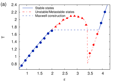
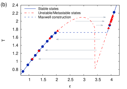
Figure 1: $T(\varepsilon)$ vs $\varepsilon$ for the GHMF model interacting with a stochastic thermal bath, before (a) and after (b) the coupling. Points have been marked in different ways according to the initial specific energy. All simulations have been performed with the following parameters: $N=100$, $\lambda=0.02$, $\tau=20$, $t_{0}=8\cdot 10^{4}$. Averages in the second figure have been computed over a time interval $\Delta t=1.6\cdot 10^{6}$, starting at $t=1.2\cdot 10^{6}\gg t_{0}$.

The above setting could sound quite unphysical; we remark however that its study is certainly useful in order to check wether the system can actually reach the correct equilibrium distribution through the dynamics: such possibility could be questioned if the system starts from metastable states, since in this case thermalization times are potentially huge. In addition, this stochastic approach can give useful insight about the typical waiting times to be expected in the deterministic simulations.

The results are shown in Fig. 1, in which each point represents a simulation. As long as the system is isolated, its $T(\varepsilon)$ dependence is given by the microcanonical caloric curve, which consists not only of stable states, but also of unstable and metastable ones Campa et al. (2009), i.e. states whose $\varepsilon$ does not minimize free energy when $T$ is fixed. This is quite evident in the second graph of Fig. 1: when the system is coupled to the reservoir, after some time it reaches the “true” equilibrium state at the same temperature (which is fixed by the bath) but with a different specific energy. For metastable states this process can take, as it is well known, very long times even for a relatively small number of particle, and this explains the residual point in the “forbidden” branch of the curve.

We stress that this simple stochastic approach clearly shows that, at least for this particular choice of the physical parameters, dynamics does select the correct equilibrium distribution (in accessible comuputational times). This consideration is very important, since it suggests the possibility of similar results also in deterministic simulations.

II.2 Hamiltonian reservoir with short-range interactions

The following protocol simulates a thermal bath by using an Hamiltonian system. In a more general fashion it has been already introduced in Ref. Baldovin and Orlandini (2006) in order to study the non equilibrium behavior of the Hamiltonian Mean Field model (system (1) with $K=0$). The reservoir consists of a chain of $N_{res}\gg N$ first-neighbors rotators; $N$ of them, randomly chosen, are in turn coupled to the system, trough the $\lambda V_{coup}(\delta)$ pair potential (see Eq. (3)). Let us remark that in Ref. Baldovin and Orlandini (2006) each particle of the system was in contact with $S$ particles in the bath; choosing $S\propto N^{-1/2}$, one reproduces the “surface-like” effect in the thermodynamic limit. Here we are considering the case $S=1$, with the additional constraint that each rotator of the reservoir can be coupled to no more than one particle of the system.
The total Hamiltonian is:

$$H_{tot}=H_{N}(\{\theta_{i},p_{i}\})+\sum_{i=1}^{N_{res}}\frac{\pi_{i}^{2}}{2}+\gamma\sum_{i=1}^{N_{res}+1}(1-\cos(\xi_{i}-\xi_{i-1}))+\lambda\sum_{i=1}^{N}V_{coupl}(\xi_{r_{i}}-\theta_{i})$$ (6)

where $\{\xi_{i},\pi_{i}\}$ are the coordinates of the particles in the reservoir ($\xi_{0}\equiv\xi_{N+1}\equiv 0$) and $\{r_{i}\}$ are distinct integers randomly chosen in the interval $[1,N_{res}]$.

Figure 2: $T(\varepsilon)$ vs $\varepsilon$ for the GHMF model interacting with a Hamiltonian reservoir with short-range interactions. Parameters: $N=80$, $N_{res}=800$, $\gamma=10$, $\lambda=0.02$. Averages have been computed over a time interval $\Delta t=4\cdot 10^{5}$, after $t=8\cdot 10^{5}$ time units.

Simulating the total Hamiltonian at different energies $E_{tot}$, we can sketch the $T(\varepsilon)$ dependence for the GHMF system. Fig. 2 shows that also in this case, once equilibrium has been reached, canonical ensemble provides the correct statistical description (besides some long-lasting metastable states). As already noticed in Ref. Baldovin and Orlandini (2006), thermal equilibrium is not “assumed” by the simulation protocol (as it happens when stochastic terms are involved), instead it is reached by the system in a rather physical way.

II.3 GHMF reservoir

It could be not completely obvious what does it happen when the reservoir is constituted by another, larger, GHMF system. In Ref. Ramírez-Hernández et al. (2008) violations of the zero-th law of Thermodynamics have been found for a long-range interacting model in which, as in the GHMF, statistical ensembles are not equivalent; it has been shown that, if two isolated systems with equal size share the same temperature $T_{1}$, but their specific heat is negative, they will reach a different temperature $T_{2}$ when coupled each other.

It can be easily seen, trough a microcanonical approach quite similar to the one used in Ref. Ramírez-Hernández et al. (2008), that this is not the case when the ratio $N_{2}/N_{1}$ between the sizes of the two systems is very high: in such situation the temperature of the larger one does not change significantly, while, as expected, the thermodynamic behavior of the smaller one is described by the canonical ensemble. Indeed, if one defines $\alpha\equiv N_{1}/(N_{1}+N_{2})$ and indicates by $\varepsilon_{1}$ and $\varepsilon_{2}$ the specific energies of the two systems, the most probable value of $\varepsilon_{1}$ at fixed total energy $E$ can be computed in general by maximizing the total entropy

$$s_{tot}(\varepsilon_{1},\varepsilon_{2})=\alpha s(\varepsilon_{1})+(1-\alpha)s(\varepsilon_{2})$$ (7)

with the constraint $\varepsilon_{tot}\equiv E/(N_{1}+N_{2})=\alpha\varepsilon_{1}+(1-\alpha)\varepsilon_{2}$, where $s(\varepsilon)$ is the entropy of the GHMF model. Critical points of entropy (7) are obtained for values of $\varepsilon_{1}$ such that the temperatures of the two subsystems are equal, i.e.:

$$s^{\prime}(\varepsilon_{1})-s^{\prime}\left(\frac{\varepsilon_{tot}-\alpha\varepsilon_{1}}{1-\alpha}\right)=0\,$$ (8)

Anyway, if different solutions $\varepsilon_{1}^{(n)}$, $n=1,2,...$ of Eq. (8) do exist (i.e. if $s(\varepsilon)$ is not a strictly concave function), the one that corresponds to the stable equilibrium, $\varepsilon_{1}^{*}$, must fulfill

$$s_{tot}\left(\varepsilon_{1}^{*},\frac{\varepsilon_{tot}-\alpha\varepsilon_{1}^{*}}{1-\alpha}\right)\geq s_{tot}\left(\varepsilon_{1}^{(n)},\frac{\varepsilon_{tot}-\alpha\varepsilon_{1}^{(n)}}{1-\alpha}\right)\;\forall n\,.$$ (9)

The above inequality can be studied in the $\alpha\ll 1$ limit with a first-order expansion. One gets

$$\alpha\left[s(\varepsilon_{1}^{*})-s(\varepsilon_{1}^{(n)})\right]\geq s^{\prime}(\varepsilon_{tot})\alpha(\varepsilon_{tot}-\varepsilon^{(n)})-s^{\prime}(\varepsilon_{tot})\alpha(\varepsilon_{tot}-\varepsilon_{1}^{*})$$ (10)

which immediately leads to the integral condition

$$\int_{\varepsilon_{1}^{*}}^{\varepsilon_{1}^{(n)}}T^{-1}(\varepsilon^{\prime})d\varepsilon^{\prime}\leq T^{-1}(\varepsilon_{tot})(\varepsilon_{1}^{(n)}-\varepsilon_{1}^{*})\;\forall n\,$$ (11)

because of the relation $T^{-1}(\varepsilon)\equiv s^{\prime}(\varepsilon)$. The above condition is nothing but the Maxwell construction; one can therefore conclude that in the limit $\alpha\ll 1$, i.e. when it is possible to identify a reservoir composed of $N_{res}=N_{2}$ particles and a small system made of $N=N_{1}$ rotators coupled to it, with $N\ll N_{res}$, the equilibrium behavior of the second is described by the canonical ensemble at temperature $T(\varepsilon_{tot})$. Since

$$\varepsilon_{2}=\frac{\varepsilon_{tot}-\alpha\varepsilon_{1}}{1-\alpha}\approx\varepsilon_{tot}+\alpha(\varepsilon_{tot}-\varepsilon_{1})+O(\alpha^{2})$$ (12)

it is also proved that $T(\varepsilon_{tot})\approx T(\varepsilon_{2})+O(\alpha)$ (if $\varepsilon_{tot}$ is not too close to a microcanonical phase transition), i.e. the temperature of the small system is determined by the one of the reservoir, as expected, even if the reservoir is in an “unstable” state with negative specific heat.
The above considerations can be tested by numerical simulations on a system of the kind:

$$H_{tot}=H_{N}(\{\theta_{i},p_{i}\})+H_{N_{res}}(\{\xi_{i},\pi_{i}\})+\lambda\sum_{i=1}^{N}V_{coup}(\theta_{i}-\xi_{i})$$ (13)

where $H_{N}$ and $V_{coup}$ have been defined in Eq. (1) and (3). In Fig. 3, panel (a), we see that the $T(\varepsilon)$ dependence for the small system is in a rather good agreement with the theoretical prediction, where $T$ is estimated by the average $\langle p_{i}^{2}\rangle$ on the $N$ particles of the small system itself. Not surprisingly, in some cases the system is trapped in a metastable state. As expected, the reservoir (inset) can assume every specific energy at equilibrium, even those leading to negative specific heat. Panel (b) of Fig. 3 shows the relation between the specific energies of the bath ($\varepsilon_{2}$) and that of the system ($\varepsilon_{1}$), compared to the theoretical curve.

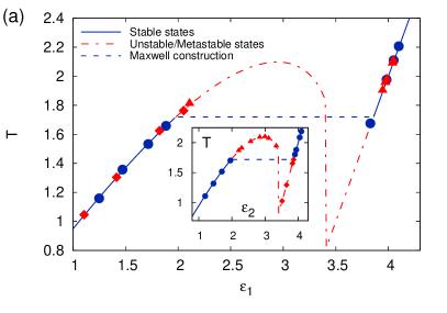
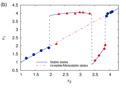
Figure 3: Case of a GHMF system coupled to a GHMF reservoir. (a) Caloric curve for the system, $T(\varepsilon_{1})$ vs $\varepsilon_{1}$, (main plot) where $T$ is estimated by a direct average $\langle p_{i}^{2}\rangle$ on the particles of the system; the caloric curve for the reservoir, $T(\varepsilon_{2})$ vs $\varepsilon_{2}$, is also shown (inset). (b) Relation between $\varepsilon_{1}$ and $\varepsilon_{2}$. Points are marked in different ways according to the average energy of the reservoir in the considered simulation. Parameters: $N=80$, $N_{res}=800$, $\lambda=0.02$. Averages have been computed over a time interval $\Delta t=4.0\cdot 10^{5}$.

III Equilibrium behavior of a weakly interacting portion of a mean-field system

Let us consider the (quite reasonable) situation in which a mean-field interacting system is split into two parts $\mathcal{S}_{1}$ and $\mathcal{S}_{2}$, in such a way that the effective mean field acting on each particle of $\mathcal{S}_{1}$ depends strongly on the degrees of freedom $\mathbf{X}_{1}$ of $\mathcal{S}_{1}$ itself and weakly on those of $\mathcal{S}_{2}$ (i.e. $\mathbf{X}_{2}$), and vice versa. In real physical systems this could be obtained by some kind of screening between the two parts, or by simply distancing them to a range in which mean field interactions are no more a valid approximation.

Consider the case of GHMF model, and call $\mathbf{m}_{1}(\mathbf{X}_{1})$ and $\mathbf{m}_{2}(\mathbf{X}_{2})$ the magnetization vectors of the two subsystems, whose components are defined according to Eq. (2). It is reasonable to assume that the effective fields acting on $\mathcal{S}_{1}$ and $\mathcal{S}_{2}$ can be described by

$$\begin{cases}\mathbf{m}_{1}^{*}(\mathbf{X}_{1},\mathbf{X}_{2})=(1-\lambda)\mathbf{m}_{1}(\mathbf{X}_{1})+\lambda\mathbf{m}(\mathbf{X}_{1},\mathbf{X}_{2})\\ \mathbf{m}_{2}^{*}(\mathbf{X}_{1},\mathbf{X}_{2})=(1-\lambda)\mathbf{m}_{2}(\mathbf{X}_{2})+\lambda\mathbf{m}(\mathbf{X}_{1},\mathbf{X}_{2})\end{cases}$$ (14)

where $\mathbf{m}(\mathbf{X}_{1},\mathbf{X}_{2})$ is the mean field of the total system without splitting and $\lambda\in[0,1]$ is a real parameter which quantifies the interaction, so that $\lambda=0$ when the subsystems are completely isolated and $\lambda=1$ when there’s no screening at all. The total Hamiltonian reads

$$H_{tot}(\mathbf{X}_{1},\mathbf{X}_{2})=\sum_{i=1}^{N_{1}+N_{2}}\frac{p_{i}^{2}}{2}+N_{1}u(m_{1}^{*})+N_{2}u(m_{2}^{*})$$ (15)

where $N_{1}$ and $N_{2}$ are the number of particles in $\mathcal{S}_{1}$ and $\mathcal{S}_{2}$, and

$$u(x)\equiv\frac{J}{2}(1-x^{2})+\frac{K}{4}(1-x^{4})\,.$$

The equilibrium properties for given values of $\lambda$ and $\alpha\equiv N_{1}/(N_{1}+N_{2})$ of this Hamiltonian system can be derived exactly, in the thermodynamic limit, by using large deviations techniques (see Appendix).

Let us note that, since long-range interactions are involved, one can introduce different definitions for the energy of $\mathcal{S}_{1}$, depending on which extent the non-negligible interactions with $\mathcal{S}_{2}$ are taken into account. In this context, anyway, the following microcanonical average

$$E_{1}=\langle\sum_{i=1}^{N_{1}}\frac{p_{i}^{2}}{2}+N_{1}u(m_{1}^{*})\rangle$$ (16)

seems to be a quite reasonable choice.

Let us focus first on the $\lambda\ll 1$ case. Eq. (15) can be rewritten in the form

$$H_{tot}(\mathbf{X}_{1},\mathbf{X}_{2})=H_{N_{1}}(\mathbf{X}_{1})+H_{N_{2}}(\mathbf{X}_{1})+\lambda H_{int}(\mathbf{X}_{1},\mathbf{X}_{2})$$ (17)

where $H_{N}$ is the GHMF model Hamiltonian (1) for a system of $N$ particles and the $\lambda H_{int}$, whose average is negligible with respect to those of $H_{N_{1}}$ and $H_{N_{2}}$, includes all interactions terms between the two systems. All interactions in this system are long-range; nonetheless, in this particular limit, we recover the conditions that are needed in the well-known derivation of canonical ensemble from a microcanonical description. Assuming that ergodicity holds, in this limit one expects a thermodynamic behavior quite similar to those that have been discussed in Section II.

In the opposite limit, namely $\lambda\lesssim 1$, the energy range in which $m^{*}_{1}\neq m^{*}_{2}$ gradually shrinks. Above certain critical value $\bar{\lambda}(\alpha)$, condition $m^{*}_{1}=m^{*}_{2}$ (or, equivalently, $m_{1}=m_{2}$) always holds at equilibrium, and for $\lambda=1$, the $T(\varepsilon_{1})$ curve will coincide with the microcanonical one, as long as the above definition of energy is considered.

In Fig. 4 the two situations are shown for a fixed (small) value of $\alpha$, and numerical simulations are compared to analytical calculations.

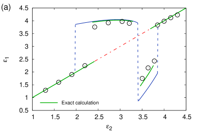
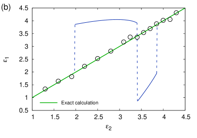
Figure 4: Specific energy $\varepsilon_{1}$ of the small portion vs specific energy $\varepsilon_{2}$ of the large one, for $\lambda=0.05$ (a) and $\lambda=0.1$ (b). Green solid lines stand for the exact solutions computed as described in the Appendix. Equilibrium behavior of the system in the microcanonical (red) and canonical (blue) ensembles are also shown for comparison. Parameters: $N_{1}=50$, $N_{2}=800$ ($\alpha=1/17$), $\lambda=0.02$. Averages have been computed over time intervals $\Delta t=3.5\cdot 10^{7}$ (left) and $\Delta t=10^{7}$ (right).

As far as mean field interactions are concerned, some general considerations about the thermodynamics of a small piece $\mathcal{S}_{1}$ of the total system $\mathcal{S}_{tot}$ can be outlined. If definition (16) is considered, the caloric curve of $\mathcal{S}_{1}$ is the same of an isolated system: in particular negative specific heat can be observed, because of the action of the mean field of $\mathcal{S}_{tot}$ which keeps the subsystem in unstable energy regions; when the effect of the total mean field is weakened trough some screening, but not enough to prevent heat exchange between the two subsystems, unstable and metastable states are no more accessible for $\mathcal{S}_{1}$ and the canonical description is recovered in the limit.
On the other hand, if one defines the energy of the subsystem as the sum of all terms of the total Hamiltonian which depend on $\mathbf{X}_{1}$ only, the caloric curve tends to the one of the ideal gas, since average kinetic energy is of order $\alpha N$ and the average potential energy is of order $\alpha^{2}N$, because of Kac’s prescription Campa et al. (2009).

IV Final remarks

In this paper we have investigated several different physical situations in which the equilibrium behavior of a long-range interacting system with ensemble inequivalence is described by the canonical distribution. The aim of such approach is to clarify the physical interpretation of this statistical ensemble, which can always be defined from a mathematical point of view.

First we have studied, by numerical simulations, the case in which a small system is in contact with a large reservoir; then we have analyzed the equilibrium behavior of a small portion of a mean-field system, partially isolated from the rest of it by some kind of screening. In both cases, the studied degrees of freedom interact weakly with the remaining part of the system; nonetheless, energy can still be exchanged, so that the larger part of the system determines the temperature of the smaller one. This is indeed a physically relevant way to construct the canonical ensemble.

Our results show that the canonical distribution is physically meaningful also when inequivalence of statistical ensemble is present, as far as the above conditions hold. Since such assumptions are verified in rather interesting cases, the usage of canonical ensemble for long-range interacting systems seems quite natural and fully justified from a physical point of view.

V Appendix

In this Appendix we use large deviations techniques to investigate the equilibrium behavior, in the thermodynamic limit, of the Hamiltonian system (15). Large deviations are a well-known tool for the study of mean-field systems Patelli and Ruffo (2014). This approach can be used if the Hamiltonian depends only on $n\ll N$ mean quantities $\mu_{j}(\mathbf{X})$ with the form $\mu_{j}=\sum_{i=1}^{N}g(q_{i},p_{i})$, $j=1,...,n$, or if the energy contribution of other terms is negligible in the thermodynamic limit. With the above assumptions it is possible to compute the so-called entropy of macrostates

$$\bar{s}(\bar{\mu}_{1},...,\bar{\mu}_{n})\equiv\frac{1}{N}\ln\int d\mathbf{X}\,\delta(\mu_{1}(\mathbf{X})-\bar{\mu}_{1})\delta(\mu_{2}(\mathbf{X})-\bar{\mu}_{2})...\delta(\mu_{n}(\mathbf{X})-\bar{\mu}_{n})\,,$$ (18)

which is maximal in the equilibrium macrostates of the microcanonical ensemble. Even if Hamiltonian (15) is not in the requested form, its $\bar{s}(\bar{\mu}_{1},...,\bar{\mu}_{n})$ can be easily computed. Indeed, Hamiltonian (15) can be written as

$$H_{tot}(\mathbf{X}_{1},\mathbf{X}_{2})=\bar{H}(\kappa_{1},m_{1x},m_{1y},\kappa_{2},m_{2x},m_{2y})=\bar{H}(\mathbf{w}_{1},\mathbf{w}_{2})$$ (19)

where

$$\kappa_{1} =\frac{1}{N_{1}}\sum_{i=1}^{N_{1}}p_{i}^{2} m_{1x} =\frac{1}{N_{1}}\sum_{i=1}^{N_{1}}\cos\theta_{i} m_{1y} =\frac{1}{N_{1}}\sum_{i=1}^{N_{1}}\sin\theta_{i}$$

$$\kappa_{2} =\frac{1}{N_{2}}\sum_{i=N_{1}+1}^{N_{1}+N_{2}}p_{i}^{2} m_{2x} =\frac{1}{N_{2}}\sum_{i=N_{1}+1}^{N_{1}+N_{2}}\cos\theta_{i} m_{2y} =\frac{1}{N_{2}}\sum_{i=N_{1}+1}^{N_{1}+N_{2}}\sin\theta_{i}$$

and

$$\mathbf{w}_{1}=(\kappa_{1},m_{1x},m_{1y})\quad\quad\mathbf{w}_{2}=(\kappa_{2},m_{2x},m_{2y})$$

once one recognizes that $\mathbf{m}=\alpha\mathbf{m}_{1}+(1-\alpha)\mathbf{m}_{2}$, where $\alpha=\frac{N_{1}}{N_{1}+N_{2}}$. The microcanonical entropy, depending on total energy $E$, can be written as

$$S_{tot}(E) =\ln\int d\mathbf{X}_{1}d\mathbf{X}_{2}\,\delta(H(\mathbf{X}_{1},\mathbf{X}_{2})-E)$$ (20)

$$=\ln\int d\bar{\mathbf{w}}_{1}d\bar{\mathbf{w}}_{2}\,d\mathbf{X}_{1}d\mathbf{X}_{2}\,\delta(\bar{H}(\bar{\mathbf{w}}_{1},\bar{\mathbf{w}}_{2})-E)\,\delta(\bar{\mathbf{w}}_{1}-\mathbf{w}_{1}(\mathbf{X}_{1}))\delta(\bar{\mathbf{w}}_{2}-\mathbf{w}_{2}(\mathbf{X}_{2}))$$

$$=\ln\int d\bar{\mathbf{w}}_{1}d\bar{\mathbf{w}}_{2}\,\delta(\bar{H}(\bar{\mathbf{w}}_{1},\bar{\mathbf{w}}_{2})-E)\,\exp\left[N\bar{s}(\bar{\mathbf{w}}_{1},\bar{\mathbf{w}}_{2})\right]$$

with

$$\bar{s}(\bar{\mathbf{w}}_{1},\bar{\mathbf{w}}_{2})\equiv\frac{1}{N}\ln\int d\mathbf{X}_{1}d\mathbf{X}_{2}\,\delta(\bar{\mathbf{w}}_{1}-\mathbf{w}_{1}(\mathbf{X}_{1}))\delta(\bar{\mathbf{w}}_{2}-\mathbf{w}_{2}(\mathbf{X}_{2}))\,.$$ (21)

Since

$$\frac{S_{tot}(E)}{N}\approx\sup_{(\bar{\mathbf{w}}_{1},\bar{\mathbf{w}}_{2})|\bar{H}(\bar{\mathbf{w}}_{1},\bar{\mathbf{w}}_{2})=E}\bar{s}(\bar{\mathbf{w}}_{1},\bar{\mathbf{w}}_{2})$$

assuming that one can compute the entropy of macrostate (21), the problem of computing the microcanonical entropy is thus reduced to that of finding a constrained supremum. This is indeed the case, since

$$\bar{s}(\bar{\mathbf{w}}_{1},\bar{\mathbf{w}}_{2}) =\frac{\alpha}{N_{1}}\ln\int d\mathbf{X}_{1}\,\delta(\bar{\mathbf{w}}_{1}-\mathbf{w}_{1}(\mathbf{X}_{1}))+\frac{1-\alpha}{N_{2}}\ln\int d\mathbf{X}_{2}\,\delta(\bar{\mathbf{w}}_{2}-\mathbf{w}_{2}(\mathbf{X}_{2}))$$ (22)

$$\equiv\alpha\tilde{s}_{1}(\bar{\kappa}_{1},\bar{m}_{1x},\bar{m}_{1y})+(1-\alpha)\tilde{s}_{2}(\bar{\kappa}_{2},\bar{m}_{2x},\bar{m}_{2y})$$

where $\tilde{s}(\bar{\kappa},\bar{m}_{x},\bar{m}_{y})$ is the entropy of macrostates for the GHMF model, that can be computed as discussed in Ref. Campa et al. (2009).
The final result is

$$\bar{s}(\kappa_{1},\kappa_{2},m_{1},m_{2}) =\frac{1}{2}(1+\ln\pi)+\frac{\alpha}{2}\ln(2\kappa_{1})+\frac{1-\alpha}{2}\ln(2\kappa_{2})$$ (23)

$$+\alpha\left[-m_{1}B_{inv}({m_{1}})+\ln[I_{0}(B_{inv}({m_{1}}))]\right]$$

$$+(1-\alpha)\left[-m_{2}B_{inv}({m_{2}})+\ln[I_{0}(B_{inv}({m_{2}}))]\right]$$

where $I_{n}(x)$ is the $n$-th modified Bessel function of the first kind and $B_{inv}(x)$ is the inverse of $B(x)\equiv I_{1}(x)/I_{0}(x)$. Let us notice that, due to the form of the Hamiltonian, in entropy (23) only the moduli $m_{1}$ and $m_{2}$ of vectors $\mathbf{m}_{1}$, $\mathbf{m}_{2}$ appear: the task of maximizing this quantity with the constraint $\bar{H}(\bar{\kappa}_{1},...,\bar{m}_{2y})=E$ can be performed numerically.