Magnetic field - temperature phase diagram of ferrimagnetic alternating chains: spin-wave theory from a fully polarized vacuum

Abstract

Quantum critical (QC) phenomena can be accessed by studying quantum magnets under an applied magnetic field ($B$). The QC points are located at the endpoints of magnetization plateaus and separate gapped and gapless phases. In one dimension, the low-energy excitations of the gapless phase form a Luttinger liquid (LL), and crossover lines bound insulating (plateau) and LL regimes, as well as the QC regime. Alternating ferrimagnetic chains have a spontaneous magnetization at $T=0$ and gapped excitations at zero field. Besides the plateau at the fully polarized (FP) magnetization; due to the gap, there is another magnetization plateau at the ferrimagnetic (FRI) magnetization. We develop spin-wave theories to study the thermal properties of these chains under an applied magnetic field: one from the FRI classical state, and other from the FP state, comparing their results with quantum Monte Carlo data. We deepen the theory from the FP state, obtaining the crossover lines in the $T$ vs. $B$ low-$T$ phase diagram. In particular, from local extreme points in the susceptibility and magnetization curves, we identify the crossover between an LL regime formed by excitations from the FRI state to another built from excitations of the FP state. These two LL regimes are bounded by an asymmetric dome-like crossover line, as observed in the phase diagram of other quantum magnets under an applied magnetic field.

I Introduction

The theory of quantum phase transitions Sachdev (2001); Vojta (2003) provides a framework from which the low-temperature behavior of many condensed-matter systems can be understood. The quantum critical point separates an insulating gapped phase and a gapless conducting phase. Of particular importance are magnetic insulators Zapf et al. (2014); Giamarchi et al. (2008), for which the quantum critical regime can be experimentally accessed through an applied magnetic field. In these systems, the gapped phases are associated to magnetization plateaus in the magnetization curves.

In one dimension, magnetization plateaus can be understood as a topological effect through the Oshikawa, Yamanaka, and Affleck (OYA) argument Oshikawa et al. (1997), which generalizes the Lieb-Schultz-Mattis theorem Lieb et al. (1961). The OYA argument asserts that a magnetization plateau is possible only if $(S_{u}-m_{u})=\text{integer}$, where $m_{u}$ is the ground-state magnetization and $S_{u}$ is the sum of the spins in a unit period of the ground state, respectively. If the ground state does not present spontaneous translation symmetry breaking, $S_{u}$ is equal to the fully polarized magnetization per unit cell, while $m_{u}$ is the magnetization per unit cell of the system. The OYA argument was further extended Oshikawa (2000) to models in higher dimensions and to charge degrees of freedom.

Due to the gap closing a magnon excitation, the endpoints of magnetization plateaus are quantum critical points. In three-dimensional systems, this transition is in the same universality class of the Bose-Einstein condensation Giamarchi et al. (2008); Affleck (1991) and was studied in a variety of magnetic insulators Giamarchi et al. (2008); Zapf et al. (2014); Paduan-Filho (2012). In the magnetic system, the magnetization and the magnetic field play the role of the boson density and of the chemical potential, respectively, of the bosonic model. In one dimension the mapping to a hard-core boson model or a spinless fermion system Affleck (1991) implies a square-root singularity in the magnetization curve: $m\sim\sqrt{|B-B_{c}|}$ as $B\rightarrow B_{c}$; and, if three-dimensional couplings are present, the condensate can be stabilized at temperatures below that of the three-dimensional ordering Affleck (1991).

Exactly at the quantum critical field, the magnons have a classical dispersion relation, $\omega\sim q^{2}$, where $q$ is the lattice wave-vector. In one dimension, this quantum critical field separates a gapped phase from a gapless Luttinger liquid (LL) phase Giamarchi (2004, 2012), with excitations showing a linear dispersion relation, $\omega\sim q$. The predictions of the Luttinger liquid theory in magnetic insulators with a magnetic field, including the quantum critical regime, were investigated in many materials Ward et al. (2017); Rüegg et al. (2008); Bouillot et al. (2011). For finite temperatures and $B\approx B_{c}$, the quantum critical regime is observed, and the crossover line Maeda et al. (2007) to the LL regime is given by $T(B)\sim a|B-B_{c}|$, with a universal, model-independent, coefficient $a$.

One-dimensional ferrimagnets Coutinho-Filho et al. (2008); Verdaguer et al. (1984) show spontaneous magnetization at $T=0$, as expected from the Lieb and Mattis theorem Lieb and Mattis (1962), and a gap in the excitation spectrum is responsible for a magnetization plateau in their magnetization curves at the ground-state magnetization value. In zero field, the critical properties in the vicinity of the thermal critical point at $T=0$ were studied in the isotropic Raposo and Coutinho-Filho (1997); *PhysRevB.59.14384; Alcaraz and Malvezzi (1997) and anisotropic cases Alcaraz and Malvezzi (1997). Interesting physics emerges through the introduction of destabilizing factors of the ferrimagnetic state, such as doping Macêdo et al. (1995); Montenegro-Filho and Coutinho-Filho (2006); Sierra et al. (1999); Rojas et al. (2012); Lopes et al. (2014); Montenegro-Filho and Coutinho-Filho (2014); Kobayashi et al. (2016) or geometric frustration Hida (1994); Takano et al. (1996); Montenegro-Filho and Coutinho-Filho (2008); Ivanov (2009); Shimokawa and Nakano (2011); Furuya and Giamarchi (2014); Amiri et al. (2015); Strečka et al. (2017); Sekiguchi and Hida (2017). The spin-wave theory Noriki and Yamamoto (2017) of ferrimagnetic chains Pati et al. (1997a); *PhysRevB.55.8894; Brehmer et al. (1997); Yamamoto and Fukui (1998); Yamamoto et al. (1998a); Maisinger et al. (1998); Yamamoto et al. (1998b); Ivanov (2000); Yamamoto (2004); Noriki and Yamamoto (2017) was developed from the classical ferrimagnetic ground state, considering free and interacting magnons, with emphasis on zero-field properties. The magnetization curves of these systems under an applied magnetic field were discussed mainly through numerical methods Pati et al. (1997a); *PhysRevB.55.8894; Maisinger et al. (1998); Gu et al. (2006); Gong et al. (2009, 2010); Tenório et al. (2011); Strečka and Verkholyak (2017); Strečka (2017).

In this work, we investigate the spin-wave theory of ferrimagnetic alternating chains at low temperatures and in the presence of a magnetic field. We compare some results with quantum Monte Carlo (QMC) data, obtained using the stochastic series expansion method code from the Algorithms and Libraries for Physics Simulations (ALPS) project Bauer et al. (2011), with $1\times 10^{6}$ Monte Carlo steps. We consider spin-wave excitations from the ferrimagnetic and fully polarized classical states. In the ferrimagnetic case, we consider interacting spin-waves, while in the fully polarized, only free spin-waves are discussed. Considering the whole values of magnetization, from zero to saturation, the two approaches present similar deviations from the QMC data. We deepen the theory from the ferromagnetic ground state and obtain the crossover lines bounding the plateau and LL regimes. In particular, we show that susceptibility and magnetization data can be used to identify a crossover between two LL regimes, one built from excitations of the ferrimagnetic magnetic state, and the other from the fully polarized one.

This paper is organized as follows. In Sec. II we present the Hamiltonian model and discuss the magnetization curves from QMC calculations. In Sec. III the spin-wave theories from the FRI and FP classical states are discussed, particularly the methodology used to obtain the respective magnetization curves with a finite temperature, and make a comparison between their results and QMC data. In Sec. IV, we study LL and plateau regimes at finite temperature through the free spin-wave (FSW) theory from the FP vacuum (FSW-FPv). Finally, in Sec. V we summarize our results and sketch the $T$-$B$ phase diagram from the FSW-FPv theory of the alternating (1/2,1) spin chain.

II Model Hamiltonian and QMC magnetization curves

An alternating spin ($s$, $S$) chain has two kinds of spin, $S$ and $s$, alternating on a ring with antiferromagnetic superexchange coupling $J$ between nearest neighbors, and described by the Hamiltonian

$$\mathcal{H}=J\sum_{j=1}^{N}\Big{(}\mathbf{s}_{j}\cdot\mathbf{S}_{j}+\mathbf{s}_{j}\cdot\mathbf{S}_{j+1}\Big{)}-B\sum_{j}^{N}(S_{j}^{z}+s_{j}^{z}),$$ (1)

where $B$ is the magnetic field and $N$ denotes the number of unit cells. We assume $S>s$ and consider equal $g$-factors for all spins, defining $g\mu_{B}=1$, where $\mu_{B}$ is the Bohr magneton. The magnetization per unit cell is given by

$$m=\sum_{j}^{N}(S_{j}^{z}+s_{j}^{z}).$$ (2)

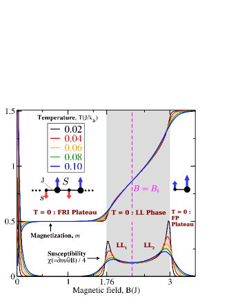
Figure 1: (color online). Magnetization plateaus at finite temperature, Luttinger liquid phase and crossovers: Quantum Monte Carlo (QMC) data. Magnetization per cell $m$ and the susceptibility $\chi=\partial m/\partial B$ as a function of magnetic field $B$ for an alternating ($s=1/2$, $S=1$) chain with $N=256$ unit cells and the indicated values of temperature $T$. The critical endpoint of the ferrimagnetic (FRI) and the fully polarized (FP) plateaus are $B_{c,FRI}=1.76J$ and $B_{c,FP}=3J$, respectively. The presence of the FRI and FP plateaus, and the region dominated by Luttinger liquid (LL) regime is a common feature for all values of $s$ and $S$, with $S>s$. As $T\rightarrow 0$, $\chi\rightarrow\infty$ at the critical values of $B$; for $T\gtrsim 0$, local maxima in the $\chi$ curves marks the crossover from the LL regime to the quantum critical regime. The local minimum in the $\chi$ curve (dashed line) between $B_{c,FRI}$ and $B_{c,FP}$ separates the LL regime into two regions: one with excitations from the FRI state, $\text{LL}_{1}$; the other with excitations from the FP state, $\text{LL}_{2}$.

In Fig. 1 we show QMC results for $m(B)$ for the (1/2, 1) chain in the low-$T$ regime. At $T=0$, $m(B)$ presents two magnetization plateaus: the ferrimagnetic (FRI), at $m_{FRI}=(S-s)$, and the fully polarized (FP) one, at $m_{FP}=s+S$. In particular, at $T=0$, $m=m_{FRI}$ for $B=0$, with a gapless Goldstone mode. There are quantum phase transitions at the endpoint of the plateaus: $B=B_{c,FRI}$ and $B=B_{c,FP}$, respectively; which have the values $B_{c,FRI}=1.76J$ and $B_{c,FP}=3.00J$ for the ($1/2$, $1$) chain. At the critical fields, there is a transition from a gapped plateau phase to a gapless Luttinger liquid (LL) phase, as $B\rightarrow B_{c,FRI}$ from magnetic fields $B<B_{c,FRI}$, or $B\rightarrow B_{c,FP}$ from magnetic fields $B>B_{c,FP}$. In the LL phase, the excitations have a linear dispersion relation, $\omega\sim q$, and present critical (power-law) transverse spin correlations. Exactly at the critical fields, the excitations have a classical dispersion relation $\omega\sim q^{2}$ and in the high diluted limit can be represented by a hard-core boson model or a spinless fermion model. Hence, the magnetization has a square-root behavior $m\sim\sqrt{|B-B_{c}|}$ and a diverging susceptibility $\chi=\partial m/\partial B\sim 1/\sqrt{|B-B_{c}|}$ as $B\rightarrow B_{c}$.

For finite-$T$, but $T\rightarrow 0$, the magnetization $m=0$ for $B=0$, since the system is one-dimensional. Gapped magnetic excitations are thermally activated and the plateau widths reduce. The susceptibility shows local maxima, with distinct amplitudes, at $B\approx B_{c,FRI}$ and $B\approx B_{c,FP}$ marking the crossover between the LL regime, where the excitations have a linear behavior, $\omega\sim q$, to the quantum critical regime, for which $\omega\sim q^{2}$. We can define the local minimum in the $\chi$ curve, at $B\equiv B_{i}$, as a crossover between the region where the excitations are predominantly from the FRI state, denoted by LL₁ in Fig. 1, and that where the excitations are predominantly from the FP state, denoted by LL₂ in Fig. 1. In particular, for $B\approx B_{i}$, the magnetization curve has its more robust value and behavior as the temperature increases, showing that the LL phase is more robust for $B\approx B_{i}$.

III Spin-wave Theory

The ferrimagnetic arrangement of classical spins is a natural choice of vacuum to study quantum ferrimagnets through free spin-wave (FSW) theory Pati et al. (1997a); *PhysRevB.55.8894, if we want to study excitations from the quantum ground state. Two types of magnon excitations are obtained, one ferromagnetic, which decreases the ground state spin by one unit, and the other antiferromagnetic, increasing the ground state spin by one unit. In particular, the antiferromagnetic excitation has a finite gap $\Delta$, which implies the expected magnetization plateau at $m=S-s$ and $T=0$. However, at this linear approximation, quantum fluctuations are underestimated, giving poor results for the value of antiferromagnetic gap, and other quantities, like the average spin per site.

When one-dimensional ferromagnets are studied through the linear spin-wave theory at finite temperatures, a diverging zero-field magnetization is obtained for any value of $T$Holstein and Primakoff (1940); Anderson (1952); Kubo (1952). Takahashi Takahashi (1986, 1987) modified the theory by imposing a constraint on the zero-field magnetization and an effective chemical potential in the thermal boson distribution. This so-called modified spin-wave theory describes very well the low-temperature thermodynamics of one-dimensional ferromagnets, and was further successfully adapted to other systems, including ferrimagnetic chains Yamamoto and Fukui (1998). In the case of ferrimagnets, the introduction of the magnetization constraint in the bosonic distribution, with the linear spin-wave dispersion relations gives an excellent description of the low-$T$ behavior. The description of the intermediate-$T$ regime can be improved by changing the constraint Noriki and Yamamoto (2017).

In this Section, we discuss interacting spin-wave theory using a ferrimagnetic vacuum (ISW-FRIv) for $B\neq 0$ and $T\neq 0$, with the modified spin-wave approach (Takahashi’s constraint); and free spin-wave theory from a fully polarized vacuum (FSW-FPv), also for $B\neq 0$ and $T\neq 0$.

III.1 Spin-wave theory - ferrimagnetic vacuum

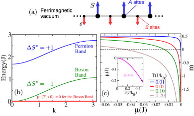
Figure 2: (color online). Interacting spin-wave (ISW) magnon branches from the classical ferrimagnetic vacuum (FRIv) - calculating the thermodynamic properties. (a) The classical ferrimagnetic vacuum of the ($s$,$S$) chain. (b) Magnon dispersion relations for the ($s=1/2$, $S=1$) chain with $B=0$. There are ferromagnetic and antiferromagnetic magnons, carrying spin $\Delta S^{z}=-1$ and $\Delta S^{z}=1$, respectively. The values of the critical fields are $B^{(\textsc{ISW-FRIv})}_{c,\textsl{FRI}}=1.68J$ and $B^{(\textsc{ISW-FRIv})}_{c,\textsl{FP}}=2.74J$. To calculate the thermodynamic functions, the antiferromagnetic (ferromagnetic) magnons occupies their respective bands following the Fermi (Bose) distribution function. An effective chemical potential $\mu$ is introduced in the Bose distribution to prevent particle condensation at the $k=0$ mode for $B=0$ and $T\rightarrow 0$. (c) For each value of $T$, we use a value of $\mu$ such that $m=0$ for $B=0$. The inset shows that $\mu(T\rightarrow 0)\rightarrow 0$ as $T\rightarrow 0$. In this limit, both bands are empty and $m=(S-s)=1/2$, the FRI magnetization.

The Holstein-Primakoff spin-wave theory is developed from the classical ground state illustrated in Fig. 2(a), which has the energy $E^{\text{\tiny{(FRIv)}}}_{class}=-2JNsS-B\big{(}S-s\big{)}N$. The bosonic operators $a_{j}$ ($a^{\dagger}_{j}$) and $b_{j}$ ($b^{\dagger}_{j}$), associated to $A$ and $B$ sites, respectively, have the following relation with the spin operators (Holstein-Primakoff transformation):

$$S^{+}_{j} = \sqrt{2S}\Big{(}1-\frac{a^{\dagger}_{j}a_{j}}{2S}\Big{)}^{1/2}a_{j}\text{, and }S^{z}_{j}=S-a^{\dagger}_{j}a_{j};$$ (3)

$$s^{+}_{j} = b^{\dagger}_{j}\sqrt{2s}\Big{(}1-\frac{b^{\dagger}_{j}b_{j}}{2s}\Big{)}^{1/2}\text{, and }s^{z}_{j}=b^{\dagger}_{j}b_{j}-s.$$ (4)

Putting the Hamiltonian (1) in terms of these bosonic operators, expanding to quadratic order, Fourier transforming and making the following Bogoliubov transformation Pati et al. (1997a); *PhysRevB.55.8894:

$$a_{k}=\alpha_{k}\cosh\theta_{k}-\beta_{k}^{\dagger}\sinh\theta_{k},$$

$$b_{k}=\beta_{k}\cosh\theta_{k}-\alpha_{k}^{\dagger}\sinh\theta_{k},$$ (5)

$$\tanh 2\theta_{k}=2\frac{\sqrt{sS}}{s+S}\cos\Big{(}\frac{k}{2}\Big{)},$$ (6)

where $k$ is the lattice wave-vector, the non-interacting spin-wave Hamiltonian is given by

$$\mathcal{H}^{\text{\tiny{(FSW-FRIv)}}}=E_{0}+\sum_{k}\Big{[}\omega^{\text{\tiny{(FRIv)}}}_{k,-}\alpha_{k}^{\dagger}\alpha_{k}+\omega^{\text{\tiny{(FRIv)}}}_{k,+}\beta_{k}^{\dagger}\beta_{k}\Big{]}.$$ (7)

The magnon branches obtained are:

$$\omega^{\text{\tiny{(FRIv)}}}_{k,\sigma}=\sigma J\big{(}S-s\big{)}-\sigma B+J\omega^{\text{\tiny{(FRIv)}}}_{k},$$ (8)

with $\sigma=\pm$, and

$$\omega^{\text{\tiny{(FRIv)}}}_{k}=\sqrt{\big{(}S-s\big{)}^{2}+4sS{\sin}^{2}\Big{(}\frac{k}{2}\Big{)}},$$ (9)

while the ground-state energy is

$$E_{0}=J\sum_{k}\Big{[}\omega^{\text{\tiny{(FRIv)}}}_{k}-\big{(}S+s\big{)}\Big{]}.$$ (10)

The $\omega^{\text{\tiny{(FRIv)}}}_{k,-}$ modes carry a spin $\Delta S^{z}=-1$, having a ferromagnetic spin-wave nature, and is gapless for $B=0$; while $\omega^{\text{\tiny{(FRIv)}}}_{k,+}$ modes carry a spin $\Delta S^{z}=+1$, having an antiferromagnetic spin-wave nature and has a gap $\Delta=2J(S-s)$ at $B=0$. For the ($s=1/2$, $S=1$) chain Pati et al. (1997a); *PhysRevB.55.8894, for example, $\Delta=1$, although the exact value is $1.76J$; while $\langle S^{z}_{a}\rangle=0.695$ and $\langle S^{z}_{b}\rangle=-0.195$ at $T=0$, with the exact values Pati et al. (1997a); *PhysRevB.55.8894: $\langle S^{z}_{a}\rangle=0.792$ and $\langle S^{z}_{b}\rangle=-0.292$.

The dispersion relations can be improved if interactions between magnons are considered. The corrected dispersion relations described in Ref. Yamamoto et al. (1998b), shown in Fig. 2(b), are:

$$\tilde{\omega}^{\text{\tiny{(FRIv)}}}_{k,\sigma}={\omega}^{\text{\tiny{(FRIv)}}}_{k,\sigma}-J\delta{\omega}^{\text{\tiny{(FRIv)}}}_{k,\sigma},$$ (11)

where

$$\delta\omega^{\text{\tiny{(FRIv)}}}_{k,\sigma}=2\Gamma_{1}\frac{(S+s)}{\omega^{\text{\tiny{(FRIv)}}}_{k}}\sin^{2}(k/2)-\frac{\Gamma_{2}}{\sqrt{sS}}\Big{[}\omega^{\text{\tiny{(FRIv)}}}_{k}+\sigma(S-s)\Big{]},$$

with

$$\Gamma_{1} = \frac{1}{N}\sum_{k}\sinh^{2}\theta_{k},\text{ and}$$ (12)

$$\Gamma_{2} = \frac{1}{N}\sum_{k}\cos(k/2)\sinh\theta_{k}\cosh\theta_{k}.$$ (13)

Up to $\mathcal{O}(S^{0})$, the Hamiltonian is

$$\mathcal{H}^{\text{\tiny{(ISW-FRIv)}}}=E_{g}+\sum_{k}\big{(}\tilde{\omega}^{\text{\tiny{(FRIv)}}}_{k,-}\alpha^{{\dagger}}_{k}\alpha_{k}+\tilde{\omega}^{\text{\tiny{(FRIv)}}}_{k,+}\beta^{{\dagger}}_{k}\beta_{k}\big{)},$$ (14)

where

$$E_{g}=E_{class}+E_{0}+E_{1},$$ (15)

with

$$E_{1}=-2JN\Big{[}\Gamma_{1}^{2}+\Gamma_{2}^{2}-\Big{(}\sqrt{S/s}+\sqrt{s/S}\Big{)}\Gamma_{1}\Gamma_{2}\Big{]}.$$ (16)

At $T=0$, the magnetization as a function of $B$, shown in Fig. 1 for the ($s=1/2$, $S=1$) chain, can be understood from these ferromagnetic ($\Delta S^{z}=-1$) and antiferromagnetic ($\Delta S^{z}=+1$) magnon modes. For $B=0$ the two bands are empty and the magnetization is the ferrimagnetic one. Increasing the magnetic field, the ferromagnetic band acquires a gap which increases linearly with $B$, while the gap to the antiferromagnetic band decreases linearly with $B$. Notice, in particular, that the ferromagnetic band is empty for all values of $B$. At $B=B^{(\textsc{ISW-FRIv})}_{c,\textsl{FRI}}/2=\Delta/2$, the $k=0$ mode of the antiferromagnetic band is the lower energy state, and at $B=B^{(\textsc{ISW-FRIv})}_{c,\textsl{FRI}}=\Delta$ the gap to this mode closes. The value of $B^{(\textsc{ISW-FRIv})}_{c,\textsl{FRI}}$ is

$$B^{(\textsc{ISW-FRIv})}_{c,\textsl{FRI}}=\tilde{\omega}^{\text{\tiny{(FRIv)}}}_{0,+}=2(S-s)\left(1+\frac{1}{\sqrt{sS}}\Gamma_{2}\right)J.$$ (17)

In particular, for the ($s=1/2$, $S=1$) chain, with $\Gamma_{1}=0.305$ and $\Gamma_{2}=0.478$, $B^{(\textsc{ISW-FRIv})}_{c,\textsl{FRI}}=1.68J$, which is very close to the exact value ($1.76J$).

The magnetization for $B>\Delta$ is obtained by considering the antiferromagnetic magnons as hard-core bosons Affleck (1991), or spinless fermions. The magnetization increases with $B$ as the antiferromagnetic band is filled, and saturates when the Fermi level reaches the band limit, at $k=\pi$. The saturation field is

$$B^{(\textsc{ISW-FRIv})}_{c,\textsl{FP}}=\tilde{\omega}^{\text{\tiny{(FRIv)}}}_{\pi,+}=2\left(S-\Gamma_{1}+\sqrt{\frac{S}{s}}\Gamma_{2}\right)J,$$ (18)

which for the ($s=1/2$, $S=1$) chain is $B^{(\textsc{ISW-FRIv})}_{c,\textsl{FP}}=2.74$, departing from the exact value $3J$, but much better than the free spin wave result: $2J$.

III.1.1 Thermodynamics

For $T>0$, ferromagnetic and antiferromagnetic modes are occupied in accord to Bose-Einstein ($n^{\text{\tiny{(FRIv)}}}_{k,-}$) and Fermi-Dirac ($n^{\text{\tiny{(FRIv)}}}_{k,+}$) distributions, respectively, as indicated in Fig. 2(a). The magnetization, for example, is given by

$$m(T,B)=(S-s)+\frac{1}{N}\sum_{k}(n^{\text{\tiny{(FRIv)}}}_{k,+}-n^{\text{\tiny{(FRIv)}}}_{k,-}).$$ (19)

We notice, however, that with $T>0$ and $B=0$ the ferromagnetic band will be thermally activated and $m\rightarrow-\infty$ as $T$ increases. This problem arises, also, in one-dimensional ferromagnetic chains, and was overcome by Takahashi Takahashi (1986, 1989), in the low-$T$ regime, through the introduction of an effective chemical potential $\mu$ in the bosonic distribution, and a constraint $m(B=0,T)=0$. A similar strategy was applied to one-dimensional ferrimagnetic systems Yamamoto and Fukui (1998) and good results were also obtained in the low-$T$ regime. The intermediate-$T$ regime, where the minimum in the $T\chi$ curve of the ferrimagnets Verdaguer et al. (1984) are observed, can be more accurately described if other constraints are used Yamamoto (2004); Yamamoto et al. (1998b); Noriki and Yamamoto (2017).

Here, for $B=0$, we use the simplest constraint

$$m(T,B=0)=0,$$ (20)

since we are interested in the low-$T$ regime, with

$$n^{\text{\tiny{(FRIv)}}}_{k,-} = \frac{1}{e^{\beta[\tilde{\omega}^{\text{\tiny{(FRIv)}}}_{k,-}-\mu]}-1},$$ (21)

$$n^{\text{\tiny{(FRIv)}}}_{k,+} = \frac{1}{e^{\beta\tilde{\omega}^{\text{\tiny{(FRIv)}}}_{k,+}}+1}.$$ (22)

In Fig. 2(b), we present $m(T,B=0)$ for the indicated values of $T$. As discussed, $m\rightarrow-\infty$ at $\mu=0$ and the value of $\mu$ for which the constraint $m(T,B=0)=0$ is satisfied, monotonically decreases with $T$, in this low-$T$ regime. A finite $\mu$ implies an effective gap for the ferromagnetic band, with an exponential thermal activation of their magnons. In particular, notice that $\mu(T\rightarrow 0)=0$, as expected. To calculate the thermodynamic functions for $B\neq 0$, we consider the distributions in Eqs. (21) and (22) and use the same value of $\mu$ found in the case $B=0$: $\mu(B,T)=\mu(B=0,T)$, for any value of $B$.

The magnetization as a function of $B$ for $T\neq 0$, shown in Fig. 1, can be qualitatively understood from this theory. For $B=0$, the magnetization $m=0$, due to the constraint. As $B$ increases, in the region $0<B<B_{c,FRI}/2$, the gap to the ferromagnetic band increases, but this band is thermally activated and the magnetization decreases from the $m=S-s$ value. This effect can also be seen from Fig. 2(b). If we move the Zeeman term, $+B$, from the ferromagnetic dispersion relation to the chemical potential, $\tilde{\omega}^{\text{\tiny{(FRIv)}}}_{k,-}\rightarrow\tilde{\omega}^{\text{\tiny{(FRIv)}}}_{k,-}-B$ and $-\mu\rightarrow-(\mu-B)$, in Eq. (21), the magnetization value is the one shown in Fig. 2(b) for $\mu$ lower than that of $B=0$, and $m=0$. From Fig. 2(b), we see that increasing $B$ (decreasing $\mu$) from $B=0$ [from $\mu(B=0,T)$], the magnetization rises exponentially to the ferrimagnetic value. For $B=B^{(\textit{\tiny{FSW, FPv}})}_{c,FRI}/2$, the lower energy band is the antiferromagnetic ($\Delta S^{z}=+1$ magnons) fermionic band. This band is thermally activated for $[B^{(\textit{\tiny{FSW, FPv}})}_{c,FRI}/2]<B<B_{c,FRI}$, and the magnetization is higher than $S-s$. The magnetization increases through the filling of this band, in accord to the Fermi distribution, up to the saturation value $m=s+S$, which is exponentially reached.

III.2 Spin-wave theory - fully polarized vacuum

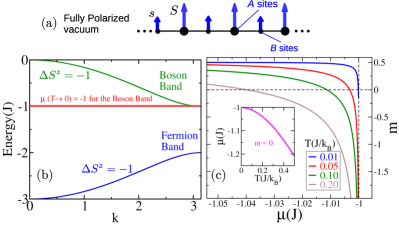
Figure 3: (color online). Free spin-wave magnon branches from the classical ferromagnetic vacuum - calculating the thermodynamic properties. (a) The classical fully polarized vacuum of the ($s$,$S$) chain. (b) Free spin-wave (FSW) results for the magnon energies relative to the fully polarized vacuum (FPv) for $T\neq 0$ and $B=0$ for the ($s=1/2$, $S=1$) chain. In this case, both branches are ferromagnetic with magnons carrying a spin $\Delta S^{z}=-1$. To calculate the thermodynamic functions, the lower (higher) magnon band is filled following the Fermi (Bose) distribution function. An effective chemical potential $\mu$ is introduced in the Bose distribution to prevent particle condensation at the $k=\pi$ mode for $B=0$ and $T\rightarrow 0$. The critical fields are $B^{(\textit{\tiny{FSW, FPv}})}_{c,FRI}=2.00J$ and $B^{(\textit{\tiny{FSW, FPv}})}_{c,FP}=3.00J$. (c) The chemical potential $\mu$ is chosen such that $m=0$ for $B=0$. The inset shows that $\mu(T\rightarrow 0)\rightarrow-1$ as $T\rightarrow 0$. In this limit only the lower energy band is occupied, implying that $m\rightarrow(S-s)=1/2$, the ferrimagnetic magnetization, as $T\rightarrow 0$ and $B\rightarrow 0$.

In this section, we study the free spin wave theory from a fully polarized vacuum, illustrated in Fig. 3(a). We show that this theory provides a good description of the low-$T$ physics, and is quantitatively much better than the free spin wave description from the ferrimagnetic vacuum. The critical saturation field has an exact value, while the critical field at the end of the ferrimagnetic plateau is $B^{(\textit{\tiny{FSW, FPv}})}_{c,FRI}=2J$.

The Holstein-Primakoff transformation in this case is

$$S^{+}_{j} = \sqrt{2S}\Big{(}1-\frac{a^{\dagger}_{j}a_{j}}{2S}\Big{)}^{1/2}a_{j}\text{, and }S^{z}_{j}=S-a^{\dagger}_{j}a_{j};$$ (23)

$$s^{+}_{j} = \sqrt{2s}\Big{(}1-\frac{b^{\dagger}_{j}b_{j}}{2s}\Big{)}^{1/2}b_{j}\text{, and }s^{z}_{j}=s-b^{\dagger}_{j}b_{j},$$ (24)

with the two bosons lowering the site magnetization by one unit. To quadratic order in these bosonic operators, the Hamiltonian of the system, Eq. (1), is

$$\mathcal{H}^{\text{\tiny{(FSW-FPv)}}} = E^{\text{\tiny{(FPv)}}}_{class}+J\sum_{j}\Bigg{\{}-s\Big{(}a_{j}^{\dagger}a_{j}+a_{j+1}^{\dagger}a_{j+1}\Big{)}$$ (25)

$$- 2Sb_{j}^{\dagger}b_{j}+\sqrt{sS}\Bigg{[}\Big{(}a_{j}+a_{j+1}\Big{)}b_{j}^{\dagger}+\Big{(}a_{j}^{\dagger}+a_{j+1}^{\dagger}\Big{)}b_{j}\Bigg{]}$$

$$+ B\sum_{j}\Big{(}a_{j}^{\dagger}a_{j}+b_{j}^{\dagger}b_{j}\Big{)}\Bigg{\}},$$

with $E^{\text{\tiny{(FPv)}}}_{class}=2JNsS-B\big{(}S+s\big{)}N$. Fourier transforming the bosonic operators and using the Bogoliubov transformation

$$a_{k}^{\dagger} = \alpha_{k}^{\dagger}\cos\theta_{k}-\beta_{k}^{\dagger}\sin\theta_{k};$$ (26)

$$b_{k}^{\dagger} = \beta_{k}^{\dagger}\cos\theta_{k}+\alpha_{k}^{\dagger}\sin\theta_{k},$$ (27)

with

$$\tan 2\theta_{k}=2\frac{\sqrt{sS}}{S-s}\cos\Big{(}\frac{k}{2}\Big{)},$$ (28)

the Hamiltonian in Eq. 25 is written as

$$\mathcal{H}^{\text{\tiny{(FSW-FPv)}}}=E^{\text{\tiny{(FPv)}}}_{class}+\sum_{k}\Big{[}\omega^{\text{\tiny{(FPv)}}}_{k,1}\alpha_{k}^{\dagger}\alpha_{k}+\omega^{\text{\tiny{(FPv)}}}_{k,0}\beta_{k}^{\dagger}\beta_{k}\Big{]},$$ (29)

where the dispersion relations Maisinger et al. (1998) $\omega^{\text{\tiny{(FPv)}}}_{k,\eta}$ are

$$\omega^{\text{\tiny{(FPv)}}}_{k,\eta} = (-1)^{\eta+1}\sqrt{\big{(}S-s\big{)}^{2}+4sS{\cos}^{2}\Big{(}\frac{k}{2}\Big{)}}$$ (30)

$$-\big{(}S+s\big{)}+B,$$

with $\eta=0\text{ or }1$.

To discuss the $T=0$ magnetization curve implied by these spin-wave modes, we present in Fig. 3(b) the dispersion relations $\omega^{\text{\tiny{(FPv)}}}_{k,\eta}$ for the ($s=1/2$, $S=1$) chain and $B=B^{(\textit{\tiny{FSW, FPv}})}_{c,FP}=2J(s+S)=3J$. At $B=B^{(\textit{\tiny{FSW, FPv}})}_{c,FP}=B_{c,FP}$, both bands are empty, and the magnetization is the fully polarized one. Decreasing $B$, the $\eta=0$ band is filled in accord to Fermi-Dirac statistics, and the magnetization decreases. The critical field at the end point of the ferrimagnetic plateau is obtained making $\omega^{\text{\tiny{(FPv)}}}_{\pi,0}=0$, which implies $B^{(\textit{\tiny{FSW, FPv}})}_{c,FRI}=2SJ$, equal to $2J$ for the ($s=1/2$, $S=1$) chain. At this value of $B$, the $\eta=0$ band is totally filled and $m=(s+S)-1$, giving $1/2$ for the ($s=1/2$, $S=1$) chain. There is a gap of $2(S-s)J$ between the $\eta=0$ and $\eta=1$ bands, at $k=\pi$; hence, the bosonic $\eta=1$ band should start to be filled at $B=B^{(\textit{\tiny{FSW, FPv}})}_{c,FRI}-2(S-s)J$, and the theory does not qualitatively reproduce the $T\rightarrow 0$ magnetization curve. This problem is overcome by considering the finite temperature theory, with Takahashi’s constraint and effective chemical potential. For finite $T$, the magnetization is given by

$$m(T,B)=(S+s)-\frac{1}{N}\sum_{k}[n^{\text{\tiny{(FPv)}}}_{k,0}+n^{\text{\tiny{(FPv)}}}_{k,1}],$$ (31)

where

$$n^{\text{\tiny{(FPv)}}}_{k,0} = \frac{1}{e^{\beta\omega^{\text{\tiny{(FPv)}}}_{k,0}}+1},$$ (32)

$$n^{\text{\tiny{(FPv)}}}_{k,1} = \frac{1}{e^{\beta[\omega^{\text{\tiny{(FPv)}}}_{k,1}-\mu]}-1}.$$ (33)

The constraint, which is applied at $B=0$, is

$$m(T,B=0)=0.$$ (34)

In Fig. 3(c) we present the magnetization as a function of the effective chemical $\mu$ for the indicated values of temperature. We note that $m\rightarrow-\infty$ as the temperature increases, similarly to the spin-wave theory with the ferrimagnetic vacuum. However, in this case $\mu\rightarrow-1$ as $T\rightarrow 0$, as shown in Fig. 3(b). Hence, a finite chemical potential $\mu=-1$ associated to the bosonic $\eta=1$ band must be considered in the $T=0$ theory. With this chemical potential, the $\eta=1$ band stays empty at $T=0$ for any value of $B$.

The thermodynamic functions are calculated using Eq. 33, with $\mu(T,B)=\mu(T,B=0)$. For finite $T$, the fermionic $\eta=0$ band is completely filled and the occupation of the $\eta=1$ band is such that $m=0$. Considering the low-$T$ regime, as $B$ increases, the energy of the two bands raises, lowering the total occupation of the $\eta=1$ band, since $\omega^{\text{\tiny{(FPv)}}}_{k,1}-\mu$ linearly increases with $B$ for any $k$, and $m$ increases. The magnetization exponentially reaches its value at the ferrimagnetic plateau, $m=S-s$, as $B$ increases, since $n^{\text{\tiny{(FPv)}}}_{k,1}\rightarrow 0$ for any $k$ and the $\eta=0$ band is completely filled. For $[B^{(\textit{\tiny{FSW, FPv}})}_{c,FRI}/2]<B<B^{(\textit{\tiny{FSW, FPv}})}_{c,FRI}$, with $[B^{(\textit{\tiny{FSW, FPv}})}_{c,FRI}/2]$ related to the point $B=B_{c,FRI}/2$ in Fig. 1, the occupation of the $\eta=0$ band decreases from the $T=0$ case: $n^{\text{\tiny{(FPv)}}}_{k,0}=1$ for any $k$, and the magnetization is higher than $S-s$. The magnetization increases with $B$, and exponentially reaches the fully polarized value at $B>B^{(\textit{\tiny{FSW, FPv}})}_{c,FP}$, since magnons at the $\eta=0$ band are thermally excited.

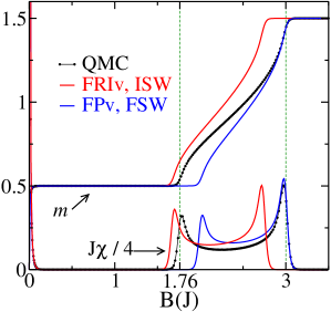
Figure 4: (color online). Comparison between results from quantum Monte Carlo (QMC) method, $N=256$ unit cells, and the two spin-wave approaches for the magnetization per cell $m$ and the susceptibility $\chi$: ($s=1/2$, $S=1$) chain at temperature $T=0.02(J/k_{B})$. Results from the interacting spin-wave theory from a ferrimagnetic vacuum (ISW-FRIv) and free spin-wave theory from a ferromagnetic vacuum (FSW-FPv) compare well with QMC for $B\lesssim B_{c,FRI}$ and $B\gtrsim B_{c,FP}$. The maximum in $\chi$ related to $B_{c,FRI}$ ($B_{c,FP}$) is better localized, compared to QMC, through the ISW-FRIv (FSW-FPv) approach.

III.3 Comparison between QMC data and the two spin-wave approaches

In Fig. 4 we present magnetization and susceptibility $\chi=\partial m/\partial B$ as a function of $B$ from ISW-FRIv and FSW-FPv theories along with QMC data, at $T=0.1J$. Since the ISW-FRIv gives a better result for $B_{c,FRI}$, this theory is better in the vicinity of this critical field. Otherwise, the FSW-FPv approach is better in the vicinity of $B_{c,FP}$. Further, the amplitudes of the two peaks in $\chi(B)$, which marks the crossover to the LL regime, have values lower than the ones given by QMC. The difference between the amplitudes of the spin-wave approaches and QMC data is related to limitations in the spin-wave theories. Despite it, the description from both spin-wave theories are qualitatively excellent, and quantitatively very acceptable in the low-$T$ regime.

Below we calculate the $T$ vs $B$ phase diagram in the low-$T$ regime from the FSW-FPv theory. We study the crossover lines between the LL regimes and the quantum critical regimes; as well as the crossovers lines between the plateau regimes and the quantum critical regimes. We use the FSW-FPv approach since it has essentially the same precision of the ISW-FRIv theory, if we consider a range of $B$ from 0 to the saturation field; also, the critical point $B_{c,FP}$ is exact in the FSW-FPv theory.

IV Luttinger liquid regime

In the LL phase, the dispersion relation can be approximated by $\pm v_{F}|k-k_{F}|$, where $v_{F}$ is the Fermi velocity. Further, in this regime the magnetization has the form Maeda et al. (2007):

$$m=m(T=0)-\frac{\pi}{6v_{F}^{2}}\frac{\partial v_{F}}{\partial B}(k_{B}T)^{2}+O(T^{3}).$$ (35)

In our case, the Fermi velocity along the $\eta=0$ band is $v_{F}=[\partial\omega^{\text{\tiny{(FPv)}}}_{k,0}/\partial k]_{k=k_{F}}$, with $k_{F}$ calculated from $\omega^{\text{\tiny{(FPv)}}}_{k,0}|_{k=k_{F}}=0$.

In Fig. 5(a) we present $v_{F}$ as a function of $B$ for the (1/2,1) chain. Near the critical fields, $|\partial v_{F}/\partial B|$ is large and $v_{F}$ little. For a fixed $B\gtrsim B^{(\textit{\tiny{FSW, FPv}})}_{c,FRI}$, as shown in Fig. 5(b), the magnetization presents a fast decay from the $T=0$ value as $T$ increases. Also, for $B\lesssim B^{(\textit{\tiny{FSW, FPv}})}_{c,FP}$, as shown in Figs. 5(c), $m$ increases from $m(0)$. In both cases, the curvature of the $m(T\rightarrow 0)$-curve increases as $B$ get closer to the critical fields. The crossover temperature $T(B)$ of the LL regime at a fixed $B$ is defined as the point at which $m(T)$ departs from the quadratic behavior in Eq. (35). So, $T(B)$ is taken to be at the minima ($B\gtrsim B^{(\textit{\tiny{FSW, FPv}})}_{c,FRI}$) and maxima ($B\lesssim B^{(\textit{\tiny{FSW, FPv}})}_{c,FP}$) of the $m(T)$ curve Maeda et al. (2007). In particular, as $B\rightarrow B_{c}$ the crossover line separates the LL regime and the quantum critical regime, for which the excitations have a quadratic dispersion relation. In this case, a universal, model independent, straight line $k_{B}T(B)=a|B-B_{c}|$, with $a=0.76238$, can be derived Maeda et al. (2007).

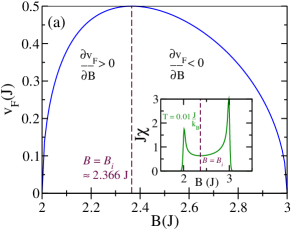
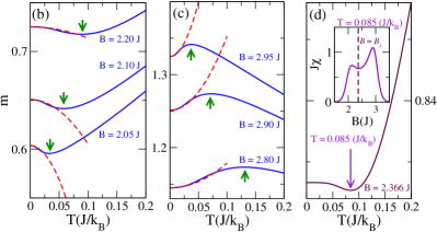
Figure 5: (color online). Results from the free spin-wave approach with the fully polarized vacuum (FSW-FPv). (a) Fermi velocity $v_{F}$ as a function of the magnetic field $B$ and [(b), (c) and (d)] magnetization curves $m(T)$. (a) $\partial v_{F}/\partial B\rightarrow+\infty$ and $v_{F}\rightarrow 0$ as $B\rightarrow B^{(\textit{\tiny{FSW, FPv}})}_{c,FRI}=2.00J$, while $\partial v_{F}/\partial B\rightarrow-\infty$ and $v_{F}\rightarrow 0$ as $B\rightarrow B^{(\textit{\tiny{FSW, FPv}})}_{c,FP}=3.00J$. As shown in the inset, for $B=B_{i}\approx 2.366J$, $\partial v_{F}/\partial B=0$ and the susceptibility $\chi(B)$ has a minimum at this value of $B$. (b) $m(T)$ for the indicated values of $B$ in the vicinity of the critical field $B^{(\textit{\tiny{FSW, FPv}})}_{c,FRI}$. (c) $m(T)$ for values of $B$ in the vicinity of the critical field $B^{(\textit{\tiny{FSW, FPv}})}_{c,FP}$. (d) $m(T)$ for $B=B_{i}$. The $m(T)$ curves to order $O(T^{2})$, Eq. (35), are shown as dashed lines in (b) and (c) for the corresponding values of $B$, arrows indicate local extreme points in $m(T)$, which are used as a criterium to identify the LL regime. The inset in (d) shows that the minimum in $m(T)$ is associated to the local minimum in $\chi(B)$, which is found between the two critical fields.

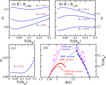
Figure 6: (color online). Magnetization per cell $m(T)$ with fixed $B$: calculating the crossover lines bounding the Luttinger liquid regime. Quantum Monte Carlo (QMC) results for the magnetization curves $m(T)$ and the crossover lines for a system with $N=128$. (a) $m(T)$ for values of $B$ in the vicinity of the critical field $B_{c,FRI}=1.76J$. (b) $m(T)$ for values of $B$ in the vicinity of the critical field $B_{c,FP}=3.00J$. (c) $m(T)$ for a value of $B$ such that $\partial\chi/\partial B\approx 0$ at $T=0$ and inside the Luttinger liquid phase, dashed line in Fig. 1. (d) Local extreme points of $m(T)$ curves from QMC and free spin-wave from the fully polarized vacuum (FSW-FPv). In the case of the FSW-FPv local minima, we shift $B$ by $B_{c,FRI}-B^{(\textit{\tiny{FSW, FPv}})}_{c,FRI}\approx 0.24J$. The exact crossover straight lines as $T\rightarrow 0$, extended in the figure for better visualization: $a|B-B_{c,FRI}|$ and $a|B-B_{c,FP}|$, with $a=0.76238$, are also shown. The error bars are defined as half the temperature step ($\Delta T=0.008$) used to calculate $m(T)$.

In the inset of Fig. 5(a), we show that the minimum in the $\chi(B)=\partial m/\partial B$ curve is found at $B=B_{i}$, a value of $B$ at which $|\partial v_{F}/\partial B|=0$. This value of $B$ marks a crossover from the regime where excitations are predominantly from the FRI critical state to the regime where they come from the FP critical state. At $B=B_{i}$, the Fermi wave-vector is at the inflection point of the dispersion curve ($d^{2}\omega^{\text{\tiny{(FPv)}}}_{k,0}/dk^{2}=0$), since

$$\frac{\partial v_{F}}{\partial B}=\left[\frac{d^{2}\omega^{\text{\tiny{(FPv)}}}_{k,0}}{dk^{2}}\right]_{k=k_{F}}\left(\frac{\partial k_{F}}{\partial B}\right),$$ (36)

and $k_{F}$ increases monotonically with $B$ between the critical fields. If the value of $k$ at the inflection point is $k_{i}$, we can calculate $B_{i}$ from the equation $\omega^{\text{\tiny{(FPv)}}}_{k_{i},0}=0$. For the (1/2,1) chain, for example, $B_{i}=2.366J$ and is indicated in Fig. 5(a).

At $B=B_{i}$, $\partial v_{F}/\partial B=0$ and the quadratic term in Eq. (35) is absent. So, the more stable, against $T$, LL region is found for $B\approx B_{i}$. Since the crossover temperatures $T(B)\rightarrow 0$ near the critical fields, the $T(B)$ line has an asymmetric dome-like profile, which is a consequence of the $v_{F}$ curve, shown in Fig. 5(a) for the case of the (1/2,1) chain, and is also observed in other quantum magnets Zapf et al. (2014).

A minimum in the $m(T)$ curve is also observed for $B=B_{i}$, due to the $O(T^{3})$ in Eq. (35), as shown in Fig. 5(d). In this case, however, this extreme point is associated with the minimum in the $\chi(B)$ curve, at $B=B_{i}$, as shown in the inset of Fig. 5(d).

In Fig. 6 we show $m(T)$ curves for the (1/2,1) chain calculated with QMC method to discuss the qualitatively agreement between these almost exact results and the conclusions from the spin-wave theory. In Figs. 6(a) and (b), we show the minimum (maximum) in the $m(T)$ curve for $B\gtrsim B_{c,FRI}=1.76J$ ($B\lesssim B_{c,FP}=3J$). In Fig. 6(c), we calculate $m(T)$ for a value of $B$ in the vicinity of the minimum in the $\chi(B)$ curve, $B=B_{i}$. Using the data in Fig. 1, it is located at $B_{i}=(2.27\pm 0.07)J$, and is indicated as a dashed line in that figure. As shown in Fig. 6(c), the $m(T\rightarrow 0)$ curve is also flat, as in Fig. 5(d), for $B=2.25J$. The minimum in the $m(T)$ curve appears at $T\approx 0.1J$. As can be observed in the $T=0.1J$ susceptibility curve in Fig. 1, it is also associated with the minimum in the $\chi(B)$ curve, at $B\approx B_{i}$.

In Fig. 6(d), we compare the position of the local extreme points in the $m(T)$ curves from QMC and FSW-FPv methods. The values of $B$ at the minima of $m(T)$ were translated by $B_{c,FRI}-B^{(\textit{\tiny{FSW, FPv}})}_{c,FRI}\approx 0.24J$. The lines for the maxima in $m(T)$ from both methods are in very good agreement since the FSW-FPv is almost exact for $T\rightarrow 0$, due to the low density of excited magnons in this temperature regime. Otherwise, the minima from both methods do not compare well, except for $T\rightarrow 0$, which is dominated by the critical point.

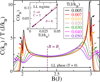
Figure 7: (color online). Specific heat from the free spin-wave theory from a fully polarized vacuum (FSW-FPv) for $T\rightarrow 0$. In the Luttinger liquid (LL) regime, $C\sim T$ as $T\rightarrow 0$, and $C/T$ is approximately constant for $B\approx B_{i}=2.366J$. The inset shows this linear behavior of $C$ at $B=B_{i}$. The crossover from the $T=0$ insulating plateau regime to the gapless quantum critical regime, at local maxima, are indicated by arrows.

We determine the crossover lines between the LL and plateau regimes through specific heat data, $C(B)$. In Fig. 7 we present FSW-FPv results for $C(B)$ in the low-$T$ regime. In the LL phase, at $T=0$, the specific heat $C\sim T$ as $T\rightarrow 0$, and $C/T$ is approximately constant in the LL regime, as shown in Fig. 7. The range of $B$ near $B=B_{i}$ is the more robust for this regime, and we present in the inset of Fig. 7 the linear behavior of $C$ as a function of $T$. For $B\lesssim B^{(\textit{\tiny{FSW, FPv}})}_{c,FRI}$ or $B\gtrsim B^{(\textit{\tiny{FSW, FPv}})}_{c,FP}$, the excitations are exponentially activated and the crossover to the quantum critical regime is marked by a local maximum in $C(B)$. The points of these crossover lines, $T_{\text{plateau}}(B)\sim|B-B_{c}|$, are indicated by arrows in Fig. 7. The quantum critical regime is bounded by this crossover line and that of the LL regime, which points appears as a second local maximum near $B^{(\textit{\tiny{FSW, FPv}})}_{c,FRI}$ and $B^{(\textit{\tiny{FSW, FPv}})}_{c,FP}$ in Fig. 7.

V Summary and discussions

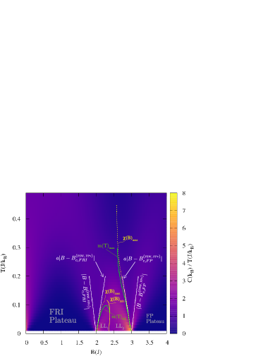
Figure 8: (color online). Spin-wave $T-B$ phase diagram of the ($s=1/2$, $S=1$) chain from the FPv. The quantum critical points $B^{(\textit{\tiny{FSW, FPv}})}_{c,FRI}=2.00J$ and $B^{(\textit{\tiny{FSW, FPv}})}_{c,FP}=3.00J$ bound the FRI and FP plateau regions, respectively. Increasing temperature, the plateau width decreases and the lines $k_{B}T=|B-B^{(\textit{\tiny{FSW, FPv}})}_{c,FRI}|$ and $k_{B}T=|B-B^{(\textit{\tiny{FSW, FPv}})}_{c,FP}|$ limit the plateau regions for $B\lesssim B_{c}$ [ferrimagnetic (FRI) plateau] and $B\gtrsim B_{c}$ [fully polarized (FP) plateau]. The LL regime has crossover lines given by $a|B-B^{(\textit{\tiny{FSW, FPv}})}_{c,FRI}|$ and $a|B-B^{(\textit{\tiny{FSW, FPv}})}_{c,FP}|$, with $a=0.76238$, for $B\rightarrow B_{c}$, as indicated by local maxima of the susceptibility $\chi(B)=\frac{\partial m}{\partial B}$, $\chi(B)_{max}$. Between these local maxima, there is a local minimum [$\chi(B)_{min}$] separating the regions under the influence of the $B^{(\textit{\tiny{FSW, FPv}})}_{c,FRI}$ critical point and that of the $B^{(\textit{\tiny{FSW, FPv}})}_{c,FP}$ one.

We have calculated the critical properties of alternating ferrimagnetic chains in the presence of a magnetic field from two spin-wave theories. We determine the better low-energy description of the excitations, considering the level of approximation, comparing the results with quantum Monte Carlo data. These ferrimagnetic chains present two magnetization ($m$) plateaus, the ferrimagnetic (FRI) plateau, for which $m=S-s$ and the fully polarized (FP) one, at $m=s+S$. The first spin-wave theory, is an interacting spin-wave (ISW) approach with the FRI classical vacuum, ISW-FRIv. The second methodology, is a free spin-wave (FSW) calculation from the FP state, FSW-FPv. In both cases, two bands are obtained. To calculate the finite temperature ($T$) properties of the system, one of the bands is considered as a bosonic band, with an effective chemical potential to prevent boson condensation at $B=0$; while the other is considered as a hard-core boson band, with a fermionic one-particle thermal distribution. Near the endpoint of the FRI plateau, the ISW-FRIv theory is a better option; while the FSW-FPv is exact for $T\rightarrow 0$ near the endpoint of the FP plateau. Since we are interested in describing the whole $T$ vs. $B$ phase diagram of the system, we deepen the study on the FSW-FPv, calculating the finite $T$ crossover lines bounding the plateau and the Luttinger liquid (LL) regimes.

In Fig. 8 we summarize our results in a $T$ vs. $B$ phase diagram, and show specific heat data $C/T$ as a function of $B$ and $T$. In the FRI and FP plateau regions the excitations are gapped, and $(C/T)\rightarrow 0$ as $T\rightarrow 0$. The gaps close at the quantum critical (QC) fields $B^{(\textit{\tiny{FSW, FPv}})}_{c,FRI}=2J$ and $B^{(\textit{\tiny{FSW, FPv}})}_{c,FP}=3J$, and local maxima appears in the values of $C/T$ for a fixed $T$. These local maxima indicate the crossover between the plateau and the QC regimes, and between the QC and LL regimes. As $T\rightarrow 0$, the crossover line between the plateau and the QC regimes (P-QC line) is a straight line $k_{B}T(B)=|B-B_{c}|$, for $B_{c}=B^{(\textit{\tiny{FSW, FPv}})}_{c,FRI}$ and $B_{c}=B^{(\textit{\tiny{FSW, FPv}})}_{c,FP}$; while a straight line $a|B-B_{c}|$, with a model-independent constant $a=0.76238$, marks the crossover between LL and QC regimes (LL-QC lines). The LL-QC line which contains the critical point $B=B^{(\textit{\tiny{FSW, FPv}})}_{c,FRI}$ $[B=B^{(\textit{\tiny{FSW, FPv}})}_{c,FP}]$ was also calculated from local minima (local maxima) in the $m(T)$ curves: $m(T)_{min}$ $[m(T)_{max}]$. The LL-QC lines were also calculated from local maxima in the susceptibility curve $\chi(B)$ at fixed $T$: $\chi_{max}(B)$.

The Luttinger liquid regime can be divided into two regions, separated by the minimum in the $\chi(B)$ curve with a fixed temperature, $\chi_{min}(B)$. The value of the magnetic field at which this minimum occurs at $T=0$, $B_{i}$, is at the inflection point of the magnon band and changes little with $T$. The line $m(T)_{min}$ as a function of $B$ meets the line $\chi_{min}(B)$ for $B\approx B_{i}$. Finally, the LL regime has an asymmetric dome-like profile which is associated with the Fermi velocity profile as a function of $B$ at the relevant magnon band, as observed in other quantum magnets Zapf et al. (2014).

We acknowledge financial support from Coordenação de Aperfeiçoamento de Pessoal de Nível Superior (CAPES), Conselho Nacional de Desenvolvimento Cientifico e Tecnológico (CNPq), and Fundação de Amparo à Ciência e Tecnologia de Pernambuco (FACEPE), Brazilian agencies, including the PRONEX Program of FACEPE/CNPq.

References

- Sachdev (2001) S. Sachdev, Quantum Phase Transitions (Cambridge University Press, 2001).
- Vojta (2003) M. Vojta, Reports on Progress in Physics 66, 2069 (2003).
- Zapf et al. (2014) V. Zapf, M. Jaime, and C. D. Batista, Reviews of Modern Physics 86, 563 (2014).
- Giamarchi et al. (2008) T. Giamarchi, C. Rüegg, and O. Tchernyshyov, Nature Physics 4, 198 (2008).
- Oshikawa et al. (1997) M. Oshikawa, M. Yamanaka, and I. Affleck, Physical Review Letters 78, 1984 (1997).
- Lieb et al. (1961) E. Lieb, T. Schultz, and D. Mattis, Annals of Physics 16, 407 (1961).
- Oshikawa (2000) M. Oshikawa, Physical Review Letters 84, 1535 (2000).
- Affleck (1991) I. Affleck, Physical Review B 43, 3215 (1991).
- Paduan-Filho (2012) A. Paduan-Filho, Braz. J. Phys. 42, 292 (2012).
- Giamarchi (2004) T. Giamarchi, Quantum Physics in One Dimension (Oxford University Press, 2004).
- Giamarchi (2012) T. Giamarchi, Int. J. Mod. Phys. B 26, 1244004 (2012).
- Ward et al. (2017) S. Ward, M. Mena, P. Bouillot, C. Kollath, T. Giamarchi, K. P. Schmidt, B. Normand, K. W. Krämer, D. Biner, R. Bewley, T. Guidi, M. Boehm, D. F. McMorrow, and C. Rüegg, Phys. Rev. Lett. 118, 177202 (2017).
- Rüegg et al. (2008) C. Rüegg, K. Kiefer, B. Thielemann, D. F. McMorrow, V. Zapf, B. Normand, M. B. Zvonarev, P. Bouillot, C. Kollath, T. Giamarchi, S. Capponi, D. Poilblanc, D. Biner, and K. W. Krämer, Physical Review Letters 101, 247202 (2008).
- Bouillot et al. (2011) P. Bouillot, C. Kollath, A. M. Läuchli, M. Zvonarev, B. Thielemann, C. Rüegg, E. Orignac, R. Citro, M. Klanjšek, C. Berthier, M. Horvatić, and T. Giamarchi, Physical Review B 83, 054407 (2011).
- Maeda et al. (2007) Y. Maeda, C. Hotta, and M. Oshikawa, Physical Review Letters 99, 057205 (2007).
- Coutinho-Filho et al. (2008) M. D. Coutinho-Filho, R. R. Montenegro-Filho, E. P. Raposo, C. Vitoriano, and M. H. Oliveira, Journal of the Brazilian Chemical Society 19, 232 (2008).
- Verdaguer et al. (1984) M. Verdaguer, A. Gleizes, J. P. Renard, and J. Seiden, Physical Review B 29, 5144 (1984).
- Lieb and Mattis (1962) E. Lieb and D. Mattis, Journal of Mathematical Physics 3 (1962).
- Raposo and Coutinho-Filho (1997) E. P. Raposo and M. D. Coutinho-Filho, Physical Review Letters 78, 4853 (1997).
- Raposo and Coutinho-Filho (1999) E. P. Raposo and M. D. Coutinho-Filho, Physical Review B 59, 14384 (1999).
- Alcaraz and Malvezzi (1997) F. C. Alcaraz and A. L. Malvezzi, Journal of Physics A: Mathematical and General 30, 767 (1997).
- Macêdo et al. (1995) A. M. S. Macêdo, M. C. dos Santos, M. D. Coutinho-Filho, and C. A. Macêdo, Physical Review Letters 74, 1851 (1995).
- Montenegro-Filho and Coutinho-Filho (2006) R. R. Montenegro-Filho and M. D. Coutinho-Filho, Physical Review B 74, 125117 (2006).
- Sierra et al. (1999) G. Sierra, M. A. Martín-Delgado, S. R. White, D. J. Scalapino, and J. Dukelsky, Phys. Rev. B 59, 7973 (1999).
- Rojas et al. (2012) O. Rojas, S. M. de Souza, and N. S. Ananikian, Physical Review E 85, 061123 (2012).
- Lopes et al. (2014) A. A. Lopes, B. A. Z. António, and R. G. Dias, Physical Review B 89, 235418 (2014).
- Montenegro-Filho and Coutinho-Filho (2014) R. R. Montenegro-Filho and M. D. Coutinho-Filho, Phys. Rev. B 90, 115123 (2014).
- Kobayashi et al. (2016) K. Kobayashi, M. Okumura, S. Yamada, M. Machida, and H. Aoki, Phys. Rev. B 94, 214501 (2016).
- Hida (1994) K. Hida, J. Phys. Soc. Jpn. 63, 2359 (1994).
- Takano et al. (1996) K. Takano, K. Kubo, and H. Sakamoto, Journal of Physics: Condensed Matter 8, 6405 (1996).
- Montenegro-Filho and Coutinho-Filho (2008) R. R. Montenegro-Filho and M. D. Coutinho-Filho, Physical Review B 78, 014418 (2008).
- Ivanov (2009) N. B. Ivanov, Condens. Matter Phys. 12, 435 (2009).
- Shimokawa and Nakano (2011) T. Shimokawa and H. Nakano, J. Phys. Soc. Jpn. 80, 043703 (2011).
- Furuya and Giamarchi (2014) S. C. Furuya and T. Giamarchi, Physical Review B 89, 1 (2014).
- Amiri et al. (2015) F. Amiri, G. Sun, H. J. Mikeska, and T. Vekua, Physical Review B 92, 1 (2015).
- Strečka et al. (2017) J. Strečka, J. Richter, O. Derzhko, T. Verkholyak, and K. Karľová, Physical Review B 95, 224415 (2017).
- Sekiguchi and Hida (2017) K. Sekiguchi and K. Hida, J. Phys. Soc. Jpn. 86, 084706 (2017).
- Noriki and Yamamoto (2017) Y. Noriki and S. Yamamoto, J. Phys. Soc. Jpn. 86, 034714 (2017).
- Pati et al. (1997a) S. K. Pati, S. Ramasesha, and D. Sen, Journal of Physics: Condensed Matter 9, 8707 (1997a).
- Pati et al. (1997b) S. K. Pati, S. Ramasesha, and D. Sen, Physical Review B 55, 8894 (1997b).
- Brehmer et al. (1997) S. Brehmer, H.-J. Mikeska, and S. Yamamoto, Journal of Physics: Condensed Matter 9, 3921 (1997).
- Yamamoto and Fukui (1998) S. Yamamoto and T. Fukui, Physical Review B 57, 14008 (1998).
- Yamamoto et al. (1998a) S. Yamamoto, S. Brehmer, and H.-J. Mikeska, Physical Review B 57, 13610 (1998a).
- Maisinger et al. (1998) K. Maisinger, U. Schollwöck, S. Brehmer, H. J. Mikeska, and S. Yamamoto, Physical Review B 58, R5908 (1998).
- Yamamoto et al. (1998b) S. Yamamoto, T. Fukui, K. Maisinger, and U. Schollwöck, Journal of Physics: Condensed Matter 10, 11033 (1998b).
- Ivanov (2000) N. B. Ivanov, Physical Review B 62, 3271 (2000).
- Yamamoto (2004) S. Yamamoto, Physical Review B 69, 064426 (2004).
- Gu et al. (2006) B. Gu, G. Su, and S. Gao, Physical Review B 73, 134427 (2006).
- Gong et al. (2009) S.-S. Gong, S. Gao, and G. Su, Physical Review B 80, 14413 (2009).
- Gong et al. (2010) S.-S. Gong, W. Li, Y. Zhao, and G. Su, Physical Review B 81, 214431 (2010).
- Tenório et al. (2011) A. S. F. Tenório, R. R. Montenegro-Filho, and M. D. Coutinho-Filho, Journal of Physics: Condensed Matter 23, 506003 (2011).
- Strečka and Verkholyak (2017) J. Strečka and T. Verkholyak, Journal of Low Temperature Physics 187, 712 (2017).
- Strečka (2017) J. Strečka, Acta Physica Polonica A 131, 624 (2017).
- Bauer et al. (2011) B. Bauer, L. D. Carr, H. G. Evertz, A. Feiguin, J. Freire, S. Fuchs, L. Gamper, J. Gukelberger, E. Gull, S. Guertler, A. Hehn, R. Igarashi, S. V. Isakov, D. Koop, P. N. Ma, P. Mates, H. Matsuo, O. Parcollet, G. Pawłowski, J. D. Picon, L. Pollet, E. Santos, V. W. Scarola, U. Schollwöck, C. Silva, B. Surer, S. Todo, S. Trebst, M. Troyer, M. L. Wall, P. Werner, and S. Wessel, J. Stat. Mech.: Theory Exp. 2011, P05001 (2011).
- Holstein and Primakoff (1940) T. Holstein and H. Primakoff, Physical Review 58, 1098 (1940).
- Anderson (1952) P. W. Anderson, Physical Review 86, 694 (1952).
- Kubo (1952) R. Kubo, Physical Review 87, 568 (1952).
- Takahashi (1986) M. Takahashi, Prog. Theor. Phys. Suppl. 87, 233 (1986).
- Takahashi (1987) M. Takahashi, Physical Review Letters 58, 168 (1987).
- Takahashi (1989) M. Takahashi, Physical Review B 40, 2494 (1989).