Joint Aspect and Polarity Classification for Aspect-based Sentiment Analysis with End-to-End Neural Networks

Abstract

In this work, we propose a new model for aspect-based sentiment analysis. In contrast to previous approaches, we jointly model the detection of aspects and the classification of their polarity in an end-to-end trainable neural network. We conduct experiments with different neural architectures and word representations on the recent GermEval 2017 dataset. We were able to show considerable performance gains by using the joint modeling approach in all settings compared to pipeline approaches. The combination of a convolutional neural network and fasttext embeddings outperformed the best submission of the shared task in 2017, establishing a new state of the art.

1 Introduction

Sentiment analysis Pang and Lee (2008) is the automatic detection of the sentiment expressed in a piece of text. Typically, this is modeled as a classification task with at least two classes (positive, negative), sometimes extended to three (neutral) or more fine-grained categories. Aspect-based sentiment analysis (ABSA) aims at a finer analysis, i.e. it requires that certain aspects of an entity in question be distinguished and the sentiment be classified with regard to each of them. An example can be seen in Figure 1.

This introduces several new challenges. First, labeled data, which are needed to train statistical models, are more difficult to obtain. Therefore the amount of available training data is limited. Thus a good model for ABSA has to make the best possible use of the available data. Second, the detection of the subset of aspects that occur in a given piece of text is non-trivial. Errors introduced at this stage severely limit the performance on the overall ABSA task. Third, the general sentiment and the sentiment of each aspect can each be completely different from each other (cf. Figure 1). This means that a model has to be able to distinguish aspects in the text and make independent decisions for each of them.

We want to address each of these challenges by (1) leveraging unlabeled data by modeling word representations and (2) modeling aspect detection and classification of their polarity jointly in an end-to-end trainable system.

We evaluate our approach on the GermEval 2017 data, i.e. customer reviews about Deutsche Bahn AG on social media. We particularly address subtask C as the typical setting where two pieces of information have to be detected from raw text:

1. Which aspects are mentioned?

2. For each mentioned aspect, what is the polarity of its sentiment?

From the new state-of-the-art results we obtain, we conclude that modeling of word representations and joint modeling of aspects and polarity have not yet received the attention they deserve.

German: Alle so “Yeah, Streik beendet” Bahn so “Okay, dafür werden dann natürlich die Tickets teurer” Alle so “Können wir wieder Streik haben?”

Translation: Everybody’s like “Yeah, strike’s over” Bahn goes “Okay, but therefore we’re going to raise the prices” Everybody’s like “Can we have the strike back?”

General sentiment:	neutral
Aspect sentiment:	Ticket purchase:negative
	General:positive

Figure 1: Example sentence with contained aspects and their polarity.

2 Related Work

Two recent shared tasks address ABSA: SemEval 2016 Task 5 Pontiki et al. (2016) and GermEval 2017 Wojatzki et al. (2017). The SemEval dataset is extremely small. The English laptop reviews, e.g., only contain 395 training instances for the prediction of 88 aspect categories and their polarities. Because of this sparsity, top-ranked systems rely on feature engineering and hand-crafted rules. GermEval is a larger dataset (~20K training instances, 20 aspect categories) and thus suited for our goal of evaluating the quality of fully automatic methods for learning aspect and polarity predictions. Furthermore the top systems at SemEval 2016, XRCE Brun et al. (2016) and IIT-TUDA Kumar et al. (2016), not only rely heavily on feature engineering but also separate the tasks of aspect detection and aspect polarity classification into two different parts of their pipeline.

The winners of GermEval 2017 rely on neural methods Lee et al. (2017). They try to link all aspects to a sequence of tokens and model the task as a sequence labeling problem. This leads to problems because some aspects are not assigned to any token but still have to be detected and classified. Our approach always considers the complete document and produces the set of all detected aspects at once. Although Lee et al. (2017) incorporate some aspects of multi-task learning, the prediction of aspect category and polarity remains separated in each of their approaches. In our work, we show that a joint learning of these two tasks achieves better performance. The approach by Lee et al. (2017) also relies more heavily on external sources than ours. While we only collected a corpus of ~113K unlabeled German tweets, Lee et al. (2017) include annotated English data as well as a much larger unlabeled German corpus (Wikipedia, cf. Al-Rfou et al. (2013)) in their setting.

Ruder et al. (2016) propose another neural model for ABSA. Similarly to the approaches mentioned above, they assume that aspects have already been detected by some other system in a pipeline architecture, and they concentrate on polarity classification on the sentence level by unifying information from other sentences on the document level. We compare ourselves to this baseline and show improvements over pipeline approaches.

3 Proposed Model

3.1 Embedding Algorithm

Word2vec skip-gram Mikolov et al. (2013) is a widely used algorithm to obtain pretrained vector representations for input words. Notably, Lee et al. (2017) use it for their experiments on the GermEval data. FastText Grave et al. (2017) works in a similar fashion but has the advantage of incorporating subword information in the embedding learning process. So it can not only learn similar embeddings for word forms sharing a common stem but also generate embeddings for unseen words in the test set by combining the learned character ngram embeddings. This can be crucial when dealing with a morphologically rich language such as German. Glove Pennington et al. (2014) — similar to word2vec — does not incorporate character-level information, but uses global rather than local information to learn its word embeddings.

We have trained each of these embedding learning algorithms on a corpus of ~113K tweets mentioning at least one of @DB_info and @DB_Bahn, two official accounts of Deutsche Bahn AG offering information and replying to questions. We collected these tweets specifically to build a document collection that is closely related to the domain of GermEval 2017. We also included the GermEval training set for the embedding training.

3.2 Pipeline LSTM (baseline)

We compare our proposed approach to the model described in Ruder et al. (2016). They first encode each sentence with glove word embeddings and a bidirectional LSTM Hochreiter and Schmidhuber (1997). Then this output is concatenated with an embedding of the aspect addressed in the current sentence and finally fed in a document-level BiLSTM. As we are dealing with social media texts, our documents are already very short. So we do not split them into shorter units (sentences). Therefore the second hierarchy level of Ruder et al. (2016), that combines the output of consecutive sentences in a document, is superfluous and omitted in our experiments. In all other aspects — including hyperparameters — we do as Ruder et al. (2016), i.e. we duplicate a tweet for each aspect detected in it, concatenate an aspect embedding of size $15$ to the output of the BiLSTM encoder, use dropout of $0.5$ after the embedding layer and after LSTM cells, and apply a gradient clipping norm of 5. As Ruder et al. (2016) rely on the detected aspects to be given at test time, for a realistic comparison, we feed in the aspects as detected by the strong GermEval baseline system based on support vector machines. The so obtained system serves as our first baseline, representing a state-of-the-art pipeline system.

3.3 End-to-end LSTM

We modify the pipeline model described in the last section as follows: the aspect detection is integrated into the neural network architecture permitting an end-to-end optimization of the whole model during training. This is achieved by formatting the classifier output as a vector $\mathbf{z}\in\left\{\,0,1,2,3\,\right\}^{|A|}$, where $A$ is the set of all 20 aspects (e.g., General, Ticket purchase, Design, Safety, $\dots$). This corresponds to predicting one of the four classes N/A, positive, negative and neutral for each aspect. Specifically, we obtain a hidden representation of an input document $X$ in the following manner:

$$\mathbf{v}=\textit{DO}(\textit{BiLSTM}(\textit{DO}(\textit{embed}(X))))$$ (1)

where $\textit{embed}\in\left\{\,\textit{word2vec},\textit{glove},\textit{fasttext}\,\right\}$
and DO = dropout Hinton et al. (2012).

The design choices for the BiLSTM in this step remain the same as in the baseline model.

Then, we transform the feature vector $\mathbf{v}$ extracted from the text $X$ to a score vector $\hat{y}^{(a)}$ for each aspect $a\in A$ and apply softmax normalization:

$$\hat{y}^{(a)}=\textit{softmax}(W^{(a)}\mathbf{v}+b^{(a)})$$ (2)

where

$$\textit{softmax}(\mathbf{x})_{i}=\frac{\textit{exp}(x_{i})}{\sum_{k=0}^{3}~{}\textit{exp}(x_{k})}~{}~{}~{}\text{for}~{}i=0,\dots,3$$ (3)

Thus for each aspect, we predict its presence or absence as well as its polarity in one step:

$$z^{(a)}=\operatorname*{arg\,max}_{i}~{}\hat{y}_{i}^{(a)}$$ (4)

The loss is simply the cross entropy summed over all aspects:

$${L}(\theta)=\sum_{a\in A}~{}H(y^{(a)},~{}\hat{y}^{(a)})$$ (5)

with

$$H(y,~{}\hat{y})=-\sum_{i}~{}y_{i}\cdot\textit{log}(\hat{y}_{i})$$ (6)

3.4 End-to-End CNN

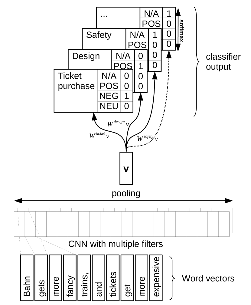
Figure 2: Schematic view of end-to-end CNN architecture.

Keeping the formalization as an end-to-end task, we replace the BiLSTM by a convolutional neural network (CNN) as described in Kim (2014). As in their setting CNN-non-static, we use $300$-dimensional word embeddings, a max-over-time pooling operation, filter sizes of $3,4,5$, and dropout with a rate of $0.5$ (as before). We use ReLu ($f(x)=\textit{max}(0,x)$) as our activation function, and $300$ filters of each size, a number also found in related work on sentiment analysis dos Santos and Gatti (2014). Following Kim (2014), we do not apply dropout after the embedding layer:

$$\mathbf{v}=\textit{DO}(\textit{CNN}(\textit{embed}(X)))$$ (7)

With Equation 7 replacing Equation 1, the aspectwise classification for the end-to-end CNN then follows the same definitions as described in the previous section.

3.5 Pipeline CNN

In order to compare the effects of joint end-to-end and pipeline approaches across neural architectures, we also include an experiment where the CNN model from the previous section replaces the BiLSTM in the pipeline setting described in section 3.2.

4 Experiments

We conduct our experiments on the GermEval 2017 data Wojatzki et al. (2017), i.e. customer feedback about Deutsche Bahn AG on social media, microblogs, news, and Q&A sites. The data were collected over the time of one year and manually annotated, resulting in a main dataset of about 26K documents, divided into a training, development, and test set using a random 80%/10%/10% split. About 1,800 documents from the last 3 months of the data collection period constitute a diachronic test set that can be used to test the robustness of a system over time. We keep the proposed data split and filter out training instances where the same aspect category was assigned two different polarity classes (which affects approximately $4\%{}$ of the data). The development and test data remain the same.

		development set	synchronic test set	diachronic test set
Pipeline LSTM	+ word2vec	.350	.297	.342
End-to-end LSTM	+ word2vec	.378	.315	.383
Pipeline CNN	+ word2vec	.350	.298	.343
End-to-end CNN	+ word2vec	.400	.319	.388
Pipeline LSTM	+ glove	.350	.297	.342
End-to-end LSTM	+ glove	.378	.315	.384
Pipeline CNN	+ glove	.350	.298	.342
End-to-end CNN	+ glove	.415	.315	.390
Pipeline LSTM	+ fasttext	.350	.297	.342
End-to-end LSTM	+ fasttext	.378	.315	.384
Pipeline CNN	+ fasttext	.342	.295	.342
End-to-end CNN	+ fasttext	.511	.423	.465
majority class baseline		–	.315	.384
GermEval baseline		–	.322	.389
GermEval best submission		–	.354	.401

Table 1: Results on the GermEval data, aspect + sentiment task. Micro-averaged F1-scores for both aspect category and aspect polarity classification as computed by the GermEval evaluation script. In the bottom part of the table, we report results from Wojatzki et al. (2017).

		development set	synchronic test set	diachronic test set
End-to-end LSTM	+ word2vec	.517	.442	.455
End-to-end CNN	+ word2vec	.521	.436	.470
End-to-end LSTM	+ glove	.517	.442	.456
End-to-end CNN	+ glove	.537	.457	.480
End-to-end LSTM	+ fasttext	.517	.442	.456
End-to-end CNN	+ fasttext	.623	.523	.557
majority class baseline		–	.442	.456
GermEval baseline		–	.481	.495
GermEval best submission		–	.482	.460

Table 2: Micro-averaged F1-scores for the prediction of aspect categories only (i.e. without taking polarity into account at all) as computed by the GermEval evaluation script. The results in the bottom part of the table are taken from Wojatzki et al. (2017).

We choose our hyperparameters based on the development data using the following procedure: we train initial models with a hyperparameter setting based on values we found in the literature, stochastic gradient descent with a learning rate of $0.01$ (as in dos Santos and Gatti (2014)) and a mini-batch size of $10$ (as in Ruder et al. (2016)). For the best-performing CNN and LSTM architectures (end-to-end + fasttext), we then refine the learning rate and batch size on the development data using random search in the range $\left\{\,0.001,0.003,0.01,0.03,0.1\,\right\}$ for learning rate and $\left\{\,5,10,20\,\right\}$ for batch size. For the CNN setting, this results in a learning rate of $0.03$ and a batch size of $5$ (which we then use for all CNN architectures in the final experiments). For the LSTM setting, this results in a learning rate of $0.01$ and a batch size of $10$ (which we then use for all LSTM architectures).

Training our models takes between 1-3 minutes per epoch on a GeForce GTX 1080 GPU, the end-to-end CNN being the fastest model to train.

5 Discussion

Aspect polarity

Table 1 shows the results of our experiments, as well as the results of our strong baselines. Note that the majority class baseline already provides good results. This is due to highly unbalanced data; the aspect category “Allgemein” (“general”), e.g., constitutes 61.5% of the cases. This imbalance makes the task even more challenging.

Over all architectures, we observe a comparable or better performance when using fasttext embeddings instead of word2vec or glove. This backs our hypothesis that subword features are important for processing the morphologically rich German language. Leaving everything else unchanged, we can furthermore see an increase in performance for all settings, when switching from the pipeline to an end-to-end approach. The best performance (marked in bold) is achieved by a combination of CNN and FastText embeddings, which outperforms the highly adapted winning system of the shared task.

Aspect category only

Even though our architectures are designed for the task of joint prediction of aspect category and polarity, we can also evaluate them on the detection of aspect categories only. Table 2 shows the results for this task. First of all, we can see that the SVM-based GermEval baseline model has very decent performance as it is practically on par with the best submission for the synchronic and even outperforms the best submission on the diachronic test set. It is therefore well-suited to serve as input to the pipeline LSTM model we compare with in our main task.

Comparing our architectures, we see again that fasttext embeddings always lead to equal or better performance. And even though we do not directly optimize our models for this task only, our best model (CNN+fasttext) outperforms all baselines, as well as the GermEval winning system.

Impact of domain-specific corpus

We compare the domain-specific FastText embeddings to FastText embeddings trained on Wikipedia, which is approximately 100 times the size of our domain-specific corpus. We report the results in Table 3. The embeddings trained on Wikipedia show slightly lower performance on the dev set but slightly higher or equal performance on the test sets. We conclude that the main positive impact of FastText stems from its capability to model subword information and that a large domain-independent corpus or a small domain-specific corpus lead to similar performance gains.

	dev	synchr. test	diachr. test
aspect + sent.	.502	.423	.465
aspect only	.610	.544	.571

Table 3: Results of the end-to-end CNN model with fasttext embeddings trained on the German Wikipedia.

6 Conclusion

We have presented a new approach to ABSA. By solving the two classification problems (aspect categories + aspect polarity) inherent to ABSA in a joint manner, we observe significant performance gains for both of these tasks on the GermEval 2017 data. Our experiments also showed that word representations leveraging subword information are crucial for a challenging task like ABSA in a morphologically rich language, such as German. Furthermore we observed consistently better performance of CNN architectures in otherwise comparable scenarios, which suggests that CNNs cope better with the irregularities of user-written texts on social media, a research question we leave to future work. By establishing a new state of the art in aspect detection and polarity classification, we provide a new practical baseline for future research in this area.

References

- Al-Rfou et al. (2013) Rami Al-Rfou, Bryan Perozzi, and Steven Skiena. 2013. Polyglot: Distributed word representations for multilingual nlp. In Proceedings of the Seventeenth Conference on Computational Natural Language Learning, pages 183–192, Sofia, Bulgaria. Association for Computational Linguistics.
- Brun et al. (2016) Caroline Brun, Julien Perez, and Claude Roux. 2016. XRCE at semeval-2016 task 5: Feedbacked ensemble modeling on syntactico-semantic knowledge for aspect based sentiment analysis. In Proceedings of the 10th International Workshop on Semantic Evaluation, SemEval@NAACL-HLT 2016, San Diego, CA, USA, June 16-17, 2016, pages 277–281.
- Grave et al. (2017) Edouard Grave, Tomas Mikolov, Armand Joulin, and Piotr Bojanowski. 2017. Bag of tricks for efficient text classification. In EACL (2), pages 427–431. Association for Computational Linguistics.
- Hinton et al. (2012) Geoffrey E. Hinton, Nitish Srivastava, Alex Krizhevsky, Ilya Sutskever, and Ruslan Salakhutdinov. 2012. Improving neural networks by preventing co-adaptation of feature detectors. CoRR, abs/1207.0580.
- Hochreiter and Schmidhuber (1997) Sepp Hochreiter and Jürgen Schmidhuber. 1997. Long short-term memory. Neural Computation, 9(8):1735–1780.
- Kim (2014) Yoon Kim. 2014. Convolutional neural networks for sentence classification. In Proceedings of the 2014 Conference on Empirical Methods in Natural Language Processing, EMNLP 2014, October 25-29, 2014, Doha, Qatar, A meeting of SIGDAT, a Special Interest Group of the ACL, pages 1746–1751.
- Kumar et al. (2016) Ayush Kumar, Sarah Kohail, Amit Kumar, Asif Ekbal, and Chris Biemann. 2016. IIT-TUDA at semeval-2016 task 5: Beyond sentiment lexicon: Combining domain dependency and distributional semantics features for aspect based sentiment analysis. In Proceedings of the 10th International Workshop on Semantic Evaluation, SemEval@NAACL-HLT 2016, San Diego, CA, USA, June 16-17, 2016, pages 1129–1135.
- Lee et al. (2017) Ji-Ung Lee, Steffen Eger, Johannes Daxenberger, and Iryna Gurevych. 2017. Ukp tu-da at germeval 2017: Deep learning for aspect based sentiment detection. In Proceedings of the GermEval 2017 – Shared Task on Aspect-based Sentiment in Social Media Customer Feedback, pages 22–29. German Society for Computational Linguistics.
- Mikolov et al. (2013) Tomas Mikolov, Kai Chen, Greg Corrado, and Jeffrey Dean. 2013. Efficient estimation of word representations in vector space. CoRR, abs/1301.3781.
- Pang and Lee (2008) Bo Pang and Lillian Lee. 2008. Opinion mining and sentiment analysis. Foundations and Trends in Information Retrieval, 2(1-2):1–135.
- Pennington et al. (2014) Jeffrey Pennington, Richard Socher, and Christopher D. Manning. 2014. Glove: Global vectors for word representation. In Empirical Methods in Natural Language Processing (EMNLP), pages 1532–1543.
- Pontiki et al. (2016) Maria Pontiki, Dimitris Galanis, Haris Papageorgiou, Ion Androutsopoulos, Suresh Manandhar, Mohammad AL-Smadi, Mahmoud Al-Ayyoub, Yanyan Zhao, Bing Qin, Orphee De Clercq, Veronique Hoste, Marianna Apidianaki, Xavier Tannier, Natalia Loukachevitch, Evgeniy Kotelnikov, Núria Bel, Salud María Jiménez-Zafra, and Gülşen Eryiğit. 2016. Semeval-2016 task 5: Aspect based sentiment analysis. In Proceedings of the 10th International Workshop on Semantic Evaluation (SemEval-2016), pages 19–30, San Diego, California. Association for Computational Linguistics.
- Ruder et al. (2016) Sebastian Ruder, Parsa Ghaffari, and John G. Breslin. 2016. A hierarchical model of reviews for aspect-based sentiment analysis. In Proceedings of the 2016 Conference on Empirical Methods in Natural Language Processing, pages 999–1005. Association for Computational Linguistics.
- dos Santos and Gatti (2014) Cícero Nogueira dos Santos and Maira Gatti. 2014. Deep convolutional neural networks for sentiment analysis of short texts. In COLING, pages 69–78. ACL.
- Wojatzki et al. (2017) Michael Wojatzki, Eugen Ruppert, Sarah Holschneider, Torsten Zesch, and Chris Biemann. 2017. GermEval 2017: Shared Task on Aspect-based Sentiment in Social Media Customer Feedback. In Proceedings of the GermEval 2017 – Shared Task on Aspect-based Sentiment in Social Media Customer Feedback, pages 1–12, Berlin, Germany.