High precision renormalization of the flavour non-singlet Noether currents in lattice QCD with Wilson quarks

Abstract

We determine the non-perturbatively renormalized axial current for O($a$) improved lattice QCD with Wilson quarks. Our strategy is based on the chirally rotated Schrödinger functional and can be generalized to other finite (ratios of) renormalization constants which are traditionally obtained by imposing continuum chiral Ward identities as normalization conditions. Compared to the latter we achieve an error reduction by up to one order of magnitude. Our results have already enabled the setting of the scale for the ${N_{\rm f}}=2+1$ CLS ensembles [1] and are thus an essential ingredient for the recent $\alpha_{s}$ determination by the ALPHA collaboration [2]. In this paper we shortly review the strategy and present our results for both ${N_{\rm f}}=2$ and ${N_{\rm f}}=3$ lattice QCD, where we match the $\beta$-values of the CLS gauge configurations. In addition to the axial current renormalization, we also present precise results for the renormalized local vector current.

1 Introduction

Lattice regularizations with Wilson type fermions [3] are widely used in current lattice QCD simulations [4, 5, 6, 7, 8, 9, 10]. The ultra-locality of the action enables numerical efficiency and thus access to a wide range of lattice spacings and spatial volumes. Furthermore, Wilson fermions maintain the full flavour symmetry of the continuum action, as well as the discrete symmetries such as parity, charge conjugation and time reversal. Unitarity is either realized exactly, or, in the case of Symanzik-improved actions, approximately up to cutoff effects which vanish in the continuum limit.

The price to pay for these advantages consists in the explicit breaking of all chiral symmetries by the Wilson term in the action. Well-known consequences include the additive renormalization of quark masses, the mixing under renormalization of composite operators in different chiral multiplets and discretization effects linear in $a$, the lattice spacing. Furthermore, the Noether currents of chiral symmetry are no longer protected against renormalization.

The matrix elements of the axial Noether currents between pion or kaon states and the vacuum, parametrized by the decay constants $f_{\pi,K}$, e.g.

$$\langle 0|A_{\mu}^{ud}(0)|\pi^{-},{\bf p}\rangle=ip_{\mu}f_{\pi},\qquad A_{\mu}^{ud}(x)=\overline{\psi}_{u}(x)\gamma_{\mu}\gamma_{5}\psi_{d}(x),$$ (1.1)

can be related to the measured life times of pions and kaons. The decay constants are finite in the chiral limit, can be precisely measured in numerical simulations and are ideally suited to set the scale in physical units. In order to achieve this with Wilson quarks one needs to determine the correctly renormalized axial currents,

$$\left(A_{\rm R}\right)_{\mu}^{f_{1}f_{2}}(x)=Z_{\rm A}A_{\mu}^{f_{1}f_{2}},\qquad$$ (1.2)

(with flavour indices $f_{1,2}=u,d,s$), which are to be inserted into the matrix elements. Of course it is desirable that the error of the matrix elements is not dominated by the uncertainty of the current normalization constant.

Over the last 30 years many efforts have been made to control the consequences of explicit chiral symmetry breaking with Wilson quarks. The main strategy consists in imposing continuum chiral symmetry relations as normalization conditions at finite lattice spacing [11, 12]. This is usually done using chiral Ward identities, which follow from an infinitesimal chiral change of variables in the QCD path integral. An example is the PCAC relation which determines the additive quark mass renormalization constant, as the “critical value” of the bare mass parameter, where the axial current is conserved. The fact that chiral symmetry is fully recovered only in the continuum limit implies that the choice of normalization condition matters at the cutoff level; at a fixed value of the lattice spacing the numerical results may occasionally differ substantially between any two such choices. Rather than interpreting this scatter as a systematic error, the modern approach consists in choosing a particular normalization condition and in fixing all dimensionful parameters (such as momenta or distances or background fields) in terms of a physical scale. This defines a so-called “line of constant physics” (LCP), along which the continuum limit is taken. As the lattice spacing $a$ (or, equivalently, the bare coupling, $g_{0}^{2}=6/\beta$), is varied, this defines a function $Z_{\rm A}=Z_{\rm A}(\beta)$. Obviously, another choice for the LCP will result in a different function $Z^{\prime}_{\rm A}(\beta)$. However, their difference will be, within errors, a smooth function of $\beta$ which vanishes asymptotically $\propto a$ or $\propto a^{2}$ if O($a$) improvement is implemented. Hence, following a LCP ensures that cutoff effects are smooth functions of $\beta$ and the choice of LCP becomes irrelevant in the continuum limit. Adopting this viewpoint, the relevant systematic error is therefore determined by the precision to which a chosen LCP can be followed.

In this paper we apply a recently developed method to lattice QCD with ${N_{\rm f}}=2$ and ${N_{\rm f}}=3$ flavours, matching the lattice actions chosen by the CLS initiative [8, 10]. Our method is based on the chirally rotated Schödinger functional ($\chi{\rm SF}$) [13, 14]. The theoretical foundation of this framework has been explained in [14] and it has passed a number of perturbative and non-perturbative tests [15, 16, 17, 18, 19, 20]. In contrast to the Ward identity method the axial current renormalization conditions follow from a finite chiral rotation in the massless QCD path integral with Schrödinger functional (SF) boundary conditions. The renormalization constants are then obtained from ratios of simple 2-point functions. For the axial current, this represents a significant advantage over the Ward identity method [12, 21, 22] which involves 3- and 4-point functions. Hence, we observe a dramatic improvement in the attainable statistical precision for $Z_{\rm A}$ and some care is required to ensure that systematic errors are under control at a similar level of precision. We also discuss the normalization procedure for the local vector current. While flavour symmetry remains unbroken on the lattice with (mass-degenerate) Wilson quarks, the corresponding Noether current lives on neighbouring lattice points connected by a gauge link, so that the use of the local vector current is often more practical.

This paper is organized as follows: after a short reminder of the $\chi{\rm SF}$ correlation functions in the continuum and the normalization conditions derived from them in sect. 2, we define in sect. 3 a couple of different LCPs which we have followed. We then present the $Z_{\rm A}$ and $Z_{\rm V}$ determinations for lattice QCD with ${N_{\rm f}}=2$ and ${N_{\rm f}}=3$ quark flavours in sects. 4 and 5, respectively, together with various tests we have carried out. Sect. 6 contains a summary of the main results of this work and some concluding remarks. Finally, the paper ends with three technical appendices: appendix A collects the parameters and results of the simulations, appendix B provides a detailed discussion on the systematic error estimates for our determinations, and appendix C gathers our set of chosen fit functions which smoothly interpolate our $Z_{\rm A,V}$ results in $\beta$.

The main results for ${N_{\rm f}}=2$ are collected in table 4, while those for ${N_{\rm f}}=3$ are given in tables 6 and 7. These results can be directly applied to data obtained from the CLS 2- and 3-flavour configurations, respectively [8, 10]. The ${N_{\rm f}}=3$ results have, in fact, already been used, and enabled the precision CLS scale setting in ref. [1] and the accurate quark-mass renormalization of ref. [23].

2 Renormalization conditions from universality relations

2.1 The Schrödinger functional and chiral field rotations

We start by considering massless two-flavour continuum QCD. The Euclidean space-time is taken to be a hyper-cylinder of volume $L^{4}$ with Schrödinger functional boundary conditions [24, 25]. In particular, in the Euclidean time direction, the quark and anti-quark fields satisfy,

$$P_{+}\psi(x)|_{x_{0}=0}=0=\overline{\psi}(x)P_{-}|_{x_{0}=0},$$ (2.3)

and similarly at time $x_{0}=L$ with the change $P_{\pm}\rightarrow P_{\mp}$. The SU(2)$\times$SU(2) chiral and flavour symmetry leads to conserved isovector Noether currents, given by

$$A_{\mu}^{a}(x)=\overline{\psi}(x)\gamma_{\mu}\gamma_{5}\dfrac{\tau^{a}}{2}\psi(x),\qquad V_{\mu}^{a}(x)=\overline{\psi}(x)\gamma_{\mu}\dfrac{\tau^{a}}{2}\psi(x),$$ (2.4)

with Pauli matrices $\tau^{a}$ and isospin index $a=1,2,3$. SF correlation functions of these currents with isovector boundary sources ${\mathcal{O}}_{5}^{a}$ and ${\mathcal{O}}^{a}_{k}$ have been defined in [26, 27] and are given by

$$\langle A^{a}_{0}(x)\mathcal{O}^{b}_{5}\rangle=-\delta^{ab}f_{\rm A}(x_{0}),\qquad\sum_{k=1}^{3}\langle V^{a}_{k}(x)\mathcal{O}^{b}_{k}\rangle=-3\,\delta^{ab}k_{\rm V}(x_{0}).$$ (2.5)

Passing from the isospin notation to fields with definite flavour assignments,

$$A^{f_{1}f_{2}}_{\mu}(x)=\overline{\psi}{}_{f_{1}}(x)\gamma_{\mu}\gamma_{5}\psi_{f_{2}}(x),\qquad V^{f_{1}f_{2}}_{\mu}(x)=\overline{\psi}{}_{f_{1}}(x)\gamma_{\mu}\psi_{f_{2}}(x),$$ (2.6)

and similarly for the boundary sources, the correlation functions for isospin indices $a=1,2$, can be written in terms of the flavour off-diagonal fields,

$$f_{\rm A}(x_{0})=-{1\over 2}\langle A^{ud}_{0}(x)\mathcal{O}^{du}_{5}\rangle,\qquad k_{\rm V}(x_{0})=-{1\over 6}\sum_{k=1}^{3}\langle V_{k}^{ud}(x)\mathcal{O}^{du}_{k}\rangle\,.$$ (2.7)

For the flavour diagonal fields in the isospin $a=3$ components, e.g.

$$A_{\mu}^{3}=\hbox{$1\over 2$}\left(A_{\mu}^{uu}-A_{\mu}^{dd}\right),$$ (2.8)

one may use flavour symmetry to write

$$f_{\rm A}(x_{0})=-\hbox{$1\over 2$}\langle A^{uu^{\prime}}_{0}(x)\mathcal{O}^{u^{\prime}u}_{5}\rangle,\quad$$ (2.9)

and analogously for $k_{\rm V}$. Note that the additional up-type flavour $u^{\prime}$ is merely a notational device to indicate the fermionic contractions taken into account when applying Wick’s theorem. Indeed, the sum of all the disconnected contributions for the flavour diagonal $a=3$ components of SF correlation functions cancels exactly due to flavour symmetry.

We now apply a flavour diagonal chiral rotation to the fields,

$$\psi\to\exp\left(i\dfrac{\alpha}{2}\gamma_{5}\tau^{3}\right)\psi,\qquad\overline{\psi}\to\overline{\psi}\exp\left(i\dfrac{\alpha}{2}\gamma_{5}\tau^{3}\right).$$ (2.10)

Choosing the rotation angle $\alpha=\pi/2$ then leads to the chirally rotated SF boundary conditions,

$$\tilde{Q}_{+}\psi(x)|_{x_{0}=0}=0=\overline{\psi}(x)\tilde{Q}_{+}|_{x_{0}=0},$$ (2.11)

with projectors $\tilde{Q}_{\pm}=\hbox{$1\over 2$}(1\pm i\gamma_{0}\gamma_{5}\tau^{3})$. Analogous boundary conditions with reverted projectors are obtained at $x_{0}=L$. Applying the same chiral field rotation to the axial currents,

$$A^{ud}_{\mu}(x)\to-iV^{ud}_{\mu}(x),\qquad A^{uu}_{\mu}(x)\to A^{uu}_{\mu}(x),$$ (2.12)

one obtains either a vector current or remains with an axial current, depending on the flavour assignments. If the chiral rotation of the field variables is performed as a change of variables in the functional integral, one arrives at the formal continuum identities

$$f_{\rm A}=g^{uu^{\prime}}_{\rm A}=-ig^{ud}_{\rm V},\qquad k_{\rm V}=l^{uu^{\prime}}_{\rm V}=-il^{ud}_{\rm A},$$ (2.13)

where the $g$- and $l$-functions are defined with $\chi$SF boundary conditions, eqs. (2.11), for instance

$$g_{\rm A}^{f_{1}f_{2}}(x_{0})=-\hbox{$1\over 2$}\langle A^{f_{1}f_{2}}_{0}(x)\mathcal{Q}^{f_{2}f_{1}}_{5}\rangle_{({\tilde{Q}}_{+})}\,.$$ (2.14)

Here, the boundary operators $\mathcal{Q}^{f_{1}f_{2}}_{5}$ denote the chirally rotated versions of their SF counterparts, $\mathcal{O}^{f_{1}f_{2}}_{5}$. For the complete expressions and further details we refer to ref. [20].

Regarding the case of QCD with ${N_{\rm f}}=3$ quark flavours we note that the very same steps can be taken provided the massless third quark does not take part in the chiral rotation and thus remains with standard SF boundary conditions [14]. Correlation functions are then considered for the doublet fields only, i.e. the third quark never appears as a valence quark.

2.2 Renormalization conditions

In the lattice regularized theory with Wilson type quarks, relations such as (2.13) can only be expected to hold after renormalization and up to cutoff effects. One first has to ensure that massless QCD with $\chi{\rm SF}$ boundary conditions has been correctly regularized. This is achieved by tuning the bare mass parameter $m_{0}$ to its critical value, $m_{\rm cr}$, where the axial current is conserved, and by tuning a boundary counterterm coefficient $z_{f}$ such that physical parity is restored (cf. [20] for more details). In terms of the bare $\chi$SF correlation functions one may choose the two conditions,

$$m={\tilde{\partial}_{0}g_{\rm A}^{ud}(x_{0})\over 2g_{\rm P}^{ud}(x_{0})}\bigg{|}_{x_{0}=L/2}=0,\qquad g_{\rm A}^{ud}(L/2)=0$$ (2.15)

(with $\tilde{\partial}_{0}$ the symmetric lattice derivative). The division by the pseudo-scalar correlation function $g_{\rm P}^{ud}$ is not really necessary, however it is done for convenience, as it gives rise to the definition of a (bare) PCAC quark mass $m$. Solutions to these equations define $m_{\rm cr}$ and $z_{f}^{*}$ as functions of the bare coupling $g_{0}$, and the lattice size, $L/a$.

Once the lattice regularization is correctly implemented, we expect e.g.

$$Z_{\rm A}Z_{\zeta}^{2}g^{uu^{\prime}}_{\rm A}(x_{0})=-iZ_{\rm V}Z_{\zeta}^{2}g^{ud}_{\rm V}(x_{0})+{\rm O}(a^{2}),$$ (2.16)

where $Z_{\zeta}$ renormalizes a boundary quark or anti-quark field [28, 26, 14] and $Z_{\rm A,V}$ are the current normalization constants of interest. Requiring such identities to hold exactly at finite lattice spacing thus fixes the relative normalization of axial and vector current. Replacing the latter by the exactly conserved lattice vector current ${\widetilde{V}}_{\mu}(x)$ (cf. ref. [20]), for which $Z_{\rm\widetilde{V}}=1$, one may obtain $Z_{\rm A}$ from either one of the ratios

$$R^{g}_{\rm A}={-ig_{\rm\widetilde{V}}^{ud}(x_{0})\over\phantom{-i}g_{\rm A}^{uu^{\prime}}(x_{0})}\bigg{|}_{x_{0}=L/2}\qquad\text{or}\qquad R^{l}_{\rm A}={il_{\rm\widetilde{V}}^{uu^{\prime}}(x_{0})\over\phantom{i}l_{\rm A}^{ud}(x_{0})}\bigg{|}_{x_{0}=L/2}.$$ (2.17)

Assuming that the parameters $x_{0}$ (here set to $L/2$), the boundary angle $\theta$ [29], the background gauge field [24], and the precise definition for the zero mass and $\alpha=\pi/2$ point (2.15) are fixed, we define, on an $(L/a)^{4}$ lattice and for a given bare coupling $g_{0}^{2}=6/\beta$,

$$Z^{g,l}_{\rm A}(\beta,L/a)=R^{g,l}_{\rm A}.$$ (2.18)

Finally the choice of a line of constant physics (cf. section 3) defines a smooth function $(L/a)(\beta)$ such that the normalization constants become functions of $\beta$ alone, with the difference between any two definitions vanishing smoothly with a rate $\propto a^{2}$.

We also comment on the appearance of a second up-type flavour $u^{\prime}$ in (2.17). When applying the chiral rotation (2.10) to the diagonal components of $f_{\rm A}$, the disconnected diagrams are mapped to disconnected diagrams on the $\chi$SF side which can be shown to add up to a pure cutoff effect. Their omission is thus perfectly legitimate, even if the formulation of the renormalization conditions then has an element of partial quenching to it. The situation is comparable with the Ward identity method in two-flavour QCD [12, 21], where a fictitious $s$-quark can be introduced to eliminate the disconnected diagrams.

Even though there exists a conserved vector current, in practice the local current is often used and then requires renormalization, too. Its renormalization constant can be obtained from,

$$R^{g}_{\rm V}={g_{\rm\widetilde{V}}^{ud}(x_{0})\over g_{\rm V}^{ud}(x_{0})}\bigg{|}_{x_{0}=L/2}\qquad\text{or}\qquad R^{l}_{\rm V}={l_{\rm\widetilde{V}}^{uu^{\prime}}(x_{0})\over l_{\rm V}^{uu^{\prime}}(x_{0})}\bigg{|}_{x_{0}=L/2}.$$ (2.19)

The same remarks as for the axial current normalization apply here, and with definite choices for all parameters we set,

$$Z^{g,l}_{\rm V}(\beta,L/a)=R^{g,l}_{\rm V}.$$ (2.20)

As in the case of the axial current normalization conditions, only 2-point functions are required, which connect the boundary quark bilinear sources with the currents in the bulk. This is a major advantage over the Ward identity method [12, 21] where 3- and 4-point functions are required. Hence, one expects better statistical precision from the simpler 2-point functions, and this will be confirmed below. Furthermore, as discussed in [20], the cutoff effects in the ratios are O($a^{2}$), due to the mechanism of automatic O($a$) improvement [30], even if the PCAC mass and the axial current are not O($a$) improved by the counterterm $\propto c_{\rm A}$ [26], or if the vector currents are not improved by the corresponding counterterms $\propto c_{\rm V},c_{\rm\widetilde{V}}$ [27, 31].

Finally, we emphasize that similar renormalization conditions can be devised for other finite renormalization constants. An interesting example is the ratio $Z_{\rm P}/Z_{\rm S}$, where $Z_{\rm P}$ and $Z_{\rm S}$ are the pseudo-scalar and scalar renormalization constant, respectively. We refer the reader to ref. [20] for more details.

3 Lines of constant physics and choice of renormalization conditions

3.1 General considerations

A line of constant physics requires to specify a physical (length) scale $r$ which is kept fixed as the continuum limit is taken. A typical choice would be the pion decay constant, $r=1/f_{\pi}$, either at the physical quark masses or in the chiral limit. Once calculated for a range of lattice spacings, this scale defines a function $(r/a)(\beta)$ of the bare coupling $\beta=6/g_{0}^{2}$ which fixes the lattice spacing $a$ in units of the chosen physical scale. Choosing the spatial lattice extent $L/a$, at a given beta, such that

$$\dfrac{(L/a)(\beta)}{(r/a)(\beta)}=L/r=C_{r}$$ (3.21)

(with a numerical constant $C_{r}$) then fixes the spatial size of the finite volume system in units of $r$. In practice we will choose $C_{r}$ such that the physical size of $L$ will be somewhat larger than half a femto metre. Note that this equation can be read in two ways: first, if one fixes $C_{r}$ and then chooses a set of $\beta$-values for which $r/a$ is known, one obtains a corresponding set of values $(L/a)(\beta)$, which will not necessarily be integers. To evaluate the normalization constants at these non-integer lattice sizes then requires some interpolation of results from neighbouring integer $L/a$-values at the same $\beta$. Alternatively, one could choose a set of integer $L/a$-values such that a choice for $C_{r}$ will imply a set of $\beta$-values. In general this means that the data for $r/a$ may have to be interpolated in $\beta$. We will here choose the first option, with the set of $\beta$-values taken over from the large volume simulations by the CLS project [8, 10].

Having set the scale one needs to ensure the correlation functions are calculated in the desired situation of massless QCD and for the chosen chirally rotated boundary conditions at $\alpha=\pi/2$. This means one needs to tune the bare quark mass $am_{0}$ and $z_{f}$ as functions of $\beta$. We will discuss this in more detail below. Finally, the correlation functions depend on kinematic parameters, such as $x_{0}$ or background field parameters such as $\theta$. We have already set $x_{0}=L/2$ in eqs. (2.17,2.19) and we choose $\theta=0$ and work with vanishing SU(3) background field.

With these parameter choices we will have, for a given $r$ and $C_{r}$ in eq. (3.21), two definitions each for $Z_{\rm A}$ and $Z_{\rm V}$, namely

$$Z^{g,l}_{\rm A,V}(\beta)=R_{\rm A,V}^{g,l}(\beta,a/L)\big{|}_{L/r=C_{r};\,m=0;\,\alpha=\pi/2}\,,$$ (3.22)

either based on the $g$- or the $l$-ratios. We then expect e.g. that

$$Z_{\rm A}^{g}(\beta)=Z_{\rm A}^{l}(\beta)+{\rm O}(a^{2}),$$ (3.23)

where the $a^{2}$-effects are now expected to be smooth functions of the bare coupling.

3.2 Perturbative subtraction of cutoff effects

A possible refinement consists in using perturbation theory to reduce the cutoff effects perturbatively. This requires to compute the $R$-ratios (2.17,2.19) perturbatively, with the exact same parameter choices as in the numerical simulations. We have performed this calculation to 1-loop order,

$$R_{\rm A,V}^{g,l}(g_{0}^{2},a/L)=R_{\rm A,V}^{g,l(0)}(a/L)+g_{0}^{2}R_{\rm A,V}^{g,l(1)}(a/L)+{\rm O}(g_{0}^{4}),$$ (3.24)

and for the chosen parameters we always find $R_{\rm A,V}^{g,l(0)}(a/L)=1$, exactly. We may then define a 1-loop correction factor,

$$r^{g,l}_{\rm A,V}(\beta,L/a)=\dfrac{1+g_{0}^{2}R_{\rm A,V}^{g,l(1)}(0)}{1+g_{0}^{2}R_{\rm A,V}^{g,l(1)}(a/L)}\,,$$ (3.25)

and results for the coefficients $R_{\rm A,V}^{g,l(1)}$ are collected in table 1, for the relevant lattice resolutions $L/a$ and the two lattice gauge actions used by CLS. Note that the 1-loop results are ${N_{\rm f}}$-independent and are thus obtained along the lines of ref. [20], the only difference being the form of the free gluon propagator in the case of the Lüscher-Weisz gauge action [32]. As an aside we note that our results converge to the known 1-loop results $Z_{\rm A,V}^{(1)}$ for an infinitely extended lattice [33, 34, 35], i.e. for $a/L=0$. We also observe that the 1-loop cutoff effects for the $l$-definitions are generally much smaller than for the $g$-definitions.

Wilson gauge action
$L/a$	$R_{\rm A}^{g(1)}(a/L)$	$R_{\rm A}^{l(1)}(a/L)$	$R_{\rm V}^{g(1)}(a/L)$	$R_{\rm V}^{l(1)}(a/L)$
6	$-0.104309$	$-0.116808$	$-0.118728$	$-0.130549$
8	$-0.109076$	$-0.116640$	$-0.122586$	$-0.129838$
10	$-0.111857$	$-0.116595$	$-0.125088$	$-0.129662$
12	$-0.113308$	$-0.116564$	$-0.126426$	$-0.129588$
16	$-0.114714$	$-0.116526$	$-0.127747$	$-0.129519$
$\infty$	$Z_{\rm A}^{(1)}=-0.116458(2)$		$Z_{\rm V}^{(1)}=-0.129430(2)$
Lüscher-Weisz gauge action
$L/a$	$R_{\rm A}^{g(1)}(a/L)$	$R_{\rm A}^{l(1)}(a/L)$	$R_{\rm V}^{g(1)}(a/L)$	$R_{\rm V}^{l(1)}(a/L)$
6	$-0.078368$	$-0.091011$	$-0.089760$	$-0.101750$
8	$-0.083286$	$-0.090737$	$-0.093819$	$-0.101006$
10	$-0.085958$	$-0.090650$	$-0.096256$	$-0.100811$
12	$-0.087374$	$-0.090604$	$-0.097578$	$-0.100730$
16	$-0.088756$	$-0.090557$	$-0.098889$	$-0.100657$
$\infty$	$Z_{\rm A}^{(1)}=-0.090488(5)$		$Z_{\rm V}^{(1)}=-0.100567(2)$

Table 1: Finite $L/a$ estimators for the current normalization constants at 1-loop order, and our estimates for their asymptotic values; the latter agree with previous results in the literature [33, 34, 35]. All results are given for ${\rm SU(3)}$.

For given $L/a$ and $\beta$, the perturbatively improved current normalization constants are now defined by

$$Z_{\rm A,V,\,sub}^{g,l}(\beta,L/a)=r_{\rm A,V}^{g,l}(\beta,L/a)\times Z_{{\rm A,V}}^{g,l}(\beta,L/a),$$ (3.26)

and, by construction, the O($a^{2}$) cutoff effects are subtracted to O($g_{0}^{2}$), reducing them to O($a^{2}g_{0}^{4}$). The subtracted data for the $Z$-factors are then treated as before: a choice of a line of constant physics implies a set of $\beta$- and corresponding $L/a$-values to which the data must be interpolated. We will see evidence for the effectiveness of this perturbative subtraction of cutoff effects in Sect. 4 and 5.

3.3 Choices of LCP for ${N_{\rm f}}=2$ and ${N_{\rm f}}=3$

In order to fix the physical scale $r$, we choose either the kaon decay constant $r=1/f_{K}$ (${N_{\rm f}}=2$), or the gradient flow scale $r=\sqrt{8t_{0}}$ (${N_{\rm f}}=3$) [36]. In order to fix the respective constants $C_{r}$ we proceed as follows. Given the set of values $\beta_{i}$ for $i=1,2,\ldots$ (taken from CLS), we choose as a reference value $\beta_{\rm ref}$ either the largest or the smallest of the set. Choosing an integer lattice size $L/a$ at the reference point $\beta_{\rm ref}$ now fixes $C_{r}$ through

$$C_{r}=\dfrac{(L/a)(\beta_{\rm ref})}{(r/a)(\beta_{\rm ref})}\,.$$ (3.27)

Having set the scale in this way, the $L/a$-values at the remaining $\beta_{i}$ follow from eq. (3.21). For all our choices the physical size of our space-time extent will be $L\approx 0.6-0.7\,{\rm fm}$. As mentioned before, except at the chosen reference value for $\beta$ this requires interpolations of simulation results at integer $L/a$ and our current simulation code, which is based on the openQCD package [37, 38], requires that $L/a$ is also even.

3.4 Topology freezing

Numerical simulations of the SF by means of standard Monte Carlo algorithms are known to suffer from the topology freezing problem (see e.g. ref. [39] for a discussion). A possible solution is to follow the proposal of ref. [39] and simulate the theory with open-SF boundary conditions. However, if for the given choice of parameters the problem is “mild”, one can circumvent the issue in a straightforward manner by simply imposing the renormalization conditions (2.20) and (2.15) within the trivial topological sector [40, 41]. In a continuum notation, the correlation functions entering these definitions are modified as follows,

$$g_{\rm A}^{ud}(x_{0})\,\to\,g_{\rm A,Q}^{ud}(x_{0})={-{1\over 2}\langle A^{ud}_{0}(x)\mathcal{Q}^{du}_{5}\delta_{Q,0}\rangle_{({\tilde{Q}}_{+})}\over\langle\delta_{Q,0}\rangle_{({\tilde{Q}}_{+})}},$$ (3.28)

and analogously in all other cases. Here, the Kronecker $\delta$ in the functional integral selects the gauge field configurations with topological charge $Q=0$. Since relations based on chiral flavour symmetries should hold separately in each topological charge sector, this restriction to the trivial sector is a legitimate modification of the current renormalization conditions. It provides a viable solution to the algorithmic problem of topology freezing in cases where this problem becomes marginally relevant; this means when the fraction of topologically non-trivial gauge field configurations in the relevant ensembles is not too large. For our choices of parameters, the percentage of gauge field configurations with $Q\neq 0$ is generally below 10%, and reaches approximately 30% only in a couple of cases (cf. tables 8 and 9).

On the lattice the topological charge is not unambiguously defined. We follow refs. [40, 41] and define the trivial topological sector as the set of gauge field configurations for which $|Q|<0.5$, where $Q$ is discretized in terms of the Wilson flow and the clover definition of the field strength tensor [36]. The flow time $t$ is then kept fixed in physical units by requiring $\sqrt{8t}=0.6\times L$.

3.5 On the tuning of $am_{0}$ and $z_{f}$

The current normalization conditions require the $\chi$SF correlation functions at zero quark mass and with a chiral twist angle of $\pi/2$. In practice this is achieved by the simultaneous tuning of $m_{0}$ and $z_{f}$ such that eqs. (2.15) are satisfied. In general a 2-parameter tuning can be quite involved. However, here the non-perturbative O($a$) improvement of the action implies that the O($a$) uncertainty of the zero mass point is very much reduced. Since a change in $z_{f}$ merely re-defines the matrix element used to define the PCAC mass, a variation of $z_{f}$ is expected to induce a small variation of $m$ within this O($a$) uncertainty. The latter could in principle be reduced to O($a^{2}$) by including the $c_{\rm A}$-counterterm to the axial current, but this will not be pursued here. Another important observation is that, once $m_{0}$ and $z_{f}$ are within O($a$) of their target values, the sensitivity of the PCAC mass to a variation of $z_{f}$ is reduced to order $a^{2}$ (cf. appendix B, discussion after eq. (B.44)). One is therefore led to conclude that the PCAC mass $m$ is to a good approximation independent of $z_{f}$, and the tuning of $m_{0}$ and $z_{f}$ thus becomes straightforward; given a reasonable guess for $z_{f}$, one can first tune $m_{0}$, and then turn to $z_{f}$.

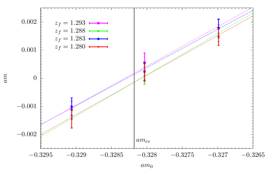
Figure 1: Results for the PCAC mass as a function of the bare quark mass, for different values of $z_{f}$. The dashed lines are linear fits to the data, while the solid vertical line indicates the location of our final estimate for $am_{\rm cr}(g_{0},a/L)$ (s. main text). The results are for $L/a=8$ and $\beta=5.3$.

As an illustration of this situation we discuss the ${N_{\rm f}}=2$ case for $L/a=8$, $\beta=5.3$. For the tuning we considered 3 values of $\kappa=1/(2am_{0}+8)$ and 4 values of $z_{f}$. We then generated around 2000 gauge field configurations separated by 10 MDUs for each of the 12 ensembles, and measured the relevant correlation functions. Figure 1 collects the results for the PCAC mass as a function of the bare quark mass, for the 4 different values of $z_{f}$. Within statistical errors, the PCAC mass depends linearly on $m_{0}$ and is essentially independent of $z_{f}$. A linear fit of $m$ vs. $m_{0}$ yields an estimate of $m_{0}=m_{\rm cr}(g_{0},L/a)$ for which $m$ vanishes: these are collected in table 2. The results are perfectly compatible with each other, and we take as our estimate for $m_{\rm cr}$ the result of a weighted average of these four.

$z_{f}$	$am_{\rm cr}$	$\kappa_{\rm cr}$
$1.280$	$-0.32808(13)$	$0.1361685(47)$
$1.283$	$-0.32828(14)$	$0.1361761(51)$
$1.288$	$-0.32808(12)$	$0.1361687(45)$
$1.293$	$-0.32831(14)$	$0.1361772(51)$
average	$-0.328179(65)$	$0.1361722(24)$

Table 2: Results for $am_{\rm cr}(g_{0},L/a)$ for four different values of $z_{f}$, for $L/a=8$ and $\beta=5.3$. The weighted average of the results is also given in the last row of the table.

Once the critical bare mass is fixed, a smooth interpolation of $g_{\rm A}^{ud}(L/2)$ in $m_{0}$ gives the results shown in figure 2. Over the chosen range, $g_{\rm A}^{ud}(L/2)$ so interpolated is perfectly linear in $z_{f}$, and it is thus straightforward to determine the point $z_{f}^{*}$ where $g_{\rm A}^{ud}(L/2)$ vanishes i.e. $z^{*}_{f}=1.2877(5)$ in this example.

Figure 2: Results for $g_{\rm A}^{ud}(L/2)$ as a function of $z_{f}$. The dashed line is a linear fit to the data, while the solid vertical line indicates the location of our final estimate for $z_{f}^{*}$ (s. main text). The values of $g_{\rm A}^{ud}(L/2)$ come from an interpolation to $\kappa=0.1361722$, and are for $L/a=8$ and $\beta=5.3$.

The estimated values of $am_{\rm cr}$ and $z_{f}^{*}$ determined in this way turn out to be quite accurate in practice, cf. table 8. We remark that results for $m_{\rm cr}$ could also be taken from a different source, for instance from standard SF simulations. In this case only $z_{f}$ needs to be tuned. The differences to the above procedure would be O($a$) both in $m_{\rm cr}$ and in $z_{f}^{*}$ which, by the mechanism of automatic O($a$) improvement, induce O($a^{2}$) differences in observables such as the current normalization constants [14, 20]. One also expects that a precise tuning of $m_{0}$ is less crucial in the $\chi{\rm SF}$ than in the SF; the quark mass dependence of physical observables around the chiral limit is quadratic rather than linear [42].

3.6 Sources of uncertainties

Besides statistical errors directly affecting the estimators for the current normalization constants, the other source of uncertainty originates from the precision to which a line of constant physics can be followed. In principle also this latter effect is of a statistical nature, however, some elements of modelling or estimates may be involved when propagating these errors to the normalization constants, so that it is partly justified labelling these effects as systematic.

Our procedure consists of the following steps:

1. The LCP together with the set of values $\beta_{i}$ translates to target values $(L/a)(\beta_{i})$. At each $\beta_{i}$ we choose lattices with even $L/a$ straddling the target values. We here anticipate that with our choices of LCPs the required lattice sizes are in the range $L/a=8$ to $L/a=16$. Note that all target values $(L/a)(\beta_{i})$ come with statistical errors except for $\beta=\beta_{\rm ref}$, where, by definition, $L/a$ is given as an (even) integer.

2. For given $\beta$ and $L/a$ we determine the solutions $am_{0}=am_{\rm cr}$ and $z_{f}=z_{f}^{*}$ of eqs. (2.15). In order to find their statistical errors which follow from the statistical uncertainties on $m$ and $g_{\rm A}^{ud}(L/2)$, we use estimates for the relevant derivatives,

   $${\partial mL\over\partial m_{0}L},\quad{\partial mL\over\partial z_{f}},\quad{\partial g_{\rm A}^{ud}\over\partial m_{0}L},\quad{\partial g_{\rm A}^{ud}\over\partial z_{f}}.$$ (3.29)

3. We then determine the induced error on the $Z$-factors by estimating their derivatives with respect to the bare parameters,

   $${\partial Z_{\rm A,V}\over\partial z_{f}},\quad{\partial Z_{\rm A,V}\over\partial m_{0}L}.$$ (3.30)

   It turns out that the derivatives (3.29) and (3.30) scale quite well with lattice size and lattice spacing, so that it is unnecessary to evaluate them for all parameter choices. Some cross checks are sufficient. The errors coming from the uncertainties in $m_{0}$ and $z_{f}$ are then combined in quadrature and added, again in quadrature, to the statistical error.

4. Where necessary, the results for $Z_{\rm A,V}$ at the different $L/a$-values and fixed $\beta_{i}$ are interpolated to the target $(L/a)(\beta_{i})$; and the statistical error on $(L/a)(\beta_{i})$ is propagated at this point. In the case where only one value of $L/a$ has been simulated, an estimate for the derivative

   $${\partial Z_{\rm A,V}\over\partial(L/a)}$$ (3.31)

   is used to assign a systematic error due to the difference $\Delta(L/a)\equiv L/a-(L/a)(\beta_{i})$, also taking into account the statistical uncertainty on $(L/a)(\beta_{i})$. The resulting systematic error is again added in quadrature.

We emphasize that all systematic effects become essentially statistical errors provided enough data is produced to estimate the derivatives required to propagate the errors to the normalization constants. In the following two sections we will present the lattice set-up and results for ${N_{\rm f}}=2$ and ${N_{\rm f}}=3$ lattice QCD. We will also come back to some of the above points.

4 Numerical results for ${N_{\rm f}}=2$ flavours

4.1 Lattice set-up and parameter choices

The CLS large volume simulations of 2-flavour QCD [8] were performed using non-perturbatively O($a$) improved Wilson quarks and the Wilson gauge action. The matching to CLS data via the bare coupling requires that we use the same action in the $\chi$SF. As for the details of the action near the time boundaries we refer to ref. [20]. In particular the counterterm coefficients $c_{\rm t}(g_{0})$ and $d_{s}(g_{0})$ were set to their perturbative one-loop values using the results of that reference. In general, the incomplete cancellation of boundary O($a$) artefacts implies some remnant O($a$) effects in observables. However, for the estimators of the current normalization constants, eqs. (2.17,2.19), it can be shown that such O($a$) effects only cause O($a^{2}$) differences [20].

The CLS simulations were carried out for 3 values of the lattice spacing [8], corresponding to the $\beta$-values $5.2$, $5.3$ and $5.5$. For future applications we have added a finer lattice spacing corresponding to $\beta=5.7$. We choose the smallest CLS-value $\beta=5.2$ as reference value and set

$$L/a=8\quad{\rm at}\quad\beta=5.2,$$ (4.32)

to define the starting point for the line of constant physics. We then fix the space-time volume of the $\chi{\rm SF}$ simulations in terms of the kaon decay constant, $f_{K}$, evaluated at physical quark masses. Taking $af_{K}$ from table 3 at $\beta=5.2$ yields

$$f_{K}L=0.4744(74),$$ (4.33)

and corresponds to $L\approx 0.6\,{\rm fm}$. Imposing this condition at the other $\beta$-values then leads to the (non-integer) $L/a$-values given in table 3. The quoted errors are a combination of statistical uncertainties, propagated from eq. (4.33) and the error on $af_{K}$ at the given $\beta$’s.

$\beta$	$af_{K}$	$(L/a)(\beta)$	$L/a$
5.2	0.0593(7)(6)	8	8
5.3	0.0517(6)(6)	9.18(21)	8, 10, 12
5.5	0.0382(4)(3)	12.42(25)	12
5.7	0.0290(11)†	16.35(67)	16

• ^†This value is estimated using the perturbative running of the lattice spacing (s. main text).

Table 3: Values of $af_{K}$ used to determine $(L/a)(\beta)$ such as to satisfy the condition (4.33) for the given $\beta$. The $\chi{\rm SF}$ simulations were performed at the neighbouring even integer $L/a$-values given in the last column.

While the first 3 results for $af_{K}$ in table 3 have been directly measured [8] we have estimated $af_{K}$ at the fourth value, $\beta=5.7$, as follows: with $af_{K}$ at $\beta=5.5$ taken as starting point we used the three-loop $\beta$-function for the bare coupling [43], in order to determine the ratio of lattice spacings. The error is obtained by summing (in quadrature) the statistical error propagated from the result at $\beta=5.5$, and a systematic error due to the use of perturbation theory. The latter is estimated as the difference between the non-perturbative result for $af_{K}$ at $\beta=5.5$, and the same perturbative procedure, applied between $\beta=5.3$ and $\beta=5.5$. This systematic error is about 2.7 times larger than the statistical one, and thus dominates the error on $L/a$ at $\beta=5.7$.

Except for $\beta=5.3$, the target values $(L/a)(\beta_{i})$ resulting from condition (4.33), are very close to even integer values of $L/a$, so that interpolations between simulations at different $L/a$ can be avoided. At $\beta=5.3$ we simulated at the three $L/a$-values given in the last column of table 3 and interpolated to the target value (see appendix B.4 for more details). For each choice of $\beta$ and $L/a$, along the lines of the discussion in Sect. 3.5, we have carried out various tuning runs covering a range of $am_{0}$ and $z_{f}$, so as to determine the parameters satisfying the conditions (2.15). The values of the tuned parameters and the results for $m$ and $g_{\rm A}^{ud}(L/2)$ at these parameters are given in table 8.

4.2 Results and error budget

In table 4 we collect the results for $Z_{\rm A,V}$, both $g$ and $l$ definitions, at the four values of the lattice spacing. The statistics range from $1,800$ to $12,000$ measurements depending on the ensemble, cf. table 8. The quoted uncertainties combine the statistical and systematic errors. The statistical errors are at the level of $0.1-0.4\permil$, depending on the $Z$-factor and ensemble considered. Hence a significant contribution to the error comes from systematic uncertainties.

$\beta$	$Z_{\rm A}^{g}$	$Z_{\rm A}^{l}$	$Z_{\rm V}^{g}$	$Z_{\rm V}^{l}$
$5.2$	$0.78022(55)$	$0.76944(94)$	$0.74673(47)$	$0.73849(97)$
$5.3$	$0.78411(61)$	$0.77576(66)$	$0.75220(70)$	$0.74607(69)$
$5.5$	$0.7945(13)$	$0.7895(13)$	$0.7663(14)$	$0.7625(14)$
$5.7$	$0.80526(97)$	$0.80277(93)$	$0.7800(11)$	$0.77801(98)$
$\beta$	$Z_{\rm A,\,sub}^{g}$	$Z_{\rm A,\,sub}^{l}$	$Z_{\rm V,\,sub}^{g}$	$Z_{\rm V,\,sub}^{l}$
$5.2$	$0.77262(54)$	$0.76963(94)$	$0.73986(47)$	$0.73890(97)$
$5.3$	$0.77847(42)$	$0.77591(66)$	$0.74706(49)$	$0.74636(70)$
$5.5$	$0.79138(89)$	$0.7897(13)$	$0.7634(11)$	$0.7627(14)$
$5.7$	$0.80358(63)$	$0.80283(93)$	$0.77836(79)$	$0.7781(10)$

Table 4: Results for $Z_{\rm A,V}$, both $g$ and $l$ definitions, for ${N_{\rm f}}=2$ non-perturbatively O($a$) improved Wilson fermions and Wilson gauge action. The lower part of the table contains the same results after subtraction of the one-loop cutoff effects, cf. eq. (3.26).

As discussed in section 3.6, systematic errors result from uncertainties or deviations in following a chosen LCP, which correspond with statistical errors and deviations from zero in $m$ and $g_{\rm A}^{ud}(L/a)$, as well as uncertainties in the target lattice extent $L/a$ and systematic errors arising from inter- or extrapolations from the simulated lattices sizes, if applicable. Tables 3 and 8 contain the relevant information for the case ${N_{\rm f}}=2$. The propagation of these uncertainties to the $Z$-factors is then performed following the steps outlined in Sect. 3.6. We have carried out some additional simulations to estimate the derivatives in eqs. (3.29,3.30), and some perturbative calculation to check the expected scaling of the derivatives with the lattice size. We delegate a detailed discussion to appendix B. Here we just note that with our statistics and our rather conservative approach, the propagated uncertainties are typically larger than the statistical errors for the $R$-estimators eqs. (2.17,2.19) (cf. tables 11 and 11).

4.2.1 Effect of perturbative one-loop improvement

As discussed in section 3.2, we have also computed the relevant $\chi$SF correlation functions in perturbation theory to order $g_{0}^{2}=6/\beta$. Besides consistency checks and qualitative insight the main application consists in the perturbative subtraction of cutoff effects from the data. Note that this requires to emulate the non-perturbative procedure in all details, in particular the determination of $am_{\rm cr}$ and $z_{f}^{*}$ according to eqs. (2.15). The lower part of table 4 contains the results for $Z_{\rm A,V}$ after perturbative improvement. Comparing with the unimproved results in the upper part of table 4, one can see that the $g$-definitions are more affected, and are brought closer to the corresponding $l$-definitions by the perturbative improvement (cf. also figure 5). In any case, the perturbative corrections are at the level of 1 per cent at most.

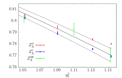
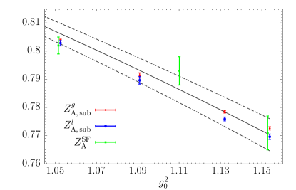
Figure 3: Comparison of different $Z_{\rm A}$ determinations for ${N_{\rm f}}=2$, obtained from WIs in the standard SF and from universality relations in the $\chi{\rm SF}$. The effect of the perturbative one-loop improvement of the $\chi{\rm SF}$ results is also shown (right panel). The $\chi{\rm SF}$ results are those of table 4. The individual SF points are taken from refs. [44, 8], and are slightly displaced on the $x$-axis for better clarity. The solid black line corresponds to the SF results from the fit formula of ref. [8], and the dashed lines delimit the $1\sigma$ region of the fit. Note that the SF fit formula is obtained by considering additional points with $g_{0}^{2}<1$, here not shown, and by enforcing the perturbative 1-loop behaviour for $g_{0}^{2}\to 0$ (see ref. [8] for the details).

In conclusion, our final results for $Z_{\rm A,V}$, either with or without perturbative improvement, turn out to be very precise and improve significantly on the standard SF determination based on chiral Ward identities (WIs) [21, 44, 8]. This is particularly true for the case of $Z_{\rm A}$, which can be appreciated in figure 3 where the determinations of table 4 are compared with those of refs. [44, 8]. In figure 4 we show instead a comparison for the case of $Z_{\rm V}$, as obtained from the $\chi{\rm SF}$, cf. table 4, and from the standard SF (cf. ref. [21]). We note that a relevant contribution to the error of our results comes from propagating the uncertainties associated with maintaining the condition (4.33) i.e. keeping $L$ constant (cf. table 11 and 11). We anticipate that due to the much more accurate knowledge of the LCP in terms of $t_{0}$ (cf. table 5), and by using interpolations in $L/a$ at all relevant $\beta$ values, this source of error will be essentially eliminated in the case of ${N_{\rm f}}=3$ (cf. section 5).

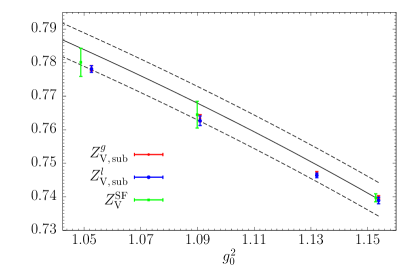
Figure 4: Comparison of different $Z_{\rm V}$ determinations for ${N_{\rm f}}=2$, obtained from WIs in the standard SF and from universality relations in the $\chi{\rm SF}$. The effect of the perturbative one-loop improvement of the $\chi{\rm SF}$ results is also shown (right panel). The $\chi{\rm SF}$ results are those of table 4. The individual SF points are taken from refs. [21], and are slightly displaced on the $x$-axis for better clarity. The solid black line corresponds to the SF results from the fit formula of ref. [21], and the dashed lines delimit the $1\sigma$ region of the fit. Note that the SF fit formula is obtained by considering additional points with $g_{0}^{2}<1$, here not shown, and by enforcing the perturbative 1-loop behaviour for $g_{0}^{2}\to 0$ (see ref. [21] for the details).

4.3 Universality and automatic O($a$) improvement

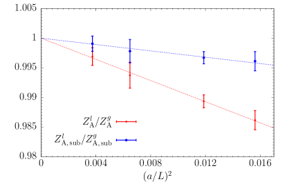
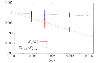
Figure 5: Continuum limit of the ratios between the $l$ and $g$ definitions of $Z_{\rm A}$ (left panel) and $Z_{\rm V}$ (right panel) for the case of ${N_{\rm f}}=2$ quark-flavours; the effect of subtracting the lattice artefacts from the $Z$-factors to O($g_{0}^{2}$) is also shown. The dashed lines correspond to linear fits to the data, constrained to extrapolate to 1 for $a/L=0$.

The $\chi{\rm SF}$ determinations (2.17) and (2.19) are expected to be automatically O($a$) improved once the bare parameters $m_{0}$ and $z_{f}$ are properly tuned (cf. section 2.2). This means that neither bulk nor boundary O($a$) counterterms are necessary to cancel O($a$) discretization errors in these quantities. This was confirmed to one-loop order in perturbation theory [20] and should hold generally. To this end we now look at the ratios between $Z$-factors coming from the $g$- and $l$-definitions. The expectation that these ratios converge to 1 with O($a^{2}$) corrections is indeed very well borne out by the data, cf. figure 5, where we also include fits to this expected behaviour. We emphasize that this is a non-trivial result: even though the bulk action is improved to match the CLS set-up, we did not O($a$) improve the currents entering the definitions (2.17,2.19) and (2.15). This result thus confirms automatic O($a$) improvement at the non-perturbative level, and, indirectly, the universality relations between the $\chi{\rm SF}$ and SF formulations. A direct way to test universality between the $\chi{\rm SF}$ and SF formulations would be simply to study the continuum scaling of ratios of $Z$-factors as obtained from one and the other formulation. Provided the SF determinations are properly improved, these should also approach 1 in the continuum limit with O($a^{2}$) corrections. The large errors on the SF determinations do not allow us for a precise test of this expectation. However, the results in figure 3 and 4 clearly show that our determinations are in fact compatible with the SF ones within errors.

5 Numerical results for ${N_{\rm f}}=3$ flavours

5.1 Lattice set-up and parameter choices

The CLS simulations with ${N_{\rm f}}=2+1$ flavours of non-perturbatively O($a$) improved Wilson fermions [45] and Lüscher-Weisz (LW) gauge action, have been carried out for 5 values of the lattice spacing, with $\beta$-values between $3.4$ and $3.85$ [10, 1, 2]. For completeness we note that CLS has also tried to simulate at a coarser lattice spacing corresponding to $\beta=3.3$. However, these ensembles have been discarded for the scale determination in [1] due to very large cutoff effects observed e.g. in $t_{0}$ [10]. For this reason we will not consider this $\beta$-value in our study, however, we mention that it was adopted as starting point for the Ward identity determination of $Z_{\rm A}$ in ref. [22]. Given the relatively large set of lattice spacings we here consider two different LCPs, with slightly different physical extent, $L_{1}$ and $L_{2}$, which we define through the gradient flow time $t_{0}$ [36]. The associated length scale $r=\sqrt{8t_{0}}$ can be interpreted as a smoothing radius, and has been very precisely determined for the CLS $\beta$-values $\geq 3.4$ in [1, 2]. Using this scale we impose the conditions

$$L_{1}/\sqrt{8t_{0}}=1.6719(16)\quad{\rm and}\quad L_{2}/\sqrt{8t_{0}}=1.5099(30),$$ (5.34)

where the right hand sides were chosen in order to have exactly,

$$L_{1}/a=8\quad{\rm at}\quad\beta=3.4\quad{\rm and}\quad L_{2}/a=16\quad{\rm at}\quad\beta=3.85,$$ (5.35)

respectively. Using the result for $t_{0}$ in physical units [1], eqs. (5.34) translate to $L_{1}\approx 0.7\,{\rm fm}$ and $L_{2}\approx 0.6\,{\rm fm}$.

$\beta$	$t_{0}/a^{2}$	$(L_{1}/a)(\beta)$	$(L_{2}/a)(\beta)$	$L/a$
$3.40$	$2.8619(55)$	$8$	$7.225(16)$	$6$, $8$, $10$, $12$
$3.46$	$3.662(13)$	$9.049(18)$	$8.172(22)$	$6$, $8$, $10$, $12$
$3.55$	$5.166(17)$	$10.748(21)$	$9.706(25)$	$8$, $10$, $12$, $16$
$3.70$	$8.596(31)$	$13.864(29)$	$12.521(34)$	$8$, $10$, $12$, $16$
$3.85$	$14.036(57)$	$-$	$16$	$16$

Table 5: CLS $\beta$-values and corresponding results for $t_{0}/a^{2}$ in the SU(3) flavour symmetric limit [1, 2]. The latter are used to determine the lattice sizes $(L_{1,2}/a)(\beta_{i})$ which satisfy the conditions (5.34). The $\chi{\rm SF}$ simulations are performed at the neighbouring $L/a$’s given in the last column of the table.

In table 5 we collect the relevant $\beta$ values of the CLS simulations and the corresponding results for $t_{0}/a^{2}$ [2]. The latter are evaluated for equal up-, down-, and strange-quark masses, which are close to the physical average quark mass (see refs. [1, 2]). Table 5 also gives the lattice sizes $(L_{1,2}/a)(\beta)$ which satisfy the conditions (5.34). Compared to the ${N_{\rm f}}=2$ case (cf. table 3), it is obvious that these ${N_{\rm f}}=3$ LCPs are much more accurately determined. In order to exploit this higher precision, we performed simulations for several $L/a$-values at each $\beta$ (cf. table 5). This allowed us to accurately interpolate the $Z$-factors to the target values (see appendix B.5 for more details). Table 9 contains a summary of all simulations performed with the corresponding parameters. Due to both technical and historical reasons, we do not use the finest lattice spacing for the LCP defined in terms of $L_{1}$. Following this LCP up to $\beta=3.85$ would have required simulating lattices with $L/a=18,20$, which are particularly inconvenient to parellelize with our current simulation program. Note also that CLS simulations at $\beta=3.85$ are ongoing and currently limited to a single ensemble, so that the LCP with $L_{1}$ may remain useful for a while. More importantly, however, the comparison between both LCPs allows us to perform additional tests on our results (cf. section 5.3).

The lattice action we employ for the finite volume simulations matches the CLS action in the bulk, i.e. the Lüscher-Weisz tree-level improved gauge action and 3 flavours of non-perturbatively improved Wilson quarks [45]. Close to the time boundaries of the lattice there is some freedom regarding the implementation of Schrödinger functional boundary conditions. For the gauge fields we choose option B of ref. [32]; we refer the reader to this reference for the details. Regarding the fermions, two quark flavours satisfy $\chi{\rm SF}$ boundary conditions (option $\tau=1$ of [14]), while the third one obeys the standard SF boundary conditions [25]. In general, such a mixed set-up increases the number of O($a$) improvement coefficients which need to be tuned in order to eliminate O($a$) discretization errors from the time boundaries. As in the ${N_{\rm f}}=2$ case, however, one can show that the corresponding counterterms affect the renormalization constants $Z_{\rm A,V}$ only at O($a^{2}$). For definiteness we have used the one-loop estimate $c_{\rm t}=1+g_{0}^{2}c_{\rm t}^{(1)}$, where the one-loop coefficient decomposes as follows,

$$c_{\rm t}^{(1)}=c_{\rm t}^{(1,0)}+2\times c_{\rm t}^{(1,1)}(\text{$\chi$SF})+1\times c_{\rm t}^{(1,1)}(\text{SF}).$$ (5.36)

The pure gauge contribution is taken from ref. [46], the fermionic $\chi{\rm SF}$ contribution from ref. [20] and the SF contribution from ref. [29]. Furthermore, we use the tree-level values $d_{s}=1/2$ [20] and $\tilde{c}_{\rm t}=1$ [26].

5.2 Results and error budget

In table 6 and 7 we collect the results for $Z_{\rm A,V}$, corresponding to the $L_{1}$- and $L_{2}$-LCP, respectively. The statistics we accumulated for the different ensembles ranges between 3,200 and 31,000 measurements, with exact numbers given in table 9. The corresponding statistical precision on the $Z$-factors is between $0.1-0.55\permil$, depending on the exact quantity and ensemble. The errors quoted in the tables then combine the statistical errors with the systematic errors originating from the uncertainties on the LPCs.

$\beta$	$Z_{\rm A}^{g}$	$Z_{\rm A}^{l}$	$Z_{\rm V}^{g}$	$Z_{\rm V}^{l}$
$3.40$	$0.76847(35)$	$0.75446(68)$	$0.72923(27)$	$0.71940(70)$
$3.46$	$0.77128(44)$	$0.76018(80)$	$0.73392(36)$	$0.72637(77)$
$3.55$	$0.77703(30)$	$0.76879(42)$	$0.74261(23)$	$0.73758(44)$
$3.70$	$0.78831(30)$	$0.78327(43)$	$0.75833(31)$	$0.75521(44)$
$\beta$	$Z_{\rm A,\,sub}^{g}$	$Z_{\rm A,\,sub}^{l}$	$Z_{\rm V,\,sub}^{g}$	$Z_{\rm V,\,sub}^{l}$
$3.40$	$0.75702(35)$	$0.75485(68)$	$0.71882(27)$	$0.72008(70)$
$3.46$	$0.76245(44)$	$0.76048(80)$	$0.72578(36)$	$0.72683(77)$
$3.55$	$0.77103(29)$	$0.76900(42)$	$0.73701(23)$	$0.73789(44)$
$3.70$	$0.78485(30)$	$0.78340(43)$	$0.75506(31)$	$0.75538(44)$

Table 6: ${N_{\rm f}}=3$ results for $Z_{\rm A,V}$ using the $L_{1}$-LCP, both for $g$ and $l$ definitions. The lower part of the table contains the results after subtraction of the one-loop cutoff effects, cf. eq. (3.26).

$\beta$	$Z_{\rm A}^{g}$	$Z_{\rm A}^{l}$	$Z_{\rm V}^{g}$	$Z_{\rm V}^{l}$
$3.40$	$0.77129(39)$	$0.75592(72)$	$0.73368(30)$	$0.72164(74)$
$3.46$	$0.77371(51)$	$0.76132(93)$	$0.73721(42)$	$0.72782(89)$
$3.55$	$0.77856(31)$	$0.76953(43)$	$0.74468(25)$	$0.73846(46)$
$3.70$	$0.78925(31)$	$0.78362(47)$	$0.75936(33)$	$0.75552(48)$
$3.85$	$0.79985(31)$	$0.79657(47)$	$0.77304(33)$	$0.77061(49)$
$\beta$	$Z_{\rm A,\,sub}^{g}$	$Z_{\rm A,\,sub}^{l}$	$Z_{\rm V,\,sub}^{g}$	$Z_{\rm V,\,sub}^{l}$
$3.40$	$0.75741(38)$	$0.75642(72)$	$0.72120(29)$	$0.72259(74)$
$3.46$	$0.76288(51)$	$0.76169(93)$	$0.72732(41)$	$0.72845(89)$
$3.55$	$0.77115(31)$	$0.76979(43)$	$0.73780(24)$	$0.73886(46)$
$3.70$	$0.78499(31)$	$0.78378(47)$	$0.75534(33)$	$0.75574(48)$
$3.85$	$0.79734(31)$	$0.79667(47)$	$0.77065(33)$	$0.77074(49)$

Table 7: Same as table 6 but for the $L_{2}$-LCP.

Like in the ${N_{\rm f}}=2$ case, the high statistical precision requires a careful assessment of the systematic errors in order to arrive at reliable error estimates. Tables 5 and 9 contain information on the accuracy with which the chosen LCPs are realized for our simulation parameters. Our estimates for the systematic uncertainties due to deviations from the chosen LCP were then obtained analogously to the case of ${N_{\rm f}}=2$; we refer the reader to appendix B for the details. Here it is worth noting that, similarly to this case, the propagated uncertainties are typically larger than the statistical errors for the $R$-estimators, eqs. (2.17,2.19), cf. table 12.

5.2.1 Effect of perturbative one-loop improvement

In the lower halves of tables 6 and 7 we give the results for $Z_{\rm A,V}$ after perturbatively subtracting the lattice artefacts to one-loop order. The results have been obtained by first improving the $Z_{\rm A,V}$ determinations for each $L/a$ and $g_{0}$ value, and then interpolating to the proper $(L_{1,2}/a)(\beta)$ (see appendix B.5).

Comparing the results for $Z_{\rm A,V}$ before and after perturbative improvement, one sees that the $g$-definitions are the most affected, and are brought closer to the corresponding $l$-definitions. All in all, the effect of the perturbative improvement is at most at the level of a couple of percent (cf. figure 7). Hence, not too surprisingly perhaps, the situation is very much the same as for the ${N_{\rm f}}=2$ case.

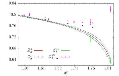
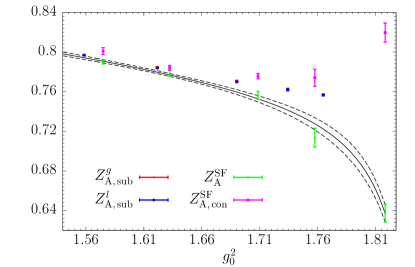
Figure 6: Comparison between different $Z_{\rm A}$ determinations for ${N_{\rm f}}=3$, obtained either from WIs in the standard SF or from universality relations in the $\chi{\rm SF}$. The $\chi{\rm SF}$ results are taken from table 7 and the effect of the perturbative one-loop improvement is shown in the right panel. The individual SF points labelled $Z_{\rm A}^{\rm SF}$ and $Z_{\rm A,con}^{\rm SF}$ are taken from ref. [22] and correspond to the definitions $Z_{\rm A,0}$ and $Z_{\rm A,0}^{\rm con}$, respectively, of that reference. The solid black line is the fit formula to $Z_{\rm A}^{\rm SF}$ also given in [22] and the dashed lines delimit the $1\sigma$ region of the fit. Note that this fit function enforces the perturbative 1-loop behaviour for $g_{0}^{2}\to 0$.

In conclusion, our final results for $Z_{\rm A,V}$ are very precise for both LCPs. Similarly to the ${N_{\rm f}}=2$ case, the results for $Z_{\rm A}$ are significantly more accurate than the standard SF determination based on Ward identities [22]. This can be appreciated in figure 6, where the results from table 7 are displayed together with the 2 alternative definitions $Z_{\rm A,0}$ and $Z_{\rm A,0}^{\rm con}$ of ref. [22].

5.3 Universality and automatic O($a$) improvement

Given our estimates for $Z_{\rm A,V}$ we can study the approach to the continuum limit of the ratio between different definitions. We begin with figure 7 where the ratios between the $g$- and $l$-definitions are considered for the $L_{1}$- and $L_{2}$-LCPs; both the results before and after perturbative improvement are shown. The conclusions are very much the same as for the ${N_{\rm f}}=2$ case. Considering the results before perturbative improvement, along both LCPs, the $g$ and $l$ definitions deviate by at most a couple of per-cent. These differences then perfectly scale with $a^{2}$ to zero as the continuum limit is approached. If perturbative improvement is implemented, these differences almost vanish even at the coarsest lattice spacings. There is no significant deviation from $a^{2}$ scaling, however, some small admixture of higher order effects cannot be excluded either.

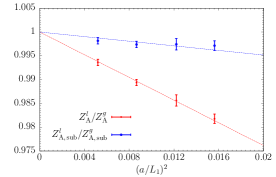
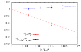
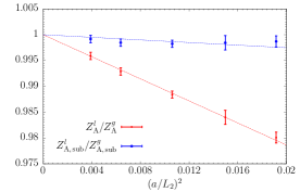
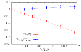
Figure 7: Continuum limit of the ratios between the $l$ and $g$ definitions of $Z_{\rm A}$ (left panels) and $Z_{\rm V}$ (right panels) for the case of ${N_{\rm f}}=3$ quark-flavours; the effect of subtracting the lattice artefacts from the $Z$-factors to O($g_{0}^{2}$) is also shown. The upper panels show the $L_{1}$-LCP results while the lower ones show those of the $L_{2}$-LCP. In all cases, the dashed lines correspond to linear fits to the data constrained to extrapolate to 1 for $a/L_{1,2}=0$. Note that the (tiny) effect of the statistical correlation between numerator and denominator has been neglected in these ratios.

It is also interesting to consider the continuum limit of the ratio between the definitions belonging to different LCPs i.e. the $L_{1}$- and $L_{2}$-LCP. An example of such a ratio is shown in figure 8. Also in this case, the continuum scaling of this ratio is the one expected, and the initial difference is at the 2 per cent level. Apart from providing an important check of universality and automatic O($a$) improvement, these results show that considering one definition or the other for the renormalization of matrix elements of the axial and vector currents, will only introduce small O($a^{2}$) differences over the whole range of lattice spacings covered.

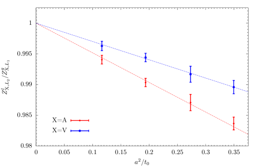
Figure 8: Continuum limit of the ratio between the $Z^{l}_{{\rm X},\,L_{2}}$ definitions, X=A,V, corresponding to the $L_{2}$-LCP, and the $Z^{g}_{{\rm X},\,L_{1}}$ definitions corresponding to the $L_{1}$-LCP. The dashed lines correspond to linear fits to the data constrained to extrapolate to 1 for $a^{2}/t_{0}=0$.

Finally, we look at ratios between $\chi{\rm SF}$ and standard SF determinations. Towards the continuum limit these should also scale like $1+{\rm O}(a^{2})$, if the SF determinations are O($a$) improved. In figure 9 we show the continuum limit of the ratios between the standard SF determinations of ref. [22] and the $\chi{\rm SF}$ results of table 7. We here consider both definitions of this reference, and label them as $Z_{\rm A}^{\rm SF}=Z_{\rm A,0}$ and $Z_{\rm A,\,con}^{\rm SF}=Z_{\rm A,0}^{\rm con}$, respectively (cf. [22] for the exact definitions).

As one can see in figure 9, for their preferred definition, $Z^{\rm SF}_{\rm A}$, the expected scaling is only setting in around $a^{2}/t_{0}<0.2$, where the SF and $\chi{\rm SF}$ determinations differ by a couple of per cent. At the coarsest lattice spacing, corresponding to $\beta=3.4$, the deviation from the O($a^{2}$) scaling is significant. The results for $Z_{\rm A}^{g}$ show the largest deviation from the SF determination, which is about 6%. Considering the perturbatively improved $\chi{\rm SF}$ results this difference is somewhat reduced to 4-5%, but O($a^{2}$) scaling is not observed either. If we consider instead the alternative definition, $Z^{\rm SF}_{\rm A,\,con}$, the deviation is reduced to about 2 per cent at the coarsest lattice spacing for $Z_{\rm A}^{l}$, while, remarkably, the results for $Z_{\rm A}^{g}$ and $Z^{\rm con}_{\rm A,0}$ are compatible within errors. In particular, the difference between this SF and both our $\chi{\rm SF}$ determinations is perfectly compatible with an O($a^{2}$) effect over the whole range of lattice spacings considered. While discretization effects can only be defined with respect to some reference definition, we conclude that the alternative SF definition $Z_{\rm A,\,con}^{\rm SF}$ is, within errors, perfectly scaling with $a^{2}$ for $\beta\geq 3.4$ relative to all $\chi{\rm SF}$ definitions, whereas the preferred definition $Z_{\rm A}^{\rm SF}$ of ref. [22] requires much finer lattices before this expected asymptotic behaviour sets in. With hindsight, $Z_{\rm A,\,con}^{\rm SF}$ seems to be a better choice within the SF framework and also has been the preferred SF definition within the ${N_{\rm f}}=2$ setup of refs. [8, 44].

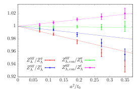
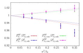
Figure 9: Continuum limit of the ratios between the ${N_{\rm f}}=3$ WI determinations of $Z_{\rm A}$ of ref. [22], and the $\chi{\rm SF}$ determinations $Z_{\rm A}^{g,l}$ (left panel) and $Z_{\rm A,\,sub}^{g,l}$ (right panel) of table 7. The $Z_{\rm A}^{\rm SF}$ results are from the fit formula provided in ref. [22], and correspond to their preferred, $Z_{\rm A,0}$, definition. The associated dashed lines (red and blue lines) are linear fits to the data with $a^{2}/t_{0}<0.2$, constrained to extrapolate to 1 for $a^{2}/t_{0}=0$. The $Z_{\rm A,\,con}^{\rm SF}$ results come instead from a fit of the results for the alternative, $Z_{\rm A,0}^{\rm con}$, definition considered in ref. [22]. The latter fit was obtained using the same fit ansatz used in ref. [22] for $Z_{\rm A,0}$. The associated dashed lines (green and magenta lines) are linear fits to all data, constrained to extrapolate to 1 for $a^{2}/t_{0}=0$.

6 Summary and conclusions

We have used a new method [20] based on the chirally rotated Schrödinger functional [14] to obtain high precision results for the normalization constants of the Noether currents corresponding to non-singlet chiral and flavour symmetries. The matrix elements of these axial and vector currents play a crucial rôle in various contexts of hadronic physics. Our method differs from the traditional Ward identity method [11, 12] in that it compares correlation functions which are related by finite chiral or flavour rotations, rather than infinitesimal ones. The major advantage compared to the Ward identity method consists in the avoidance of 3- and 4-point functions in favour of simple 2-point functions. This very significantly improves on the precision achieved in previous determinations [21, 44, 8, 22, 47]. In particular, for the case of $Z_{\rm A}$, we obtain a reduction of the error by up to an order of magnitude (cf. figure 3 and 6). The relatively poor precision obtained for $Z_{\rm A}$ with the traditional Ward identity methods [21, 44, 8, 22] (around the percent level at the coarsest lattice spacings of interest), has now become a limiting factor in several applications. For this reason, our results are in high demand and have already been used in several works [1, 23, 48]. In particular, the precise ${N_{\rm f}}=2+1$ scale setting from a linear combination of $f_{K}$ and $f_{\pi}$ in ref. [1] crucially relies on our values of $Z_{\rm A}^{l}$ in table 6 and the associated uncertainty is negligible compared to the statistical error of the bare hadronic matrix elements. In turn, the precise scale setting result of [1] is entering almost all studies done with CLS gauge configurations: in particular it has enabled the precise result for the 3-flavour QCD $\Lambda$-parameter and thus $\alpha_{s}(m_{Z})$ by the ALPHA-collaboration [49, 41, 2, 50]. Further applications of our $Z_{\rm A}$-results include the non-perturbative quark mass renormalization factor in [23] and the related determination of the light and strange quark masses [48]. Regarding the ${N_{\rm f}}=2$ case, the potential improvement of the scale setting in ref. [8] due to our $Z_{\rm A}$-results would be very significant, too. Tentative estimates anticipate a gain by a factor $3-6$ in precision, when going from the finest to the coarsest lattice spacing [51].

In order to maximize the usefulness of our results we have chosen the same actions and the same $\beta$-values for ${N_{\rm f}}=2$ and ${N_{\rm f}}=3$ lattice QCD as used by the CLS initiative [8, 10]. Hence, anyone working with CLS gauge configurations will be able to directly use our results: for ${N_{\rm f}}=2$ we recommend to use $Z_{\rm A,V,\,sub}^{l}$ from table 4, and for ${N_{\rm f}}=3$ we recommend using $Z_{\rm A,V,\,sub}^{l}$ either of table 6 or 7. Although the results for $Z_{\rm A,V,\,sub}^{l}$ are slightly less precise than those for $Z_{\rm A,V,\,sub}^{g}$, their $L/a$-interpolations turn out to be more robust. Furthermore, the effect of the perturbative subtraction of cutoff effects is rather small and only marginally significant with current errors. While the precise choice of the $\chi{\rm SF}$ results for the $Z$-factors is not crucial, it is however very important to be consistent and to not switch definitions when changing $\beta$. Only then cutoff effects are guaranteed to vanish smoothly at a rate $\propto a^{2}$.

Our determination of $Z_{\rm A,V}(\beta)$ was carried out for each $\beta$-value independently, in order to avoid adding statistical correlation between physics results at different lattice spacings. However, it is straightforward to fit our $Z$-factors to a smooth function of $\beta$ (or $g_{0}^{2}$), which interpolates to any intermediate $\beta$-value. We have included a few such fits in appendix C to our preferred definitions $Z_{\rm A,V,\,sub}^{l}$. We also include fits which incorporate the expected perturbative behaviour to 1-loop order. However, the high precision obtained in the $\beta$-range covered by the data cannot be guaranteed outside this range. If a similar precision is required at higher $\beta$, an extension of our non-perturbative determination will be required. If $t_{0}/a^{2}$ was known for higher $\beta$-values one could extend our chosen line of constant physics covering another factor of 2 or so in the lattice spacing. The required simulations of the $\chi$SF for lattice sizes up to $L/a=32$ would be feasible with current resources. Going beyond this range it may be advisable to choose a different line of constant physics from a finite volume observable, or at least estimate the errors incurred by deviating from the original choice.

In applications to hadronic physics one would also like to control the O($a$) effects cancelled by the counterterms to the currents. Close to the chiral limit, one essentially requires the counterterm coefficients $c_{\rm A,V}$ [26, 27]. We emphasize that our method of determining the $Z$-factors does not rely on any assumptions about these counterterms and can therefore be combined with results for $c_{\rm A,V}$ from other studies, e.g. [52, 47]. The same remark applies to the $b$-coefficients multiplying O($am$) counterterms, which have recently been determined for the vector current in ref. [53].

Looking beyond direct applications of our results in the CLS context, it is quite obvious that the precision gains of this method are generic and could be implemented with any other choice of Wilson type fermions. One would need to implement the $\chi$SF boundary conditions following ref. [14], as well as the $\chi$SF correlation functions [20]. We also note that the computer resources required are rather modest: in fact our largest lattice size was $16^{4}$; indeed, the main work for the present results went into painstakingly following lines of constant physics and the determination of the corresponding uncertainties and their propagation to the $Z$-factors. We have reported many technical details in the hope that any further applications of the method will be able to benefit from our experience. One possible improvement we did not explore was to measure the derivatives (3.29,3.30) by computing the corresponding operator insertions into the correlation functions directly on the tuned ensembles; this was done e.g. in refs. [1, 2] for the PCAC mass, $t_{0}$, and other observables, and this would certainly allow one to further improve on the precision, as no assumptions on the derivatives need to be made.

Possible future applications of the $\chi$SF include the determination of the ratio between pseudo-scalar and scalar renormalization constants, $Z_{\rm P}/Z_{\rm S}$. Advantages of the $\chi$SF are also expected for scale-dependent problems, such as the renormalization of 4-quark operators, where the contamination by O($a$) effects could be significantly reduced by the mechanism of automatic O($a$) improvement [19]. Finally the $\chi$SF offers new methods for the determination of O($a$) improvement coefficients, which we hope to explore in the future.

7 Acknowledgments

We would like to thank Rainer Sommer and Stefano Lottini for useful discussions, and Patrick Fritzsch, Tim Harris, and Alberto Ramos for helpful comments on the analysis of the data. We are moreover thankful to the computer centers at ICHEC, LRZ (project id pr84mi), and DESY-Zeuthen for the allocated computer resources and support. The code we used for the simulations is based on the openQCD package developed at CERN [38].

Appendix A Simulation parameters and results

$L/a$	$\beta$	$\kappa$	$z_{f}$	$mL\times 10^{3}$	$g_{\rm A}^{ud}(L/2)\times 10^{3}$	$P_{\rm Q}$	$N_{\rm ms}$
$8$	$5.2$	$0.1356450$	$1.28300$	$-0.8(1.4)$	$-2.9(2.2)$	$99.8\%$	$8002$
$8$	$5.3$	$0.1361712$	$1.28680$	$\phantom{-}0.9(1.0)$	$\phantom{-}1.0(1.5)$	$99.9\%$	$12002$
$10$	$5.3$	$0.1362811$	$1.30900$	$-3.1(1.7)$	$\phantom{-}6.6(2.3)$	$98.6\%$	$4004$
$12$	$5.3$	$0.1363310$	$1.32280$	$\phantom{-}0.1(2.3)$	$\phantom{-}7.5(2.8)$	$93.8\%$	$2403$
$12$	$5.5$	$0.1367093$	$1.31120$	$\phantom{-}1.8(1.6)$	$-2.0(1.9)$	$99.4\%$	$2403$
$16$	$5.7$	$0.1367058$	$1.30600$	$-0.2(1.4)$	$\phantom{-}1.4(1.6)$	$100\%$	$1803$

Table 8: Parameters of the ${N_{\rm f}}=2$ ensembles and corresponding results for $mL$ and $g_{\rm A}^{ud}(L/2)$. The total number of measurements we collected is given by $N_{\rm ms}$; these are spaced by 10 MDUs. In the table we also give the percentage $P_{Q}$ of gauge fields with $Q=0$.

$L/a$	$\beta$	$\kappa$	$z_{f}$	$mL\times 10^{3}$	$g_{\rm A}^{ud}(L/2)\times 10^{3}$	$P_{Q}$	$N_{\rm ms}$
$6$	$3.40$	$0.1364794$	$1.33331$	$-0.19(99)$	$\phantom{-}3.1(1.6)$	99.9%	31208
$8$	$3.40$	$0.1366405$	$1.37100$	$-0.3(1.0)$	$-1.4(1.6)$	98.4%	18620
$10$	$3.40$	$0.1367529$	$1.40741$	$-2.0(1.8)$	$-2.7(2.5)$	92.3%	14416
$12$	$3.40$	$0.1368158$	$1.43650$	$\phantom{-}0.5(2.0)$	$-2.0(2.8)$	72.9%	21685
$6$	$3.46$	$0.1367283$	$1.33580$	$\phantom{-}0.06(84)$	$-0.9(1.5)$	99.95%	31208
$8$	$3.46$	$0.1368457$	$1.36250$	$\phantom{-}1.2(1.5)$	$\phantom{-}0.2(2.1)$	99.4%	8002
$10$	$3.46$	$0.1369430$	$1.39170$	$-3.7(1.5)$	$\phantom{-}3.4(2.1)$	96.1%	12441
$12$	$3.46$	$0.1369731$	$1.40600$	$\phantom{-}2.9(2.2)$	$-0.5(2.8)$	83.1%	5109
$8$	$3.55$	$0.1370247$	$1.35500$	$-0.3(1.3)$	$-0.4(1.8)$	99.85%	8002
$10$	$3.55$	$0.1370827$	$1.37200$	$-0.45(95)$	$\phantom{-}0.7(1.3)$	99.1%	7712
$12$	$3.55$	$0.1371100$	$1.38320$	$-0.6(1.6)$	$\phantom{-}2.0(2.1)$	96.4%	4004
$16$	$3.55$	$0.1371487$	$1.40530$	$-0.3(1.7)$	$-3.3(1.9)$	71.2%	6404
$8$	$3.70$	$0.1370673$	$1.34250$	$-0.55(99)$	$\phantom{-}0.8(1.5)$	100%	8002
$10$	$3.70$	$0.1370938$	$1.35164$	$\phantom{-}0.9(1.6)$	$-3.9(2.4)$	99.4%	3208
$12$	$3.70$	$0.1371160$	$1.35860$	$-2.2(1.3)$	$\phantom{-}0.0(2.0)$	99.9%	8000
$16$	$3.70$	$0.1371370$	$1.36790$	$-1.0(1.2)$	$\phantom{-}0.7(1.3)$	91.9%	4004
$16$	$3.85$	$0.1369595$	$1.34540$	$\phantom{-}0.6(1.0)$	$\phantom{-}1.4(1.1)$	99.1%	4354

Table 9: Parameters of the ${N_{\rm f}}=3$ ensembles and corresponding results for $mL$ and $g_{\rm A}^{ud}(L/2)$. The total number of measurements we collected is given by $N_{\rm ms}$; these are spaced by 10 MDUs. In the table we also give the percentage $P_{Q}$ of gauge fields with $Q=0$.

$L/a$	$\beta$	$\kappa$	$z_{f}$	$Z_{\rm A}^{g}$	$Z_{\rm A}^{l}$	$Z_{\rm V}^{g}$	$Z_{\rm V}^{l}$
$8$	$5.2$	$0.1356450$	$1.28300$	$0.78022(24)(44)(22)$	$0.76944(19)(43)(82)$	$0.746732(128)(443)(94)$	$0.73849(21)(46)(83)$
$8$	$5.3$	$0.1361712$	$1.28680$	$0.78767(16)(34)(15)$	$0.77754(13)(33)(55)$	$0.756611(93)(346)(62)$	$0.74806(14)(36)(55)$
$10$	$5.3$	$0.1362811$	$1.30900$	$0.78204(22)(76)(36)$	$0.77505(18)(74)(135)$	$0.75000(12)(77)(15)$	$0.74539(19)(80)(136)$
$12$	$5.3$	$0.1363310$	$1.32280$	$0.77957(30)(55)(33)$	$0.77331(22)(54)(124)$	$0.74639(15)(56)(14)$	$0.74327(25)(58)(126)$
$12$	$5.5$	$0.1367093$	$1.31120$	$0.79450(18)(57)(24)(111)$	$0.78955(13)(56)(88)(79)$	$0.76634(12)(58)(10)(131)$	$0.76253(15)(60)(89)(86)$
$16$	$5.7$	$0.1367058$	$1.30600$	$0.80526(12)(35)(16)(88)$	$0.802768(86)(345)(587)(624)$	$0.779955(88)(358)(67)(1039)$	$0.778014(99)(371)(595)(676)$

Table 10: Renormalization constants $Z_{\rm A,V}^{g,l}$ for the different ${N_{\rm f}}=2$ ensembles. The four errors refer to (cf. appendix B): statistical, systematic coming from the uncertainty on $am_{\rm cr}$ ($\Delta_{m_{0}}Z_{\rm A,V}$), systematic coming from the uncertainty on $z^{*}_{f}$ ($\Delta_{z_{f}}Z_{\rm A,V}$), and systematic coming from maintaining the condition (4.33) ($\Delta_{x}Z_{\rm A,V}$); the latter is only relevant for the last two ensembles.

$L/a$	$\beta$	$\kappa$	$z_{f}$	$Z_{\rm A,\,sub}^{g}$	$Z_{\rm A,\,sub}^{l}$	$Z_{\rm V,\,sub}^{g}$	$Z_{\rm V,\,sub}^{l}$
$8$	$5.2$	$0.1356450$	$1.28300$	$0.77262(24)(44)(22)$	$0.76963(19)(43)(82)$	$0.739864(127)(443)(94)$	$0.73890(21)(46)(83)$
$8$	$5.3$	$0.1361712$	$1.28680$	$0.78016(15)(34)(15)$	$0.77772(13)(33)(55)$	$0.749804(92)(346)(62)$	$0.74846(14)(36)(55)$
$10$	$5.3$	$0.1362811$	$1.30900$	$0.77738(22)(76)(36)$	$0.77519(18)(74)(135)$	$0.74570(12)(77)(15)$	$0.74562(19)(80)(136)$
$12$	$5.3$	$0.1363310$	$1.32280$	$0.77638(30)(55)(33)$	$0.77342(22)(54)(124)$	$0.74343(15)(56)(14)$	$0.74342(25)(58)(126)$
$12$	$5.5$	$0.1367093$	$1.31120$	$0.79138(18)(57)(24)(62)$	$0.78965(13)(56)(88)(80)$	$0.76343(12)(58)(10)(88)$	$0.76268(15)(60)(89)(89)$
$16$	$5.7$	$0.1367058$	$1.30600$	$0.80358(12)(35)(16)(49)$	$0.802833(86)(345)(587)(631)$	$0.778359(87)(358)(67)(693)$	$0.778097(99)(371)(595)(699)$

Table 11: Renormalization constants $Z_{\rm A,V,\,sub}^{g,l}$ for the different ${N_{\rm f}}=2$ ensembles. Lattice artefacts have been subtracted at O($g_{0}^{2}$) in perturbation theory. The four errors refer to (cf. appendix B): statistical, systematic coming from the uncertainty on $am_{\rm cr}$ $(\Delta_{m_{0}}Z_{\rm A,V})$, systematic coming from the uncertainty on $z^{*}_{f}$ $(\Delta_{z_{f}}Z_{\rm A,V})$, and systematic coming from maintaining the condition (4.33) ($\Delta_{x}Z_{\rm A,V}$); the latter is only relevant for the last two ensembles. Comparing with the results of table 11, only the mean values, statistical errors, and errors associated with maintaining the condition (4.33), are different. The mean values and corresponding statistical errors can be obtained from those of table 11 through eq. (3.26). For determining the systematic errors associated with the uncertainty on $am_{\rm cr}$ and $z^{*}_{f}$ we use the same estimates for the relevant derivatives as for the results in table 11: we thus obtain the same values. The systematic errors associated with maintaining the condition (4.33), instead, involve different derivatives for the data in table 11 and the perturbatively improved ones (cf. appendix B).

$L/a$	$\beta$	$\kappa$	$z_{f}$	$Z_{\rm A}^{g}$	$Z_{\rm A}^{l}$	$Z_{\rm V}^{g}$	$Z_{\rm V}^{l}$
$6$	$3.40$	$0.1364794$	$1.33331$	$0.77905(18)(38)(15)$	$0.75899(15)(29)(69)$	$0.74294(11)(32)(11)$	$0.72534(18)(33)(71)$
$8$	$3.40$	$0.1366405$	$1.37100$	$0.768471(184)(286)(98)$	$0.75446(14)(32)(58)$	$0.729230(84)(253)(35)$	$0.71940(15)(37)(58)$
$10$	$3.40$	$0.1367529$	$1.40741$	$0.76315(28)(68)(20)$	$0.75190(20)(77)(120)$	$0.721224(93)(603)(72)$	$0.71552(27)(88)(119)$
$12$	$3.40$	$0.1368158$	$1.43650$	$0.76227(41)(54)(18)$	$0.75037(22)(61)(105)$	$0.716639(76)(478)(63)$	$0.71220(33)(70)(104)$
$6$	$3.46$	$0.1367283$	$1.33580$	$0.784318(159)(294)(57)$	$0.76501(13)(22)(44)$	$0.750160(100)(263)(46)$	$0.73259(15)(26)(44)$
$8$	$3.46$	$0.1368457$	$1.36250$	$0.77445(25)(46)(17)$	$0.76154(21)(60)(76)$	$0.738058(142)(416)(69)$	$0.72806(22)(60)(70)$
$10$	$3.46$	$0.1369430$	$1.39170$	$0.76852(21)(75)(27)$	$0.75933(18)(98)(126)$	$0.730708(84)(677)(114)$	$0.72552(21)(97)(116)$
$12$	$3.46$	$0.1369731$	$1.40600$	$0.76711(41)(81)(27)$	$0.75760(29)(105)(123)$	$0.72743(14)(72)(11)$	$0.72293(27)(104)(113)$
$8$	$3.55$	$0.1370247$	$1.35500$	$0.78311(20)(35)(12)$	$0.77108(16)(31)(46)$	$0.749621(124)(301)(68)$	$0.73993(17)(35)(46)$
$10$	$3.55$	$0.1370827$	$1.37200$	$0.77803(13)(29)(10)$	$0.76936(10)(26)(38)$	$0.743999(68)(249)(56)$	$0.73813(11)(29)(38)$
$12$	$3.55$	$0.1371100$	$1.38320$	$0.77595(25)(45)(17)$	$0.76786(21)(40)(64)$	$0.740868(125)(393)(94)$	$0.73692(17)(46)(65)$
$16$	$3.55$	$0.1371487$	$1.40530$	$0.77378(42)(47)(19)$	$0.76676(28)(41)(69)$	$0.73723(10)(40)(10)$	$0.73456(20)(47)(70)$
$8$	$3.70$	$0.1370673$	$1.34250$	$0.796626(144)(279)(61)$	$0.78571(12)(25)(38)$	$0.766997(103)(304)(62)$	$0.75716(12)(27)(38)$
$10$	$3.70$	$0.1370938$	$1.35164$	$0.79223(18)(44)(11)$	$0.78454(16)(39)(71)$	$0.76247(12)(48)(12)$	$0.75626(18)(43)(71)$
$12$	$3.70$	$0.1371160$	$1.35860$	$0.789547(139)(539)(96)$	$0.78386(11)(47)(60)$	$0.759810(87)(588)(98)$	$0.75576(13)(53)(61)$
$16$	$3.70$	$0.1371370$	$1.36790$	$0.787298(140)(372)(70)$	$0.78283(15)(33)(44)$	$0.757196(76)(405)(71)$	$0.754818(99)(363)(440)$
$16$	$3.85$	$0.1369595$	$1.34540$	$0.799848(82)(294)(62)$	$0.796571(88)(259)(386)$	$0.773042(58)(321)(63)$	$0.770607(70)(287)(387)$

Table 12: Renormalization constants $Z_{\rm A,V}^{g,l}$ for the different ${N_{\rm f}}=3$ ensembles. The three errors refer to (cf. appendix B): statistical, systematic coming from the uncertainty on $am_{\rm cr}$ $(\Delta_{m_{0}}Z_{\rm A,V})$, and systematic coming from the uncertainty on $z^{*}_{f}$ $(\Delta_{z_{f}}Z_{\rm A,V})$. The corresponding results with the O($g_{0}^{2}$) lattice artefacts subtracted are obtained from those above by applying eq. (3.26) to the mean values and corresponding statistical errors. The systematic uncertainties are instead left unchanged (cf. table 11).

Appendix B Error propagation, systematic error estimates and comparison with perturbation theory

In this appendix we describe in some detail the elements required to carry out the steps 2,3 and 4 sketched in subsection 3.6, for the propagation of uncertainties. We first report on the numerical estimates of the various derivatives (steps 2,3) for both ${N_{\rm f}}=2$ and ${N_{\rm f}}=3$. These estimates are obtained on smaller lattices $L/a=8$ and $L/a=6,8$ respectively, and then used for all lattice sizes. We therefore also summarize the expected scaling with $L/a$ of these derivatives and confirm this to first non-trivial order in perturbation theory. Finally, the interpolation of the $Z$-factors in $L/a$ (step 4, where necessary) is discussed, first for ${N_{\rm f}}=2$, where this step is almost avoidable, and then for ${N_{\rm f}}=3$, where interpolations are necessary at most $\beta$-values, thus requiring a more thorough analysis.

B.1 Estimating the derivatives: ${N_{\rm f}}=2$

As described in section 3.6, to estimate the uncertainty in $Z_{\rm A,V}$ originating from those of $am_{\rm cr}$ and $z_{f}^{*}$, we require the derivatives (3.29) and (3.30). We estimated these through dedicated simulations at $L/a=8$ and $\beta=5.2$, measuring the relevant quantities for several different values of $\kappa$ ($z_{f}$) at fixed $z_{f}$ ($\kappa$), straddling the tuned values given in table 8. The results we obtained for the derivatives (3.29) are:

$${\partial mL\over\partial m_{0}L} =1.251(68), {\partial mL\over\partial z_{f}} =0.048(73),$$

$${\partial g^{ud}_{\rm A}\over\partial m_{0}L} =-2.719(96), {\partial g^{ud}_{\rm A}\over\partial z_{f}} =-2.39(10).$$ (B.37)

We observe that the $z_{f}$-derivative of $mL$ vanishes within an uncertainty much smaller than the values of the other derivatives, so that we may safely set it to zero. These results were then used for all other ensembles and lattice sizes listed in table 8. The uncertainty in the tuning of $mL$ and $g_{\rm A}^{ud}(L/2)$ is thus converted to one in $m_{\rm cr}L$ and $z_{f}^{*}$. Specifically, one has that,

$$\Bigg{(}\begin{array}[]{c}\Delta(m_{\rm cr}L)\\ \Delta z_{f}^{*}\end{array}\Bigg{)}=A^{-1}\Bigg{(}\begin{array}[]{c}\Delta(mL)\\ \Delta g^{ud}_{\rm A}\end{array}\Bigg{)}\quad\text{where}\quad A=\Bigg{(}\begin{array}[]{cc}{\partial mL\over\partial m_{0}L}&{\partial mL\over\partial z_{f}}\\ {\partial g^{ud}_{\rm A}\over\partial m_{0}L}&{\partial g^{ud}_{\rm A}\over\partial z_{f}}\end{array}\Bigg{)},$$ (B.38)

and $\Delta(mL)$, $\Delta g_{\rm A}^{ud}$, $\Delta(m_{\rm cr}L)$ and $\Delta z_{f}^{*}$, are the uncertainties in $mL$, $g_{\rm A}^{ud}(L/2)$, $m_{\rm cr}L$ and $z_{f}^{*}$, respectively. For the uncertainties $\Delta(mL)$ and $\Delta g_{\rm A}^{ud}$ we took the (absolute) values of $mL$ and $g_{\rm A}^{ud}(L/2)$ measured on the given ensemble (cf. table 8), plus 2 times the corresponding statistical errors. The corresponding systematic errors on the $Z$-factors can then be estimated as,

$$(\Delta_{m_{0}}Z_{{\rm X}})^{2}+(\Delta_{z_{f}}Z_{{\rm X}})^{2}=\bigg{(}{\partial Z_{\rm X}\over\partial m_{0}L}\bigg{)}^{2}(\Delta m_{\rm cr}L)^{2}+\bigg{(}{\partial Z_{\rm X}\over\partial z_{f}}\bigg{)}^{2}(\Delta z_{f}^{*})^{2},\quad{\rm X=A,V}.$$ (B.39)

Through the very same simulations used to determine the derivatives (B.37) we obtained,

$${\partial Z_{\rm A}^{g}\over\partial m_{0}L} =0.126(11), {\partial Z_{\rm A}^{l}\over\partial m_{0}L} =-0.1266(88),$$

$${\partial Z_{\rm V}^{g}\over\partial m_{0}L} =0.1376(60), {\partial Z_{\rm V}^{l}\over\partial m_{0}L} =-0.1356(98),$$ (B.40)

and

$${\partial Z_{\rm A}^{g}\over\partial z_{f}} =-0.011(12), {\partial Z_{\rm A}^{l}\over\partial z_{f}} =-0.1092(93),$$

$${\partial Z_{\rm V}^{g}\over\partial z_{f}} =-0.0017(65), {\partial Z_{\rm V}^{l}\over\partial z_{f}} =-0.108(11).$$ (B.41)

We then used these values at all other $L/a$- and $\beta$-values of table 8. More precisely, we propagated the errors according to eq. (B.39) using the measured absolute mean values to which we added twice the statistical errors. Taking these results at the coarsest available lattice spacing is a conservative choice which should be safe, also given that some favourable expected scaling of the derivative towards larger $L/a$ (s. below) is not taken advantage of. Complementary information obtained during the tuning runs for finding $m_{\rm cr}$ and $z_{f}^{*}$, further corroborates this assumption. Looking at eqs. (B.40,B.41) it is clear that the $l$-definitions have in general larger systematic uncertainties due to their larger sensitivity to $z_{f}$. This is then reflected in the $Z$-factors in tables 11 and 11 where the uncertainties are listed separately.

B.2 Estimating the derivatives: ${N_{\rm f}}=3$

For ${N_{\rm f}}=3$ we proceeded in very much the same way, except that we carried out a more complete study of $L/a=8$ lattices at all $\beta$-values, except $\beta=3.85$, and also included additional $L/a=6$ lattices at $\beta=3.4$ and $3.46$. As before for the derivatives (3.29) we used their mean values and set ${\rm d}mL/{\rm d}z_{f}=0$, while for the derivatives (3.30) we considered their (absolute) mean values plus twice their statistical errors. However, here we did this separately for all $\beta$-values, with $\beta=3.7$ results also applied at $\beta=3.85$. Table 12 contains the results for $Z_{\rm A,V}^{g,l}$ for all ensembles of table 9, including the different estimated uncertainties. As with ${N_{\rm f}}=2$, the soundness of our assumption is supported by experience gained during the tuning runs to find $m_{\rm cr}$ and $z_{f}^{*}$.

B.3 Expected scaling with $L/a$ and perturbative calculations

B.3.1 Expected $L/a$-scaling

Using general arguments based on the Symanzik expansion and $P_{5}$ parity [20] one may obtain the expected scaling with the lattice spacing $a$ of the derivatives of the PCAC mass and $g_{\rm A}^{ud}$ with respect to $m_{0}$ and $z_{f}$,

$$\dfrac{\partial g_{\rm A}^{ud}}{\partial z_{f}}={\rm O}(1),\qquad\dfrac{\partial g_{\rm A}^{ud}}{\partial m_{0}L}={\rm O}(1),$$ (B.42)

and

$$\dfrac{\partial mL}{\partial m_{0}L}={\rm O}(1),\qquad\dfrac{\partial mL}{\partial z_{f}}={\rm O}(a^{2}).$$ (B.43)

To explain how one arrives at these scaling properties we go through the example of the PCAC mass:

$$\dfrac{\partial mL}{\partial z_{f}}=L\dfrac{\partial}{\partial z_{f}}\left(\dfrac{\tilde{\partial}_{0}g_{\rm A}^{ud}}{2g_{\rm P}^{ud}}\right)=L\left(m^{\prime}-m\right)\times\dfrac{g_{{\rm P};z_{f}}^{ud}}{g_{\rm P}^{ud}},$$ (B.44)

where we have introduced the modified PCAC mass $m^{\prime}$ through the equation

$$\tilde{\partial}_{0}g_{{\rm A};z_{f}}^{ud}=2m^{\prime}g_{{\rm P};z_{f}}^{ud},$$ (B.45)

and the notation $;z_{f}$ indicates differentiation with respect to $z_{f}$ [20]. The crucial point to note is that this differentiation merely modifies the fields at the time boundaries and thus produces a different matrix element for the PCAC relation and hence the modified PCAC mass $m^{\prime}$. Since the difference $m^{\prime}-m$ between two PCAC masses is of O($a$) in general, and the $z_{f}$-derivative of the $P_{5}$-even correlation function $g_{\rm P}^{ud}$ is $P_{5}$-odd and thus of O($a$), we arrive at O($a^{2}$) for the complete expression. It is re-assuring to see that this derivative is indeed found to be small in the simulations.

Similar arguments lead to

$$\dfrac{\partial Z_{\rm A,V}^{g,l}}{\partial m_{0}L}={\rm O}(a),\qquad\dfrac{\partial Z_{\rm A,V}^{g,l}}{\partial z_{f}}={\rm O}(a),$$ (B.46)

where the derivatives are taken at fixed $\beta,z_{f}$ and $\beta,am_{0}$, respectively.

B.3.2 Comparison with perturbation theory

Perturbation theory confirms all of these expected scaling properties. The derivatives (3.29) have only been considered to tree-level, which gives,

$${\partial mL\over\partial m_{0}L} =1+{\rm O}(g_{0}^{2}), {\partial mL\over\partial z_{f}} ={\rm O}(g_{0}^{2}),$$

$${\partial g^{ud}_{\rm A}\over\partial m_{0}L} =-3+{\rm O}(g_{0}^{2}), {\partial g^{ud}_{\rm A}\over\partial z_{f}} =-6+{\rm O}(g_{0}^{2}).$$ (B.47)

For the mass sensitivity of the axial current we have, to one-loop order,

$$\dfrac{\partial Z_{\rm A}^{g}}{\partial m_{0}L} \approx \dfrac{a}{L}\times\begin{cases}1-0.47\times g_{0}^{2}+\ldots&\text{(Wilson action)},\cr 1-0.43\times g_{0}^{2}+\ldots&\text{(LW action)},\end{cases}$$ (B.48)

$$\dfrac{\partial Z_{\rm A}^{l}}{\partial m_{0}L} \approx \dfrac{a}{L}\times\left(-0.16\times g_{0}^{2}+\ldots\right)\quad\text{(LW \& Wilson action)},$$ (B.49)

and, for the vector current,

$$\dfrac{\partial Z_{\rm V}^{g}}{\partial m_{0}L} \approx \dfrac{a}{L}\times\begin{cases}1-0.48\times g_{0}^{2}+\ldots&\text{(Wilson action)},\cr 1-0.44\times g_{0}^{2}+\ldots&\text{(LW action)},\end{cases}$$ (B.50)

$$\dfrac{\partial Z_{\rm V}^{l}}{\partial m_{0}L} \approx \dfrac{a}{L}\times\begin{cases}-0.20\times g_{0}^{2}+\ldots&\text{(Wilson action)},\cr-0.19\times g_{0}^{2}+\ldots&\text{(LW action)}.\end{cases}$$ (B.51)

Here, the one-loop coefficients are the values at $L/a=12$ and are stable within 3-10 per cent for the range $L/a$ from 8 to 16. Incidentally, this result resolves qualitatively a puzzle posed by the non-perturbative results, eq. (B.40), where the derivatives of the $g$- and $l$-definitions are almost the same in magnitude and opposite in sign, whereas the tree level results are 1 and 0, respectively, as first noticed in [20].

The $z_{f}$-sensitivity of the $Z$-factors is easily described: all $z_{f}$-derivatives vanish at tree level and the one-loop coefficients for the $g$-definitions are very small and vanish with a rate roughly proportional to $a^{3}$ for $Z^{g}_{\rm A,V}$ and both gauge actions. On the other hand, the $l$-definitions behave as expected (s. above): very similar numbers are obtained which are, for both gauge actions, within a few percent given by

$$\dfrac{\partial Z_{\rm A,V}^{l}}{\partial z_{f}}=-0.32\times g_{0}^{2}\dfrac{a}{L}+{\rm O}(g_{0}^{4}).$$ (B.52)

For completeness we report the perturbative results for $am_{\rm cr}$ and $z_{f}^{*}$ we obtain from the same computation. For the critical mass to order $g_{0}^{2}$, the known values [54, 55, 35, 32] (with $C_{F}=4/3$ for gauge group SU(3)),

$$am_{\rm cr}=g_{0}^{2}C_{\rm F}\times\begin{cases}-0.2025565(3),&\text{(Wilson action),}\cr-0.1509201(1),&\text{(LW action)},\end{cases}$$ (B.53)

are already reproduced to 4-5 digits on lattices with $L/a$ in the range from 8 to 16. As for $z_{f}^{*}$, we have, to order $g_{0}^{2}$ and for $a/L\rightarrow 0$,

$$z_{f}^{*}=1+g_{0}^{2}C_{\rm F}\times\begin{cases}0.16759(1),&\text{(Wilson action)},\cr 0.12923(5),&\text{(LW action)},\end{cases}$$ (B.54)

where the Wilson action result is from ref. [20], whereas the LW action value is the one of $L/a=16$ with a generous guess for the error. Also in this case the values at finite $L/a$ from 8 and 16 coincide with these numbers to 4-5 digits precision.

We observe that the quantitative comparison of non-perturbative data with bare perturbation theory to order $g_{0}^{2}$ works quite well in certain cases. For instance, for ${N_{\rm f}}=2$ at $\beta=5.2$, we compare the non-perturbative value $am_{\rm cr}=-0.3282$ to $am_{\rm cr}=-0.3116+{\rm O}(g_{0}^{4})$, and similarly for $z_{f}^{*}=1.288$ we need to compare to $z_{f}^{*}=1.258+{\rm O}(g_{0}^{4})$. Also the non-perturbative current normalization constants themselves are reproduced by one-loop perturbation theory at the 5-10 percent level (compare table 1 with tables 4 and 6, 7). On the other hand, the majority of the derivatives differ very significantly, for instance,

$$\left.\dfrac{\partial Z_{\rm A}^{g}}{\partial m_{0}L}\right|_{\beta=5.2,L/a=8}=0.126(11)\quad\text{vs.}\quad 0.057+{\rm O}(g_{0}^{4}),$$ (B.55)

is off by a factor 2, and for the $l$-definition the comparison is between $-0.127(9)$ and $-0.023$, which differs by a factor 5. For the $z_{f}$-derivatives we note that perturbation theory correctly predicts the smallness of the sensitivity in the $g$-definition. Quantitatively, the perturbative $z_{f}$-derivatives of $Z_{\rm A,V}^{l}$ at $\beta=5.2$ and $L/a=8$ are $-0.046+{\rm O}(g_{0}^{4})$, to be compared with eq. (B.41), so again we observe a difference by a factor 2.

Finally, for the interpolations in $L/a$ of the data (s. below) we are also interested in the derivatives of the $Z$-factors with respect to $x=(a/L)^{2}$ at fixed bare coupling. In perturbation theory we can obtain approximate results from table 1. Expanding

$$R_{\rm A,V}^{g,l}=1+g_{0}^{2}\left(Z_{\rm A,V}^{(1)}+k_{\rm A,V}^{g,l}\times\dfrac{a^{2}}{L^{2}}+{\rm O}(a^{3})\right)+{\rm O}(g_{0}^{4}),$$ (B.56)

the $x$-derivatives to order $g_{0}^{2}$ are approximately given by

$$\dfrac{\partial Z_{\rm A,V}^{g,l}}{\partial x}\approx g_{0}^{2}\times k_{\rm A,V}^{g,l},$$ (B.57)

provided higher order cutoff effects are small. We find that this is quite well satisfied, with very similar coefficients for both Wilson and LW actions, given approximately by

$$k_{\rm A}^{g}\approx 0.45,\qquad k_{\rm V}^{g}\approx 0.43,$$ (B.58)

whereas $k_{\rm A,V}^{l}$ are ca. 20 to 30 times smaller in magnitude, for axial and vector cases, respectively, and come with the opposite sign. Comparing this with the $\beta=5.3$ non-perturbative data in eqs. (B.59) we see again that for the $g$-definitions these derivatives are reproduced by perturbation theory up to a factor 2, while for the $l$-definitions, perturbation theory to O($g_{0}^{2}$) is clearly missing the bulk of the effect. While, as expected, the non-perturbative derivatives are smaller than for the $g$-definitions, it seems that the smallness of the O($g_{0}^{2}$) term is an accident and higher orders are dominating at these values of $\beta$.

To conclude this comparison, perturbation theory often gives valuable qualitative information and may provide reasonable starting values for the tuning of $am_{0}$ and $z_{f}$. However, quantitatively, the agreement with non-perturbative data at lattice spacings of interest for hadronic physics hugely varies for different observables. Hence, the main practical use of perturbation theory consists in the perturbative subtraction of cutoff effects. Here, even a qualitative agreement, which may be quantitatively off by a factor 2, still means a welcome reduction of cutoff effects by 50 percent, and our data analysis does indeed point to such benefits.

Given this situation, we have refrained from using perturbative data in our estimates of the derivatives, and we have decided to ignore the favourable O($a$) scaling, eq. (B.46), when applying the results obtained at $L/a=8$ at all other $L/a$-values, too. In this respect, the tuning runs for $am_{0}$ and $z_{f}$, both for ${N_{\rm f}}=2$ and ${N_{\rm f}}=3$, provided some consistency checks which make us confident that the chosen procedure is indeed sound and rather conservative.

B.4 Interpolation in $L/a$ for ${N_{\rm f}}=2$

Once the uncertainties associated with the conditions (2.15) have been propagated to $Z_{\rm A,V}$ at given $\beta$ and $L/a$, one needs to keep the LCP condition (4.33) and also take into account the corresponding uncertainties. The choice (4.33) is made such that the $L/a=8$ results at $\beta=5.2$ satisfy this condition by definition, while at $\beta=5.3$ we needed to interpolate the results for $L/a=8,10,12$ to the target value $(L/a)(5.3)=9.18(21)$ (cf. table 3). We have performed a simple linear interpolation in $(a/L)^{2}$ which describes the data very well, similarly to the case ${N_{\rm f}}=3$ which will be discussed in more detail below. For $\beta=5.5$ and $5.7$, the simulated $L/a$ values are, within errors, compatible with the target values in table 3. Systematic errors related to the condition (4.33) were then estimated by using the slope of the interpolation in $x=(a/L)^{2}$ at $\beta=5.3$ also for the higher $\beta$-values. Note that we interpolate results with bare parameters $am_{\rm cr}$ and $z_{f}^{*}$ tuned at the given $\beta$- and $L/a$-values. Hence the derivative defines the sensitivity to a change of the physical size of the system. This is a pure cutoff effect of O($a^{2}$) on the $Z$-factors. Since, by the choice of the variable $x$, a factor $a^{2}$ is also divided out, the $x$-derivative is expected to be of O(1) and we expect a smooth dependence of this derivative on $\beta$;this expectation is in fact confirmed by the results for ${N_{\rm f}}=3$ where the slope shows a very mild $\beta$-dependence over the whole range (cf. table 13). As we are looking at an O($a^{2}$) effect in disguise, it is no surprise that the results depend on whether or not the cutoff effects have been subtracted perturbatively.

Without perturbative subtraction we obtained the results,

$${\partial Z_{\rm A}^{g}\over\partial x} =0.946(89), {\partial Z_{\rm A}^{l}\over\partial x} =0.48(16),$$

$${\partial Z_{\rm V}^{g}\over\partial x} =1.177(77), {\partial Z_{\rm V}^{l}\over\partial x} =0.54(17),$$ (B.59)

while for the perturbatively improved ones we obtain,

$${\partial Z_{\rm A}^{g}\over\partial x} =0.447(89), {\partial Z_{\rm A}^{l}\over\partial x} =0.49(16),$$

$${\partial Z_{\rm V}^{g}\over\partial x} =0.734(77), {\partial Z_{\rm V}^{l}\over\partial x} =0.56(17).$$ (B.60)

The corresponding systematic error is then simply taken to be,

$$(\Delta_{x}Z_{{\rm X}})^{2}=\bigg{(}{\partial Z_{\rm X}\over\partial x}\bigg{)}^{2}(\Delta x)^{2},\qquad{\rm X=A,V},$$ (B.61)

which is summed in quadrature to (B.39) and the statistical error from the Monte Carlo simulations. The uncertainly $\Delta x$ was estimated as:

$$\Delta x=|x-x(\beta)|+2\,\sigma(x(\beta)),$$ (B.62)

where $x(\beta)=((a/L)(\beta))^{2}$ and $\sigma(x(\beta))$ is the associated error. As a further safeguard we took for the derivatives (B.59) and (B.60) the (absolute) mean value plus twice their statistical error. We observe that the $l$-definitions have a milder $L/a$-dependence than the $g$-based ones, unless perturbative improvement is implemented.

B.5 Interpolation in $L/a$ for ${N_{\rm f}}=3$

Once the systematic errors deriving from the tuning of $am_{0}$ and $z_{f}$ have been taken into account, the results for $Z_{\rm A,V}$ at different $L/a$ and fixed $\beta$ must be interpolated to either $(L_{1}/a)(\beta)$ or $(L_{2}/a)(\beta)$, depending on the LCP; for completeness the values of $Z_{\rm A,V}$ prior to interpolation are given in table 12. We have considered three types of interpolation in $x=(a/L)^{2}$, these are: linear using all 4 available values of $L/a$ (cf. table 5), linear using only the 3 closest $L/a$-values to the target $(L_{1,2}/a)(\beta)$, and quadratic using all 4 $L/a$-values. Given this choice, the interpolations needed for the $L_{1}$- and $L_{2}$-LCPs only differ for $\beta=3.4$, where, by definition, $L_{1}/a=8$ is exact, and in the case of linear interpolations with 3 points at $\beta=3.55$. Recall that for $\beta=3.85$ no interpolation is required, as $L_{2}/a=16$ is exact and this $\beta$-value has been excluded for the $L_{1}$-LCP.

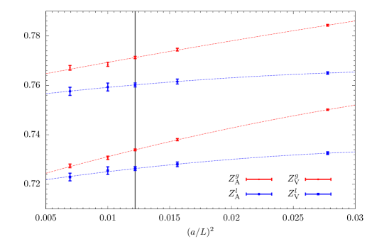
Figure 10: $L/a$-interpolations for $\beta=3.46$ and the $L_{1}$-LCP. The upper two sets of points correspond to the $Z^{g,l}_{\rm A}$ results while the lower two sets are the $Z^{g,l}_{\rm V}$ results. The dashed lines are our preferred, quadratic, fits to the data, and the interpolation points are marked by a black vertical line.

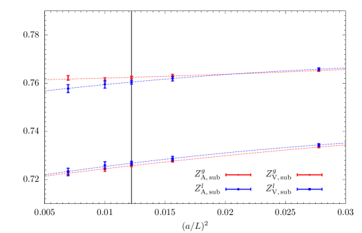
Figure 11: Same as figure 10, for the $Z$-factors with perturbative subtraction of the cutoff effects.

Starting with the $L_{1}$-LCP, the different interpolations describe the data quite well in general, particularly so for the results at the two smallest lattice spacings and for definitions based on the $l$-correlators. The most relevant exception is given indeed by the linear interpolation of $Z_{\rm V}^{g}$ at $\beta=3.46$ using all 4 values of $L/a$, for which we find a $\chi^{2}{\rm/d.o.f}\approx 2.2$. It should be noted, however, that the $\chi^{2}$-criterion does not come with the usual probability interpretation due to the errors being dominated by systematics. In any case, the interpolated values are generally compatible at the 1$\sigma$ level.

Considering the perturbatively improved data, the quality of the interpolations is generally improved, and all fits have excellent $\chi^{2}$. The beneficial effect of the perturbative improvement can be appreciated by comparing figure 10 and 11, where the $Z_{\rm A,V}$ interpolations at $\beta=3.46$ are shown for the cases before and after perturbative improvement, respectively. This example also illustrates the general feature that, before perturbative improvement, the $l$-definitions have a significantly milder $L/a$- and hence $x$-dependence. In addition, it is interesting to note that the $x$-dependence of the $Z$-factors does not change significantly over the range of $\beta$ considered, but seems in general to diminish, as expected, as $\beta\to\infty$ (cf. table 13). Based on these observations, we take as our final estimates for the $Z$-factors the results of the quadratic fits, which have the largest errors.

$\beta$	$\partial Z_{\rm A}^{g}/\partial x$	$\partial Z_{\rm A}^{l}/\partial x$	$\partial Z_{\rm V}^{g}/\partial x$	$\partial Z_{\rm V}^{l}/\partial x$
$3.46$	$0.90(11)$	$0.44(21)$	$1.25(09)$	$0.56(20)$
$3.55$	$0.69(11)$	$0.44(15)$	$1.10(08)$	$0.56(16)$
$3.70$	$0.81(10)$	$0.29(16)$	$0.87(11)$	$0.24(17)$
$\beta$	$\partial Z_{\rm A,\,sub}^{g}/\partial x$	$\partial Z_{\rm A,\,sub}^{l}/\partial x$	$\partial Z_{\rm V,\,sub}^{g}/\partial x$	$\partial Z_{\rm V,\,sub}^{l}/\partial x$
$3.46$	$0.16(11)$	$0.46(21)$	$0.58(09)$	$0.61(20)$
$3.55$	$-0.01(11)$	$0.46(15)$	$0.45(08)$	$0.60(16)$
$3.70$	$0.12(10)$	$0.31(16)$	$0.23(11)$	$0.28(17)$

Table 13: Results for $\partial Z_{\rm A,V}^{g,l}/\partial x$, where $x=(a/L)^{2}$, as a function of $\beta$ for ${N_{\rm f}}=3$ quark-flavours. The derivatives are estimated along the $L_{1}$-LCP from the linear fits using the 3 closest $L/a$-values to the target $(L_{1}/a)(\beta)$.

Regarding the $L_{2}$-LCP, the situation is more complicated due to the fact that we need to interpolate the data at the coarsest lattice spacing, $\beta=3.4$. The quality of the interpolations is still good in general, but there are a few significant exceptions. We note that all these cases involve $g$-definitions: indeed, we obtain a pretty large $\chi^{2}/$d.o.f. for the linear fits of $Z_{\rm V}^{g}$ at $\beta=3.4$ and $3.46$, around $7.8$ and $5$ respectively. Also the quadratic fit for $Z_{\rm A}^{g}$ at $\beta=3.4$ has a large $\chi^{2}{\rm/d.o.f}\approx 1.8$. While in this case, however, the results of the interpolation are compatible with those of the linear fits within less than one standard deviation, in the case of $Z_{\rm V}^{g}$ at $\beta=3.4$ the discrepancy between the linear and quadratic interpolations is close to 3 standard deviations. The situation definitely improves when the perturbatively improved data are considered. In this case, with the exception of the linear interpolations with 4 points of $Z^{g}_{\rm V,A,\,sub}$ at $\beta=3.4$, all fits have very good $\chi^{2}$, and give compatible results within one standard deviation or so. As in the case of the $L_{1}$-LCP, we take as our final estimates for $Z_{\rm A,V}$ the results of the quadratic fits, which have the best $\chi^{2}$-values and the largest errors.

Appendix C Fit formulas for $Z_{\rm A,V}(g_{0}^{2})$

In this appendix we collect some useful fit formulas for the $Z_{\rm A,V}$ results, both for ${N_{\rm f}}=2$ and ${N_{\rm f}}=3$. We will focus on the data for $Z_{\rm A,V,\,sub}^{l}$, cf. the discussion in sect. 6.

C.1 ${N_{\rm f}}=2$

For ${N_{\rm f}}=2$ the final $Z_{\rm A,V}$ results are given in table 4. Over the whole range of $\beta\in[5.2,5.7]$, the data for $Z_{\rm A,\,sub}^{l}$ is well described by a simple linear fit function,

$$Z^{l}_{\rm A,\,sub}=c_{1}+c_{2}g_{0}^{2},$$

$$c_{1,2}=\begin{pmatrix}\phantom{+}1.15183\\ -0.33176\end{pmatrix}\qquad{\rm Cov}=10^{-3}\times\begin{pmatrix}\phantom{+}0.17228874&-0.15443145\\ -0.15443145&\phantom{+}0.13858044\end{pmatrix},$$ (C.63)

which has a $\chi^{2}/{\rm d.o.f.}=0.759/2$.

Similarly, for the vector current renormalization, $Z_{\rm V,\,sub}^{l}$, a good description of the data is given by,

$$Z^{l}_{\rm V,\,sub}=c_{1}+c_{2}g_{0}^{2},$$

$$c_{1,2}=\begin{pmatrix}\phantom{+}1.18984\\ -0.39138\end{pmatrix}\qquad{\rm Cov}=10^{-3}\times\begin{pmatrix}\phantom{+}0.19505967&-0.17469696\\ -0.17469696&\phantom{+}0.15663400\end{pmatrix},$$ (C.64)

which has a $\chi^{2}/{\rm d.o.f.}=0.866/2$.

C.1.1 Matching with perturbation theory

It is also interesting to consider fit functions with the correct perturbative 1-loop behaviour for $g_{0}^{2}\to 0$ (cf. sect. 3.2). In the case of $Z_{\rm A,\,sub}^{l}$ this is possible using a 2-parameter polynomial fit,

$$Z^{l}_{\rm A,\,sub}=1-0.116458\,g_{0}^{2}+c_{1}g_{0}^{4}+c_{2}g_{0}^{6},$$

$$c_{1,2}=\begin{pmatrix}-0.015248\\ -0.049793\end{pmatrix}\qquad{\rm Cov}=10^{-3}\times\begin{pmatrix}\phantom{+}0.12545440&-0.11198363\\ -0.11198363&\phantom{+}0.10005857\end{pmatrix},$$ (C.65)

which gives a $\chi^{2}/{\rm d.o.f.}=1.519/2$. We note that the same fit ansatz was used to fit the standard SF results of ref. [8]. Similarly, for the vector current data, $Z_{\rm V,\,sub}^{l}$, we have,

$$Z^{l}_{\rm V,\,sub}=1-0.129430\,g_{0}^{2}+c_{1}g_{0}^{4}+c_{2}g_{0}^{6},$$

$$c_{1,2}=\begin{pmatrix}-0.005952\\ -0.068180\end{pmatrix}\qquad{\rm Cov}=10^{-3}\times\begin{pmatrix}\phantom{+}0.14221117&-0.12684203\\ -0.12684203&\phantom{+}0.11324469\end{pmatrix},$$ (C.66)

which gives a $\chi^{2}/{\rm d.o.f.}=1.866/2$. We stress that although the latter fit functions encode the expected asymptotic behaviour far outside the $\beta$-range covered by the data, it is not recommended to use them for $\beta$ values much outside this range. For $\beta\in[5.2,5.7]$, the two sets of fit functions agree within less than $1\sigma$ deviations.

C.2 ${N_{\rm f}}=3$

For the case ${N_{\rm f}}=3$, our final $Z_{\rm A,V}$ results are given in table 6 and 7. Having one additional $\beta$-value, it is natural to prefer an interpolation of the $L_{2}$-LCP data of table 7. The higher precision of the data compared to ${N_{\rm f}}=2$, and the availability of a fifth data point suggests to use 3-parameter fits in this case. We find that, for the whole range of $\beta\in[3.4,3.85]$, $Z^{l}_{\rm A,\,sub}$, is well described by the quadratic fit:

$$Z^{l}_{\rm A,\,sub}=c_{1}+c_{2}g_{0}^{2}+c_{3}g_{0}^{4},$$ (C.67)

with coefficients and covariance given by

$$c_{1,2,3}=\begin{pmatrix}\phantom{+}1.35510\\ -0.501106\\ \phantom{+}0.091656\end{pmatrix}\qquad{\rm Cov}=10^{-1}\times\begin{pmatrix}\phantom{+}0.229571866&-0.278151898&\phantom{+}0.084105454\\ -0.278151898&\phantom{+}0.337131945&-0.101975449\\ \phantom{+}0.084105454&-0.101975449&\phantom{+}0.030856380\end{pmatrix},$$

and $\chi^{2}/{\rm d.o.f.}=0.622/2$.

For the vector current data, $Z_{\rm V,\,sub}^{l}$, we use the same fit function,

$$Z^{l}_{\rm V,\,sub}=c_{1}+c_{2}g_{0}^{2}+c_{3}g_{0}^{4},$$ (C.68)

and obtain

$$c_{1,2,3}=\begin{pmatrix}\phantom{+}1.32353\\ -0.459016\\ \phantom{+}0.066995\end{pmatrix}\qquad{\rm Cov}=10^{-1}\times\begin{pmatrix}\phantom{+}0.247244906&-0.299424391&\phantom{+}0.090493309\\ -0.299424391&\phantom{+}0.362743281&-0.109668066\\ \phantom{+}0.090493309&-0.109668066&\phantom{+}0.033167490\end{pmatrix},$$

which gives a $\chi^{2}/{\rm d.o.f.}=1.801/2$.

C.2.1 Matching with perturbation theory

Also in this case we consider fit functions with the correct perturbative 1-loop behaviour for $g_{0}^{2}\to 0$ (cf. sect. 3.2). Applying a 3-parameter polynomial fit of the form

$$Z^{l}_{\rm A,\,sub}=1-0.090488\,g_{0}^{2}+c_{1}g_{0}^{4}+c_{2}g_{0}^{6}+c_{3}g_{0}^{8},\\$$ (C.69)

we obtain

$$c_{1,2,3}=\begin{pmatrix}\phantom{+}0.127163\\ -0.178785\\ \phantom{+}0.051814\end{pmatrix}\qquad{\rm Cov}=10^{-2}\times\begin{pmatrix}\phantom{+}0.29841165&-0.36050066&\phantom{+}0.10868891\\ -0.36050066&\phantom{+}0.43567202&-0.13140137\\ \phantom{+}0.10868891&-0.13140137&\phantom{+}0.03964605\end{pmatrix},$$

which gives a $\chi^{2}/{\rm d.o.f.}=0.403/2$. We have also tried various Padé fits e.g. of the type used in [22]. With these fits we experienced some technical problems with the bootstrap technique, when trying to determine the covariance matrix for the fit parameters. We therefore also tried the the automatic differentiation procedure of ref. [56] which completely solved this technical problem. It turns out, however, that the best fit function of this type develops a singularity at a $\beta$-value slightly above 4, and therefore does not provide a smooth interpolation to the perturbative region. Given the good quality of the linear fits we did not pursue any further non-linear options.

Regarding the vector current data, $Z_{\rm V,\,sub}^{l}$, we have,

$$Z^{l}_{\rm V,\,sub}=1-0.100567\,g_{0}^{2}+c_{1}g_{0}^{4}+c_{2}g_{0}^{6}+c_{3}g_{0}^{8},\\$$ (C.70)

with

$$c_{1,2,3}=\begin{pmatrix}\phantom{+}0.130134\\ -0.182926\\ \phantom{+}0.051526\end{pmatrix}\qquad{\rm Cov}=10^{-2}\times\begin{pmatrix}\phantom{+}0.32342173&-0.39055319&\phantom{+}0.11769835\\ -0.39055319&\phantom{+}0.47179235&-0.14223242\\ \phantom{+}0.11769835&-0.14223242&\phantom{+}0.04289459\end{pmatrix},$$

which gives a $\chi^{2}/{\rm d.o.f.}=1.443/2$.

To conclude this appendix, we emphasize again that all given fits to the data are very good if used as interpolations in the range of the non-perturbative data. Using them outside this range is at the user’s own risk, even where perturbative information is used as a constraint.

References

- [1] M. Bruno, T. Korzec, and S. Schaefer, Setting the scale for the CLS flavor ensembles, Phys. Rev. D95 (2017), no. 7 074504, [arXiv:1608.08900].
- [2] ALPHA Collaboration, M. Bruno, M. Dalla Brida, P. Fritzsch, T. Korzec, A. Ramos, S. Schaefer, H. Simma, S. Sint, and R. Sommer, QCD Coupling from a Nonperturbative Determination of the Three-Flavor Parameter, Phys. Rev. Lett. 119 (2017), no. 10 102001, [arXiv:1706.03821].
- [3] K. G. Wilson, Confinement of Quarks, Phys. Rev. D10 (1974) 2445–2459.
- [4] Hadron Spectrum Collaboration, H.-W. Lin et al., First results from 2+1 dynamical quark flavors on an anisotropic lattice: light-hadron spectroscopy and setting the strange-quark mass, Phys. Rev. D79 (2009) 034502, [arXiv:0810.3588].
- [5] PACS-CS Collaboration, S. Aoki et al., Physical Point Simulation in 2+1 Flavor Lattice QCD, Phys. Rev. D81 (2010) 074503, [arXiv:0911.2561].
- [6] W. Bietenholz et al., Tuning the strange quark mass in lattice simulations, Phys. Lett. B690 (2010) 436–441, [arXiv:1003.1114].
- [7] R. Baron et al., Light hadrons from lattice QCD with light (u,d), strange and charm dynamical quarks, JHEP 06 (2010) 111, [arXiv:1004.5284].
- [8] P. Fritzsch et al., The strange quark mass and Lambda parameter of two flavor QCD, Nucl. Phys. B865 (2012) 397–429, [arXiv:1205.5380].
- [9] S. Borsanyi et al., Ab initio calculation of the neutron-proton mass difference, Science 347 (2015) 1452–1455, [arXiv:1406.4088].
- [10] M. Bruno et al., Simulation of QCD with flavors of non-perturbatively improved Wilson fermions, JHEP 02 (2015) 043, [arXiv:1411.3982].
- [11] M. Bochicchio, L. Maiani, G. Martinelli, G. C. Rossi, and M. Testa, Chiral Symmetry on the Lattice with Wilson Fermions, Nucl. Phys. B262 (1985) 331.
- [12] M. Lüscher, S. Sint, R. Sommer, and H. Wittig, Nonperturbative determination of the axial current normalization constant in O(a) improved lattice QCD, Nucl. Phys. B491 (1997) 344–364, [hep-lat/9611015].
- [13] S. Sint, The Schrödinger functional with chirally rotated boundary conditions, PoS LAT2005 (2006) 235, [hep-lat/0511034].
- [14] S. Sint, The chirally rotated Schrödinger functional with Wilson fermions and automatic O(a) improvement, Nucl. Phys. B847 (2011) 491–531, [arXiv:1008.4857].
- [15] S. Sint and B. Leder, Testing universality and automatic O(a) improvement in massless lattice QCD with Wilson quarks, PoS LATTICE2010 (2010) 265, [arXiv:1012.2500].
- [16] J. G. Lopez, K. Jansen, D. Renner, and A. Shindler, A quenched study of the Schroedinger functional with chirally rotated boundary conditions: non-perturbative tuning, Nucl. Phys. B867 (2013) 567–608, [arXiv:1208.4591].
- [17] J. G. Lopez, K. Jansen, D. Renner, and A. Shindler, A quenched study of the Schroedinger functional with chirally rotated boundary conditions: applications, Nucl. Phys. B867 (2013) 609–635, [arXiv:1208.4661].
- [18] M. Dalla Brida and S. Sint, A dynamical study of the chirally rotated Schrödinger functional in QCD, PoS LATTICE2014 (2014) 280, [arXiv:1412.8022].
- [19] P. Vilaseca, M. Dalla Brida, and M. Papinutto, Perturbative renormalization of four-fermion operators with the chirally rotated Schrödinger functional, PoS LATTICE2015 (2016) 252.
- [20] M. Dalla Brida, S. Sint, and P. Vilaseca, The chirally rotated Schrödinger functional: theoretical expectations and perturbative tests, JHEP 08 (2016) 102, [arXiv:1603.00046].
- [21] M. Della Morte, R. Hoffmann, F. Knechtli, R. Sommer, and U. Wolff, Non-perturbative renormalization of the axial current with dynamical Wilson fermions, JHEP 0507 (2005) 007, [hep-lat/0505026].
- [22] J. Bulava, M. Della Morte, J. Heitger, and C. Wittemeier, Nonperturbative renormalization of the axial current in lattice QCD with Wilson fermions and a tree-level improved gauge action, Phys. Rev. D93 (2016), no. 11 114513, [arXiv:1604.05827].
- [23] ALPHA Collaboration, I. Campos, P. Fritzsch, C. Pena, D. Preti, A. Ramos, and A. Vladikas, Non-perturbative quark mass renormalisation and running in QCD, Eur. Phys. J. C78 (2018), no. 5 387, [arXiv:1802.05243].
- [24] M. Lüscher, R. Narayanan, P. Weisz, and U. Wolff, The Schrödinger functional: a renormalizable probe for non-Abelian gauge theories, Nucl. Phys. B384 (1992) 168–228, [hep-lat/9207009].
- [25] S. Sint, On the Schrödinger functional in QCD, Nucl. Phys. B421 (1994) 135–158, [hep-lat/9312079].
- [26] M. Lüscher, S. Sint, R. Sommer, and P. Weisz, Chiral symmetry and O(a) improvement in lattice QCD, Nucl. Phys. B478 (1996) 365–400, [hep-lat/9605038].
- [27] S. Sint and P. Weisz, Further results on O(a) improved lattice QCD to one loop order of perturbation theory, Nucl. Phys. B502 (1997) 251–268, [hep-lat/9704001].
- [28] S. Sint, One loop renormalization of the QCD Schrödinger functional, Nucl. Phys. B451 (1995) 416–444, [hep-lat/9504005].
- [29] S. Sint and R. Sommer, The running coupling from the QCD Schrödinger functional: a one loop analysis, Nucl. Phys. B465 (1996) 71–98, [hep-lat/9508012].
- [30] R. Frezzotti and G. Rossi, Chirally improving Wilson fermions. 1. O(a) improvement, JHEP 0408 (2004) 007, [hep-lat/0306014].
- [31] ALPHA Collaboration, R. Frezzotti, S. Sint, and P. Weisz, O(a) improved twisted mass lattice QCD, JHEP 07 (2001) 048, [hep-lat/0104014].
- [32] S. Aoki, R. Frezzotti, and P. Weisz, Computation of the improvement coefficient to one loop with improved gluon actions, Nucl. Phys. B540 (1999) 501–519, [hep-lat/9808007].
- [33] E. Gabrielli, G. Martinelli, C. Pittori, G. Heatlie, and C. T. Sachrajda, Renormalization of lattice two fermion operators with improved nearest neighbor action, Nucl. Phys. B362 (1991) 475–486.
- [34] M. Göckeler, R. Horsley, E.-M. Ilgenfritz, H. Oelrich, H. Perlt, P. E. L. Rakow, G. Schierholz, A. Schiller, and P. Stephenson, Perturbative renormalization of bilinear quark and gluon operators, Nucl. Phys. Proc. Suppl. 53 (1997) 896–898, [hep-lat/9608033].
- [35] S. Aoki, K.-i. Nagai, Y. Taniguchi, and A. Ukawa, Perturbative renormalization factors of bilinear quark operators for improved gluon and quark actions in lattice QCD, Phys. Rev. D58 (1998) 074505, [hep-lat/9802034].
- [36] M. Lüscher, Properties and uses of the Wilson flow in lattice QCD, JHEP 1008 (2010) 071, [arXiv:1006.4518].
- [37] M. Lüscher and S. Schaefer, Lattice QCD with open boundary conditions and twisted-mass reweighting, Comput. Phys. Commun. 184 (2013) 519–528, [arXiv:1206.2809].
- [38] openQCD: Simulation program for lattice QCD, http://luscher.web.cern.ch/luscher/openQCD/.
- [39] M. Lüscher, Step scaling and the Yang-Mills gradient flow, JHEP 06 (2014) 105, [arXiv:1404.5930].
- [40] P. Fritzsch, A. Ramos, and F. Stollenwerk, Critical slowing down and the gradient flow coupling in the Schrödinger functional, PoS Lattice2013 (2013) 461, [arXiv:1311.7304].
- [41] ALPHA Collaboration, M. Dalla Brida, P. Fritzsch, T. Korzec, A. Ramos, S. Sint, and R. Sommer, Slow running of the Gradient Flow coupling from 200 MeV to 4 GeV in QCD, Phys. Rev. D95 (2017), no. 1 014507, [arXiv:1607.06423].
- [42] S. Sint, Lattice QCD with a chiral twist, in Workshop on Perspectives in Lattice QCD Nara, Japan, October 31-November 11, 2005, 2007. [hep-lat/0702008].
- [43] A. Bode and H. Panagopoulos, The three loop beta function of QCD with the clover action, Nucl. Phys. B625 (2002) 198–210, [hep-lat/0110211].
- [44] M. Della Morte, R. Sommer, and S. Takeda, On cutoff effects in lattice QCD from short to long distances, Phys. Lett. B672 (2009) 407–412, [arXiv:0807.1120].
- [45] J. Bulava and S. Schaefer, Improvement of =3 lattice QCD with Wilson fermions and tree-level improved gauge action, Nucl. Phys. B874 (2013) 188–197, [arXiv:1304.7093].
- [46] S. Takeda, S. Aoki, and K. Ide, A perturbative determination of O() boundary improvement coefficients for the Schrödinger functional coupling at one loop with improved gauge actions, Phys. Rev. D68 (2003) 014505, [hep-lat/0304013].
- [47] J. Heitger, F. Joswig, A. Vladikas, and C. Wittemeier, Non-perturbative determination of and in lattice QCD, EPJ Web Conf. 175 (2018) 10004, [arXiv:1711.03924].
- [48] J. Koponen et al., Light and strange quark masses for simulations with Wilson fermions, in Proceedings, 36th International Symposium on Lattice Field Theory (Lattice2018): East Lansing, Michigan, USA, July 22-28, 2018, to appear in EPJ Web Conf.
- [49] ALPHA Collaboration, M. Dalla Brida, P. Fritzsch, T. Korzec, A. Ramos, S. Sint, and R. Sommer, Determination of the QCD -parameter and the accuracy of perturbation theory at high energies, Phys. Rev. Lett. 117 (2016), no. 18 182001, [arXiv:1604.06193].
- [50] ALPHA Collaboration, M. Dalla Brida, P. Fritzsch, T. Korzec, A. Ramos, S. Sint, and R. Sommer, A non-perturbative exploration of the high energy regime in QCD, Eur. Phys. J. C78 (2018), no. 5 372, [arXiv:1803.10230].
- [51] S. Lottini, private communication (2014).
- [52] ALPHA Collaboration, J. Bulava, M. Della Morte, J. Heitger, and C. Wittemeier, Non-perturbative improvement of the axial current in =3 lattice QCD with Wilson fermions and tree-level improved gauge action, Nucl. Phys. B896 (2015) 555–568, [arXiv:1502.04999].
- [53] P. Fritzsch, Mass-improvement of the vector current in three-flavor QCD, JHEP 06 (2018) 015, [arXiv:1805.07401].
- [54] R. Wohlert, Improved continuum limit lattice action for quarks, DESY-87-069, unpublished.
- [55] M. Lüscher and P. Weisz, O(a) improvement of the axial current in lattice QCD to one loop order of perturbation theory, Nucl. Phys. B479 (1996) 429–458, [hep-lat/9606016].
- [56] A. Ramos, Automatic differentiation for error analysis of Monte Carlo data, arXiv:1809.01289.