Recent progress in the partial-wave analysis of the diffractively produced $\pi^{-}\pi^{+}\pi^{-}$ final state at Compass

Abstract

The Compass spectrometer at CERN has collected a large data set for diffractive three-pion production of $46\times 10^{6}$ exclusive events. Based on previous conventional Partial-Wave Analyses (PWA), we performed a “freed-isobar PWA” on the same data, removing model assumptions on the dynamic isobar amplitudes for dominating waves. In this analysis, we encountered continuous mathematical ambiguities, which we were able to identify and resolve. This analysis gives an unprecedented insight in the interplay of $2\pi$ and $3\pi$ dynamics in the process. As an example we show results for a spin-exotic wave $J^{PC}_{X^{-}}=1^{-+}$ wave.

1 Diffractive $\mathbf{3\pi}$ production at Compass

In this work, we perform a Partial-Wave Analysis (PWA) of the diffractive process

$$\pi_{\text{beam}}^{-}+p_{\text{target}}\to X^{-}+p_{\text{recoil}}\to\pi^{-}\pi^{+}\pi^{-}+p_{\text{recoil}}$$

measured by the Compass experiment at CERN using an $190\,\text{GeV}/c$ negative hadron beam—consisting to 97% of negative pions—impinging on a liquid hydrogen target. For this process the Compass collaboration has recorded a very large data set of $46\times 10^{6}$ exclusive events, performed a very detailed PWA on this data using a set of 88 partial waves massIndepPaper , and extracted resonance masses and widths of eleven intermediate isovector resonances $X^{-}$ massDepPaper .

2 Freed-isobar PWA

The PWA preformed in Ref. massIndepPaper relies on the isobar model, in which the decay of the intermediate state $X^{-}$ into the $3\pi$ final state is modeled as a sequence of two-particle decays involving a second intermediate state $\xi^{\,0}$, the isobar:

$$X^{-}\to\xi^{\,0}+\pi^{-}_{\text{bachelor}}\to\pi^{-}\pi^{+}\pi^{-};$$

the best known examples for such isobars are the $\rho(770)$, $f_{0}(980)$, and $f_{2}(1270)$ resonances. In the conventional approach, the dynamic amplitudes of these isobar resonances $\Delta_{\xi^{\,0}}\big{(}m_{\xi^{\,0}}\big{)}$—often called “line shape”—are a necessary input for the PWA model. The most common example for such a dynamic isobar amplitude is the well-known Breit-Wigner amplitude with given resonance mass and width. However, the necessity for fixed dynamic isobar amplitudes in a conventional PWA hast several disadvantages, since

• it is not a priori clear, which isobar resonances to include in the analysis model,

• Breit-Wigner amplitudes may not give an accurate description of all isobars,

• and overlapping Breit-Wigner amplitudes violate theoretical requirements.

To avoid these drawbacks of the conventional approach, we use an analysis technique called “freed-isobar PWA”—also often named “model-independent PWA”—where we replace the fixed dynamic isobar amplitudes by sets of bin-wise constant functions:

$$\Delta_{\xi^{\,0}}\big{(}m_{\xi^{\,0}}\big{)}\to\sum_{\text{bins}}\Delta_{\xi^{\,0}}^{\text{bin}}\big{(}m_{\xi^{\,0}}\big{)}\quad\text{with}\quad\Delta_{\xi^{\,0}}^{\text{bin}}\big{(}m_{\xi^{\,0}}\big{)}=\begin{cases}1&\text{if $m_{\xi^{\,0}}$ in the bin},\\ 0&\text{otherwise.}\end{cases}$$ (1)

Since every single $m_{\xi^{\,0}}$ bin behaves like an independent partial wave in the analysis model the freed-isobar approach allows to re-used the existing analysis scheme with a much higher number of degrees of freedom. Bin-wise approximations to the dynamic isobar amplitudes are hereby encoded in the strengths and relative phases of these individual partial waves. This approach allows to resolve the process in terms of the angular-momentum quantum numbers and the mass of the isobar. Partial waves with dynamic isobar amplitudes replaced this way will be called “freed” from hereon.

We performed such a freed-isobar analysis on the data set introduced in Sect. 1 using the same wave-set and freeing the following 12 of the total 88 waves:

$$0^{-+} 0^{+}[\pi\pi]_{0^{++}}\pi\text{S}, \ 1^{++} 0^{+}[\pi\pi]_{0^{++}}\pi\text{P}, \ 2^{-+} 0^{+}[\pi\pi]_{0^{++}}\pi\text{D}, \ 2^{-+} 0^{+}[\pi\pi]_{2^{++}}\pi\text{S},$$

$$0^{-+} 0^{+}[\pi\pi]_{1^{--}}\pi\text{P}, \ 1^{++} 0^{+}[\pi\pi]_{1^{--}}\pi\text{S}, \ 2^{-+} 0^{+}[\pi\pi]_{1^{--}}\pi\text{P}, \ 2^{-+} 1^{+}[\pi\pi]_{1^{--}}\pi\text{P},$$

$$1^{-+} 1^{+}[\pi\pi]_{1^{--}}\pi\text{P}, \ 1^{++} 1^{+}[\pi\pi]_{1^{--}}\pi\text{S}, \ 2^{-+} 0^{+}[\pi\pi]_{1^{--}}\pi\text{F}, \ 2^{++} 1^{+}[\pi\pi]_{1^{--}}\pi\text{D}.$$

The freed waves were chosen to be the 11 waves with the highest intensity in the conventional analysis plus the spin-exotic $J^{PC}_{X^{-}}=1^{-+}$ wave, which is a wave of major interest. Since partial waves with identical angular-momentum quantum numbers are absorbed in a single freed wave, this leaves 72 waves with fixed dynamic isobar amplitudes in the model.

The analysis was performed in 50 independent bins in the invariant mass of the $3\pi$ system, from $0.5$ to $2.5\,\text{GeV}/c^{2}$ and four non-equidistant bins in the four-momentum transfer $t^{\prime}$ in the analyzed region from $0.1$ to $1.0\,(\text{GeV}/c)^{2}$, giving a total of 200 independent fits. The width of the $m_{\xi^{\,0}}$ bins was chosen to be $40\,\text{MeV}/c^{2}$, with smaller widths in the regions of known resonances: $20\,\text{MeV}/c^{2}$ in the regions of the $\rho(770)$ and the $f_{2}(1270)$, and $10\,\text{MeV}/c^{2}$ in the region of the $f_{0}(980)$.

3 Zero modes in the freed-isobar analysis

The fact, that models in a freed-isobar PWA have a much higher number of degrees of freedom, may lead to the appearance of continuous ambiguities, caused by exact cancellations between different terms of the amplitude. Such cancellations, which we call “zero modes” from hereon, therefore have to be identified and the corresponding ambiguities have to be resolved.

Since this article focuses on the spin-exotic wave, we show how a zero mode arises within this particular wave. The dependence on the kinematic variables of the decay $X^{-}\to\pi_{1}^{-}\pi_{2}^{+}\pi_{3}^{-}$ of the spin-exotic wave is determined by its angular-momentum quantum numbers and given by:

$$\hat{A}_{1^{-+}}^{(12)}\propto(\vec{p}_{1}\times\vec{p}_{3})\Delta_{1^{-+}}\big{(}m^{(12)}_{\xi^{\,0}}\big{)},$$ (2)

where the appearing three-momenta are defined in a rest system of $X^{-}$ and we have assumed that the isobar is formed by $\pi_{1}^{-}$ and $\pi_{2}^{+}$. However, since there are two identical $\pi^{-}$ in the final-state, the amplitude has to be Bose symmetrized and the total amplitude of the spin-exotic wave is:

$$A_{1^{-+}}=\hat{A}_{1^{-+}}^{(12)}+\hat{A}_{1^{-+}}^{(23)}\propto(\vec{p}_{1}\times\vec{p}_{3})\left[\Delta_{1^{-+}}\big{(}m^{(12)}_{\xi^{\,0}}\big{)}-\Delta_{1^{-+}}\big{(}m^{(23)}_{\xi^{\,0}}\big{)}\right],$$ (3)

where the respective minus sign stems from the exchange of $\pi^{-}_{1}$ and $\pi^{-}_{3}$ in Bose symmetrization and the antisymmetry of the cross product. From this equation, we can easily see, that the amplitude of the spin-exotic wave is invariant under a change of the dynamic isobar amplitude by:

$$\Delta_{1^{-+}}\big{(}m_{\xi^{\,0}}\big{)}\to\Delta_{1^{-+}}\big{(}m_{\xi^{\,0}}\big{)}+\mathcal{C},$$ (4)

since both Bose-symmetrization terms exactly cancel in Eq. (3). Therefore, also the intensity and the likelihood function are invariant under this transformation. Thus, we have identified a zero-mode in the spin-exotic wave, where the corresponding ambiguity is encoded by the complex-valued coefficient $\mathcal{C}$.

Since the likelihood function is invariant under a change of the zero-mode coefficient $\mathcal{C}$, the fitting algorithm may find a solution with any arbitrary value for it, which might not represent the physical one. Therefore, we have to adjust $\mathcal{C}$ in a second fit step, using additional conditions on the resulting dynamic isobar amplitude as constraint. In the case of the spin-exotic wave, we required the resulting dynamic isobar amplitude to be as close as possible to a Breit-Wigner shape for the dominating $\rho(770)$ resonance within the scope of the sole parameter $\mathcal{C}$. To minimize possible effects of excited $\rho^{\prime}$ resonances, we limited the fit range to isobar masses below $1.12\,\text{GeV}/c^{2}$.

Note, that this second fit step fixes only a single complex-valued degree of freedom, while $n_{\text{bins}}-1$ degrees of freedom still remain free. We validated this method in several Monte-Carlo studies and especially verified, that one cannot create resonance signals with arbitrary parameters in the process. More information on zero-mode ambiguities and their resolution can be found in Ref. zeroModePaper .

4 Results of the freed-isobar analysis

With the model defined in Sec. 2 and the method to resolve the zero-mode ambiguity given in the previous section, we can analyze the data-set of Sec. 1 and obtain an unprecedented insight into the dynamics of diffractive three-pion production.

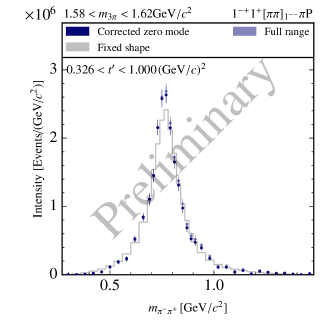
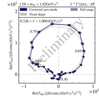
Figure 1: Results for the dynamic isobar amplitude of the spin-exotic wave for a single bin in $m_{3\pi}$ and $t^{\prime}$ in two different representations. The resulting intensity distribution is shown on the left, and the Argand diagram on the right. The gray line indicates the constraint used to resolve the zero-mode ambiguity.

The result for a single $(m_{3\pi},t^{\prime})$ bin is shown in Fig.1, we see, that the resulting dynamic isobar amplitude is dominated by the $\rho(770)$ resonance, as expected. The fixed Breit-Wigner amplitude is a good approximation to the dynamic isobar amplitude, with some significant deviations, especially in the peak region. Such deviations might be caused by non-resonant contributions to the process or re-scattering effects with the third pion.

Looking at the dependence of the freed-isobar results on the $m_{3\pi}$ bin, as shown in Fig. 2, we find a nice correlation of the intensity distributions in $m_{3\pi}$ and $m_{\xi^{\,0}}$, which corresponds to the dominating decay $\pi_{1}^{-}(1600)\to\rho(770)\pi^{-}$. The coherent sum of all $m_{\xi^{\,0}}$ has a similar peak position and width, as the result of the conventional analysis in Ref. massIndepPaper , but a higher total intensity. This shows that the $\pi_{1}^{-}(1600)$ resonance found in the conventional analysis of Ref. massDepPaper is not an artifact of the fixed dynamic isobar amplitudes used.

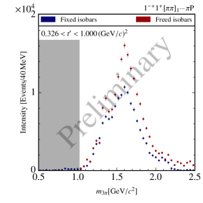
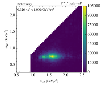
Figure 2: Results of the freed-isobar analysis of the spin-exotic wave as a function of $m_{3\pi}$. The two-dimensional intensity distribution is shown on the right and the coherent sum of all $m_{\xi^{\,0}}$ bins on the left, compared to the results of the conventional PWA.

5 Conclusions

We performed an extended freed-isobar PWA for diffractive $3\pi$ production, for which the Compass spectrometer has collected large exclusive data set of $46\times 10^{6}$ events. In this analysis, we encountered continuous mathematical ambiguities—zero modes—, which are identified and resolved. The results for the spin-exotic wave showed, that the dynamic isobar amplitude is dominated by the $\rho(770)$ resonance, as expected. However, some small but significant deviations from a pure Breit-Wigner shape are visible. We compare our findings to the conventional PWA method and find a peak compatible with the $\pi_{1}^{-}(1600)$ resonance of Refs. massIndepPaper ; massDepPaper .

References

- (1) Compass collaboration (C. Adolph et al.), Phys.Rev. D95 (2017) no.3, 032004
- (2) Compass collaboration (R. Akhunzyanov et al.), arXiv:1802.05913 [hep-ex] (2018)
-
(3)
F. Krinner, D. Greenwald, D. Ryabchikov, B. Grube, and S. Paul,
Phys. Rev. D97 (2018), 114008