Self-bound ultra dilute Bose mixtures within Local Density Approximation

Abstract

We have investigated self-bound ultra dilute bosonic binary mixtures at zero temperature within Density Functional Theory using a Local Density Approximation. We provide the explicit expression of the Lee-Huang-Yang correction in the general case of heteronuclear mixtures, and investigate the general thermodynamic conditions which lead to the formation of self-bound systems. We have determined the conditions for stability against the evaporation of one component, as well as the mechanical and diffusive spinodal lines. We have also calculated the surface tension of the self-bound state as a function of the inter-species interaction strength. We find that relatively modest variations of the latter result in order-of-magnitude changes in the calculated surface tension. We suggest experimental realizations which might display the metastability and phase separation of the mixture when entering regions of the phase diagram characterized by negative pressures. Finally, we show that these droplets may sustain stable vortex and vortex pairs.

I Introduction

The existence of self-bound ultra dilute quantum droplets, made of atoms of a binary mixture of Bose-Einstein condensates, was predicted by Petrov Pet15 and has been experimentally confirmed very recently Cab18 ; Sem18 . The stability of these droplets can be explained as deriving from a subtle balance between the intra-species repulsive atom-atom interaction, and a tunable inter-species attractive interaction.

When the attraction between the two atomic species becomes larger than the single-species average repulsion, the mixture is expected to collapse according to mean-field (MF) theory. Possible stabilization mechanisms preventing the collapse of the mixture triggered by an attractive interaction have been proposed, as e.g. three-body correlations Bul02 , spin-orbit coupling Zha15 and quantum fluctuations (Lee-Huang-Yang (LHY) mechanism Lee57 ). In the latter case, the effective repulsion provided by the first beyond-mean-field (BMF) correction to the energy is enough to prevent the collapse and to stabilize the system, i.e. a density exists where these contributions balance each other and the droplets become self-bound, stable systems. The stabilization mechanism resulting from the inclusion of the LHY correction is also responsible for the existence of self-bound aggregates in one component dipolar systems Kad16 ; Fer16 ; Cho16 ; Bai16 (where the anisotropic character of the dipole-dipole forces leads to the formation of filament-like self-bound droplets with highly anisotropic properties), in Rabi-coupled Bose-Bose mixtures Cap17 and in low-dimensional mixtures Pet16 .

The formation of liquid drops in a Bose-Bose mixture has been recently addressed using the diffusion Monte Carlo (DMC) method Cik18 , confirming the prediction for the stability of self-bound bosonic mixtures Pet15 . More recently, the properties of uniform Bose mixtures have been analyzed using the variational hypernetted-chain Euler Lagrange (HNC-EL) method Sta18 , which includes pair correlations non-perturbatively and turns out to be computationally very fast as compared to the DMC method. In particular, the conditions for having a self-bound, stable mixture of ³⁹K atoms in two different internal states have been studied within the HNC-EL approach. Deviations from a universal dependence on the $s$-wave scattering lengths are found in spite of the low density of the systems Sta18 .

These ultra dilute and weakly interacting quantum liquids –whose densities are orders of magnitude lower than that of the prototypical quantum fluid, namely liquid helium– can be ideal platforms to benchmark quantum many-body theories in actual experiments, and to study processes more difficult to address in the case of liquid helium. For this reason, determining the properties of the underlying uniform system is of special interest in itself and also represents a first step towards a better understanding of self-bound droplets.

In this work we study, within a density functional theory (DFT) approach in a Local Density Approximation (LDA), Bose-Bose mixtures at zero temperature ($T$); in particular, we address the thermodynamic conditions which lead to the formation of self-bound states of the system. We study the general case of heteronuclear mixtures, which has not been considered before within the beyond-mean-field approach to Bose mixtures. As a case of study we discuss in detail a ²³Na-⁸⁷Rb mixture. In order to make a comparison with previous theoretical works, we also address a Bose-Bose mixture with equal masses, made of two hyperfine states of ³⁹K.

This work is organized as follows. In Sec. II we present the DFT approach to Bose-Bose mixtures. The method is applied in Sec. III, within LDA, to the description of the uniform system, allowing us to determine the main characteristics of the stability phase diagram, in particular the mechanical and diffusive spinodal lines obtained as outlined in the Appendix. The surface tension of the mixture is calculated in Sec. IV as a function of the inter-species attraction, and the structure of selected mixed droplets is presented in Sec. V. We show that these droplets may sustain stable vortex and vortex pairs in Sec. VI. Finally, a summary and outlook are given in Sec. VII.

II Density Functional approach

Figure 1: Solid line is the $P=0$ curve in the $(n_{1},n_{2})$ plane for the ²³Na-⁸⁷Rb mixture with $a_{12}=-80\,a_{0}$. The big dot is the point of minimum energy per particle of the $P=0$ curve. The dotted lines correspond to the configurations in the $(n_{1},n_{2})$ plane with chemical potential of one species equal to zero, $\mu_{1}=0$ and $\mu_{2}=0$, respectively. In the closed narrow region delimited by these lines the system has both chemical potentials negative.

Let us consider a uniform Bose-Bose mixture with two components (with masses $m_{1}$ and $m_{2}$) in a volume $V$, interacting with coupling constants $g_{11}=4\pi a_{11}\hbar^{2}/m_{1}$, $g_{22}=4\pi a_{22}\hbar^{2}/m_{2}$, and $g_{12}=2\pi a_{12}\hbar^{2}/m_{r}$, where $m_{r}=m_{1}m_{2}/(m_{1}+m_{2})$ is the reduced mass. The intra-species $s$-wave scattering lengths $a_{11}$ and $a_{22}$ are both positive, while the inter-species $a_{12}$ is negative. The total number of bosons is $N=N_{1}+N_{2}$.

In the following $n_{1}$, $n_{2}$ are the number densities, normalized such that $\int_{V}n_{1}\,{\rm d}{\bf r}=N_{1}$ and $\int_{V}n_{2}\,{\rm d}{\bf r}=N_{2}$. Equivalently, we will also characterize the homogeneous mixture with the total number density, $n=n_{1}+n_{2}$, and concentration of the species 2, $Y=n_{2}/n$.

Although a precise knowledge of the finite-range details of the interatomic potential might be necessary for a more accurate description of such system Sta18 , we consider the simpler description where the $s$-wave scattering lengths are assumed to be enough to fully characterize the inter-particle interactions, and leave to subsequent studies attempts to go beyond the contact interaction approximation. This strategy is similar to that successfully followed within the DFT approach to liquid helium and droplets Dal95 ; Bar06 ; Anc17 .

Within the DFT framework, the total energy of the system is given by

$$E = \int d{\bf r}\left\{\sum_{i}\left[{\hbar^{2}\over 2m_{i}}|\nabla\Psi_{i}|^{2}+{1\over 2}g_{ii}n_{i}^{2}\right]+g_{12}|\Psi_{1}|^{2}|\Psi_{2}|^{2}\right\}$$ (1)

$$+ E_{\rm LHY}\,,$$

where $n_{i}=|\Psi_{i}|^{2}$ and $i=1,2$. $E_{\rm LHY}$ is the BMF Lee-Huang-Yang term, which is necessary in order to yield self-bound configurations Pet15 .

Functional minimization of the above functional leads to the Euler-Lagrange (EL) equations

$$\left[-{\hbar^{2}\over 2m_{i}}\nabla^{2}+V_{i}(n_{1},n_{2})\right]\Psi_{i}=\mu_{i}\Psi_{i}\,,$$ (2)

where $\mu_{i}$ is the chemical potential of the $i$-species and

$$V_{i}=g_{ii}n_{i}+g_{12}n_{j}+{\delta E_{\rm LHY}\over\delta n_{i}}\quad\,(j\neq i)\,.$$ (3)

Eq.(2) is the two-components version of the well-known Gross-Pitaevskii equation gp with the addition of the BMF correction.

The LHY correction to the mean-field theory of the mixture can be expressed as Pet15

$${E_{\rm LHY}\over V}={8\over 15\pi^{2}}\left(\frac{m_{1}}{\hbar^{2}}\right)^{3/2}(g_{11}n_{1})^{5/2}f\left({m_{2}\over m_{1}},{g_{12}^{2}\over g_{11}g_{22}},{g_{22}n_{2}\over g_{11}n_{1}}\right)$$ (4)

where $f>0$ is a dimensionless function defined below.

At the mean-field level, the condensed Bose-Bose mixture collapses when the inter-species attraction becomes stronger than the geometrical average of the intra-species repulsions, $|g_{12}|>\sqrt{g_{11}\,g_{22}}$. Quantum fluctuations, embodied within the LHY energy term, stabilize the mixture. As shown in Ref. Pet15 , the instability manifests itself in the fact that some of the energy contributions in $E_{\rm LHY}$ acquire an imaginary component at small momenta. However, in the region mostly contributing to the LHY term, these modes are found to be insensitive to small variations of $\delta g\equiv g_{12}+\sqrt{g_{11}g_{22}}$, and also to its sign Pet15 . When evaluated at $\delta g=0$, $E_{\rm LHY}$ in Eq. (4) is well defined and free from imaginary contributions. We will use here the same approximation as in Ref. Pet15 to evaluate $E_{\rm LHY}$, namely we set $g_{12}+\sqrt{g_{11}g_{22}}=0$.

The explicit expression for $f$ in Eq.(4) was given in Ref. Pet15 only for the particular case of equal masses. In the more general case $m_{1}\neq m_{2}$, which is addressed here –and considering $\delta g=0$, as discussed above– one finds:

$$f(z,1,x)=\frac{15}{32}\int_{0}^{\infty}k^{2}{\cal F}(k,z,x)\,dk\,,$$ (5)

where

$${\cal F}(k,z,x) = \left\{\frac{1}{2}\left[k^{2}\left(1+\frac{x}{z}\right)+\frac{1}{4}k^{4}\left(1+\frac{1}{z^{2}}\right)\right]+\left[\frac{1}{4}\left[\left(k^{2}+\frac{1}{4}k^{4}\right)-\left(\frac{x}{z}k^{2}+\frac{1}{4z^{2}}\,k^{4}\right)\right]^{2}+{x\over z}\,k^{4}\right]^{1/2}\right\}^{1/2}$$

$$+ \left\{\frac{1}{2}\left[k^{2}\left(1+\frac{x}{z}\right)+\frac{1}{4}k^{4}\left(1+\frac{1}{z^{2}}\right)\right]-\left[\frac{1}{4}\left[\left(k^{2}+\frac{1}{4}k^{4}\right)-\left(\frac{x}{z}k^{2}+\frac{1}{4z^{2}}\,k^{4}\right)\right]^{2}+{x\over z}\,k^{4}\right]^{1/2}\right\}^{1/2}$$

$$- \frac{1+z}{2z}\,k^{2}-(1+x)+\frac{1}{1+z}\,\frac{1}{k^{2}}\left[(1+xz)^{2}+z(1+x)^{2}\right]\,.$$

Here $z\equiv m_{2}/m_{1}$, $x\equiv(g_{22}n_{2})/(g_{11}n_{1})$, and $k$ is dimensionless.

The integral (5) converges in spite of the presence of individually diverging terms in the integrand due to mutual cancellation of the singular terms. For the numerical evaluation of Eq. (4) we found convenient to calculate the improper integral (5) using the following transformation

$$\int_{0}^{\infty}g(k)dk=\int_{0}^{\pi/2}g[\tan(t)]\,\frac{dt}{\cos^{2}(t)}\,.$$

The right-hand side integral has been computed numerically using a Second Euler-McLaurin summation formula refined until some specified degree of accuracy is achieved Pre99 .

In the particular case $N_{1}=N_{2}\equiv N/2$, $m_{1}=m_{2}\equiv m$, and $g_{11}=g_{22}=g_{12}\equiv g=4\pi a\hbar^{2}/m$, Eq. (4) yields the well-known LHY correction for a system of $N$ identical bosons in a volume $V$ (i.e. with density $n$):

$${E_{\rm LHY}\over V}={256\sqrt{\pi}\over 15}\frac{\hbar^{2}}{m}(na)^{5/2}\,,$$ (7)

where we have used

$$f(1,1,1)=\frac{15}{32}\int_{0}^{\infty}k^{2}{\cal F}(k,1,1)\,dk=$$

$$\frac{15}{32}\int_{0}^{\infty}k^{2}\left[\frac{k}{2}\sqrt{8+k^{2}}-\frac{k^{2}}{2}-2+\frac{4}{k^{2}}\right]dk=4\sqrt{2}$$

Within the Local Density Approximation of DFT one can write

$$E_{\rm LHY}=\int_{V}{\cal E}_{\rm LHY}[n_{1}({\bf r}),n_{2}({\bf r})]\,{\rm d}{\bf r}\,,$$ (8)

where the energy density ${\cal E}_{\rm LHY}$ is evaluated at the local densities $n_{1}({\bf r}),n_{2}({\bf r})$:

$${\cal E}_{\rm LHY}\!={8\over 15\pi^{2}}\left(\frac{m_{1}}{\hbar^{2}}\right)^{3/2}[g_{11}n_{1}({\bf r})]^{5/2}f\left(\frac{m_{2}}{m_{1}},1,\frac{g_{22}\,n_{2}({\bf r})}{g_{11}\,n_{1}({\bf r})}\right).$$ (9)

The terms appearing in Eq. (3) are

$${\delta E_{\rm LHY}\over\delta n_{1}}=\frac{\partial{\cal E}_{\rm LHY}}{\partial n_{1}}=$$ (10)

$${8\over 15\pi^{2}}\left(\frac{m_{1}}{\hbar^{2}}\right)^{3/2}g_{11}^{5/2}\,n_{1}^{1/2}\left[{5\over 2}n_{1}f-{g_{22}\,n_{2}\over g_{11}}{\partial f\over\partial x}\right]$$

$${\delta E_{\rm LHY}\over\delta n_{2}}=\frac{\partial{\cal E}_{\rm LHY}}{\partial n_{2}}={8\over 15\pi^{2}}\left(\frac{m_{1}}{\hbar^{2}}\right)^{3/2}g_{11}^{3/2}g_{22}\,n_{1}^{3/2}\,{\partial f\over\partial x}$$ (11)

Figure 2: Densities $n_{1}$ (²³Na, solid line) and $n_{2}$ (⁸⁷Rb, dotted line) as a function of the inter-species $s$-wave scattering length for the minimum energy per particle stable mixtures.

III Uniform system

III.1 Self-bound mixtures

As a case of study we consider in the following a uniform mixture of ²³Na ($a_{11}=54.5\,a_{0}$) and ⁸⁷Rb ($a_{22}=100.4\,a_{0}$) atoms Kno11 ; Mar02 , where $a_{0}$ is the Bohr radius. We will take the inter-atomic scattering length $a_{12}$ as tunable at will. This mixture has been recently studied Wan16 and proven to be a good candidate to investigate interaction-driven effects in a superfluid Bose mixture with a largely tunable inter-species interactions (both repulsive and attractive). We are interested in the regime where self-bound states appear, i.e. when $g_{11},g_{22}>0$, $g_{12}<0$ and $|g_{12}|>\sqrt{g_{11}\,g_{22}}\,$.

The energy per unit volume of the uniform system is

$${\cal E}(n_{1},n_{2})={1\over 2}g_{11}\,n_{1}^{2}+{1\over 2}g_{22}\,n_{2}^{2}+g_{12}n_{1}n_{2}+{\cal E}_{\rm LHY}\,,$$ (12)

and the total energy is $E={\cal E}V$.

At $T=0$, especially relevant stable states of the homogeneous mixture are those that correspond to zero pressure

$$P(n_{1},n_{2})=-{dE\over dV}=n^{2}\frac{\partial}{\partial n}\left(\frac{\cal E}{n}\right)=0\,,$$ (13)

since isolate self-bound droplets must be at equilibrium with vacuum. Recalling that $P(n_{1},n_{2})=-{\cal E}+\mu_{1}n_{1}+\mu_{2}n_{2}\,$, and that

$$\mu_{1} = \frac{\partial{\cal E}}{\partial n_{1}}=g_{11}n_{1}+g_{12}n_{2}+\frac{\partial{\cal E}_{\rm LHY}}{\partial n_{1}}$$

$$\mu_{2} = {\partial{\cal E}\over\partial n_{2}}=g_{22}n_{2}+g_{12}n_{1}+{\partial{\cal E}_{\rm LHY}\over\partial n_{2}}\,,$$ (14)

one obtains for the pressure

$$P(n_{1},n_{2}) = {1\over 2}g_{11}n_{1}^{2}+{1\over 2}g_{22}n_{2}^{2}$$

$$+ g_{12}n_{1}n_{2}-{\cal E}_{\rm LHY}+n_{1}{\partial{\cal E}_{\rm LHY}\over\partial n_{1}}+n_{2}{\partial{\cal E}_{\rm LHY}\over\partial n_{2}}\,,$$

where the BMF terms are evaluated according to Eqs. (10) and (11).

Figure 1 shows the $P=0$ curve in the $(n_{1},n_{2})$ plane computed with $a_{12}=-80\,a_{0}$. The big dot represents the stable state configuration that, for this chosen $a_{12}$ value, has the minimum energy per atom $E/N={\cal E}/n$.

The densities associated to that minimum energy state are shown in Fig. 2 as a function of the interatomic scattering length $a_{12}$. They have been computed as described above, i.e. selecting the minimum energy states among those satisfying the condition $P=0$.

From the results of Fig. 2 it follows that self-bound states appear for $a_{12}<a_{c}\sim-62\,a_{0}$. The critical value $a_{c}$ is consistent with that obtained from the condition $g_{12}=-\sqrt{g_{11}\,g_{22}}$ (which is the instability condition at the mean-field level, i.e. with ${\cal E}_{\rm LHY}=0$), that is $a_{12}\sim-60\,a_{0}$.

In order for an atom of the $i$-th species to be bound in the mixture the chemical potential must be negative, $\mu_{i}<0$. If it is not, the energy will be lowered by removing atoms from the system (evaporation). We have thus computed the limiting curves in the $(n_{1},n_{2})$ plane where the conditions $\mu_{1}=0,\,\mu_{2}=0$ are fulfilled, by using Eqs. (14) for the same value of $a_{12}$ considered above. The results are shown in Fig. 1 where the dotted lines represent the configurations with $\mu_{1}=0$ and $\mu_{2}=0$. Only the points within the closed narrow region shown in the figure are stable against evaporation, i.e. only inside this region the system verifies $\mu_{1}<0$ and $\mu_{2}<0$ simultaneously. Similarly, a very narrow stability region against evaporation has been found for the ³⁹K-³⁹K mixture within the HNC-EL approach Sta18 .

III.2 Spinodal lines

Binary mixtures such as those described here are not thermodynamically stable at all densities $n=n_{1}+n_{2}$, temperatures and relative concentrations $Y=n_{2}/n$. At $T=0$, necessary and sufficient conditions for thermodynamic stability are expressed by the following inequalities Lan67 :

$$\kappa=-V\left(\frac{\partial P}{\partial V}\right)_{N}=n\frac{\partial P}{\partial n}>0\,,$$

$$\left(\frac{\partial\mu_{1}}{\partial Y}\right)_{P}<0\,,$$ (16)

where $\kappa$ is the inverse compressibility –incompressibility– of the system. A positive incompressibility guarantees mechanical stability, and the condition on the chemical potential derivative guarantees diffusive stability. If one of these conditions is violated the mixture cannot exist as a single phase and must undergo phase separation. The coexisting phases that appear may have different densities, different concentrations or both.

Figure 3: Diffusive (solid line) and mechanical (dashed line) spinodal curves for the ²³Na-⁸⁷Rb mixture with $a_{12}=-80\,a_{0}$. The big dot represents the stable, minimum energy per particle mixture at $P=0$. The dotted line is the $P=0$ curve in the $(n,Y)$ plane. The two dash-dot curves correspond to $\mu_{1}=0$ and $\mu_{2}=0$ (also shown in Fig. 1 as a function of $n_{1}$ and $n_{2}$).

The lines obtained setting to zero the above inequalities are called mechanical and diffusive spinodal lines, respectively. Systems such as nucleonic matter, ³He-⁴He liquid mixtures, and partially polarized liquid ³He are examples of highly correlated systems for which the spinodal lines were determined in the past by solving similar equations Bar80 ; Gui95 ; Str87 .

In our system, a straightforward calculation outlined in the Appendix yields:

$$\kappa=g_{11}\,n_{1}^{2}+g_{22}\,n_{2}^{2}+2\,g_{12}\,n_{1}n_{2}+\frac{15}{4}\,{\cal E}_{\rm LHY}\,.$$ (17)

From this expression the mechanical spinodal line $\kappa=0$ can be readily calculated. Similarly, the diffusive spinodal line is obtained by solving the equation:

$$\left({\partial\mu_{1}\over\partial Y}\right)_{P}=0\,.$$ (18)

As outlined in the Appendix, this condition on the $(\partial\mu_{1}/\partial Y)_{P}$ partial derivative can be cast in the following more convenient expression

$$\left({\partial\mu_{1}\over\partial n_{2}}\right)\left({\partial P\over\partial n_{1}}\right)=\left({\partial\mu_{1}\over\partial n_{1}}\right)\left({\partial P\over\partial n_{2}}\right)\,.$$ (19)

The mechanical and diffusive spinodal lines in the $(n,Y)$ plane are shown in Fig. 3 for the ²³Na -⁸⁷Rb mixture with $a_{12}=-80\,a_{0}$. It can be seen from this figure that the stability region against evaporation –the narrow region where the chemical potentials are negative– is considerably reduced by thermodynamic stability conditions, and it is represented in the figure by the small, triangular-shaped region delimited by the two dash-dot lines and the solid line. In particular, the point representing the stable minimum energy mixture is rather close to the diffusive spinodal line. This point is at $P=0$; reducing $n$ at constant $Y$ amounts to decreasing $P$. Hence, from that point down to the diffusive spinodal line, the mixture is in a metastable state at negative pressure. Under these conditions, bubbles might appear in the mixture (cavitation phenomenon), eventually leading to a first order phase transition as thoroughly studied, both theoretically and experimentally, in liquid helium Xio91 ; Jez93 ; Bal02 .

The stability of the ³⁹K-³⁹K mixture has been studied using the HNC-EL method Sta18 , and it was found that the condition that limits the thermodynamic stability of such mixture arises from the mechanical and not from the diffusive spinodal, at variance with the Na-Rb mixture just described. Within the present DFT approach, we have also studied the ³⁹K-³⁹K mixture under similar conditions as those described in Ref. Sta18 , where finite range interactions were used rather than contact interactions as done here. In particular, we have taken $\delta a=-0.156$ (in the same units used in Ref. Sta18 ). The results for the equilibrium densities, chemical potentials and energy per particle are in agreement with their HNC-EL results. In fact we find an equilibrium density ratio $n_{2}/n_{1}=1.385$ to be compared with the HNC-EL result, $n_{2}/n_{1}=1.380$. We find that the total energy per atom is $\epsilon=-3.74$ (in the energy units of Ref. Sta18 ), whereas they find (using an effective range $r_{eff}=43.2$) $\epsilon=-3.364$.

Figure 4: Diffusive (solid line) and mechanical (dashed line) spinodal lines for the ³⁹K-³⁹K mixture with the same parameters as in Ref. Sta18 : $a_{11}=35.2\,a_{0}$, $a_{22}=65.5\,a_{0}$, and $a_{12}=-53.5\,a_{0}$. The big dot represents the stable, minimum energy per particle mixture at $P=0$. The dotted line is the $P=0$ curve in the $(n,Y)$ plane. The two dash-dot curves correspond to $\mu_{1}=0$ and $\mu_{2}=0$

Figure 4 shows the phase diagram of the homogeneous ³⁹K-³⁹K mixture. As found above for the Na-Rb mixture, the stability region is considerably reduced by thermodynamic conditions, and it is represented in the figure by the triangular-shaped region delimited by the two dash-dot lines and the dashed line. At variance with the Na-Rb case, the point representing the stable minimum energy per particle mixture is now close to the mechanical instead to the diffusive spinodal line. This is in agreement with the HNC-EL results Sta18 . We conclude that, not surprisingly, the stability phase diagram is very sensitive to the parameters defining the mixture. As in the Na-Rb case, bubbles are expected to appear in the ³⁹K-³⁹K mixture when the density (thus $P$) is decreased from the stable minimum energy per particle point.

The existence of mechanical and diffusive spinodal lines in self-bound Bose-Bose mixtures might cause dynamic instabilities similar to those characterizing the expansion phase of a highly compressed nuclear spot created in the course of an energetic nucleus-nucleus collision, which triggered an enormous activity in the Nuclear Physics field in the 1980’s, see e.g. Refs. Cug84 ; Str84 ; Bon85 ; Ban85 and references therein. In the BEC case, it is plausible that self-bound mixed droplets compressed by an external trap will expand upon release of the trap, bringing a large portion of the expanding droplet into the unstable region of the phase diagram (e.g. Figs. 3 and 4).

Related effects could be observed in experiments leading to cavitation, similarly to what found in liquid helium Xio91 ; Jez93 ; Bal02 . Cavitation bubbles could be created, e.g., by sweeping a large droplet with a laser beam: the pressure difference due to fore-to-aft asymmetry in the fluid structure around the laser spot could trigger the appearance of cavitation bubbles in the wake of the moving laser. A similar geometry was recently investigated Anc17b in numerical simulations of a moving thin wire in superfluid ⁴He, where vortex dipoles shedding occurred, and where cavitation bubbles formed in the wake of the moving wire, which were found to be responsible for large part of the dissipation accompanying the wire motion.

IV Surface tension of self-bound Bose-Bose mixtures

The appearance of self-bound droplets implies the existence of a surface energy, and a surface tension associated to it. Cikojevič et al. Cik18 have fitted their DMC energies for self-bound droplets of ³⁹K atoms in two different internal states to a liquid droplet expression Bar06 in order to determine the surface tension of the mixture

$$E=E_{v}N+E_{s}N^{2/3}+E_{c}N^{1/3}$$ (20)

where $E_{v}$, $E_{s}$ and $E_{c}$ are volume, surface and curvature energies. The surface tension of the fluid is estimated as $\sigma=E_{s}/(4\pi r_{0}^{2})$, where the bulk radius $r_{0}$ is related to the equilibrium density of the liquid $n_{0}$ as $4\pi r_{0}^{3}n_{0}/3=1$, implicitly assuming that the radii of the density profiles for both species are sensibly the same.

Within DFT, one may address the surface tension of the mixture avoiding the fit procedure to a series of calculated droplets. The surface tension $\sigma$ –actually the grand potential per unit surface Lan67 – of a fluid planar free surface is determined along the saturation line of the liquid-vapor (or liquid-liquid) two-phase equilibrium. In the present case, the line reduces to the $P=0$ point, as the mixture is at $T=0$. If the $z$-axis is taken perpendicular to the free surface, one has

$$\sigma{\cal A} = E-\mu_{1}N_{1}-\mu_{2}N_{2}=$$

$$\int{\rm d}{\mathbf{r}}\left\{{\cal E}[n_{1}({\mathbf{r}}),n_{2}({\mathbf{r}})]-\mu_{1}n_{1}({\mathbf{r}})-\mu_{2}n_{2}({\mathbf{r}})\right\}=$$

$${\cal A}\int_{-\infty}^{\infty}dz\left\{{\cal E}[n_{1}(z),n_{2}(z)]-\mu_{1}n_{1}(z)-\mu_{2}n_{2}(z)\right\}\,,$$

where ${\cal A}$ is the free surface area.

To avoid the complication of imposing different boundary conditions for the density profiles at the opposite ends of the simulation cell, it is more convenient to use a “slab” geometry characterized by a uniform density in the ($x$,$y$) plane and two “liquid”-vacuum planar interfaces perpendicular to the $z$-axis. Here “liquid” means a self-bound mixture of species $1$ and $2$, whose densities $n_{1},n_{2}$ in the bulk region of the slab are determined by the equilibrium conditions discussed before for the uniform system case.

The energy density of the inhomogeneous system with densities $n_{1}({\mathbf{r}}),n_{2}({\mathbf{r}})$ is, from Eq. (1):

$${\cal E}(n_{1},n_{2})=\frac{\hbar^{2}}{2m_{1}}|\nabla\sqrt{n_{1}}|^{2}+\frac{\hbar^{2}}{2m_{2}}|\nabla\sqrt{n_{2}}|^{2}$$

$$+ \frac{1}{2}g_{11}n_{1}^{2}+{1\over 2}g_{22}n_{2}^{2}+g_{12}n_{1}n_{2}+{\cal E}_{\rm LHY}(n_{1},n_{2})\,.$$

As a case of study, we consider again a mixture of ²³Na and ⁸⁷Rb atoms. We will look for self-bound states (i.e. $a_{12}<-62\,a_{0}$, as determined from the uniform system calculation in the previous Sec.) of a number of atoms $N_{1},N_{2}$ contained in a cell of sides $(L_{x},L_{y},2L)$. The size $2L$ of the cell along $z$ is chosen in such a way to guarantee a wide enough region outside the slab, where the densities $n_{1},n_{2}$ are essentially zero.

We have obtained the equilibrium densities $n_{1}({\bf r})=|\Psi_{1}({\bf r})|^{2}$ and $n_{2}({\bf r})=|\Psi_{2}({\bf r})|^{2}$ from the solution of the coupled EL Eqs. (2) in the slab geometry for different values of the interaction strength $a_{12}$. Several total density profiles, $n(z)=n_{1}(z)+n_{2}(z)$, for the calculated equilibrium configurations are shown in Fig. 5. Only one-half of the simulation cell containing the slab is shown for clarity. Note the very different shapes of the interface separating a bulk region in the left part of the figure and the vacuum region to the right, and that the more negative is $a_{12}$, the narrower the interface.

Figure 5: Total density profiles $n(z)=n_{1}(z)+n_{2}(z)$ for the ²³Na-⁸⁷Rb mixture, computed for different values of $a_{12}$.

We have calculated the surface tension using these $n_{1}(z),n_{2}(z)$ profiles

$$\sigma=\int_{0}^{L}dz\big{[}{\cal E}(n_{1}(z),n_{2}(z))-\mu_{1}n_{1}(z)-\mu_{2}n_{2}(z)\big{]}\,.$$ (23)

The results are shown in Fig. 6 on a logarithmic scale, to underline the huge variation of $\sigma$ –which spans almost four orders of magnitude– as the inter-species interaction strength is varied.

Figure 6: Calculated surface tension of the self-bound systems for the ²³Na-⁸⁷Rb mixture as a function of $a_{12}$ (squares). The solid line is drawn to guide the eye.

V Droplets.

We describe here numerical calculations of isolate, spherical self-bound droplets made of $N_{1}$ atoms of ²³Na and $N_{2}$ atoms of ⁸⁷Rb. To this end, we have solved the coupled EL Eqs. (2) to obtain the densities, $n_{1}(r)$ and $n_{2}(r)$, for different values of the inter-particle interaction strength $a_{12}$.

In our calculations we arbitrarily fix the radius $R$ of the droplet to be computed. The values of $N_{1}$ and $N_{2}$ thus depend upon the chosen value of $a_{12}$, and must be such that in the central part of the droplet, where the density profiles are sensibly constant, the associated densities $n_{1},n_{2}$ are those of the lowest energy per particle state of the mixture in the uniform system (see Fig. 2). In practice, we started our calculation with a density profile which reproduces, at the center of the droplet, the bulk equilibrium values $(n_{1}^{b},n_{2}^{b})$ predicted for the uniform system. Then $N_{i}$ is fixed so that $N_{i}=4\,\pi R^{3}n_{i}^{b}/3$.

Figure 7: Radial density profiles for the droplet state of the ²³Na-⁸⁷Rb mixture with $a_{12}=-75\,a_{0}$. Solid line corresponds to the total density, dashed and dotted lines to ²³Na ($n_{1}$), and to ⁸⁷Rb ($n_{2}$), respectively.

Figure 8: ²³Na-⁸⁷Rb droplet total energy per atom as a function of $a_{12}$. The solid line is drawn to guide the eye.

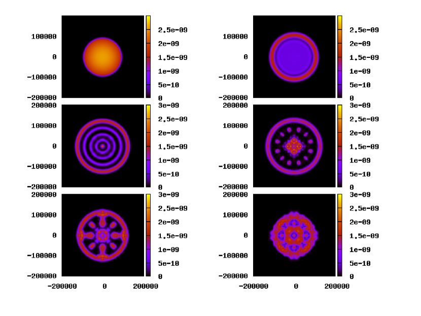
Figure 9: Selected frames (from left to right, from top to bottom) during the real-time evolution of an initially compressed self-bound ²³Na-⁸⁷Rb droplet. Color map represents the total density (in $a_{0}^{-3}$). Lengths are in units of $a_{0}$.

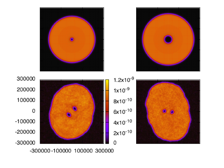
Figure 10: From left to right, from top to bottom: (i) singly-quantized vortex in a ²³Na-⁸⁷Rb droplet; (ii) doubly-quantized vortex; (iii) and (iv) shows the two-vortex structure resulting from the dynamical decay of (ii). (iii) and (iv) are taken at different times during the evolution initiated from (ii), and shows the apparent rotation (counter clockwise) of the droplet/vortices system. Color map represents the total density (in $a_{0}^{-3}$). Lengths are in units of $a_{0}$.

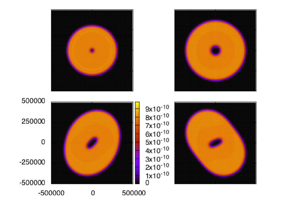
Figure 11: From left to right, from top to bottom: (i) singly-quantized vortex in a ³⁹K-³⁹K droplet; (ii) doubly-quantized vortex; (iii) and (iv) shows the distorted-core structure resulting from the dynamical evolution of (ii). (iii) and (iv) are taken at different times during the evolution initiated from (ii), and shows the apparent rotation (counter clockwise) of the droplet/core system. Color map represents the total density (in $a_{0}^{-3}$). Lengths are in units of $a_{0}$.

If we choose instead values of the densities which are far from the equilibrium ones, during the minimization process the excess atoms move towards the outer droplet surface and form a background of excess species. The experimental counterpart of such behavior is the evaporation which accompanies any excess species in the forming droplet.

We show in Fig. 7 the density profiles for one such self-bound droplet corresponding to $R=10^{5}\,a_{0}$ and $a_{12}=-75\,a_{0}$. The total number of atoms contained in the droplet is $N\sim 3.5\times 10^{6}$. Figure 8 shows the droplet energy per atom $E/(N_{1}+N_{2})$ for different $a_{12}$ values. The crossing with the $E=0$ line marks the critical value of $a_{12}$ for the formation of a self-bound droplet.

As discussed previously, self-bound mixtures, when subject to a tensile stress, might enter the metastable negative pressure region and eventually reach the mechanical or diffusive instability line. A way to achieve this experimentally would be to compress a fairly big self-bound droplet by applying an external harmonic trap and then let it expand upon releasing the trap, thus bringing a large portion of the bulk of the expanding droplet into the negative pressure region of the phase diagram (e.g. Figs. 3 and 4).

We have simulated this process numerically, using the time-dependent version of the EL equations governing the dynamics of the mixed droplets. We consider here a self-bound droplet of radius $R=10^{5}\,a_{0}$, made of $2.7\times 10^{6}$ Na atoms and $3.6\times 10^{6}$ Rb atoms, interacting with $a_{12}=-80\,a_{0}$ and subject to the compression exerted by an external isotropic harmonic potential with frequency $\omega=2\pi\times 400$ Hz. As a result we observe, after the trap release, a sudden expansion of the compressed droplet accompanied by the formation of well separated radial shells and the fragmentation of the latters into smaller radially distributed clusters, each characterized by the same relative composition of the original droplet. After such initial expansion, the collection of fragments contracts, eventually leading to a radial oscillation of the whole structure. Several snapshots taken during such evolution are shown in Fig. 9. Note that symmetry breaking of the densities of the emerging fragments occurs in spite of the spherical symmetry of the initial configuration and contact atom-atom interactions, which is a common manifestation of modulation instability against azimuthal perturbations.

The details of the fragmentation process depend on the amount of the initial compression. A gentle squeezing of the droplet leads instead to the excitation of an intrinsic mode of the droplet in the form of a breathing oscillation, whose frequency depends upon the incompressibility of the mixture, Eq. (17).

VI Vortices

Finally, we briefly address vortical states in mixed self-bound droplets. In particular, we study the stationary states where a singly quantized vortex and a doubly-quantized vortex are nucleated in the center of the droplet. Vortical states in self-bound droplets have been studied recently in dipolar Bose droplets Cid18 , and found to be unstable as a consequence of the very anisotropic nature of such droplets. The spherical mixed Bose droplets studied in our work, however, might sustain stable vortices. Swirling self-bound droplets made of Bose mixtures have been studied recently in Ref. Kar18 , where it was found that self-trapped vortex “tori” with double vorticity are stable topological defects when the droplet exceeds a certain critical size.

We consider first a ²³Na-⁸⁷Rb droplet of radius $R=2\times 10^{5}\,a_{0}$ for $a_{12}=-75\,a_{0}$, and imprint on each component a vortex with quantization number $m$ by multiplying the pure droplet wave function by a phase factor $e^{im\phi}$, $\phi$ being the azimuthal angle, and evolve this initial configuration in imaginary time until a stable structure is found. A singly (doubly) quantized vortex is shown in the top left(right) panel of Fig. 10.

We have studied the dynamical stability of these two configurations by evolving them in real time after a quadrupolar perturbation has been added to the droplet by multiplying its wave function by the phase $e^{i\epsilon xy}$ (note that this adds kinetic energy but not angular momentum to the system). We have chosen the small constant $\epsilon$ such that the applied perturbation increases the kinetic energy of the system by a few percent.

While the singly-quantized vortex is robust against quadrupolar perturbation, we have found that the doubly-quantized vortex rapidly decays into a pair of singly-quantized vortices. Such vortices are shown in the bottom panels of Fig. 10. As a result of the angular momentum associated with the two vortices, the vortex dimer rotates as a rigid body around the center of mass of the droplet.

The velocity field associated with the added quadrupolar phase, together with the angular momentum stored in the doubly-quantized vortex result in surface capillary waves, which distort the droplet surface and are responsible for the apparent rotation of the droplet as a whole Cop17 , as shown in the bottom panels of Fig. 10. In this particular case, the vortex dimer appears to rotate with a frequency $\omega=3\times 10^{15}$ a.u. It is worth mentioning that, at variance with vortices and vortex arrays in expanding unbound condensates, these vortical configurations are stable and similar to those recently found in rotating ⁴He droplets Gom14 ; Anc18 . A more systematic study of vortex arrays in self-bound droplets and the merging of droplets hosting vortices is currently underway Pi18 .

A qualitative similar behavior is observed for the ³⁹K-³⁹K mixed droplet under similar conditions. Fig. 11 shows the fate of a doubly-quantized vortex in a K-K droplet subject to the same perturbation described previously. The vortex decays in a close pair of singly-quantized vortices, as shown in the lower panels of Fig. 11 resembling a partially fused vortex dimer. Yet, these results seem to indicate that, under suitable conditions, the $m=2$ vortex may represent a robust, stable topological defect in mixed Bose droplets, as indeed found in Ref.[Kar18, ].

VII Summary and outlook

We have investigated the zero temperature phase diagram of self-bound ultra dilute bosonic mixtures made of two different species within the DFT-LDA approach, providing an explicit expression for the Lee-Huang-Yang correction in this general case. We determined the general thermodynamic conditions which permit the formation of self-bound systems. To this end, we have obtained simple expressions to calculate the mechanical and diffusive spinodal lines. We have shown that, depending on the mixture, the thermodynamic condition that limits its stability may be either of the spinodal lines, and found, in agreement with previous work on equal species mixtures, that the region of stability in the $(n_{1},n_{2})$ plane of compositions is extremely narrow.

The appearance of self-bound droplets implies the existence of a surface tension, at variance with most of cold gases, which are metastable, unbound systems. We have thus calculated the surface tension of the mixture free-surface and the density profile of some selected droplets. In particular, our results show that the surface tension changes by orders of magnitude when the inter-species interaction changes by only a factor of two.

The realization of stable, self-bound ultra dilute mixtures opens the possibility of studying phenomena that are otherwise restricted to high-densities, strongly correlated superfluids like liquid helium and liquid helium mixtures, such as e.g. cavitation Xio91 ; Jez93 ; Bal02 , free-droplet merging Pi18 , 1D or 3D droplet collisions and merging Ast18 ; Gal18 or rotating free-droplets Gom14 ; Anc18 ; Kar18 . In a similar context, the possibility of creating self-bound Bose-Fermi droplets Rak18 opens the possibility to extend to these ultra dilute systems the study of, e.g., cavitation Gui95 and swirling properties of the prototypical Bose-Fermi quantum mixture, namely the ³He-⁴He fluid mixture Bar06 .

*

Appendix A

We detail in this Appendix the derivation of the mechanical and diffusive spinodal lines. We first calculate the incompressibility of the mixture:

$$\kappa=-V\left(\frac{\partial P}{\partial V}\right)_{N}=n\,\frac{\partial P}{\partial n}\,.$$ (1)

From Eq. (15),

$${dP\over dV} =-{d{\cal E}\over dV}+n_{1}{d\mu_{1}\over dV}+\mu_{1}{dn_{1}\over dV}+n_{2}{d\mu_{2}\over dV}+\mu_{2}{dn_{2}\over dV}$$ (2)

$$=n_{1}{d\mu_{1}\over dV}+n_{2}{d\mu_{2}\over dV}\,.$$

Using Eq. (13) one finds:

$$V{dP\over dV} =-\left[n_{1}^{2}\left(g_{11}+{\partial^{2}{\cal E}_{\rm LHY}\over\partial n_{1}^{2}}\right)+n_{2}^{2}\left(g_{22}+{\partial^{2}{\cal E}_{\rm LHY}\over\partial n_{2}^{2}}\right)\right.$$ (3)

$$\left.+2n_{1}n_{2}\left(g_{12}+{\partial^{2}{\cal E}_{\rm LHY}\over\partial n_{1}\partial n_{2}}\right)\right]\,.$$

Now:

$${\partial^{2}{\cal E}_{\rm LHY}\over\partial n_{1}^{2}} ={8\over 15\pi^{2}}\left(\frac{m_{1}}{\hbar^{2}}\right)^{3/2}g_{11}^{5/2}\left[{15\over 4}n_{1}^{1/2}f-3{g_{22}n_{2}\over g_{11}n_{1}^{1/2}}{\partial f\over\partial x}\right.$$ (4)

$$\left.+{g_{22}^{2}n_{1}^{2}\over g_{11}^{2}n_{1}^{3/2}}{\partial^{2}f\over\partial x^{2}}\right]\,,$$

$${\partial^{2}{\cal E}_{\rm LHY}\over\partial n_{2}^{2}} ={8\over 15\pi^{2}}\left(\frac{m_{1}}{\hbar^{2}}\right)^{3/2}g_{11}^{1/2}g_{22}^{2}n_{1}^{1/2}{\partial^{2}f\over\partial x^{2}}\,,$$ (5)

$${\partial^{2}{\cal E}_{\rm LHY}\over\partial n_{1}\partial n_{2}} ={8\over 15\pi^{2}}\left(\frac{m_{1}}{\hbar^{2}}\right)^{3/2}g_{11}^{5/2}n_{1}^{1/2}\left[{3\over 2}{g_{22}\over g_{11}}{\partial f\over\partial x}\right.$$ (6)

$$\left.-{g_{22}^{2}n_{2}\over g_{11}^{2}n_{1}}{\partial^{2}f\over\partial x^{2}}\right]\,.$$

Noticing that the terms containing $\partial f/\partial x$ and $\partial^{2}f/\partial x^{2}$ in the second derivatives of ${\cal E}_{\rm LHY}$ cancel out, i.e.

$$n_{1}^{2}{\partial^{2}{\cal E}_{\rm LHY}\over\partial n_{1}^{2}}+n_{2}^{2}{\partial^{2}{\cal E}_{\rm LHY}\over\partial n_{2}^{2}}+2n_{1}n_{2}{\partial^{2}{\cal E}_{\rm LHY}\over\partial n_{1}\partial n_{2}}$$ (7)

$$={2\over\pi^{2}}\left(\frac{m_{1}}{\hbar^{2}}\right)^{3/2}(g_{11}n_{1})^{5/2}\,f={15\over 4}{\cal E}_{\rm LHY}\;,$$

one finally finds for $\kappa$ the expression in Eq. (17).

The diffusive spinodal line

$$\left({\partial\mu_{1}\over\partial Y}\right)_{P}=0$$ (8)

can be easily computed by transforming the above equation using the method of the Jacobians Lan67 . At constant temperature,

$$\left(\frac{\partial\mu_{1}}{\partial Y}\right)_{P}=\frac{\partial(\mu_{1},P)}{\partial(Y,P)}=\frac{\frac{\partial(\mu_{1},P)}{\partial(n_{1},n_{2})}}{\frac{\partial(Y,P)}{\partial(n_{1},n_{2})}}$$ (9)

From the definition of the chemical potentials and pressure at zero $T$, it is easy to show that

$$\frac{\partial(\mu_{1},P)}{\partial(Y,P)}=\frac{n^{2}n_{2}\left\{\left[\frac{\partial^{2}{\cal E}}{\partial n_{1}\partial n_{2}}\right]^{2}-\frac{\partial^{2}{\cal E}}{\partial n^{2}_{1}}\frac{\partial^{2}{\cal E}}{\partial n^{2}_{2}}\right\}}{\left\{n_{1}^{2}\frac{\partial^{2}{\cal E}}{\partial n^{2}_{1}}+2n_{1}n_{2}\frac{\partial^{2}{\cal E}}{\partial n_{1}\partial n_{2}}+n_{2}^{2}\frac{\partial^{2}{\cal E}}{\partial n^{2}_{2}}\right\}}\,,$$ (10)

where ${\cal E}$ is the energy density for the uniform system. Thus the diffusive spinodal line can be obtained by solving the equation

$$\left({\partial^{2}{\cal E}\over\partial n_{1}^{2}}\right)\left({\partial^{2}{\cal E}\over\partial n_{2}^{2}}\right)=\left[{\partial^{2}{\cal E}\over\partial n_{1}\partial n_{2}}\right]^{2}$$ (11)

or, equivalently, Eq. (19). Notice that, from the computing viewpoint, both spinodals involve the same ingredients.

References

- (1) D.S. Petrov, Phys. Rev. Lett. 115, 155302 (2015).
- (2) C.R. Cabrera, L. Tanzi, J. Sanz, B. Naylor, P. Thomas, P. Cheiney, and L. Tarruell, Science 359, 301 (2018).
- (3) G. Semeghini, G. Ferioli, L. Masi, C. Mazzinghi, L. Wolswijk, F. Minardi, M. Modugno, G. Modugno, M. Inguscio, and M. Fattori, Phys. Rev. Lett. 120, 235301 (2018).
- (4) A. Bulgac, Phys. Rev. Lett. 89, 050402 (2002).
- (5) Y.-C. Zhang, Z.-W. Zhou, B.A. Malomed, and H. Pu, Phys. Rev. Lett. 115, 253902 (2015).
- (6) T.D. Lee, K. Huang, and C.N. Yang, Phys. Rev. Lett. 106, 1135 (1957).
- (7) H. Kadau, M. Schmitt, M. Wenzel, C. Wink, T. Maier, I. Ferrier-Barbut, and T. Pfau, Nature 530, 194 (2016).
- (8) I. Ferrier-Barbut, H. Kadau, M. Schmitt, M. Wenzel, and T. Pfau, Phys. Rev. Lett. 116, 215301 (2016).
- (9) L. Chomaz, S. Baier, D. Petter, M.J. Mark, F. Wachtler, L. Santos, and F. Ferlaino, Phys. Rev. X 6, 041039 (2016).
- (10) D. Baillie, R.M. Wilson, R.N. Bisset, and P.B. Blakie, Phys. Rev. A 94, 021602(R) (2016).
- (11) A. Cappellaro, T. Macri, G.F. Bertacco, and L. Salasnich, Sci. Rep. 7, 13358 (2017).
- (12) D.S. Petrov and G.E. Astrakharchik, Phys. Rev. Lett. 117, 100401 (2016).
- (13) V. Cikojević K. Dželalija, P. Stipanović, L. Vranješ Markić, and J. Boronat, Phys. Rev. B 97, 140502(R) (2018).
- (14) C. Staudinger, F. Mazzanti, and R.E. Zillich, arXiv:1805.06200.
- (15) F. Dalfovo, A. Lastri, L. Pricaupenko, S. Stringari, and J. Treiner, Phys. Rev. B 52, 1193 (1995).
- (16) M. Barranco, R. Guardiola, S. Hernández, R. Mayol, J. Navarro, and M. Pi, J. Low Temp. Phys. 142, 1 (2006).
- (17) F. Ancilotto, M. Barranco, F. Coppens, J. Eloranta, N. Halberstadt, A. Hernando, D. Mateo, and M. Pi, Int. Rev. Phys. Chem. 36, 621 (2017).
- (18) L.P. Pitaevskii, Sov. Phys. JETP 13, 451 (1961); E.P. Gross, Nuovo Cimento 20, 454 (1961); J. Math. Phys. 4, 195 (1963).
- (19) W.H. Press, S.A. Teukolsky, W.T. Vetterling, and B.P. Flannery, Numerical Recipes in Fortran 77: The Art of Scientific Computing, 2nd. ed. (Cambridge University Press, New York, 1999).
- (20) S. Knoop, T. Schuster, R. Scelle, A. Trautmann, J. Appmeier, M.K. Oberthaler, E. Tiesinga, and E. Tiemann, Phys. Rev. A 83, 042704 (2011).
- (21) A. Marte, T. Volz, J. Schuster, S. Durr, G. Rempe, E.G.M. van Kempen, and B.J. Verhaar, Phys. Rev. Lett. 89, 283202 (2002).
- (22) F. Wang, X. Li, D. Xiong, and D. Wang, J. Phys. B: At. Mol. Opt. Phys. 49, 015302 (2016).
- (23) L.D. Landau and E.M. Lifshitz, Physique Statistique (Editions Mir, Moscow 1967).
- (24) M. Barranco and J.R. Buchler, Phys. Rev. C 22, 1729 (1980)
- (25) M. Guilleumas, D.M. Jezek, M. Pi, M. Barranco and J. Navarro, Phys. Rev. B 51, 1140 (1995).
- (26) S. Stringari, M. Barranco, A. Polls, P.J. Nacher, and F. Laloë, J. Physique 48, 1337 (1987).
- (27) Q. Xiong and H.J. Maris, J. Low Temp. Phys. 82, 105 (1991).
- (28) D.M. Jezek, M. Guilleumas, M. Pi, M. Barranco, and J. Navarro, Phys. Rev. B 48, 16582 (1993).
- (29) S. Balibar, J. Low Temp. Phys. 129, 363 (2002).
- (30) J. Cugnon, Phys. Lett. B 135, 374 (1984).
- (31) B. Strack and J. Knoll, Z. Phys. A 315, 249 (1984).
- (32) J.P. Bondorf, R. Donangelo, I.N. Mishustin, C.J. Pethick, H. Schulz, and K. Sneppen, Nucl. Phys. A 443, 321 (1985).
- (33) Sa Ban-Hao and D.H.E. Gross, Nucl. Phys. A 447, 643 (1985).
- (34) F. Ancilotto, M. Barranco, J. Eloranta, and M. Pi, Phys. Rev. B 96, 064503 (2017).
- (35) A. Cidrim, F.E.A. dos Santos, E.A.L. Henn, and T. Macri, Phys. Rev. A 98, 023618 (2018).
- (36) Y.V. Kartashov, B.A. Malomed, L. Tarruell, and L. Torner, Phys. Rev. A 98, 013612 (2018).
- (37) F. Coppens, F. Ancilotto, M. Barranco, N. Halberstadt, and M. Pi, Phys. Chem. Chem. Phys. 19, 24805 (2017).
- (38) L.F. Gomez, K.R. Ferguson, J.P. Cryan, C. Bacellar, R.M.P. Tanyag, C. Jones, S. Schorb, D. Anielski, A. Belkacem, C. Bernando, R. Boll, J. Bozek, S. Carron, G. Chen, T. Delmas, L. Englert, S.W. Epp, B. Erk. L. Foucar, R. Hartmann, A. Hexemer, M. Huth, J. Kwok, S.R. Leone, J.H. S. Ma, F.R. N. C. Maia, E. Malmerberg, S. Marchesini, D.M. Neumark, B. Poon, J. Prell, D. Rolles, B. Rudek, A. Rudenko, M. Seifrid, K.R. Siefermann, F.P. Sturm, M. Swiggers, J. Ullrich, F. Weise, P. Zwart, C. Bostedt, O. Gessner, and A.F. Vilesov, Science 345, 906 (2014).
- (39) F. Ancilotto, M. Barranco and M. Pi, Phys. Rev. B 97, 184515 (2018).
- (40) M.Pi, F. Ancilotto, and M. Barranco, work in progress.
- (41) G.E. Astrakharchik and B.A. Malomed, Phys. Rev. A 98, 013631 (2018).
- (42) A. Gallemí et al., work in progress.
- (43) D. Rakshit, T. Karpiuk, M. Brewczyk, and M. Gajda, arXiv:1801.00346v2.