A nonlocal isoperimetric problem with dipolar repulsion

Abstract

We study a geometric variational problem for sets in the plane in which the perimeter and a regularized dipolar interaction compete under a mass constraint. In contrast to previously studied nonlocal isoperimetric problems, here the nonlocal term asymptotically localizes and contributes to the perimeter term to leading order. We establish existence of generalized minimizers for all values of the dipolar strength, mass and regularization cutoff and give conditions for existence of classical minimizers. For subcritical dipolar strengths we prove that the limiting functional is a renormalized perimeter and that for small cutoff lengths all mass-constrained minimizers are disks. For critical dipolar strength, we identify the next-order $\Gamma$-limit when sending the cutoff length to zero and prove that with a slight modification of the dipolar kernel there exist masses for which classical minimizers are not disks.

1 Introduction

Understanding the emergence of spatial order from basic constitutive interactions is one of the most important problems in the natural sciences. For example, why do the ions of Na⁺ and Cl^- organize themselves into an alternating pattern arranged into a cubic crystal when precipitating from a supersaturated aqueous solution, something that can be readily observed in a simple tabletop experiment? Our present physical understanding is that this process is driven by the competition of repulsive electrostatic interactions between the like ions, attractive interactions between the opposite ions, and a hard-core repulsion at short distances, to minimize the total interaction energy (both quantum mechanical and thermal effects are also present, but are believed to be of secondary importance). In these terms, the fundamental problem was concisely articulated in 1967 by Uhlenbeck [60, p. 581]: “The basic difficulty lies perhaps in the fact that one does not really understand the existence of regular solids from the molecular forces.” For ionic crystals in the much simpler periodic setting, the question goes back much further [10] and was resolved only very recently [7].

The above question becomes even more complicated for problems involving many-body effects. Perhaps the best known example is that of the spatial arrangement of protons and neutrons in nuclear matter, which is relevant both to the shape of ordinary atomic nuclei [29] and the exotic phases of matter in the crust of neutron stars [52]. The same problem is also ubiquitous in various hard and soft condensed matter systems in which mesoscopic phases form as a result of competing attractive and repulsive interactions operating on different scales [55, 6, 47, 49, 30]. The earliest model that captures the competition of short-range attractive forces and long-range repulsive forces in the case of the atomic nuclei was conceived in 1929 by Gamow [24] and further refined by Heisenberg [29] and von Weizsäcker [61]. It is now known as the liquid drop model of the atomic nucleus. In this model, the nucleus is treated as a drop of incompressible liquid held together by surface tension and subject to Coulombic repulsion by the uniformly distributed positive charge of the protons. For dense nuclear matter, the same model is considered within a large periodic box and is known to produce multiple morphologies referred to as nuclear “pasta” phases [52].

Mathematically, the liquid drop model belongs to a class of geometric variational problems in which one minimizes energies of the form (for a non-technical overview, see [12])

$$E(\Omega):=P(\Omega)+\frac{1}{2}\int_{\Omega}\int_{\Omega}G(x-y)\,\,\mathrm{d}x\,\mathrm{d}y,$$ (1.1)

among measurable sets $\Omega\subset\mathbb{R}^{n}$ subject to a mass constraint $|\Omega|=m$ for $m>0$. Here $|\Omega|$ denotes the $n$-dimensional Lebesgue measure of the set $\Omega$, $P(\Omega)$ is the perimeter of $\Omega$, which is a suitable generalization of the surface measure (for precise definitions, see below), and $G(x)$ is some “repulsive” kernel. In the case of the liquid drop model in the whole space, one chooses the Newtonian potential $G(x):=\frac{1}{4\pi|x|}$ and minimizes over all $\Omega\subset\mathbb{R}^{3}$. In a periodic setting, one should instead consider $\Omega$ to be a subset of a large three-dimensional torus, and $G$ should be the periodic Green’s function of the Laplacian (with uniform neutralizing background) [38]. Note that with different spatial dimensionalities and different choices of repulsive kernels the model is also relevant to a number of other physical situations [47, 48, 35, 36]. In fact, the case of dipolar repulsion considered in this paper falls within the above framework as well.

In the mathematical literature, nonlocal isoperimetric problems in which perimeter competes with a nonlocal repulsive term seem to have been largely unnoticed until quite recently, with a notable exception of a paper by Otto on the dynamics of labyrinthine pattern formation in ferrofluids [51], and a paper by Rigot dealing mostly with regularity of minimizers of (1.1) [53]. Gamow’s liquid drop model caught the attention of mathematicians after reappearing as the leading order asymptotic problem in the studies of the Ohta-Kawasaki energy by Choksi and Peletier [13, 14]. Since then the problem has enjoyed a considerable attention. In the following, we review some of the results obtained so far (naturally, the list of references below is not meant to be comprehensive).

The first study of the problem associated with (1.1), in which $\Omega\subset\mathbb{R}^{n}$ and $G(x)=\frac{1}{|x|^{\alpha}}$ is a Riesz kernel with $\alpha\in(0,n)$ was carried out by Knüpfer and Muratov [35, 36]. This setting includes the classical Gamow’s model, for which $n=3$ and $\alpha=1$. For a range of parameters covering the latter, their results establish existence and radial symmetry of minimizers for sufficiently small masses, and non-existence for sufficiently large masses. Radial symmetry for small masses was also independently established by Julin in $\mathbb{R}^{n}$ for all $n\geq 3$ in the case of $G(x)=\frac{1}{|x|^{n-2}}$ [32], and by Bonacini and Cristoferi for a range of Riesz kernels [8]. In bounded domains with a particular choice of boundary conditions, Cicalese and Spadaro proved that minimizers are close to balls in the vanishing mass limit, but cannot be exactly spherical unless the original domain is a ball [15]. A further generalization to all Riesz kernels and nonlocal perimeters is due to Figalli, Fusco, Maggi, Millot and Morini [19] in the spirit of the currently developing theory of nonlocal minimal surfaces (see, for example, [11]). Non-existence of minimizers for large masses for Gamow’s model was also independently established by Lu and Otto [41], and Frank, Killip and Nam provided an explicit estimate for the mass beyond which minimizers do not exist [21]. It is currently an open problem whether the minimizers are balls whenever they exist in the case of Gamow’s model.

On the other hand, minimizers always exist in the periodic setting. Alberti, Choksi and Otto [2] proved uniform distribution of mass, which is a popular first step for approaching the question of periodicity of minimizers. In various low volume fraction regimes, Choksi and Peletier [13] and Knüpfer, Muratov and Novaga [38] proved that the minimizers consist of small isolated droplets, whose shape is asymptotically determined by solutions of the whole space problem for certain masses (as already mentioned, they are presently unknown, although conjectured to be balls; see also [22]). Similar results are also available for Gamow’s model with screening and for the Ohta-Kawasaki energy, which can be understood as a diffuse interface approximation to Gamow’s liquid drop model [14, 48, 26, 27]. In particular, it is proved that in two dimensions the droplets become almost circular. In other regimes, Sternberg and Topaloglu identified stripes as the global minimizers in the case of the two-dimension torus [56], and Morini and Sternberg showed that such patterns also turn out to be minimizers in thin domains [45]. Another class of (anisotropic) nonlocal isoperimetric problems in dimensions $n\geq 2$ in which minimizers are one-dimensional and periodic is given by Goldman and Runa [28], and by Daneri and Runa [18].

In this paper, we study a nonlocal isoperimetric problem described by (1.1) in two space dimensions, $n=2$, in which the kernel $G$ is of dipolar type, i.e., $G(x)\simeq\frac{1}{|x|^{3}}$. This is the interaction experienced at large distances by spins lying on the plane and oriented perpendicularly to it. Just like the classical Gamow’s model, the model under consideration is relevant to the multidomain patterns observed in perpendicularly magnetized thin film ferromagnets [30], as well as ferroelectric films [57], Langmuir monolayers [5] and ferrofluid films subject to a strong perpendicular applied field [54, 31] (for an experimental realization involving a magnetic garnet film, see Figure 1). Note, however, that setting $G(x)=\frac{1}{|x|^{3}}$ would result in an ill-defined problem because of the divergence of the integral defining the nonlocal contribution at short scales. Furthermore, redefining the energy in the spirit of nonlocal minimal surfaces [11] to reduce the integral to that over $\Omega$ and $\Omega^{c}$, up to an additive constant, would not help, either, since the singularity of the kernel is still too strong. Therefore, a genuine regularization at short scale $\delta>0$ is necessary to make sense of the energy in (1.1) with this kind of kernel. This is a novel feature of the considered nonlocal isoperimetric problem compared to those studied previously.

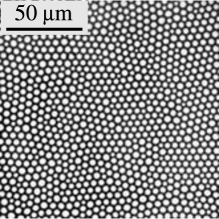
(a)

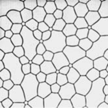
(b)

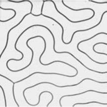
(c)

Figure 1: Domain patterns in a magnetic garnet film with strong perpendicular anisotropy undergoing magnetization reversal driven by the applied magnetic field : a) (approximately) periodic arrangement of bubble domains; b) a network of interconnected stripes; c) a labyrinthine pattern. Reproduced from [30, Figure 5.118].

More specifically, we study the following nonlocal isoperimetric problem, as proposed by Kent-Dobias and Bernoff [34]. We wish to minimize

$$E(\Omega):=\alpha P(\Omega)+\frac{\beta}{2}\int_{\Omega}\int_{\Omega}\frac{g_{\delta}(|x-y|)}{|x-y|^{3}}\,\mathrm{d}x\,\mathrm{d}y,$$ (1.2)

among all finite perimeter sets $\Omega\subset\mathcal{A}_{m}$ of fixed mass $m>0$, i.e., with

$$\mathcal{A}_{m}:=\{\Omega\subset\mathbb{R}^{2}:P(\Omega)<\infty,\ |\Omega|=m\}.$$ (1.3)

Here, $\alpha,\beta>0$ are fixed parameters, $P(\Omega)$ is the perimeter of a measurable set $\Omega$ in the sense of De Giorgi [4]:

$$P(\Omega):=\sup\left\{\int_{\Omega}\nabla\cdot\phi\,\,\mathrm{d}x:\,\phi\in C^{1}_{c}(\mathbb{R}^{2};\mathbb{R}^{2}),\ |\phi|\leq 1\right\},$$ (1.4)

and $g_{\delta}(r):=g(r/\delta)$ is a cutoff function at scale $\delta>0$ that makes the integral well-defined. The specific choice is not essential, so for simplicity we work with $g(r):=\chi_{(1,\infty)}(r)$ throughout the rest of the paper. Note that by a rescaling we can always choose $\alpha=1$.

We are interested in the regime in which $\delta$ is much smaller than the characteristic length scale of minimizers, expressing the physical condition that the regularization happens on the atomic scale, which is much smaller than the scale of the observed patterns. Ultimately, we wish to send the parameter $\delta$ to zero to obtain results that are insensitive to the short-scale cutoff. As we show below, for a meaningful limit as $\delta\to 0$ to exist at fixed value of $m>0$ it is necessary to renormalize the strength $\beta$ of the dipolar interaction. We set $\beta:=\lambda/|\log\delta|$ for some $\lambda>0$ and restrict ourselves to the case $\delta<\frac{1}{2}$. Then the nonlocal term can be rewritten, so that, up to an additive constant depending only on $m$, $\lambda$ and $\delta$, and with $\alpha=1$ the energy in (1.2) is equal to

$$E_{\lambda,\delta}(\Omega):=P(\Omega)-\frac{\lambda}{4|\log\delta|}\int_{\mathbb{R}^{2}}\int_{\mathbb{R}^{2}}|\chi_{\Omega}(x+z)-\chi_{\Omega}(x)|^{2}\,\frac{g_{\delta}(|z|)}{|z|^{3}}\,\mathrm{d}z\,\mathrm{d}x,$$ (1.5)

where $\chi_{\Omega}$ is the characteristic function of the set $\Omega$.

First, we will make sure to demonstrate that minimizers always exist in the generalized sense of consisting of finitely many components that are “infinitely far apart” from each other. In the subcritical regime, $\lambda<1$, we then prove that the $\Gamma$-limit of the energy is given by $(1-\lambda)P(\Omega)$, i.e., the nonlocal term localizes to leading order and renormalizes the perimeter as $\delta\to 0$. Moreover, we prove in Theorem 2.1 that the minimizers of $E_{\lambda,\delta}$ exist also in the classical sense and are in fact disks for all $\delta\ll 1$. The strategy is to make use of sufficiently uniform regularity estimates for minimizers, first on the level of density estimates and then in terms of curvature, as well as stability of the disk with respect to perturbations of curvature.

On the other hand, it is easy to see that disks are no longer classical minimizers for $\delta\ll 1$ as soon as $\lambda>1$, as it is more convenient to split a single disk into multiple components. In fact, by proving that (the components of generalized) minimizers cannot contain disks of radius larger than $r(\delta)>0$ with $r(\delta)\to 0$ as $\delta\to 0$ we see that generalized minimizers cannot be asymptotically well-behaved in this limit. As such, a more precise analysis likely requires further insight into the question whether minimizers are large collections of disks or exhibit stripe-like behavior (see Figure 1).

This naturally brings us to the critical case $\lambda=1$, where in view of the above arguments a transition from classical, radial to non-trivial minimizers occurs for $\delta\ll 1$. In this case, we compute the next-order $\Gamma$-limit as $\delta\to 0$ by observing that the sequence $|\log\delta|E_{1,\delta}(\Omega)$ for a fixed set $\Omega\subset\mathbb{R}^{2}$ of finite perimeter is monotone decreasing in $\delta$. Suitably integrating by parts allows us to represent the limit in a closed form that in fact does not fall within the class of problems given by (1.2). While we cannot directly address the issue of minimizers for the limit, we are able to prove that after modifying the functional by reducing the repulsion at infinity there exist masses for which classical minimizers exist, but are not given by disks. The idea of the proof is to construct a long stripe with large mass whose energy per mass is lower than the energy per mass of disks, ruling out the optimality of any collection of disks.

The paper is organized as follows: In Section 2, we give the precise statements of our main results. In Section 3, we give various representations of the energies and their rescaling behaviors. Section 4 is dedicated to proving existence of generalized minimizers together with control over the number of their components. We also already start to look into the regularity properties of minimizers on a qualitative level. Section 5 contains a thorough discussion of the subcritical case $\lambda<1$, culminating in the proof of Theorem 2.1. The critical case $\lambda=1$, and in particular the existence of non-radial minimizers (Theorem 2.8) for the modified problem is dealt with in Section 6. Finally, Proposition 2.9 characterizing the behavior of generalized minimizers as $\delta\to 0$ in the supercritical case $\lambda>1$ is presented in Section 7.

2 Main results

Our first result identifies the minimizers of $E_{\lambda,\delta}$ over $\mathcal{A}_{m}$ in the subcritical regime of small $\delta$ and $0<\lambda<1$ as disks. The significance of the condition $\lambda<1$ is that even though the nonlocal term renormalizes the perimeter in the limit $\delta\to 0$, we still retain control over the perimeter as is evident by the $L^{1}$-$\Gamma$-limit of $E_{\lambda,\delta}$ for $\delta\to 0$ being given by $(1-\lambda)P(\Omega)$, see Proposition 5.3. This allows us to obtain density estimates for $\Omega$ and the reduced boundary $\partial^{\ast}\Omega$ (for the definition, see, e.g., [42, Chapter 15]) that are uniform in $\delta$. As the localization also turns out to take place in the Euler-Lagrange equation of $E_{\lambda,\delta}$, we can control the curvature of minimizers, which together with a stability property of disks allows us to conclude that the minimizers are disks.

Theorem 2.1.

There exist universal constants $\sigma_{1},\sigma_{2}>0$ with the following properties: Let $0<\lambda<1$ and $0<\delta<\frac{1}{2}$. Under the condition

$$\frac{\lambda}{(1-\lambda)|\log\delta|}\leq\sigma_{1}$$ (2.1)

there exists a minimizer of $E_{\lambda,\delta}$ over $\mathcal{A}_{\pi}$. Furthermore, if

$$\frac{\lambda}{(1-\lambda)^{5}|\log\delta|}\leq\sigma_{2}$$ (2.2)

then the unit disk ${B_{1}\left(0\right)}$ is the unique minimizer of $E_{\lambda,\delta}$ over $\mathcal{A}_{\pi}$, up to translations.

Remark 2.2.

Note that we formulated the theorem for mass $m=\pi$ in order to have a somewhat clean criterion for the smallness of $\delta$ in terms of $\lambda$. However, the rescaling given in Lemma 3.2 allows to obtain a similar result for all masses by replacing $\delta$ with $\sqrt{\frac{\pi}{m}}\delta$ and $\lambda$ with $\frac{\left|\log\left(\sqrt{\frac{\pi}{m}}\delta\right)\right|}{|\log\delta|}\lambda$. Also note that when $m=\pi$ and $\lambda$ approaches 1 for a fixed value of $\delta$, condition (2.1) may still be satisfied, while condition (2.2) fails, indicating the possibility of existence of non-radial minimizers. Whether or not the latter indeed happens for minimizers of $E_{\lambda,\delta}$ over $\mathcal{A}_{\pi}$ is an open problem.

As the first-order $\Gamma$-limit in the critical case $\lambda=1$ degenerates, we have to compute a higher-order $\Gamma$-limit to obtain a helpful limiting description. It turns out that the appropriate sequence to analyze is $|\log\delta|E_{1,\delta}$, as suggested, for example, by the estimate of Proposition 5.1. The $L^{1}$-$\Gamma$-limit is then given by

$$\begin{split}E_{1,0}(\Omega):=-P(\Omega)&+\frac{1}{2}\int_{\partial^{*}\Omega}\int_{\left(\Omega\Delta H_{-}(y)\right)\cap{B_{1}\left(y\right)}}\left|\nu(y)\cdot\frac{x-y}{|x-y|^{3}}\right|\,\mathrm{d}x\,\mathrm{d}\mathcal{H}^{1}(y)\\ &\quad+\frac{1}{2}\int_{\partial^{*}\Omega}\int_{\Omega\setminus{B_{1}\left(y\right)}}\nu(y)\cdot\frac{y-x}{|y-x|^{3}}\,\mathrm{d}x\,\mathrm{d}\mathcal{H}^{1}(y),\end{split}$$ (2.3)

for $\Omega\in\mathcal{A}_{m}$, where $\nu(x)$ is the outer unit normal of $\Omega$ for $x\in\partial^{*}\Omega$ and $H_{-}(y):=\{(x-y)\cdot\nu(y)<0\}$, as determined by the following theorem. A sketch indicating the various domains of integration in (2.3) can be found in Figure 2.

Theorem 2.3.

For every $m>0$, the $\Gamma$-limit of $|\log\delta|E_{1,\delta}$ restricted to $\mathcal{A}_{m}$, with respect to the $L^{1}$-topology as $\delta\to 0$, is given by $E_{1,0}$ in the following sense:

1. (Lower bound) Let $\Omega,\,\Omega_{\delta_{n}}\in\mathcal{A}_{m}$ such that $|\Omega_{\delta_{n}}\Delta\Omega|\to 0$ and $\delta_{n}\to 0$ as $n\to\infty$. Then it holds that

   $$E_{1,0}(\Omega)\leq\liminf_{n\to\infty}|\log\delta_{n}|E_{1,\delta_{n}}(\Omega_{\delta_{n}}).$$ (2.4)

2. (Upper bound) For every set $\Omega\in\mathcal{A}_{m}$, a recovery sequence is given by the constant sequence, i.e., it holds that

   $$E_{1,0}(\Omega)=\lim_{\delta\to 0}|\log\delta|E_{1,\delta}(\Omega)\in\mathbb{R}\cup\{+\infty\}.$$ (2.5)

   In particular, the $\Gamma$-limit coincides with the pointwise limit.

3. (Compactness) For every sequence $\Omega_{\delta_{n}}\in\mathcal{A}_{m}$ such that $\delta_{n}\to 0$ as $n\to\infty$ and

   $$\limsup_{n\to\infty}|\log\delta_{n}|E_{1,\delta_{n}}(\Omega_{\delta_{n}})<\infty,$$ (2.6)

   that in addition satisfies $\Omega_{\delta_{n}}\subset{B_{R}\left(0\right)}$ for some $R>0$, there exists a subsequence (not relabeled) and $\Omega\in\mathcal{A}_{m}$ such that $|\Omega_{\delta_{n}}\Delta\Omega|\to 0$.

Figure 2: Sketch indicating the domains of integration around $y\in\partial^{\ast}\Omega$ in the limiting energy $E_{1,0}(\Omega)$. The first integral term in (2.3) integrates over the dashed region inside the indicated circle, while the second integral term integrates over the dashed region outside that circle. The half-plane $H_{-}(y)$ is shown in gray.

The limiting functional has previously been investigated numerically by Bernoff and Kent-Dobias [34] on the basis of a formal calculation. We are also able to rigorously justify their representation and extend it to sets with a $C^{2}$-boundary.

Proposition 2.4.

If $\Omega\subset\mathbb{R}^{2}$ is a set of finite perimeter with a $C^{2}$-boundary, which is decomposed into positively oriented closed Jordan curves $\gamma_{i}:[0,P_{i}]\to\mathbb{R}^{2}$ of length $P_{i}$ parametrized by arc length for $1\leq i\leq N$, with some $N\in\mathbb{N}$, then it holds that

$$\begin{split}E_{1,0}(\Omega)&=-\sum_{i=1}^{N}P_{i}\left[\log\left(\frac{P_{i}}{2}\right)+2\right]+\frac{1}{2}\sum_{i=1}^{N}\int_{0}^{P_{i}}\int_{-\frac{P_{i}}{2}}^{\frac{P_{i}}{2}}\left(\frac{1}{|s|}-\frac{\dot{\gamma}^{\perp}_{i}(t+s)\cdot\dot{\gamma}^{\perp}_{i}(t)}{|\gamma_{i}(t+s)-\gamma_{i}(t)|}\right)\,\mathrm{d}s\,\mathrm{d}t\\ &\quad-\sum_{i=1}^{N-1}{\sum_{j=i+1}^{N}}\int_{0}^{P_{i}}\int_{0}^{P_{j}}\frac{\dot{\gamma}^{\perp}_{j}(s)\cdot\dot{\gamma}^{\perp}_{i}(t)}{|\gamma_{j}(s)-\gamma_{i}(t)|}\,\mathrm{d}s\,\mathrm{d}t.\end{split}$$ (2.7)

When trying to prove a compactness result for the whole space corresponding to Theorem 2.3, one has to deal with the issue that the functionals $E_{\lambda,\delta}$ have no a priori compactness due to their translational symmetry. Already for fixed parameters this issue manifests itself in minimizing sequences potentially breaking up into multiple pieces which the repulsive nonlocal term then pushes infinitely far apart from each other. In particular, we can in general only hope to prove that minimizers exist in a generalized sense:

Definition 2.5 ([38, Definition 4.3]).

For $m>0$, consider a functional $E:\mathcal{A}_{m}\to\mathbb{R}\cup\{+\infty\}$. We say that a generalized minimizer of $E$ over $\mathcal{A}_{m}$ is a minimizer of the functional

$$\mathcal{S}E\left((\Omega_{i})_{i\in\mathbb{N}}\right)=\sum_{i=1}^{\infty}E(\Omega_{i})$$ (2.8)

defined on the domain

$$\mathcal{SA}_{m}:=\left\{(\Omega_{i})_{i\in\mathbb{N}}:|\Omega_{i}|>0\text{ for at most finitely many }i\in\mathbb{N},P(\Omega_{i})<\infty,\sum_{i=1}^{\infty}|\Omega_{i}|=m\right\}.$$ (2.9)

The main point of this definition is finiteness of the number of pieces, which relies on almost-minimality of minimizing sequences and is not true for arbitrary sequences of sets with uniformly bounded perimeters. The existence of generalized minimizers for all parameters $\lambda,\delta,m>0$ is the main content of Section 4.

Coming back to augmenting Theorem 2.3 with a compactness statement, we see that we have the same issue of sequences of sets breaking up into potentially infinitely many parts in the limit $\delta\to 0$. Instead of dealing with the technicalities of formulating a framework that can handle this issue, we choose to only analyze the compactness properties of minimizers of $E_{1,\delta}$, which in any case is the main consequence one would like to extract from such a statement.

Proposition 2.6.

For $m>0$, generalized minimizers of $E_{1,\delta}$ over $\mathcal{A}_{m}$ are compact in the sense that their number of components is uniformly bounded as $\delta\to 0$, and each component is compact in $L^{1}$ after translation. Additionally, the limiting collection of sets is a generalized minimizer of $E_{1,0}$.

Finally, we turn to investigating the properties of minimizers of $E_{\delta,1}$ for $\delta\ll 1$. We note that we currently do not know what they are for $m>0$ fixed and all $\delta>0$ sufficiently small. In particular, they may or may not be disks, depending on the values of $m$, provided that $\delta\ll 1$. Results of experiments such as the images shown in Figure 1 suggest that in some regimes the minimizers may indeed be disks, while in other regimes the situation may be more complex. Our ansatz-based computations, however, indicate that disks are always preferred over stripe-like constructions that are tractable analytically, both at relatively low mass and in the limit of large masses. One could hope that numerically optimized stripes such as the ones obtained by Bernoff and Kent-Dobias [34] could have lower energy than disks, but this does not seem to be the case. Also a linear stability analysis is unhelpful, as instability of a single disk only occurs at masses at which two disks of equal mass have strictly lower energy. In other words, it seems that splitting a domain into finitely many disks may always decrease energy, thus making stripes always energetically disadvantageous. In fact, one might be tempted to argue that the persistence of balls as generalized minimizers is a universal feature of systems described by (1.1).

In the following we demonstrate that the above view is too simplistic and that the conjecture about the universal optimality of balls in the context of (1.1) is false. Indeed, we will show that under appropriate conditions stripes produce better candidates for generalized minimizers than collections of disks in $\mathbb{R}^{2}$. In order to tilt the favor towards stripes, for $l>0$ we consider the energy

$$F_{\lambda,\delta,l}(\Omega):=P(\Omega)-\frac{\lambda}{4|\log\delta|}\int_{\mathbb{R}^{2}}\int_{\mathbb{R}^{2}}|\chi_{\Omega}(x+z)-\chi_{\Omega}(x)|^{2}K_{\delta,l}(|z|)\,\mathrm{d}z\,\mathrm{d}x,$$ (2.10)

where

$$K_{\delta,l}(r):=\frac{g_{\delta}(r)}{r^{3}}-\frac{r^{2}-2l^{2}}{(r^{2}+l^{2})^{5/2}}.$$ (2.11)

This is precisely the energy of two identical, but oppositely oriented dipolar patches lying in the parallel planes separated by distance $l$. Such a model is, for example, relevant to synthetic antiferromagnets, in which the antiparallel alignment of spins in adjacent layers is favored by antiferromagnetic exchange coupling through a spacer layer (see, e.g., [46]). Heuristically, the kernel behaves as in a dipolar layer on scales $r\lesssim l$, while on large scales the kernel decays faster, thus reducing the long-range repulsion in the far field. Notice that we recover the original energy in the limit $l\to\infty$.

From the point of view of Theorem 2.3, the modification is merely a continuous perturbation:

Lemma 2.7.

For all $l>0$ and $m>0$, the $L^{1}$-$\Gamma$-limit of $F_{1,\delta,l}$ restricted to $\mathcal{A}_{m}$ is given, as $\delta\to 0$, by

$$F_{1,0,l}\left(\Omega\right):=E_{0,1}\left(\Omega\right)+\frac{1}{4}\int_{\mathbb{R}^{2}}\int_{\mathbb{R}^{2}}|\chi_{\Omega}(x+z)-\chi_{\Omega}(x)|^{2}\frac{|z|^{2}-2l^{2}}{(|z|^{2}+l^{2})^{5/2}}\,\mathrm{d}z\,\mathrm{d}x$$ (2.12)

for $\Omega\in\mathcal{A}_{m}$. Also for $F_{1,\delta,l}$ the number of components of generalized minimizers over $\mathcal{A}_{m}$ is uniformly bounded in $\delta$, and generalized minimizers of $F_{1,\delta,l}$ converge to generalized minimizers of $F_{1,0,l}$ in the same sense as in Proposition 2.6.

For this energy we can prove existence of non-radial minimizers. In combination with Lemma 2.7, this represents the first instance, to our knowledge, in which whole space minimizers of a problem belonging to the class in (1.1) are not radially symmetric.

Theorem 2.8.

There exists a universal constant $c>0$ with the following property: Let $0<l-\frac{2}{e^{2}}<c$. Then there exists $M=M(l)>0$ such that for all masses $m>M$ any generalized minimizer of $F_{1,0,l}$ over $\mathcal{A}_{m}$ has at least one component which is not a disk. In particular, there exist masses $m>0$ at which classical minimizers exist and are non-radial.

We conclude by briefly indicating that generalized minimizers in the supercritical case need to exhibit strongly irregular behavior, in the sense that their components cannot contain disks of $O(1)$-radii in the limit $\delta\to 0$. Note that such a statement cannot distinguish between generalized minimizers consisting of a large number of disks or thin, fingered structures. The point is that for $\lambda>1$ it is beneficial to increase the perimeter of sets as the nonlocal term overcompensates the local contribution. We exploit this in the following proposition by cutting out disks from the minimizer and placing them at infinity. We expect the resulting relation $r\geq C\delta^{\frac{\lambda-1}{\lambda}}$ between the radius $r$ of the disks and $\delta$ to be sharp in terms of the exponent $\frac{\lambda-1}{\lambda}$, as the rescaling properties of $E_{\lambda,\delta}$, see Lemma 3.2, imply $E_{\lambda,\delta}\left(\delta^{\frac{\lambda-1}{\lambda}}\Omega\right)=\delta^{\frac{\lambda-1}{\lambda}}E_{1,\delta^{1/\lambda}}(\Omega)$ for all sets $\Omega\subset\mathbb{R}^{2}$ of finite perimeter.

Proposition 2.9.

There exists a universal constant $C>0$ such that for all $\lambda>1$ and all $\delta>0$ sufficiently small depending only on $\lambda$ the following holds: If $|{B_{r}\left(0\right)}\setminus\Omega|=0$ for a set $\Omega\subset\mathbb{R}^{2}$ of finite perimeter and some $r\geq C\delta^{\frac{\lambda-1}{\lambda}}$, then there exists a set $\widetilde{\Omega}\subset\mathbb{R}^{2}$ and $\tilde{r}>0$ such that

$$|\Omega| =\left|\widetilde{\Omega}\right|+|{B_{\tilde{r}}\left(0\right)}|,$$

$$E_{\lambda,\delta}(\Omega) >E_{\lambda,\delta}\left(\widetilde{\Omega}\right)+E_{\lambda,\delta}({B_{r}\left(0\right)}).$$

Notation: Within proofs, the symbols “$c$” and “$C$” denote universal constants that may change from line to line. Furthermore, for $(a,b)\in\mathbb{R}^{2}$ we define $(a,b)^{\perp}:=(-b,a)$ to be its counter-clockwise rotation by 90 degrees.

3 General considerations

3.1 Various representations of $E_{\lambda,\delta}$ and $F_{\lambda,\delta,l}$.

Depending on the specific situation, it is helpful to write the energy in one way or another. For example, the nonlocal term can be interpreted as a kind of nonlocal perimeter via straightforward combinatorics

$$\int_{\mathbb{R}^{2}}\int_{\mathbb{R}^{2}}|\chi_{\Omega}(x+z)-\chi_{\Omega}(x)|^{2}K_{\delta,l}(|z|)\,\mathrm{d}z\,\mathrm{d}x=2\int_{\Omega}\int_{{\Omega}^{\mathsf{c}}}K_{\delta,l}(|x-y|)\,\mathrm{d}y\,\mathrm{d}x.$$ (3.1)

In terms of the potential

$$v_{\delta,l}(x):=\frac{\lambda}{2|\log\delta|}\int_{\Omega}K_{\delta,l}(|x-y|)\,\mathrm{d}y,$$ (3.2)

we can also represent it as

$$F_{\lambda,\delta,l}(\Omega)=P(\Omega)+\int_{\Omega}v(x)\,\mathrm{d}x-\frac{\pi\lambda}{\delta|\log\delta|}m,$$ (3.3)

because we have $\int_{\mathbb{R}^{2}}\frac{|z|^{2}-2l^{2}}{(|z|^{2}+l^{2})^{5/2}}\,\mathrm{d}z=0$.

For explicit calculations it is helpful to rewrite both the energy and the potential in terms of boundary integrals, using integration by parts. To this end, we define $\Phi_{\delta}:\mathbb{R}\to\mathbb{R}$ solving

$$\Delta_{z}\Phi_{\delta}(|z|)=\frac{g_{\delta}(|z|)}{|z|^{3}}\text{ subject to }\Phi_{\delta}(r)\to 0\text{ as }r\to 0.$$ (3.4)

Writing the Laplacian in polar coordinates allows to straightforwardly determine the solution to be

$$\Phi_{\delta}(r)=\begin{cases}\frac{1}{r}&\text{ if }r\geq\delta\\ \frac{1}{\delta}\left(1-\log\left(\frac{r}{\delta}\right)\right)&\text{ if }r<\delta.\end{cases}$$ (3.5)

Similarly, we define $\Phi_{\delta,l}:\mathbb{R}\to\mathbb{R}$ as the unique solution of

$$\Delta_{z}\Phi_{\delta,l}(|z|)=K_{\delta,l}(|z|)\text{ subject to }\Phi_{\delta}(r)\to 0\text{ as }r\to 0,$$ (3.6)

which gives

$$\Phi_{\delta,l}(r)=\Phi_{\delta}(r)-\frac{1}{\sqrt{r^{2}+l^{2}}}.$$ (3.7)

Lemma 3.1.

For $\delta>0$, $m>0$, $0<l\leq\infty$, $\Omega\in\mathcal{A}_{m}$ and $x\in\Omega$ the potential $v_{\delta,l}(x)$ can be written as

$$v_{\delta,l}(x)=\frac{\lambda}{2|\log\delta|}\int_{\partial^{*}\Omega}\nabla\Phi_{\delta,l}(y-x)\cdot\nu(y)\,\mathrm{d}\mathcal{H}^{1}(y)+\frac{\pi\lambda}{\delta|\log\delta|}m,$$ (3.8)

where $\nu$ is the outward-pointing unit normal.

If additionally the set $\Omega$ is such that there exists $C_{\Omega}>0$ such that

$$\sup_{r>0}\frac{\mathcal{H}^{1}(\partial^{*}\Omega\cap{B_{r}\left(x\right)})}{r}<C_{\Omega}$$ (3.9)

for $\mathcal{H}^{1}$-almost every $x\in\partial^{*}\Omega$, then the energy can be represented as

$$F_{\lambda,\delta,l}(\Omega)=P(\Omega)-\frac{\lambda}{2|\log\delta|}\int_{\partial^{*}\Omega}\int_{\partial^{*}\Omega}\nu(x)\cdot\nu(y)\Phi_{\delta,l}(|x-y|)\,\mathrm{d}\mathcal{H}^{1}(y)\,\mathrm{d}\mathcal{H}^{1}(x).$$ (3.10)

Proof.

We only need to rewrite the nonlocal term. By integrability of the kernel, for every $x\in\Omega$ we get

$$\begin{split}\int_{{\Omega}^{\mathsf{c}}}K_{\delta,l}(|x-y|)\,\mathrm{d}y&=\lim_{r\to 0}\lim_{R\to\infty}\int_{{\Omega}^{\mathsf{c}}\cap({B_{R}\left(x\right)}\setminus{B_{r}\left(x\right)})}\Delta_{y}\Phi_{\delta,l}(|y-x|)\,\mathrm{d}y\\ &=\lim_{r\to 0}\lim_{R\to\infty}\int_{\partial^{\ast}\left({\Omega}^{\mathsf{c}}\cap({B_{R}\left(x\right)}\setminus{B_{r}\left(x\right)})\right)}\tilde{\nu}(y)\cdot\nabla_{y}\Phi_{\delta,l}(|y-x|)\,\mathrm{d}\mathcal{H}^{1}(y),\end{split}$$ (3.11)

where $\tilde{\nu}$ is the outward unit normal to the set of finite perimeter ${\Omega}^{\mathsf{c}}\cap({B_{R}\left(x\right)}\setminus{B_{r}\left(x\right)})$, see for example [42, Lemma 15.12]. The same lemma furthermore implies that for almost all $r,R>0$ we have the equality of measures

$$\begin{split}\tilde{\nu}(y)\mathcal{H}^{1}|_{\partial^{*}\left({\Omega}^{\mathsf{c}}\cap({B_{R}\left(x\right)}\setminus{B_{r}\left(x\right)})\right)}(y)&=-\nu(y)\mathcal{H}^{1}|_{\partial^{*}\Omega\cap({B_{R}\left(x\right)}\setminus{B_{r}\left(x\right)})}(y)\\ &\quad+\frac{y-x}{|y-x|}\mathcal{H}^{1}|_{{\Omega}^{\mathsf{c}}\cap\partial{B_{R}\left(x\right)}}(y)\\ &\quad-\frac{y-x}{|y-x|}\mathcal{H}^{1}|_{{\Omega}^{\mathsf{c}}\cap\partial{B_{r}\left(x\right)}}(y).\end{split}$$ (3.12)

We first remove the second term. As $\Phi^{\prime}_{\delta,l}(R)$ decays at infinity like $\frac{1}{R^{2}}$, we have

$$\begin{split}\lim_{R\to\infty}\left|\int_{{\Omega}^{\mathsf{c}}\cap\partial{B_{R}\left(x\right)}}\frac{y-x}{|y-x|}\cdot\nabla_{y}\Phi_{\delta,l}(|y-x|)\,\mathrm{d}\mathcal{H}^{1}(y)\right|\leq\lim_{R\to\infty}\frac{C_{\delta,l}}{R}=0.\end{split}$$ (3.13)

Similarly, for every $r>0$ we have

$$\begin{split}&\quad\lim_{R\to\infty}\int_{\partial^{\ast}{\Omega}\cap({B_{R}\left(x\right)}\setminus{B_{r}\left(x\right)})}\nu(y)\cdot\nabla_{y}\Phi_{\delta,l}(|y-x|)\,\mathrm{d}\mathcal{H}^{1}(y)\\ &=\int_{\partial^{\ast}\Omega\setminus{B_{r}\left(x\right)}}\nu(y)\cdot\nabla_{y}\Phi_{\delta,l}(|y-x|)\,\mathrm{d}\mathcal{H}^{1}(y).\end{split}$$ (3.14)

Next, we argue that for almost all $x\in\Omega$ the third term vanishes in the limit $r\to 0$ along a suitable sequence. To this end, note that $\Phi^{\prime}_{\delta,l}(r)$ blows up at the origin as $\frac{1}{r}$. As

$$\left|\Omega\setminus\Omega^{1}\right|=0,\qquad\Omega^{1}:=\left\{x\in\mathbb{R}^{2}:\lim_{r\to 0}\frac{|\Omega\cap{B_{r}\left(x\right)}|}{|{B_{r}\left(x\right)}|}=1\right\},$$ (3.15)

i.e., the set $\Omega$ is up to a set of measure zero given by its points of $\mathcal{L}^{2}$-density one, we only have to prove that

$$\begin{split}\lim_{r\to 0}\left(\operatorname{ess\ inf}_{0<\tilde{r}<r}\frac{\mathcal{H}^{1}({\Omega}^{\mathsf{c}}\cap\partial{B_{\tilde{r}}\left(x\right)})}{\tilde{r}}\right)=0.\end{split}$$ (3.16)

Indeed, otherwise there would exist $\varepsilon>0$ and $r>0$ such that

$$\begin{split}\mathcal{H}^{1}({\Omega}^{\mathsf{c}}\cap\partial{B_{\tilde{r}}\left(x\right)})\geq\varepsilon\tilde{r}\end{split}$$ (3.17)

for almost all $0<\tilde{r}<r$. Integrating over $0<\tilde{r}<\bar{r}$ for all $0<\bar{r}<r$ then gives

$$|{\Omega}^{\mathsf{c}}\cap{B_{\bar{r}}\left(x\right)}|\geq\frac{\varepsilon}{2}\bar{r}^{2},$$ (3.18)

and thus $x$ cannot be a point of $\mathcal{L}^{2}$-density one of $\Omega$.

In order to carry out the remaining limit, we note that $\lim_{r\to 0}\frac{\mathcal{H}^{1}|_{\partial^{*}\Omega}({B_{r}\left(x\right)})}{r}=0$ for $\mathcal{H}^{1}$-almost all $x\in\Omega_{1}\subset\mathbb{R}^{2}\setminus\partial^{*}\Omega$ due to [42, Corollary 6.5]. As a result, we get

$$\lim_{n\to\infty}\int_{\partial^{\ast}\Omega\setminus{B_{r_{n}}\left(x\right)}}\nu(y)\cdot\nabla_{y}\Phi_{\delta,l}(|y-x|)\,\mathrm{d}\mathcal{H}^{1}(y)=\int_{\partial^{\ast}\Omega}\nu(y)\cdot\nabla_{y}\Phi_{\delta,l}(|y-x|)\,\mathrm{d}\mathcal{H}^{1}(y)$$ (3.19)

for almost all $x\in\Omega$, where $r_{n}$ is a sequence chosen due to equation (3.16). Therefore, for almost all $x\in\Omega$ we obtain

$$\int_{{\Omega}^{\mathsf{c}}}K_{\delta,l}(|x-y|)\,\mathrm{d}y=-\int_{\partial^{*}\Omega}\nu(y)\cdot\nabla_{y}\Phi_{\delta,l}(|y-x|)\,\mathrm{d}\mathcal{H}^{1}(y).$$ (3.20)

Consequently, after adding and subtracting the appropriate integral over ${\Omega}^{\mathsf{c}}$ in definition (3.2) we get

$$\begin{split}v_{\delta,l}(x)&=\frac{\pi\lambda}{\delta|\log\delta|}m-\frac{\lambda}{2|\log\delta|}\int_{{\Omega}^{\mathsf{c}}}K_{\delta,l}(|x-y|)\,\mathrm{d}y\\ &=\frac{\pi\lambda}{\delta|\log\delta|}m+\frac{\lambda}{2|\log\delta|}\int_{\partial\Omega}\nu(y)\cdot\nabla_{y}\Phi_{\delta,l}(|y-x|)\,\mathrm{d}\mathcal{H}^{1}(y).\end{split}$$ (3.21)

Going back to the original double integral we see that

$$\begin{split}\int_{\Omega}\int_{{\Omega}^{\mathsf{c}}}K_{\delta,l}(|x-y|)\,\mathrm{d}y\,\mathrm{d}x&=\int_{\Omega}\int_{\partial^{*}\Omega}\nu(y)\cdot(-\nabla_{y})\Phi_{\delta,l}(|y-x|)\,\mathrm{d}\mathcal{H}^{1}(y)\,\mathrm{d}x\\ &=\int_{\partial^{*}\Omega}\int_{\Omega}\nu(y)\cdot\nabla_{x}\Phi_{\delta,l}(|y-x|)\,\mathrm{d}x\,\mathrm{d}\mathcal{H}^{1}(y).\end{split}$$ (3.22)

Here we were able to apply Fubini’s theorem, since the integrand on the right hand side satisfies

$$|\nu(y)\cdot(-\nabla_{y})\Phi_{\delta,l}(|y-x|)|\leq\frac{C_{\delta,l}}{|x-y|},$$ (3.23)

due to the explicit representation (3.7), and thus is integrable over $\Omega\times\partial^{*}\Omega$ w.r.t. the product measure $\mathcal{L}^{2}\otimes\mathcal{H}^{1}$.

Using a similar choice of small scale cut-offs as in (3.12) with $x$ and $y$ interchanged, we get

$$\begin{split}&\quad\int_{\Omega}\nu(y)\cdot\nabla_{x}\Phi_{\delta,l}(|y-x|)\,\mathrm{d}x\\ &=\lim_{\varepsilon\to 0}\int_{\Omega\setminus{B_{\varepsilon}\left(y\right)}}\nu(y)\cdot\nabla_{x}\Phi_{\delta,l}(|y-x|)\,\mathrm{d}x\\ &=\lim_{\varepsilon\to 0}\int_{\partial^{*}(\Omega\setminus{B_{\varepsilon}\left(y\right)})}\nu(y)\cdot\tilde{\nu}(x)\Phi_{\delta,l}(|y-x|)\,\mathrm{d}\mathcal{H}^{1}(x)\\ &=\lim_{\varepsilon\to 0}\int_{\partial^{*}\Omega\setminus{B_{\varepsilon}\left(y\right)}}\nu(y)\cdot\nu(x)\Phi_{\delta,l}(|y-x|)\,\mathrm{d}\mathcal{H}^{1}(x),\end{split}$$ (3.24)

where in the last step we used the fact that $\varepsilon\Phi_{\delta,l}(\varepsilon)\to 0$.

Under the mild regularity assumption (3.9) we can cover ${B_{1}\left(y\right)}$ by a collection of overlapping dyadic annuli ${B_{2^{-k+1}}\left(y\right)}\setminus{B_{2^{-k-1}}\left(y\right)}$ for $k\in\mathbb{N}$, and for $\mathcal{H}^{1}$-almost all $y\in\partial^{*}\Omega$ obtain

$$\int_{\partial^{*}\Omega}|\log(|x-y|)|\,\mathrm{d}\mathcal{H}^{1}(x)\leq C_{\Omega}\sum_{k\in\mathbb{N}}2^{-k+1}|\log(2^{-k-1})|\leq C_{\Omega}\sum_{k\in\mathbb{N}}k\cdot 2^{-k}<\infty.$$ (3.25)

Via integrability, we obtain both

$$\int_{\Omega}\nu(y)\cdot\nabla_{x}\Phi_{\delta,l}(|y-x|)\,\mathrm{d}x=\int_{\partial^{*}\Omega}\nu(y)\cdot\nu(x)\Phi_{\delta,l}(|y-x|)\,\mathrm{d}\mathcal{H}^{1}(x),$$ (3.26)

and the desired statement (3.10). ∎

3.2 Rescaling

We first record the behavior of the energy under rescalings. Especially the inequality (3.28) below turns out to be of central importance in proving that generalized minimizers exist, as well as in controlling the number of pieces.

Lemma 3.2.

Let $\alpha>0$, $m>0$, $\Omega\in\mathcal{A}_{m}$ and $\widetilde{\Omega}:=\alpha^{-1}\Omega$. Then we have $\widetilde{\Omega}\in\mathcal{A}_{\widetilde{m}}$ and

$$\alpha F_{\tilde{\lambda},\tilde{\delta},\tilde{l}}(\widetilde{\Omega})=F_{\lambda,\delta,l}(\Omega),$$ (3.27)

where $\alpha^{2}\widetilde{m}=m$, $\alpha\tilde{\delta}=\delta$, $\alpha\tilde{l}=l$ and $\frac{\tilde{\lambda}}{\big{|}\log\tilde{\delta}\big{|}}=\frac{\lambda}{|\log\delta|}$. If $\alpha<1$, then we also have

$$\alpha\left(F_{\lambda,\delta,l}(\widetilde{\Omega})-\frac{6\pi\widetilde{m}\lambda}{5|\log\delta|l}\right)<F_{\lambda,\delta,l}(\Omega)-\frac{6\pi m\lambda}{5|\log\delta|l}.$$ (3.28)

For the functional $F_{1,0,l}$ it holds that

$$F_{1,0,l}(\Omega)=\alpha\left(F_{1,0,\tilde{l}}(\widetilde{\Omega})-P(\widetilde{\Omega})\log\alpha\right).$$ (3.29)

Proof.

We compute

$$\begin{split}\alpha F_{\tilde{\lambda},\tilde{\delta},\tilde{l}}(\widetilde{\Omega})&=P(\Omega)-\alpha\frac{\tilde{\lambda}}{2|\log\tilde{\delta}|}\int_{\alpha^{-1}\Omega}\int_{{\alpha^{-1}\Omega}^{\mathsf{c}}}\left(\frac{g_{\tilde{\delta}}(|x-y|)}{|x-y|^{3}}-\frac{|x-y|^{2}-2\tilde{l}^{2}}{(|x-y|^{2}+\tilde{l}^{2})^{5/2}}\right)\,\mathrm{d}y\,\mathrm{d}x\\ &=P(\Omega)-\frac{\tilde{\lambda}}{2|\log\tilde{\delta}|}\int_{\Omega}\int_{{\Omega}^{\mathsf{c}}}\left(\frac{g_{\alpha\tilde{\delta}}(|x-y|)}{|x-y|^{3}}-\frac{|x-y|^{2}-2(\alpha\tilde{l})^{2}}{(|x-y|^{2}+(\alpha\tilde{l})^{2})^{5/2}}\right)\,\mathrm{d}y\,\mathrm{d}x,\end{split}$$ (3.30)

which is equivalent to first statement. For the second part, note that by decomposing

$$\frac{|z|^{2}-2l^{2}}{(|z|^{2}+l^{2})^{5/2}}=-\frac{\frac{4}{5}|z|^{2}+2l^{2}}{(|z|^{2}+l^{2})^{5/2}}+\frac{\frac{9}{5}|z|^{2}}{(|z|^{2}+l^{2})^{5/2}}$$ (3.31)

and subtracting $m\int_{\mathbb{R}^{2}}\frac{\frac{9}{5}|z|^{2}}{(|z|^{2}+l^{2})^{5/2}}\,\mathrm{d}z=\frac{6\pi m\lambda}{5|\log\delta|l}$ from the energy we obtain

$$\quad F_{\lambda,\delta,l}(\Omega)-\frac{6\pi m\lambda}{5|\log\delta|l}$$

$$=P(\Omega)-\frac{\lambda}{2|\log\delta|}\Bigg{(}\int_{\Omega}\int_{{\Omega}^{\mathsf{c}}}\Bigg{(}\frac{g_{\delta}(|x-y|)}{|x-y|^{3}} +\frac{\frac{4}{5}|x-y|^{2}+2l^{2}}{(|x-y|^{2}+l^{2})^{\frac{5}{2}}}\Bigg{)}\,\mathrm{d}y\,\mathrm{d}x$$ (3.32)

$$+\int_{\Omega}\int_{\Omega}\frac{\frac{9}{5}|x-y|^{2}}{(|x-y|^{2}+l^{2})^{\frac{5}{2}}}\,\mathrm{d}y\,\mathrm{d}x\Bigg{)}.$$

A similar argument gives

$$\quad\alpha\left(F_{\lambda,\delta,l}\left(\widetilde{\Omega}\right)-\frac{6\pi\widetilde{m}\lambda}{5|\log\delta|l}\right)$$

$$=P(\Omega)-\frac{\lambda}{2|\log\delta|}\Bigg{(}\int_{\Omega}\int_{{\Omega}^{\mathsf{c}}}\Bigg{(}\frac{g_{\alpha\delta}(|x-y|)}{|x-y|^{3}} +\frac{\frac{4}{5}|x-y|^{2}+2(\alpha l)^{2}}{(|x-y|^{2}+(\alpha l)^{2})^{\frac{5}{2}}}\Bigg{)}\,\mathrm{d}y\,\mathrm{d}x$$ (3.33)

$$+\int_{\Omega}\int_{\Omega}\frac{\frac{9}{5}|x-y|^{2}}{(|x-y|^{2}+(\alpha l)^{2})^{\frac{5}{2}}}\,\mathrm{d}y\,\mathrm{d}x\Bigg{)},$$

Therefore we have

$$\begin{split}&\quad F_{\lambda,\delta,l}(\Omega)-\frac{6\pi m\lambda}{5|\log\delta|l}-\alpha\left(F_{\lambda,\delta,l}(\widetilde{\Omega})-\frac{6\pi\widetilde{m}\lambda}{5|\log\delta|l}\right)\\ &=\frac{\lambda}{2|\log\delta|}\int_{\Omega}\int_{{\Omega}^{\mathsf{c}}}\left(\frac{g_{\alpha\delta}(|x-y|)}{|x-y|^{3}}-\frac{g_{\delta}(|x-y|)}{|x-y|^{3}}\right)\,\mathrm{d}y\,\mathrm{d}x\\ &\quad\quad+\frac{\lambda}{2|\log\delta|}\int_{\Omega}\int_{{\Omega}^{\mathsf{c}}}\left(\frac{\frac{4}{5}|x-y|^{2}+2\alpha^{2}l^{2}}{(|x-y|^{2}+\alpha^{2}l^{2})^{\frac{5}{2}}}-\frac{\frac{4}{5}|x-y|^{2}+2l^{2}}{(|x-y|^{2}+l^{2})^{\frac{5}{2}}}\right)\,\mathrm{d}y\,\mathrm{d}x\\ &\quad\quad+\frac{\lambda}{2|\log\delta|}\int_{\Omega}\int_{\Omega}\left(\frac{\frac{9}{5}|x-y|^{2}}{(|x-y|^{2}+\alpha^{2}l^{2})^{\frac{3}{2}}}-\frac{\frac{9}{5}|x-y|^{2}}{(|x-y|^{2}+l^{2})^{\frac{3}{2}}}\right)\,\mathrm{d}y\,\mathrm{d}x\\ &>0,\end{split}$$ (3.34)

by inspection of the various monotonicities in $\alpha<1$.

As we only require the rescaling for the critical $\Gamma$-limit $E_{1,0}$ after the proof of Theorem 2.3, we may as well use the characterization as the pointwise limit to see that

$$E_{1,0}(\Omega) =\lim_{\delta\to 0}|\log\delta|E_{1,\delta}(\Omega)=\alpha\lim_{\delta\to 0}\left(|\log\delta|P\left(\widetilde{\Omega}\right)-\frac{1}{2}\int_{\widetilde{\Omega}}\int_{{\widetilde{\Omega}}^{\mathsf{c}}}\frac{g_{\delta/\alpha}(|x-y|)}{|x-y|^{3}}\,\mathrm{d}y\,\mathrm{d}x\right)$$

$$\overset{\delta=\alpha\tilde{\delta}}{=}\alpha\lim_{\tilde{\delta}\to 0}\left(|\log\tilde{\delta}|P\left(\widetilde{\Omega}\right)-\frac{1}{2}\int_{\widetilde{\Omega}}\int_{{\widetilde{\Omega}}^{\mathsf{c}}}\frac{g_{\tilde{\delta}}(|x-y|)}{|x-y|^{3}}\,\mathrm{d}y\,\mathrm{d}x\right)-\alpha P\left(\widetilde{\Omega}\right)\log\alpha$$ (3.35)

$$=\alpha E_{1,0}\left(\widetilde{\Omega}\right)-\alpha P\left(\widetilde{\Omega}\right)\log\alpha.$$

The modification due to $l<\infty$ transforms this into (3.29). ∎

We can also control how much the energy increases if we have $\alpha>1$. However, we postpone the proof to Section 5 as it is a straightforward adaptation of the proof of Proposition 5.1. As we only need this statement for $l=\infty$ we directly formulate it for $E_{\lambda,\delta}$.

Lemma 3.3.

As before, consider $\alpha\widetilde{\Omega}=\Omega$, but now let $\alpha>1$. Then we have

$$\alpha E_{\lambda,\delta}(\widetilde{\Omega})-E_{\lambda,\delta}(\Omega)\leq\frac{\lambda\,\log\alpha}{|\log\delta|}P(\Omega).$$ (3.36)

4 Existence of classical and generalized minimizers of $E_{\lambda,\delta}$ and $F_{\lambda,\delta,l}$

The main purpose of this section is to prove existence of generalized minimizers, together with some control over how many components a generalized minimizer has. This is encoded in the function $f_{\lambda,\delta,l}:\mathbb{R}^{+}\to\mathbb{R}$ defined as

$$f_{\lambda,\delta,l}(m):=\inf_{\mathcal{A}_{m}}F_{\lambda,\delta,l}-\frac{6\pi\lambda}{5|\log\delta|l}m.$$ (4.1)

The crucial observation is that any component of a generalized minimizer (that is not classical) must have at least a certain amount of mass and thus can have at most a quantitatively controlled number of components.

Proposition 4.1.

Let $\lambda>0$, $m>0$, $0<\delta<\frac{1}{2}$ and $0<l\leq\infty$. For $\mathcal{I}^{+}:=\{m>0:f_{\lambda,\delta,l}(m)>0\}$ we have

1. $\mathcal{I}^{+}=(0,m_{0}(\lambda,\delta,l))$ for some $0<m_{0}(\lambda,\delta,l)<\infty$.

2. $f_{\lambda,\delta,l}(m_{0}(\lambda,\delta,l))=0$.

3. $f_{\lambda,\delta,l}(m)<f_{\lambda,\delta,l}(\widetilde{m})$ for all $m>\widetilde{m}\geq m_{0}(\lambda,\delta,l)$.

Furthermore, for all $0<\delta<\frac{1}{2}$ generalized minimizers at mass $m$ exist. They can have at most $\max\left(\left\lceil\frac{m}{m_{0}(\lambda,\delta,l)}\right\rceil-1,1\right)$ components and in particular they are classical for masses $0<m\leq 2m_{0}(\lambda,\delta,l)$.

Before we can embark on proving existence of (generalized) minimizers, we first need a number of observations: We first give a rough bound of the perimeter in terms of the energy. It is sufficient for the purposes of existence of minimizers, but we will do better in Proposition 5.1 below for asymptotic statements. The second observation is continuity of $f_{\lambda,\delta,l}$. Note that throughout this section all the constants $\lambda>0$, $m>0$, $0<\delta<\frac{1}{2}$ and $0<l\leq\infty$ are fixed, unless stated otherwise.

Lemma 4.2.

For $\Omega\in\mathcal{A}_{m}$, we have

$$F_{\lambda,\delta,l}(\Omega)\geq P(\Omega)-\left(\frac{1}{\delta}+\frac{2}{3l}\right)\frac{\pi\lambda}{|\log\delta|}m$$ (4.2)

and, in particular, $F_{\lambda,\delta,l}(\Omega)<\infty$ implies $P(\Omega)<\infty$. It also holds that

$$\inf_{\mathcal{A}_{m}}F_{\lambda,\delta,l}-\frac{6\pi m\lambda}{5l|\log\delta|}>0\text{ for }0<m<C(\delta,\lambda,l),$$ (4.3)

for some $C(\delta,\lambda,l)>0$.

Proof.

The first statement is a straightforward consequence of the observation

$$\begin{split}F_{\lambda,\delta,l}(\Omega)&\geq P(\Omega)-\frac{\lambda}{2|\log\delta|}\int_{\Omega}\int_{{\Omega}^{\mathsf{c}}}\left(\frac{g_{\delta}(|x-y|)}{|x-y|^{3}}+\frac{2l^{2}}{(|x-y|^{2}+l^{2})^{\frac{5}{2}}}\right)\,\mathrm{d}y\,\mathrm{d}x\\ &\geq P(\Omega)-\left(\frac{1}{\delta}+\frac{2}{3l}\right)\frac{\pi\lambda}{|\log\delta|}m.\end{split}$$ (4.4)

The second statement follows by combining the isoperimetric inequality with the above estimate to get

$$F_{\lambda,\delta,l}(\Omega)-\frac{6\pi m\lambda}{5l|\log\delta|}\geq\sqrt{4\pi m}-\left(\frac{1}{\delta}+\frac{2}{l}\right)\frac{\pi\lambda}{|\log\delta|}m>0$$ (4.5)

for masses $0<m<C(\delta,\lambda,l)$. ∎

Lemma 4.3.

The function $f_{\lambda,\delta,l}(m)$ is continuous.

Proof.

We only have to prove continuity of the first term $\tilde{f}(m):=\inf_{\mathcal{A}_{m}}F_{\lambda,\delta,l}$ in the definition (4.1). Let $m,\widetilde{m}>0$ and let $\varepsilon>0$. By Lemma 4.2 we know $\tilde{f}(m)\in\mathbb{R}$. Consequently, there exists a set of finite perimeter $\Omega$ with $|\Omega|=m$ such that

$$F_{\lambda,\delta,l}(\Omega)-\tilde{f}(m)<\varepsilon.$$ (4.6)

For $\alpha=\sqrt{\frac{m}{\widetilde{m}}}$ the rescaling $\widetilde{\Omega}:=\alpha^{-1}\Omega$ satisfies $|\widetilde{\Omega}|=\widetilde{m}$. Using it as a competitor for $\tilde{f}(\widetilde{m})$ then gives

$$\begin{split}\tilde{f}(\widetilde{m})-\tilde{f}(m)&\leq F_{\lambda,\delta,l}(\widetilde{\Omega})-\tilde{f}(m)\\ &\leq F_{\lambda,\delta,l}(\widetilde{\Omega})-\tilde{f}(m)+\alpha^{-1}\left(-F_{\lambda,\delta,l}(\Omega)+\tilde{f}(m)+\varepsilon\right)\\ &=F_{\lambda,\delta,l}(\widetilde{\Omega})-\alpha^{-1}F_{\lambda,\delta,l}(\Omega)+(\alpha^{-1}-1)\tilde{f}(m)+\alpha^{-1}\varepsilon.\end{split}$$ (4.7)

A similar calculation as for the estimate (3.34) gives

$$\tilde{f}(\widetilde{m})-\tilde{f}(m)\leq\frac{\pi\lambda m}{\alpha|\log\delta|}h(\alpha)+(\alpha^{-1}-1)\tilde{f}(m)+\alpha^{-1}\varepsilon,$$ (4.8)

where

$$h(\alpha):=\int_{0}^{\infty}\left\{\left|\frac{g_{\alpha\delta}(r)}{r^{2}}-\frac{g_{\delta}(r)}{r^{2}}\right|+r\left|\frac{r^{2}-2\alpha^{2}l^{2}}{(r^{2}+\alpha^{2}l^{2})^{\frac{5}{2}}}-\frac{r^{2}-2l^{2}}{(r^{2}+l^{2})^{\frac{5}{2}}}\right|\right\}\,\mathrm{d}r,$$ (4.9)

satisfying $g(\alpha)\to 0$ as $\alpha\to 1$.

Taking the limit $\varepsilon\to 0$ and inserting $\alpha=\sqrt{\frac{m}{\widetilde{m}}}$, we see that

$$\tilde{f}(\widetilde{m})-\tilde{f}(m)\leq\frac{\pi\lambda\sqrt{m\widetilde{m}}}{|\log\delta|}\,h\left(\sqrt{\frac{m}{\widetilde{m}}}\,\right)+\left(\sqrt{\frac{\widetilde{m}}{m}}-1\right)\tilde{f}(m).$$ (4.10)

As $\tilde{f}$ is locally bounded from above by testing with disks, this estimate provides a locally uniform modulus of continuity after symmetrizing the expression in $m$ and $\widetilde{m}$. ∎

We are now in a position to prove existence of minimizers as long as the infimal energy is non-negative.

Lemma 4.4.

Let $m>0$ be such that $f_{\lambda,\delta,l}(m)>0$. Then every minimizing sequence over $\mathcal{A}_{m}$ is compact in $L^{1}$ after translation. In particular, minimizers exist, and any generalized minimizer must be classical.

Proof.

The basic strategy is applying the concentration-compactness principle due to Lions [40], see also Struwe [58, Section 4.3]. We have to deal with three cases: compactness, vanishing and splitting. Let $\Omega_{n}$ be a minimizing sequence. By approximation, we may suppose that $\Omega_{n}$ are smooth open sets, see [42, Theorem 13.8]. Lemma 4.2 implies that

$$M:=\limsup_{n\to\infty}P(\Omega_{n})<\infty.$$ (4.11)

Step 1: Compactness.
In this case we know the following: Up to extracting a subsequence and translating the sets, for every $\varepsilon>0$ there exists $R>0$ such that $|\Omega_{n}\cap{B_{R}\left(0\right)}|\geq m-\varepsilon$ for all $n\in\mathbb{N}$. Therefore, the sequence of measures $\chi_{\Omega_{n}}\mathcal{L}^{2}$ is tight. Together with the bound on the perimeter and the corresponding compact embedding theorem for BV-functions [4, Corollary 3.49] this implies that there exists a subsequence (not relabeled) and a set $\Omega\in\mathcal{A}_{m}$ such that $|\Omega_{n}\Delta\Omega|\to 0$. Furthermore, the perimeter is lower semi-continuous with respect to this topology.

As a result, in order to see that $\Omega$ is a minimizer of $F_{\lambda,\delta,l}$ we only have to prove that the quadratic form

$$V(f):=\int_{\mathbb{R}^{2}}\int_{\mathbb{R}^{2}}|f(x+z)-f(x)|^{2}\left(\frac{g_{\delta}(|z|)}{|z|^{3}}-\frac{|z|^{2}-2l^{2}}{(|z|^{2}+l^{2})^{\frac{5}{2}}}\right)\,\mathrm{d}z\,\mathrm{d}x$$ (4.12)

is continuous on the space $L^{1}\cap L^{\infty}$ equipped with the $L^{1}$-topology. Making use of the inequality $|f(x+z)-f(x)|^{2}\leq 2\left(|f(x+z)|^{2}+|f(x)|^{2}\right)$ we indeed see that

$$V(f)\leq C(\delta,l)\|f\|^{2}_{L^{2}}\leq C(\delta,l)\|f\|_{L^{\infty}}\|f\|_{L^{1}}$$ (4.13)

for some $C(\delta,l)>0$.

Step 2: Vanishing.
In this case, we have for all $R>0$ that

$$\lim_{n\to\infty}\left(\sup_{y\in\mathbb{R}^{2}}|\Omega_{n}\cap{B_{R}\left(y\right)}|\right)=0.$$ (4.14)

By Lemma 4.2 we have

$$F_{\lambda,\delta,l}(\Omega_{n})\geq P(\Omega_{n})-\left(\frac{1}{\delta}+\frac{2}{3l}\right)\frac{\pi\lambda}{|\log\delta|}m.$$ (4.15)

To argue that the perimeter is large, we decompose the plane into the squares $Q_{k}:=k+[0,1)\times[0,1)$ for $k\in\mathbb{Z}^{2}$. The relative isoperimetric inequality implies that there exists a constant $c>0$ such that

$$P_{Q_{k}}(\Omega_{n})\geq c\min\left(|\Omega_{n}\cap Q_{k}|^{\frac{1}{2}},|{\Omega_{n}}^{\mathsf{c}}\cap Q_{k}|^{\frac{1}{2}}\right)$$ (4.16)

for all $k\in\mathbb{Z}^{2}$ and $n\in\mathbb{N}$, where $P_{Q_{k}}(\Omega_{n})$ denotes the perimeter of $\Omega_{n}$ relative to $Q_{k}$. The vanishing property (4.14) implies that for large $n\in\mathbb{N}$ we have $|\Omega_{n}\cap Q_{k}|\leq\varepsilon$ for all $k\in\mathbb{Z}^{2}$, which implies

$$P_{Q_{k}}(\Omega_{n})\geq c|\Omega_{n}\cap Q_{k}|^{\frac{1}{2}}\geq c|\Omega_{n}\cap Q_{k}|\varepsilon^{-\frac{1}{2}}.$$ (4.17)

Consequently, from the bound (4.11) we get

$$M\geq P(\Omega_{n})\geq\sum_{k\in\mathbb{Z}^{2}}P_{Q_{k}}(\Omega_{n})\geq cm\varepsilon^{-\frac{1}{2}}>M$$ (4.18)

for $\varepsilon$ small enough, which is a contradiction.

Step 3: Splitting.
In this case, there exists $0<\theta<1$ such that for any $\varepsilon>0$ there exists $R>0$ and a sequence $x_{n}\in\mathbb{R}^{2}$ with the following property: For any $\widetilde{R}>R$ we have

$$\limsup_{n\to\infty}\left(\Big{|}|\Omega_{n}\cap{B_{R}\left(x_{n}\right)}|-\theta m\Big{|}+\left||\Omega_{n}\cap B^{\mathsf{c}}_{\widetilde{R}}(x_{n})|-(1-\theta)m\right|\right)\leq\varepsilon.$$ (4.19)

We choose

$$\widetilde{R}>R+2\widetilde{M}+1,$$ (4.20)

where $\widetilde{M}:=\frac{1}{2}\left(\inf_{\mathcal{A}_{m}}F_{\lambda,\delta,l}+1+\left(\frac{1}{\delta}+\frac{2}{3l}\right)\frac{\pi\lambda}{|\log\delta|}m\right)$ will be shown to bound the diameter of each connected component. Let $\Omega_{n}^{(1)}$ be the union of all connected components of $\Omega_{n}$ that intersect ${B_{R}\left(x_{n}\right)}$ and let $\Omega_{n}^{(2)}$ be the union of all connected components intersecting $B^{\mathsf{c}}_{\widetilde{R}}(x_{n})$, see Figure 3 for a sketch. Let the remainder be $\Omega_{n}^{(3)}:=\Omega_{n}\setminus(\Omega_{n}^{(1)}\cup\Omega_{n}^{(2)})$, and observe that $\limsup_{n\to\infty}|\Omega_{n}^{(3)}|\leq\varepsilon$ as a result of estimate (4.19).

Figure 3: Sketch of the decomposition into the compact piece $\Omega_{n}^{(1)}$, which contains all connected components intersecting ${B_{R}\left(x_{0}\right)}$, the piece $\Omega_{n}^{(2)}$ consisting of all connected components intersecting ${B}^{\mathsf{c}}_{\widetilde{R}}(x_{0})$ and drifting off to infinity, and the vanishing remainder $\Omega_{n}^{(3)}$.

As we chose a minimizing sequence consisting of smooth sets, it is easy to see that any connected component $\widetilde{\Omega}_{n}$ of $\Omega_{n}$ satisfies $\sup_{x,y\in\widetilde{\Omega}_{n}}|x-y|\leq\frac{1}{2}P(\widetilde{\Omega}_{n})$ by noting that the supremum is achieved on $\partial\widetilde{\Omega}_{n}$. Consequently, by Lemma 4.2 we get

$$\begin{split}\sup_{x,y\in\widetilde{\Omega}_{n}}|x-y|\leq\frac{1}{2}P(\widetilde{\Omega}_{n})\leq\frac{1}{2}P(\Omega_{n})\leq\frac{1}{2}\left(F_{\lambda,\delta,l}(\Omega_{n})+\left(\frac{1}{\delta}+\frac{2}{3l}\right)\frac{\pi\lambda}{|\log\delta|}m\right)\leq\widetilde{M}\end{split}$$

for $n$ sufficiently large. Therefore, we get $\Omega_{n}^{(1)}\subset{B_{R+\widetilde{M}}\left(x_{n}\right)}$ and $\Omega_{n}^{(2)}\subset B^{\mathsf{c}}_{\widetilde{R}-\widetilde{M}}(x_{n})$. Thus the relation (4.20) implies

$$\inf_{x\in\Omega_{n}^{(1)},y\in\Omega_{n}^{(2)}}|x-y|\geq\inf_{x\in\Omega_{n}^{(1)},y\in\Omega_{n}^{(2)}}\big{|}|y|-|x|\big{|}\geq\widetilde{R}-R-2\widetilde{M}>1.$$ (4.21)

In particular, $\Omega_{n}^{(1)}$ and $\Omega_{n}^{(2)}$ are disjoint.

We now exploit the fact that the nonlocal term is repulsive at sufficiently large distances. The representation

$$\begin{split}V(\chi_{\Omega})&=2\int_{\Omega}\int_{{\Omega}^{\mathsf{c}}}\left(\frac{g_{\delta}(|x-y|)}{|x-y|^{3}}-\frac{|x-y|^{2}-2l^{2}}{(|x-y|^{2}+l^{2})^{\frac{5}{2}}}\right)\,\mathrm{d}y\,\mathrm{d}x\end{split}$$ (4.22)

and the observation

$$\begin{split}(\Omega_{1}\cup\Omega_{2})\times{\left(\Omega_{1}\cup\Omega_{2}\right)}^{\mathsf{c}}&=(\Omega_{1}\cup\Omega_{2})\times\left({\Omega_{1}}^{\mathsf{c}}\cap{\Omega_{2}}^{\mathsf{c}}\right)\\ &=\left(\Omega_{1}\times{\Omega_{1}}^{\mathsf{c}}\setminus\Omega_{1}\times\Omega_{2}\right)\cup\left(\Omega_{2}\times{\Omega_{2}}^{\mathsf{c}}\setminus\Omega_{2}\times\Omega_{1}\right)\end{split}$$ (4.23)

for two disjoint sets $\Omega_{1},\Omega_{2}\subset\mathbb{R}^{2}$ allow us to compute

$$\begin{split}&\quad V(\chi_{\Omega_{n}^{(1)}})+V(\chi_{\Omega_{n}^{(2)}})-V(\chi_{\Omega_{n}^{(1)}}+\chi_{\Omega_{n}^{(2)}})\\ &=4\int_{\Omega_{n}^{(1)}}\int_{\Omega_{n}^{(2)}}\left(\frac{g_{\delta}(|x-y|)}{|x-y|^{3}}-\frac{|x-y|^{2}-2l^{2}}{(|x-y|^{2}+l^{2})^{\frac{5}{2}}}\right)\,\mathrm{d}y\,\mathrm{d}x.\end{split}$$ (4.24)

It is straightforward to see that the kernel in (4.24) is positive for $|x-y|\geq\delta$, so that we get

$$V(\chi_{\Omega_{n}^{(1)}})+V(\chi_{\Omega_{n}^{(2)}})-V(\chi_{\Omega_{n}^{(1)}}+\chi_{\Omega_{n}^{(2)}})\geq 0$$ (4.25)

as a result of $\inf_{x\in\Omega_{n}^{(1)},y\in\Omega_{n}^{(2)}}|x-y|\geq 1>\delta$. Choosing $\Omega_{1}=\Omega_{n}^{(1)}\cup\Omega_{n}^{(2)}$ and $\Omega_{2}=\Omega_{n}^{(3)}$ in equation (4.23) we see

$$\begin{split}&\quad V(\chi_{\Omega_{n}^{(1)}}+\chi_{\Omega_{n}^{(2)}})-V(\chi_{\Omega_{n}^{(1)}}+\chi_{\Omega_{n}^{(2)}}+\chi_{\Omega_{n}^{(3)}})\\ &=2\int_{\Omega_{n}^{(1)}\cup\Omega_{n}^{(2)}}\int_{\Omega_{n}^{(3)}}K_{\delta,l}\,\mathrm{d}y\,\mathrm{d}x-\int_{\Omega_{n}^{(3)}}\int_{{\Omega_{n}^{(3)}}^{\mathsf{c}}}K_{\delta,l}\,\mathrm{d}y\,\mathrm{d}x\\ &\geq-C_{\delta,l}|\Omega_{n}^{(3)}|\end{split}$$ (4.26)

for some $C_{\delta,l}>0$.

Consequently, we obtain

$$\inf_{\mathcal{A}_{m}}F_{\lambda,\delta,l}=\liminf_{n\to\infty}F_{\lambda,\delta,l}(\Omega_{n})\geq\liminf_{n\to\infty}\left(F_{\lambda,\delta,l}(\Omega_{n}^{(1)})+F_{\lambda,\delta,l}(\Omega_{n}^{(2)})+P(\Omega_{n}^{(3)})-C_{\delta,l}|\Omega_{n}^{(3)}|\right).$$ (4.27)

Postprocessing this inequality by subtracting $\frac{6\pi\lambda}{5|\log\delta|l}m$, we see

$$\begin{split}f_{\lambda,\delta,l}(m)\geq\liminf_{n\to\infty}\Big{(}F_{\lambda,\delta,l}(\Omega_{n}^{(1)})-\frac{6\pi\lambda}{5|\log\delta|l}|\Omega_{n}^{(1)}|+F_{\lambda,\delta,l}(\Omega_{n}^{(2)})&-\frac{6\pi\lambda}{5|\log\delta|l}|\Omega_{n}^{(2)}|\\ &+P(\Omega_{n}^{(3)})-C_{\lambda,\delta,l}|\Omega_{n}^{(3)}|\Big{)}\\ \end{split}$$ (4.28)

for some $C_{\lambda,\delta,l}>0$. Applying the isoperimetric inequality to $\Omega_{n}^{(3)}$, we see

$$P(\Omega_{n}^{(3)})-C_{\lambda,\delta,l}|\Omega_{n}^{(3)}|\geq 2\pi^{\frac{1}{2}}|\Omega_{n}^{(3)}|^{\frac{1}{2}}-C_{\lambda,\delta,l}|\Omega_{n}^{(3)}|\geq 0$$ (4.29)

provided $|\Omega_{n}^{(3)}|\leq\varepsilon$ is small enough. As a result, we obtain

$$\begin{split}f_{\lambda,\delta,l}(m)\geq\liminf_{n\to\infty}\Big{(}F_{\lambda,\delta,l}(\Omega_{n}^{(1)})-\frac{6\pi\lambda}{5|\log\delta|l}|\Omega_{n}^{(1)}|+F_{\lambda,\delta,l}(\Omega_{n}^{(2)})&-\frac{6\pi\lambda}{5|\log\delta|l}|\Omega_{n}^{(2)}|\Big{)}.\end{split}$$ (4.30)

This representation allows us to apply Lemma 3.2 with $\alpha_{1,n}:=\sqrt{\frac{|\Omega_{n}^{(1)}|}{m}}$ and $\Omega_{n}^{(1)}$, as well as $\alpha_{2,n}:=\sqrt{\frac{|\Omega_{n}^{(2)}|}{m}}$ and $\Omega_{n}^{(2)}$. The two resulting competitors for $f_{\lambda,\delta,l}(m)$ give us the estimate

$$f_{\lambda,\delta,l}(m)\geq\left(\alpha_{1,n}+\alpha_{2,n}\right)f_{\lambda,\delta,l}(m).$$ (4.31)

We can now go to the limit $n\to\infty$ along some subsequence such that we have $\alpha_{1,n}\to\alpha_{1}(\varepsilon)$ and $\alpha_{2,n}\to\alpha_{2}(\varepsilon)$ with

$$\left|\alpha_{1}^{2}(\varepsilon)-\theta\right|+\left|\alpha^{2}_{2}(\varepsilon)-(1-\theta)\right|\leq\frac{\varepsilon}{m}$$ (4.32)

due to the estimate (4.19). Then estimate (4.31) turns into

$$f_{\lambda,\delta,l}(m)\geq\left(\alpha_{1}(\varepsilon)+\alpha_{2}(\varepsilon)\right)f_{\lambda,\delta,l}(m).$$ (4.33)

Therefore, taking the limit $\varepsilon\to 0$ we see that

$$f_{\lambda,\delta,l}(m)\geq\left(\theta^{\frac{1}{2}}+(1-\theta)^{\frac{1}{2}}\right)f_{\lambda,\delta,l}(m),$$ (4.34)

which in view of the positivity of $f_{\lambda,\delta,l}(m)$ implies $\theta=0$ or $\theta=1$. However, this is a contradiction to $0<\theta<1$, see the beginning of Step 3. This concludes the proof. ∎

We finally turn to prove existence of generalized minimizers:

Proof of Proposition 4.1.

As in this proof $\lambda,\delta$ and $l$ are fixed, we drop them from the notation in $f_{\lambda,\delta,l}$, $F_{\lambda,\delta,l}$ and $m_{0}(\lambda,\delta,l)$. According to equation (4.3) the set $\mathcal{I}^{+}=\{m>0:f(m)>0\}$ contains a non-empty open interval with lower endpoint zero. Let $(0,m_{0})$ with $m_{0}\in(0,\infty]$ be the largest such interval. Observe that by Lemma 4.4 classical minimizers exist for all $m\in(0,m_{0})$, so in the proof of existence of generalized minimizers we only need to consider the case $m\geq m_{0}$.

Step 1: We have $m_{0}<\infty$.
We argue by providing an upper bound for the minimal energy, using disks as test configurations. Letting $\Omega:={B_{1}\left(0\right)}$ and $\widetilde{\Omega}:={B_{\alpha^{-1}}\left(0\right)}$, we only have to show that we can improve estimate (3.34) to a lower bound that blows up in the limit $\alpha\to 0$. Indeed, with $m=|\Omega|$ and $\widetilde{m}=|\widetilde{\Omega}|$ we have

$$\begin{split}&\quad F(\Omega)-\frac{6\pi m\lambda}{5|\log\delta|l}-\alpha\left(F(\widetilde{\Omega})-\frac{6\pi\widetilde{m}\lambda}{5|\log\delta|l}\right)\\ &\geq\frac{\lambda}{2|\log\delta|}\int_{\Omega}\int_{{\Omega}^{\mathsf{c}}}\left(\frac{g_{\alpha\delta}(|x-y|)}{|x-y|^{3}}-\frac{g_{\delta}(|x-y|)}{|x-y|^{3}}\right)\,\mathrm{d}y\,\mathrm{d}x\\ &=\frac{\lambda}{2|\log\delta|}\int_{{B_{1}\left(0\right)}}\int_{{B}^{\mathsf{c}}_{1}(0)}\frac{\chi(\alpha\delta<|x-y|\leq\delta)}{|x-y|^{3}}\,\mathrm{d}y\,\mathrm{d}x,\end{split}$$ (4.35)

the right-hand side of which converges to

$$\frac{\lambda}{2|\log\delta|}\int_{{B_{1}\left(0\right)}}\int_{{B}^{\mathsf{c}}_{1}(0)}\frac{\chi(|x-y|\leq\delta)}{|x-y|^{3}}\,\mathrm{d}y\,\mathrm{d}x=\infty.$$ (4.36)

Step 2: The functional $F$ has a minimizer at mass $m_{0}$ and all generalized minimizers are classical.
We may re-use large parts of the proof of Lemma 4.4. The compactness and vanishing cases work exactly the same. We only have to rule out splitting, for which we follow the previous proof up to estimate (4.30) and apply similar arguments as for estimates (4.31) and (4.34) to obtain

$$\begin{split}f(m_{0})&\geq f(\theta m_{0})+f((1-\theta)m_{0})\end{split}$$ (4.37)

for some $0<\theta<1$. By the choice of $m_{0}$ and Lemma 4.3 we have $f(m_{0})=0$, $f(\theta m_{0})>0$ and $f((1-\theta)m_{0})>0$. The obvious contradiction rules out the case of splitting, and concludes the proof of this step.

Step 3: Statements 1–3 of Proposition 4.1 are true.
Let $\Omega$ be a minimizer of $F$ over $\mathcal{A}_{m_{0}}$. For $\alpha<1$, we test the infimum of $f(\widetilde{m})$, where $\widetilde{m}:=\alpha^{-2}m_{0}$, with the rescaling $\alpha^{-1}\Omega$ and apply the strict inequality of Lemma 3.2 to get

$$f(\widetilde{m})<\alpha f(\widetilde{m})<f(m_{0})=0$$ (4.38)

for all $\widetilde{m}>m_{0}$. This clearly implies $\mathcal{I}^{+}=(0,m_{0})$. A similar argument shows that $f$ is monotone decreasing on $(m_{0},\infty)$. All other listed statements have already been proven.

Step 4: Existence of minimizers for masses $m_{0}<m\leq 2m_{0}$.
We yet again re-use the proof of Lemma 4.4, which allows us to rule out vanishing, and of course implies existence of a minimizer in the compactness case. However, we will not be able to rule out splitting, and instead provide a lower bound for the masses that may split off.

As in Step 2 of this proof, we see that

$$\begin{split}0>f(m)&\geq f(\theta m)+f((1-\theta)m)\end{split}$$ (4.39)

for some $0<\theta<1$. If we had $\theta m\leq m_{0}$, then we would have $f(\theta m)\geq 0$, which in turn would imply $f((1-\theta)m)<0$. Monotonicity of $f$ then would give

$$f(m) \geq f((1-\theta)m)>f(m),$$ (4.40)

which is a clear contradiction. Switching the roles of $\theta$ and $1-\theta$ in this argument we obtain

$$\theta m>m_{0}(\lambda,\delta,l),$$ (4.41)

$$(1-\theta)m>m_{0}(\lambda,\delta,l).$$ (4.42)

Consider two smooth competitors $\Omega_{1}$ for $f(\theta m)$ and $\Omega_{2}$ for $f((1-\theta)m)$. We may use $\Omega:=\Omega_{1}\cup(Re_{1}+\Omega_{2})$ for $R>0$ large enough such that $\Omega_{1}\cap(Re_{1}+\Omega_{2})=\emptyset$ as a competitor for $f(m)$. As the nonlocal interaction between the two sets vanishes in the limit $R\to\infty$, we obtain $f(\theta m)+f((1-\theta)m)\geq f(m)$. Combining this with estimate (4.39) we get

$$\begin{split}f(m)&\geq f(\theta m)+f((1-\theta)m)\geq f(m),\end{split}$$ (4.43)

and the inequalities are, in fact, equalities.

As for $m\leq 2m_{0}$ any splitting would violate estimate (4.41) or estimate (4.42), classical minimizers exist and any generalized minimizer is classical.

Step 5: Existence of generalized minimizers for masses $m>2m_{0}$ and the bound for the number of their components.
The insights from Step 4 allow us to set up an induction argument: For $k\in\mathbb{N}$ assume that generalized minimizers exist for all masses $m\leq(k+1)m_{0}$ and that they can have at most $k$ components. Note that by the result in Step 4 this assumption is true for $k=1$. Let now $m\in((k+1)m_{0},(k+2)m_{0}]$. Then equation (4.43) says that a generalized minimizer with mass $m$ is given by combining the generalized minimizers at masses $\theta m$ and $(1-\theta)m$ which exist because estimates (4.41) and (4.42) imply

$$\theta m,(1-\theta)m<(k+1)m_{0}.$$ (4.44)

To see that the generalized minimizer has at most $k+1$ components we note that the same proof as for estimates (4.41) and (4.42) implies that any component $\Omega_{i}$ must have $|\Omega_{i}|>m_{0}$. Therefore, any generalized minimizer at mass $m$ clearly has at most $k+1$ components.

Furthermore, for masses $m>2m_{0}$ the condition $km_{0}<m\leq(k+1)m_{0}$ implies $k<\frac{m}{m_{0}}$, which implies $k\leq\left\lceil\frac{m}{m_{0}}\right\rceil-1$. Taking into account the fact that minimizers must be classical for masses $m\leq m_{0}$ due to Lemma 4.4 gives us the bound

$$\max\left(\left\lceil\frac{m}{m_{0}}\right\rceil-1,1\right)$$ (4.45)

on the number of components of generalized minimizers. ∎

Next, we briefly discuss the regularity properties of generalized minimizers of $F_{\lambda,\delta,l}$. Even though we only provide a qualitative statement here, it is one of the crucial ingredients when proving that minimizers are disks for $\lambda<1$ and $l=\infty$, as it will allow us to set up an iteration to enlarge the scale at which the boundary of a minimizer is locally a graph with respect to some coordinate direction.

Proposition 4.5.

Let $(\Omega_{i})_{i\in\mathbb{N}}$ be a generalized minimizer of $F_{\lambda,\delta,l}$ over $\mathcal{A}_{m}$. Then there exists a Lagrange multiplier $\mu\in\mathbb{R}$ such that for all $i\in\mathbb{N}$ with $|\Omega_{i}|>0$ the following holds:

1. After a possible redefinition on a set of zero Lebesgue measure, $\Omega_{i}$ is open and bounded.

2. We have that $\Omega_{i}$ has a $C^{2,\alpha}$-boundary for all $\alpha\in(0,1)$.

3. For all $y\in\partial\Omega_{i}$ we have

   $$\kappa_{i}(y)+2v_{\delta,l,i}(y)-\mu=0,$$ (4.46)

   where $\kappa_{i}$ is the curvature of $\Omega_{i}$ (positive for convex sets) and $v_{\delta,l,i}$ is the potential of $\Omega_{i}$ defined in equation (3.2).

Proof.

As the components of generalized minimizers clearly are classical minimizers, we may drop the index $i$ for the proof of regularity and the form of the Euler-Lagrange equation. We will only recall the dependence when proving that the Lagrange-multiplier is independent of $i$.

In order to obtain $C^{1,\alpha}$-regularity for some $\alpha\in(0,1)$, one can directly apply [53, Théorème 1.4.9 or Théorème 5.1.3], which yields $\alpha=\frac{1}{2}$. One could alternatively prove that $\Omega$ is a $(\Lambda,r_{0})$-minimizer of the perimeter functional according to [42, Chapter 21] for some $\Lambda,r_{0}>0$ and then apply the regularity theory presented therein to prove $C^{1,\alpha}$-regularity for all $\alpha\in(0,\frac{1}{2})$. The mass constraint can be dealt with by rescaling competitor sets to the appropriate mass and making use of Lemmas 3.2 and 3.3.

The computation of the Euler-Lagrange equation for a single set $\Omega_{i}$:

$$\kappa_{i}(y)+2v_{i}(y)-\mu_{i}=0,\qquad y\in\partial\Omega_{i},$$ (4.47)

with some $\mu_{i}\in\mathbb{R}$, is a standard exercise in view of Lipschitz continuity of $v_{i}$. For the latter, write

$$\begin{split}|v_{i}(x)-v_{i}(y)|&\leq{\lambda\over 2|\log\delta|}\int_{\mathbb{R}^{2}}K_{\delta,l}(|z|)\left|\chi_{\Omega_{i}}(x+z)-\chi_{\Omega_{i}}(y+z)\right|\,\mathrm{d}z\\ &\leq{\lambda|x-y|\over 2|\log\delta|}\int_{\mathbb{R}^{2}}K_{\delta,l}(|z|)\int_{0}^{1}|\nabla\chi_{\Omega_{i}}(xt+(1-t)y+z)|\,\mathrm{d}t\,\mathrm{d}z\\ &={\lambda P(\Omega_{i})\|K_{\delta,l}\|_{\infty}\over 2|\log\delta|}\,|x-y|,\end{split}$$ (4.48)

arguing by approximation. To obtain higher regularity, we appeal to the regularity theory for the prescribed mean curvature equation, see for example [25].

To see that the Lagrange multiplier does not depend on the component, let $i,j\in\mathbb{N}$ be such that $\Omega_{i},\Omega_{j}\neq\emptyset$. For $\varepsilon\in\mathbb{R}$, dilating $\Omega_{i}$ with the factor $1+\varepsilon$ and $\Omega_{j}$ with the factor $1-\frac{m_{i}}{m_{j}}\varepsilon$ gives a viable competitor $(\Omega_{\varepsilon,i})_{i\in\mathbb{N}}$ for $(\Omega_{i})_{i\in\mathbb{N}}$. We therefore get

$$0 =\left.\frac{d}{d\varepsilon}E\left((\Omega_{\varepsilon,i})_{i\in\mathbb{N}}\right)\right|_{\varepsilon=0}$$

$$=\int_{\partial\Omega_{i}}(x\cdot\nu_{i})\left(\kappa_{i}(y)+2v_{i}(y)\right)\,\mathrm{d}\mathcal{H}^{1}(y)-\frac{m_{i}}{m_{j}}\int_{\partial\Omega_{j}}(x\cdot\nu_{j})\left(\kappa_{j}(y)+2v_{j}(y)\right)\,\mathrm{d}\mathcal{H}^{1}(y)$$ (4.49)

$$=2\mu_{i}m_{i}-\frac{2m_{i}}{m_{j}}\mu_{j}m_{j},$$

which immediately implies $\mu_{i}=\mu_{j}$. ∎

To conclude this section, we point out that in a large range of parameters any minimizer has to be connected. This is not clear a priori as the kernel $K_{\delta,l}$ is not necessarily strictly positive. In fact, if we have $\delta>\sqrt{2}l$, then it is easy to see that $K_{\delta,l}(r)<0$ for $\sqrt{2}l<r<\delta$, so that at certain distances the kernel is even attractive.

Lemma 4.6.

If $\delta<\sqrt{2\pi m}$ in the case $l=\infty$, or $\delta<\sqrt{2}l$ in the case $l<\infty$, then the regular representatives constructed in Proposition 4.5 of any minimizer $\Omega$ of $F_{\lambda,\delta,l}$ over $\mathcal{A}_{m}$ are connected.

Proof.

Let us assume that there exists disjoint, non-empty subsets $\Omega_{1}$ and $\Omega_{2}$ such that $\Omega=\Omega_{1}\cup\Omega_{2}$. By using the competitors $\Omega_{1}\cup(Re_{1}+\Omega_{2})$ for $R\to\infty$ we see that

$$F_{\lambda,\delta,l}(\Omega_{1})+F_{\lambda,\delta,l}(\Omega_{1})\geq F_{1,\delta,l}\left(\Omega\right),$$ (4.50)

which with the help of the expression in (4.24) for the difference of the left- and right-hand side implies

$$0\geq\frac{1}{|\log\delta|}\int_{\Omega_{1,n}}\int_{\Omega_{2,n}}K_{\delta,l}(|x-y|)\,\mathrm{d}y\,\mathrm{d}x.$$ (4.51)

Consider the case $l=\infty$ first. Then (4.51) becomes

$$\frac{1}{|\log\delta|}\int_{\Omega_{1,n}}\int_{\Omega_{2,n}}\frac{g_{\delta}(|x-y|)}{|x-y|^{3}}\,\mathrm{d}y\,\mathrm{d}x=0,$$ (4.52)

which implies $\Omega_{1,n}\subset{B_{\delta}\left(x\right)}$ for all $x\in\Omega_{2,n}$ and vice versa. Therefore we have

$$|\Omega|=|\Omega_{1}|+|\Omega_{2}|\leq 2\pi\delta^{2},$$ (4.53)

which contradicts the assumptions of the lemma.

Next, we deal with the case $l<\infty$. Then we have

$$K_{\delta,l}(r)\geq\begin{cases}{2l^{2}-r^{2}\over(r^{2}+l^{2})^{\frac{5}{2}}}&r\leq\delta,\\ {2l^{2}\over(r^{2}+l^{2})^{\frac{5}{2}}}&r>\delta.\end{cases}$$ (4.54)

Consequently, for $\delta<\sqrt{2}l$ we get that $K_{\delta,l}(r)>0$ for all $r>0$ and, therefore, (4.51) yields $\Omega_{1}=\emptyset$ or $\Omega_{2}=\emptyset$, a contradiction. ∎

5 The subcritical case $\lambda<1$

The main goal in this section is to prove that minimizers are disks for $\lambda<1$ and all $\delta$ sufficiently small. While in the previous section rough estimates were acceptable, the main theme here will be obtaining estimates that are as uniform as possible. To this end, it is crucial to realize that the nonlocal term localizes to leading order in the sense that in the limit $\delta\to 0$ it approaches $-\lambda P(\Omega)$. Therefore, treating it as a volume term as we did for example in Proposition 4.5 has no chance of being accurate. Instead, one has to split the nonlocal contribution into the leading-order local and a higher-order nonlocal part.

The first instance of this idea is contained in the following lower bound for the energy in terms of the perimeter, adapted from Knüpfer, Muratov and Nolte [37]. Not only is it the first step to obtain uniform regularity estimates and the lower bound for the $\Gamma$-limit $E_{\lambda,\delta}\stackrel{{\scriptstyle\Gamma}}{{\to}}(1-\lambda)P$ , it will in Section 6 also be the starting point in proving the $\Gamma$-$\liminf$ inequality of the $\Gamma$-convergence in the critical case $\lambda=1$.

Proposition 5.1.

Let $\lambda>0$, $0<\delta<\frac{1}{2}$, $m>0$ and $\Omega\in\mathcal{A}_{m}$. If $P(\Omega)\leq\frac{\pi m}{\delta}$ we have the bound

$$E_{\lambda,\delta}(\Omega)\geq\left(1-\lambda+\frac{\lambda}{|\log\delta|}\log\left(\frac{P(\Omega)}{e\,\pi m}\right)\right)P(\Omega).$$ (5.1)

If $P(\Omega)>\frac{\pi m}{\delta}$ we instead have

$$E_{\lambda,\delta}(\Omega)\geq\left(1-\frac{\lambda}{|\log\delta|}\right)P(\Omega).$$ (5.2)

Proof.

We derive an upper bound for the nonlocal term by splitting the inner integral in

$$I:=\int_{\mathbb{R}^{2}}\int_{\mathbb{R}^{2}}|\chi_{\Omega}(x+z)-\chi_{\Omega}(x)|^{2}\frac{g_{\delta}(|z|)}{|z|^{3}}\,\mathrm{d}z\,\mathrm{d}x$$ (5.3)

into two parts.

Step 1: Small scales.
For some cut-off length $R>0$ to be determined later, we claim to have the estimate

$$\quad\int_{\mathbb{R}^{2}}\int_{{B_{R}\left(0\right)}}|\chi_{\Omega}(x+z)-\chi_{\Omega}(x)|^{2}\frac{g_{\delta}(|z|)}{|z|^{3}}\,\mathrm{d}z\,\mathrm{d}x\leq 4P(\Omega)\int_{0}^{R}\frac{g_{\delta}(s)}{s}\,\mathrm{d}s.$$ (5.4)

Note that the integral on the left hand side is continuous with respect to the $L^{2}$-topology due estimate (4.13). By approximating $\chi_{\Omega}$ with smooth functions $f_{n}\in C_{c}^{\infty}(\mathbb{R}^{2};[0,1])$ such that $f_{n}\to\chi_{\Omega}$ in $L^{2}$, $\int f_{n}\,\mathrm{d}x=m$ and $\int_{\mathbb{R}^{2}}|\nabla f_{n}|\,\mathrm{d}x\to P(\Omega)$ it is sufficient to prove the analogous result for smooth functions. By [37, estimate (3.8)] we get

$$\begin{split}\int_{\mathbb{R}^{2}}\int_{{B_{R}\left(0\right)}}|f(x+z)-f(x)|\frac{g_{\delta}(|z|)}{|z|^{3}}\,\mathrm{d}z\,\mathrm{d}x&\leq\int_{\mathbb{R}^{2}}\int_{{B_{R}\left(0\right)}}|\nabla f(x)\cdot z|\frac{g_{\delta}(|z|)}{|z|^{3}}\,\mathrm{d}z\,\mathrm{d}x\\ &=\int_{\mathbb{R}^{2}}|\nabla f|\,\mathrm{d}x\int_{{B_{R}\left(0\right)}}\frac{|z_{1}|g_{\delta}(|z|)}{|z|^{3}}\,\mathrm{d}z.\end{split}$$ (5.5)

Using polar coordinates it is easy to see that

$$\int_{{B_{R}\left(0\right)}}\frac{|z_{1}|g_{\delta}(|z|)}{|z|^{3}}\,\mathrm{d}z=4\int_{0}^{R}\frac{g_{\delta}(s)}{s}\,\mathrm{d}s,$$ (5.6)

which concludes the proof of the claim after noticing $|\chi_{\Omega}(x+z)-\chi_{\Omega}(x)|^{2}=|\chi_{\Omega}(x+z)-\chi_{\Omega}(x)|$.

Step 2: Large scales.
In order to estimate the large scales, we make use of the representation (3.1) to see

$$\int_{\mathbb{R}^{2}}\int_{B^{\mathsf{c}}_{R}(0)}|\chi_{\Omega}(x+z)-\chi_{\Omega}(x)|^{2}\frac{g_{\delta}(|z|)}{|z|^{3}}\,\mathrm{d}z\,\mathrm{d}x\leq 4\pi m\int_{R}^{\infty}\frac{g_{\delta}(s)}{s^{2}}\,\mathrm{d}s.$$ (5.7)

Step 3: Balancing the contributions.
Formal minimization of the function

$$F(R):=4P(\Omega)\int_{0}^{R}\frac{g_{\delta}(s)}{s}\,\mathrm{d}s\,+4\pi m\int_{R}^{\infty}\frac{g_{\delta}(s)}{s^{2}}\,\mathrm{d}s$$ (5.8)

suggests to use

$$R:=\frac{\pi m}{P(\Omega)}$$ (5.9)

as the cut-off radius.

If $\frac{\pi m}{P(\Omega)}\geq\delta$, we obtain

$$F\left(\frac{\pi m}{P(\Omega)}\right) =4\left(|\log\delta|+\log\left(\frac{\pi m}{P(\Omega)}\right)\right)P(\Omega)+4P(\Omega).$$ (5.10)

Combining this inequality with the local perimeter term in the energy gives the first desired estimate.

If, on the other hand, $\frac{\pi m}{P(\Omega)}<\delta$, we instead choose

$$F(\delta) =\frac{4\pi m}{\delta}\leq 4P(\Omega),$$ (5.11)

which gives the second desired inequality. ∎

The argument in the proof of Proposition 5.1 also allows us to finally give an efficient proof of Lemma 3.3.

Proof of Lemma 3.3.

Recalling the proof of Lemma 3.2, specifically the estimate (3.34), we have

$$\begin{split}D&:=\alpha E_{\lambda,\delta}(\widetilde{\Omega})-E_{\lambda,\delta}(\Omega)\\ &=\frac{\lambda}{4|\log\delta|}\int_{\mathbb{R}^{2}}\int_{\mathbb{R}^{2}}|\chi_{\Omega}(x+z)-\chi_{\Omega}(x)|^{2}\left(\frac{g_{\delta}(|z|)}{|z|^{3}}-\frac{g_{\alpha\delta}(|z|)}{|z|^{3}}\right)\,\mathrm{d}z\,\mathrm{d}x,\end{split}$$ (5.12)

where the kernel $\frac{g_{\delta}(|z|)}{|z|^{3}}-\frac{g_{\alpha\delta}(|z|)}{|z|^{3}}=\frac{\chi(\{\delta<|z|\leq\alpha\delta\})}{|z|^{3}}$ is positive due to $\alpha>1$. Choosing $R=\alpha\delta$ in Step 1 of the proof of Proposition 5.1 gives

$$D \leq\frac{\lambda P(\Omega)}{|\log\delta|}\int_{\delta}^{\alpha\delta}\frac{1}{s}\,\mathrm{d}s=\frac{\lambda\log\alpha}{|\log\delta|}P(\Omega).\qed$$ (5.13)

Throughout the rest of this section we assume that $0<\lambda<1$ and $0<\delta<\frac{1}{2}$. Combining the result of Proposition 5.1, the isoperimetric inequality and the result of Lemma 4.4 immediately yields existence of minimizers of $E_{\lambda,\delta}$ over $\mathcal{A}_{\pi}$ in the subcritical case for all $\delta$ sufficiently small.

Corollary 5.2.

There exists a universal $\sigma>0$ such that if

$$\frac{\lambda}{(1-\lambda)|\log\delta|}\leq\sigma,$$ (5.14)

then there exists a minimizer of $E_{\lambda,\delta}$ over $\mathcal{A}_{\pi}$.

As already mentioned, Proposition 5.1 allows us to compute the $\Gamma$-limit of $E_{\lambda,\delta}$ in the $L^{1}$-topology. Note that we do not need a compactness statement since we will quantify the convergence of the minimizers to disks,see Lemma 5.7, and we will in the end even see that minimizers are disks for $\delta>0$.

Proposition 5.3.

Let $m>0$. As $\delta\to 0$, the $L^{1}$-$\Gamma$-limit of the functionals $E_{\lambda,\delta}$ restricted to $\mathcal{A}_{m}$ is given by

$$E_{\lambda,0}\left(\Omega\right):=(1-\lambda)P(\Omega)$$ (5.15)

for $\Omega\in\mathcal{A}_{m}$.

Proof.

Using the lower bound of Proposition 5.1, the $\Gamma$-$\liminf$-statement follows from lower semi-continuity of the perimeter: Let $\Omega_{\delta}\subset\mathbb{R}^{2}$ be such that $|\Omega_{\delta}\Delta\Omega|\to 0$ as $\delta\to 0$. Then we get

$$\liminf_{\delta\to 0}E_{\lambda,\delta}(\Omega_{\delta})\geq\liminf_{\delta\to 0}(1-\lambda)P(\Omega_{\delta})\geq P(\Omega),$$ (5.16)

noting that the term involving $\log P$ is bounded below by the isoperimetric inequality.

Turning towards the $\Gamma$-$\limsup$-statement, it is well-known that any set $\Omega\subset\mathbb{R}^{2}$ of finite perimeter can be approximated with smooth sets $\Omega_{n}\subset\mathbb{R}^{2}$ such that $|\Omega_{n}\Delta\Omega|\to 0$ and $P(\Omega_{n})\to P(\Omega)$ as $n\to\infty$, i.e., smooth sets not satisfying the mass constraint are dense in energy with respect to the perimeter $P$. In order to enforce the constraint, one approximates $\Omega\cap{B_{R}\left(0\right)}$ for $R>0$ large by smooth sets and uses [20, Lemma 4] to correct the mass of the approximation. Therefore it is sufficient to prove that

$$\lim_{\delta\to 0}E_{\lambda,\delta}(\Omega)=P(\Omega)$$ (5.17)

for smooth sets $\Omega\subset\mathbb{R}^{2}$.

To this end we make use of the boundary representation of the energy (3.10) of Lemma 3.1. For $x\in\partial\Omega$ we focus on the inner integral

$$I:=\int_{\partial\Omega}\nu(x)\cdot\nu(y)\Phi_{\delta}(|x-y|)\,\mathrm{d}\mathcal{H}^{1}(y).$$ (5.18)

We parametrize $\partial\Omega$ about $x$ via $\gamma:(-c,c)\to\mathbb{R}^{2}$ such that $\gamma(0)=x$ and $|\dot{\gamma}|=1$ for some $c>0$. Expanding the various expressions, see identity (3.5), about $t=0$ gives

$$\nu(\gamma(t)) =\nu(\gamma(0))+O(t),$$ (5.19)

$$|\gamma(0)-\gamma(t)| =|t\dot{\gamma}(0)+O(t^{2})| =|t|+O(t^{2}),$$ (5.20)

$$\frac{1}{|\gamma(0)-\gamma(t)|} =\frac{1}{|t|}\frac{1}{1+O(|t|)} =\frac{1}{|t|}+O(1)$$ (5.21)

and

$$\frac{1}{\delta}\left(1-\log\frac{|\gamma(0)-\gamma(t)|}{\delta}\right) =\frac{1}{\delta}\left(1-\log\frac{|t|}{\delta}+O(|t|)\right).$$ (5.22)

As a result, we get that the leading order contribution of the inner integral is

$$\int_{-c}^{c}\Phi_{\delta}(|t|)\,\mathrm{d}t+O\left(\frac{1}{|\log\delta|}\right)=2|\log\delta|+O\left(1\right).$$ (5.23)

Inserting this expression into the representation (3.10) gives the desired statement. ∎

Our next result shows that the minimizers of $E_{\lambda,\delta}$ have small isoperimetric deficit whenever $\delta$ is sufficiently small depending only on $\lambda$.

Lemma 5.4.

Any minimizer $\Omega$ of $E_{\lambda,\delta}$ over $\mathcal{A}_{\pi}$ satisfies

$$P(\Omega)-P(B_{1}(0))\leq\frac{C\lambda}{(1-\lambda)|\log\delta|}.$$ (5.24)

Proof.

The lower bound of Proposition 5.1 implies

$$(1-\lambda)P(\Omega)\leq C\frac{\lambda}{|\log\delta|}+E_{\lambda,\delta}(\Omega)$$ (5.25)

for a universal constant $C>0$ as the map $x\mapsto x\log x$ is bounded from below. On the other hand we have

$$E_{\lambda,\delta}\left({B_{1}\left(0\right)}\right)\leq(1-\lambda)P\left({B_{1}\left(0\right)}\right)+C\frac{\lambda}{|\log\delta|}$$ (5.26)

by the construction in Proposition 5.3 for ${B_{1}\left(0\right)}$. As a result, we obtain

$$(1-\lambda)\left(P(\Omega)-P\left({B_{1}\left(x\right)}\right)\right)\leq E_{\lambda,\delta}(\Omega)-E_{\lambda,\delta}\left({B_{1}\left(0\right)}\right)+C\frac{\lambda}{|\log\delta|}\leq C\frac{\lambda}{|\log\delta|}$$ (5.27)

by minimality of $\Omega$. ∎

We now turn to the heart of the matter: obtaining uniform regularity estimates for the minimizers. As is usually the case for these problems, the first step is to prove uniform density estimates. To this end, we present two non-optimality criteria in the spirit of Knüpfer and Muratov [36, Lemma 4.2]. The idea is to cut away small appendages and fill small holes, see Figure 4.

(a)

(b) *

(c)

Figure 4: Sketch of the sets $F,F_{1},F_{2}$ discussed in Lemma 5.5. The length of the dashed line is $\frac{1}{2}\Sigma$. a) If the common boundary of $F_{1}$ and $F_{2}$ is short, it is beneficial to cut away $F_{2}$ and dilate $F_{1}$ to account for the lost mass. b) Similarly, if the hole $F_{2}$ has little extra boundary, one can lower the energy by filling the hole and dilating.

Lemma 5.5.

There exists a universal constant $\sigma_{0}>0$ with the following property: Let $F\subset\mathbb{R}^{2}$ be a set of finite perimeter with $P(F)\leq 3\pi^{\frac{1}{2}}|F|^{\frac{1}{2}}$. Let the two sets $F_{1}$ and $F_{2}$ be such that $|F_{2}|\leq\sigma_{0}(1-\lambda)^{2}\min(1,|F_{1}|)$ and, up to sets of measure zero, we have

$$\text{ either }F=F_{1}\dot{\cup}F_{2}\text{ or }F_{1}=F\dot{\cup}F_{2},$$ (5.28)

where the symbol “ $\dot{\cup}$” stands for the disjoint union. If

$$\Sigma:=P(F_{1})+P(F_{2})-P(F)\leq\frac{1}{2}E_{\lambda,\delta}(F_{2})$$ (5.29)

then there exists a set $G$ of finite perimeter such that $|G|=|F|$ and $E_{\lambda,\delta}(G)<E_{\lambda,\delta}(F)$.

Proof.

Throughout the proof we drop the indices of the energy, as $\lambda$ and $\delta$ are fixed. Furthermore, we will only deal with the case $F=F_{1}\dot{\cup}F_{2}$ in detail and highlight the changes for the other case at the end.

Let $m_{1}:=|F_{1}|$, $m_{2}:=|F_{2}|$, $m:=|F|=m_{1}+m_{2}$ and $\gamma:=\frac{m_{2}}{m_{1}}.$ We will consider the competitor $G:=lF_{1}$, where we choose $l:=\sqrt{1+\gamma}$ in order to have $|G|=|F|$.

In a first step we compare $E(G)$ and $E(F_{1})$. By scaling, see Lemma 3.2, and concavity of the square root we know that

$$E(G)\leq lE(F_{1})\leq E(F_{1})+\frac{\gamma}{2}E(F_{1}).$$ (5.30)

Abbreviating $N(\Omega):=\frac{\lambda}{2|\log\delta|}\int_{\Omega}\int_{{\Omega}^{\mathsf{c}}}\frac{g_{\delta}(|x-y|)}{|x-y|^{3}}$ for measurable sets $\Omega\subset\mathbb{R}^{2}$, we see that

$$\begin{split}E(F_{1})+E(F_{2})&=P(F_{1})+P(F_{2})-N(F_{1})-N(F_{2})\\ &\leq P(F)+\frac{1}{2}E(F_{2})-N(F)\\ &=E(F)+\frac{1}{2}E(F_{2}),\end{split}$$ (5.31)

where we made use of assumption (5.29) and

$$N(F)\leq N(F_{1})+N(F_{2})$$ (5.32)

obtained by straightforward combinatorics. Thus we get

$$E(F_{1})\leq E(F)-\frac{1}{2}E(F_{2})$$ (5.33)

and, together with estimate (5.30),

$$E(G)-E(F)\leq-\frac{1}{2}E(F_{2})+\frac{\gamma}{2}E(F_{1}).$$ (5.34)

The isoperimetric inequality gives

$$\frac{P(F_{2})}{e\pi|F_{2}|}\geq\frac{2}{e\pi^{\frac{1}{2}}|F_{2}|^{\frac{1}{2}}}\geq 1$$ (5.35)

due to the assumption $|F_{2}|\leq\sigma_{0}(1-\lambda)^{2}\min(1,|F_{1}|)\leq\frac{4}{e^{2}\pi}$, provided we choose $\sigma_{0}<\frac{4}{e^{2}\pi}$. Plugging this into the a priori bound from Proposition 5.1 and again applying the isoperimetric inequality we get

$$E(F_{2})\geq(1-\lambda)P(F_{2})\geq 2\pi^{\frac{1}{2}}(1-\lambda)m_{2}^{\frac{1}{2}}>0.$$ (5.36)

Using this and the assumption on $P(F)$ in inequality (5.33) we obtain

$$E(F_{1})\leq E(F)\leq P(F)\leq 3\pi^{\frac{1}{2}}m^{\frac{1}{2}}.$$ (5.37)

The previous two inequalities combined with estimate (5.34) then gives

$$E(G)-E(F)\leq-\pi^{\frac{1}{2}}(1-\lambda)m_{2}^{\frac{1}{2}}+\frac{3\pi^{\frac{1}{2}}}{2}\gamma\,m^{\frac{1}{2}}.$$ (5.38)

Furthermore, we observe that

$$\gamma m^{\frac{1}{2}}=\left(\frac{m_{2}}{m_{1}}\right)^{\frac{1}{2}}m_{2}^{\frac{1}{2}}\left(1+\frac{m_{2}}{m_{1}}\right)^{\frac{1}{2}}\leq 2(1-\lambda)\sigma_{0}^{\frac{1}{2}}m_{2}^{\frac{1}{2}}$$ (5.39)

due to $\frac{m_{2}}{m_{1}}\leq\sigma_{0}(1-\lambda)^{2}<1$ for $\sigma<1$. Therefore, we finally get

$$E(G)-E(F)\leq\left(-1+3\varepsilon^{\frac{1}{2}}\right)\pi^{\frac{1}{2}}(1-\lambda)m_{2}^{\frac{1}{2}}<0$$ (5.40)

as long as we choose $\sigma_{0}<\frac{1}{9}$.

For the second case, we set $G:=lF_{1}$ with $l:=\sqrt{1-\frac{m_{2}}{m_{1}}}$, as well as $\gamma:=\frac{m_{2}}{m_{1}}$ as before, but with $m=m_{1}-m_{2}$ now. There are only three estimates that are significantly different than in the first case, namely estimates (5.30), (5.32) and (5.39). Dealing with the second estimate is a matter of adjusting the combinatorics. In order to obtain an analogue of inequality (5.30) we have to use Lemma 3.3 to get

$$E(G) \leq l^{-1}E(F_{1})+l^{-1}\frac{\lambda|\log l|}{|\log\delta|}P(F_{1})\leq E(F_{1})+\gamma E(F_{1})+C\frac{\lambda\gamma}{|\log\delta|}P(F_{1})$$ (5.41)

for a universal constant $C>0$, as long as $\sigma_{0}>0$ is small enough to carry out the expansions.

The additional term can be estimated via

$$C\frac{\lambda\gamma}{|\log\delta|}P(F_{1})\leq C\gamma P(F_{1})\leq C\gamma P(F),$$ (5.42)

where we exploited that $\Sigma\leq\frac{1}{2}E(F_{2})$ straightforwardly implies $P(F_{1})\leq P(F)-\frac{1}{2}P(F_{2})\leq P(F)$. Therefore, the additional term is estimated against the same quantity as the contribution $\gamma E(F_{1})$, see estimate (5.37).

The analogue of the third estimate (5.39) is given by

$$\gamma m^{\frac{1}{2}}=\left(\frac{m_{2}}{m_{1}}\right)^{\frac{1}{2}}m_{2}^{\frac{1}{2}}\left(1-\frac{m_{2}}{m_{1}}\right)^{\frac{1}{2}}\leq(1-\lambda)\sigma_{0}^{\frac{1}{2}}m_{2}^{\frac{1}{2}}.$$ (5.43)

This concludes the proof. ∎

With this tool at hand we are able to prove uniform density bounds for minimizers.

Lemma 5.6.

There exist universal constants $\sigma,c,r_{0}>0$ such that under the condition $|\log\delta|^{-1}\leq\sigma\frac{1-\lambda}{\lambda}$ the following holds: Let $\Omega\subset\mathbb{R}^{2}$ be a minimizer of the energy $E_{\lambda,\delta}$ over $\mathcal{A}_{\pi}$. Then for every $x\in\partial\Omega$ and $r\leq(1-\lambda)r_{0}$ we have

$$c(1-\lambda)^{2}r^{2}\leq|\Omega\cap{B_{r}\left(x\right)}|\leq(\pi-c(1-\lambda)^{2})r^{2}$$ (5.44)

and

$$c(1-\lambda)r\leq\mathcal{H}^{1}(\partial\Omega\cap{B_{r}\left(x\right)})\leq\frac{r}{c(1-\lambda)}.$$ (5.45)

Proof.

We start by noting that by Lemma 5.4 and our assumption we have

$$P(\Omega)\leq 3\pi=3\pi^{\frac{1}{2}}|\Omega|^{\frac{1}{2}}$$ (5.46)

as long as we have $\sigma>0$ small enough universal.

To prove the lower $\mathcal{L}^{2}$-density bound we re-use large portions of the proof of [36, Lemma 4.3], exploiting the first case in our non-optimality criterion. Let $x\in\partial\Omega$, $F_{1}^{r}:=\Omega\setminus{B_{r}\left(x\right)}$ and $F_{2}^{r}:=\Omega\cap{B_{r}\left(x\right)}$. As for $r>0$ small enough an application of Lemma 5.5 requires $|F_{2}^{r}|\leq\sigma_{0}(1-\lambda)^{2}$, we choose $r\leq(1-\lambda)r_{0}$ for a universal $r_{0}>0$. For the analogue of estimate [36, (4.10)], we additionally apply Proposition 5.1 to get

$$P(F_{1}^{r})+P(F_{2}^{r})-P(\Omega)>\frac{1}{2}E_{\lambda,\delta}(F_{2}^{r})\geq\frac{1-\lambda}{2}P(F_{2}^{r}),$$ (5.47)

where we used the same arguments involving estimates (5.35) and (5.36) to omit the logarithmic contribution.

The result is that the constant in estimate [36, (4.12)] takes the form $c=\tilde{c}(1-\lambda)$ for a universal $\tilde{c}>0$, and the differential inequality [36, (4.13)] for the Lipschitz continuous function $U(r):=\min\left\{|\Omega\cap{B_{r}\left(x\right)}|,\frac{1}{2}|{B_{r}\left(x\right)}|\right\}$ can be seen to take the form

$$\frac{\,\mathrm{d}U^{\frac{1}{2}}(r)}{\,\mathrm{d}r}\geq\tilde{c}(1-\lambda)\quad\text{for a.e.}\quad r<(1-\lambda)r_{0}.$$ (5.48)

Integrating this inequality yields the lower density bound $U(r)\geq\tilde{c}(1-\lambda)r$.

The upper $\mathcal{L}^{2}$-density bound follows in the same way by using the second case of Lemma 5.5. The lower density bound for the length follows from those of the mass via the relative isoperimetric inequality, while the upper bound is a straightforward consequence of

$$2\mathcal{H}^{1}\left(\Omega\cap\partial{B_{r}\left(x\right)}\right)\geq\frac{1-\lambda}{2}\left(\mathcal{H}^{1}\left(\partial\Omega\cap{B_{r}\left(x\right)}\right)+\mathcal{H}^{1}\left(\Omega\cap\partial{B_{r}\left(x\right)}\right)\right),$$ (5.49)

see [36, equation (4.11)] for the proof. ∎

As a first application of the uniform density estimates, we briefly quantify the convergence of minimizers to disks in order to have a quantitative dependence of the required smallness of $\delta$ on $\lambda$ in the final statement.

Lemma 5.7.

There exist universal constants $C,\sigma>0$ such that under the condition $|\log\delta|^{-1}\leq\sigma\frac{(1-\lambda)^{2}}{\lambda}$ the following holds: The regular representative of any minimizer $\Omega$ of $E_{\lambda,\delta}$ over $\mathcal{A}_{\pi}$ is simply connected and, after translation, satisfies

$$\operatorname{dist}\left(\partial\Omega,{\mathbb{S}}^{1}\right)\leq\frac{C\lambda^{\frac{1}{2}}}{(1-\lambda)^{\frac{1}{2}}|\log\delta|^{\frac{1}{2}}},$$ (5.50)

where $\operatorname{dist}$ denotes the Hausdorff-distance of sets.

Proof.

Let $\Omega$ be the regular representative obtained in Proposition 4.5. Observe that by Lemma 4.6 the set $\Omega$ is connected. As the set $\Omega\subset\mathbb{R}^{2}$ is bounded with a smooth boundary, there exists a simply connected set $\widetilde{\Omega}$ such that $\Omega\subset\widetilde{\Omega}$, $\partial\widetilde{\Omega}\subset\partial\Omega$ is a Jordan curve, and such that $\partial\Omega\setminus\partial\widetilde{\Omega}$ is either empty or itself a union of disjoint Jordan curves $\gamma_{i}$ for $1\leq i\leq N$ and some $N\in\mathbb{N}$. In order to prove that $\Omega$ is simply connected, we only have to rule out the latter case. Towards a contradiction, we assume that $\partial\Omega\setminus\partial\widetilde{\Omega}$ is indeed a non-empty union of Jordan curves.

As we have $\tilde{r}:=\sqrt{\frac{|\widetilde{\Omega}|}{\pi}}\geq 1$, the isoperimetric inequality and Lemma 5.4 imply

$$\mathcal{H}^{1}(\partial\Omega\setminus\partial\widetilde{\Omega})\leq\mathcal{H}^{1}(\partial\Omega\setminus\partial\widetilde{\Omega})+P(\widetilde{\Omega})-P({B_{\tilde{r}}\left(0\right)})\leq P(\Omega)-P({B_{1}\left(0\right)})\leq\frac{C\lambda}{(1-\lambda)|\log\delta|}.$$ (5.51)

Furthermore, for $F_{2}:=\widetilde{\Omega}\setminus\Omega$ we have $\partial F_{2}=\partial\Omega\setminus\partial\widetilde{\Omega}$. As a result of estimate (5.51), the isoperimetric inequality implies

$$|F_{2}|\leq\frac{C\lambda^{2}}{(1-\lambda)^{2}|\log\delta|^{2}}\leq\sigma_{0}(1-\lambda)^{2}\min\left\{1,\left|\widetilde{\Omega}\right|\right\}$$ (5.52)

with $\sigma_{0}$ as in Lemma 5.5, provided $\frac{\lambda}{(1-\lambda)^{2}|\log\delta|}\leq\sigma$ for $\sigma>0$ universally small enough and where we bounded $|\widetilde{\Omega}|$ by a universal constant due to $P(\widetilde{\Omega})\leq P(\Omega)$ and Lemma 5.4. Similarly to estimate (5.36) we see that

$$\frac{1}{2}E(F_{2})>0=P(F_{2})+P\left(\widetilde{\Omega}\right)-P(\Omega).$$ (5.53)

Therefore, we can apply the second case of Lemma 5.5 with $F_{1}=\widetilde{\Omega}$ and $F=\Omega$ to conclude that $\Omega$ cannot have been a minimizer, which contradicts the assumption that $\Omega$ is not simply connected.

As $\Omega$ is simply connected, we may apply Bonnesen’s inequality [9, 50, 23] and Lemma 5.4 to $\Omega$ to get that after a suitable translation we have

$$\operatorname{dist}\left(\partial\Omega,{\mathbb{S}}^{1}\right) \leq C\sqrt{P^{2}\left(\Omega\right)-P^{2}({B_{1}\left(0\right)})}\leq\frac{C\lambda^{\frac{1}{2}}}{(1-\lambda)^{\frac{1}{2}}|\log\delta|^{\frac{1}{2}}},$$ (5.54)

which concludes the proof. ∎

We now have all the necessary ingredients to make the qualitative regularity of Proposition 4.5 quantitative. The basic strategy is to improve the scale at which $\partial\Omega$ is a graph. We first give a precise meaning to this statement:

Definition 5.8.

We say that a set $\Omega$ has a uniform $C^{2}$-boundary at scale $r>0$ if the boundary is an oriented $C^{2}$-manifold such that for every $x\in\partial\Omega$ there exists a rotation $S\in SO(2)$ and a function $h\in C^{2}([-r,r])$ with the following properties:

1. $S(\Omega-x)\cap(-r,r)^{2}=\left\{(t,s)\in(-r,r)^{2}:-r<s<h(t)\right\}$,

2. $h(0)=h^{\prime}(0)=0$ and $|h^{\prime\prime}(t)|\leq r^{-1}$ for all $t\in[-r,r]$.

In this terminology, Proposition 4.5 states that a minimizer $\Omega_{\delta}$ of $E_{\lambda,\delta}$ has a uniform $C^{2}$-boundary at some small scale $r(\Omega_{\delta})>0$. In the next statement, Proposition 5.9, we present the machinery which will allow us to iteratively increase the scale of regularity. The idea is to expand the potential $v_{\delta}$, see definition (3.2), into a localizing part that approaches the curvature and into a larger scale remainder. As we have $\lambda<1$, the curvature is still the leading order term in the Euler-Lagrange equation (4.46). Once we obtain convexity of the minimizers, the proposition will also allow us to identify the minimizers as disks in combination with a rigidity statement for the disk.

Proposition 5.9.

There exist universal constants $\sigma,C>0$ with the following property: Let $|\log\delta|^{-1}\leq\sigma\frac{1-\lambda}{\lambda}$ and assume that a minimizer $\Omega$ of $E_{\lambda,\delta}$ over $\mathcal{A}_{\pi}$ has a uniform $C^{2}$-boundary at scale $r>0$. Then the curvature $\kappa$ of $\Omega$ satisfies

$$\begin{split}\operatorname{osc}\kappa&:=\max_{x,y\in\partial\Omega}\left(\kappa(x)-\kappa(y)\right)\\ &\leq\frac{C\lambda}{(1-\lambda)|\log\delta|}\inf_{a\in\mathbb{R}}\max_{x\in\partial\Omega}\left|\int_{\partial\Omega\setminus{B_{r}\left(x\right)}}\nabla\Phi_{\delta}(|y-x|)\cdot\nu(y)\,\mathrm{d}y-a\right|.\end{split}$$ (5.55)

Proof.

As already mentioned, we will argue by expanding the potential $v$ on the boundary of $\Omega$. To this end, we make use of the representation (3.8) of the potential. As we will later argue by taking differences of the Euler-Lagrange equation in two different points, the constant term drops out, so that we may focus on the integral. For $x\in\partial\Omega$ we split it up into the local contribution

$$L(x):=\int_{\partial\Omega\cap{B_{r}\left(x\right)}}\nabla\Phi_{\delta}(|y-x|)\cdot\nu(y)\,\mathrm{d}\mathcal{H}^{1}(y)$$ (5.56)

from ${B_{r}\left(x\right)}$ and into a remainder we abbreviate with

$$R(x):=\int_{\partial\Omega\setminus{B_{r}\left(x\right)}}\nabla\Phi_{\delta}(|y-x|)\cdot\nu(y)\,\mathrm{d}y.$$ (5.57)

Step 1: Expand the integrand in (5.56).
Without loss of generality we may assume $x=0$. To control the localized part we transform the integral in (3.8) into the graph coordinates $y=(t,h(t))$. Recall that we asked $h(t)$ to satisfy $h(0)=h^{\prime}(0)=0$ in Definition 5.8.

Let $T_{1},T_{2}>0$ be such that $y(-T_{1}),y(T_{2})\in\partial\Omega\cap\partial{B_{r}\left(0\right)}$. As the Jacobian in the transformation formula of boundary integrals is the length of the tangent, we see that $\nu(y)\,\mathrm{d}\mathcal{H}^{1}(y)$ transforms into $(-h^{\prime}(t),1)\,\mathrm{d}t$, so that we aim to compute

$$L(x)=\int_{-T_{1}}^{T_{2}}\frac{\Phi^{\prime}_{\delta}\left(|y(t)|\right)}{|y(t)|}\,(t,h(t))\cdot(-h^{\prime}(t),1)\,\mathrm{d}t.$$ (5.58)

Note that the scalar product above may be represented as

$$(t,h(t))\cdot(-h^{\prime}(t),1)=h(t)-th^{\prime}(t)=-\int_{0}^{t}sh^{\prime\prime}(s)\,\mathrm{d}s.$$ (5.59)

As we defined the curvature of convex bodies to be positive, the curvature can be computed as

$$\kappa\left(y(s)\right)=-\frac{h^{\prime\prime}\left(s\right)}{\left(1+\left(h^{\prime}\left(s\right)\right)^{2}\right)^{\frac{3}{2}}}.$$ (5.60)

Therefore, we get

$$h(t)-th^{\prime}(t)=\int_{0}^{t}s\kappa(y(s))\left(1+\left(h^{\prime}\left(s\right)\right)^{2}\right)^{\frac{3}{2}}\,\mathrm{d}s.$$ (5.61)

The bound $|h^{\prime\prime}(t)|\leq r^{-1}$ and the equalities $h(0)=h^{\prime}(0)=0$, all resulting from Definition 5.8, imply

$$\left(1+\left(h^{\prime}\left(s\right)\right)^{2}\right)^{\frac{3}{2}}=1+O\left(r^{-2}s^{2}\right),$$ (5.62)

as well as $|h(t)|\leq\frac{1}{2}r^{-1}t^{2}$ and

$$|y(t)|=\left(t^{2}+h^{2}(t)\right)^{\frac{1}{2}}=|t|\left(1+O\left(r^{-2}t^{2}\right)\right).$$ (5.63)

Here, we use the $O$-notation to denote estimates up to universal constants. Also note that we always have $|y(t)|\geq|t|$, so that as a consequence we get

$$\frac{1}{|y(t)|^{2}}=\frac{1}{|t|^{2}}\left(1+O\left(r^{-2}t^{2}\right)\right)$$ (5.64)

and

$$\frac{1}{|y(t)|^{3}}=\frac{1}{|t|^{3}}\left(1+O\left(r^{-2}t^{2}\right)\right).$$ (5.65)

Step 2: If $r\leq\delta$ we have the following: There exist $y_{1},y_{2}\in\partial\Omega\cap\overline{{B_{r}\left(0\right)}}$ such that

$$O\left(\lambda\kappa(y_{1})|\log\delta|^{-1}\right)+R(x)<v(x)<O\left(\lambda\kappa(y_{2})|\log\delta|^{-1}\right)+R(x).$$ (5.66)

Using the explicit form of $\Phi_{\delta}$ in (3.5), we see

$$\Phi^{\prime}_{\delta}\left(|y|\right)=\begin{cases}-\frac{1}{|y|^{2}}&\text{ if }|y|\geq\delta\\ -\frac{1}{\delta|y|}&\text{ if }|y|<\delta\end{cases},$$ (5.67)

so that from the estimates in Step 1 we get

$$\begin{split}L(x)&=-\int_{0}^{T_{2}}\frac{1}{\delta t^{2}}\left(1+O(r^{-2}t^{2})\right)\left(\int_{0}^{t}s\kappa\left(y(s)\right)\left(1+O\left(r^{-2}s^{2}\right)\right)\,\mathrm{d}s\right)\,\mathrm{d}t\\ &\quad-\int_{-T_{1}}^{0}\frac{1}{\delta t^{2}}\left(1+O(r^{-2}t^{2})\right)\left(\int_{t}^{0}|s|\kappa\left(y(s)\right)\left(1+O\left(r^{-2}s^{2}\right)\right)\,\mathrm{d}s\right)\,\mathrm{d}t.\end{split}$$ (5.68)

In order to get a lower bound, we choose $t_{1}\in\operatorname{argmax}_{s\in[-T_{1},T_{2}]}\kappa(y(s))$ and estimate

$$L(x) \geq-\kappa(y(t_{1}))\int_{-T_{1}}^{T_{2}}\frac{1}{\delta}\left(1+O\left(r^{-2}t^{2}\right)\right)\,\mathrm{d}t=O(\kappa(y(t_{1}))),$$ (5.69)

as a result of $\frac{T_{1}+T_{2}}{\delta}\leq\frac{|y(T_{1})|+|y(T_{2})|}{\delta}\leq\frac{2r}{\delta}\leq 2$. This is the desired lower bound of estimate (5.66). The upper bound follows similarly by choosing $t_{2}\in\operatorname{argmin}_{s\in[-T_{1},T_{2}]}\kappa(y(s))$.

Step 3: If instead we have $r>\delta$ there exist $y_{1},y_{2}\in\partial\Omega\cap\overline{{B_{r}\left(0\right)}}$ such that we have the two bounds

$$\frac{\lambda}{2}\kappa(y_{1})\left(1+O\left(|\log\delta|^{-1}\right)\right)+R(x)<v(x)<\frac{\lambda}{2}\kappa(y_{2})\left(1+O\left(|\log\delta|^{-1}\right)\right)+R(x).$$ (5.70)

In the case $r>\delta$, we additionally define $\widetilde{T}_{1},\widetilde{T}_{2}>0$ such that $y(-\widetilde{T}_{1}),y(\widetilde{T}_{2})\in\partial\Omega\cap\partial{B_{\delta}\left(0\right)}$ and write $L(x)=L_{\delta}^{-}(x)+L_{\delta}^{0}(x)+L_{\delta}^{+}(x)$, where the three terms are the contributions from $[-T_{1},-\widetilde{T}_{1}]$, $[-\widetilde{T}_{1},\widetilde{T}_{2}]$ and $[\widetilde{T}_{2},T_{2}]$, respectively. Again choosing $t_{1}\in\operatorname{argmax}_{s\in[-T_{1},T_{2}]}\kappa(y(s))$ we argue as in the previous step that $L_{\delta}^{0}=O(\kappa(y(t_{1})))$. For $L_{\delta}^{+}(x)$, we get from equations (5.67) and (5.65) that

$$\begin{split}&\quad L_{\delta}^{+}(x)=-\int_{\widetilde{T}_{2}}^{T_{2}}\frac{1}{t^{3}}\left(1+O(r^{-2}t^{2})\right)\left(\int_{0}^{t}s\kappa\left(y(s)\right)\left(1+O\left(r^{-2}s^{2}\right)\right)\,\mathrm{d}s\right)\,\mathrm{d}t\\ &\geq-\kappa(y(t_{1}))\int_{\widetilde{T}_{2}}^{T_{2}}\frac{1}{2t}\left(1+O(r^{-2}t^{2})\right)\,\mathrm{d}t\\ &=-\frac{\kappa(y(t_{1}))}{2}\left(\log T_{2}-\log\widetilde{T}_{2}+O(r^{-2}T_{2}^{2})\right)\\ &=-\frac{\kappa(y(t_{1}))}{2}(|\log\delta|+O(1)),\end{split}$$ (5.71)

where we used $T_{2}\leq|y(T_{2})|=r$ and $\log\widetilde{T}_{2}=\log\delta+\log\frac{\widetilde{T}_{2}}{\delta}=\log\delta+O(1)$ due to $\widetilde{T}_{2}\leq\delta$. Treating the term $L_{\delta}^{-}(x)$ analogously, we obtain

$$L(x)\geq-\kappa(y(t_{1}))(|\log\delta|+O(1)).$$ (5.72)

Again the argument for the upper bound is similar.

Step 4: Conclusion.
Let $y_{1}$ and $y_{2}$ realize the maximum in $\operatorname{osc}\kappa=\max_{y_{1},y_{2}\in\partial\Omega}(\kappa(y_{1})-\kappa(y_{2}))$. We first deal with the more complicated case $r>\delta$. Taking the difference of the Euler-Lagrange equation (4.46) in the two points we see from Step 3 that there exist $\tilde{y}_{1},\tilde{y}_{2}\in\partial\Omega$ such that we have

$$\begin{split}\operatorname{osc}\kappa&=\kappa(y_{1})-\kappa(y_{2})=-2(v(y_{1})-v(y_{2}))\\ &\leq\lambda\left(1+O\left(|\log\delta|^{-1}\right)\right)(\kappa(\tilde{y}_{1})-\kappa(\tilde{y}_{2}))-\frac{\lambda}{|\log\delta|}(R(y_{1})-R(y_{2}))\\ &\leq\lambda\left(1+O\left(|\log\delta|^{-1}\right)\right)(\kappa(\tilde{y}_{1})-\kappa(\tilde{y}_{2}))+\frac{2\lambda}{|\log\delta|}\inf_{a\in\mathbb{R}}\max_{x\in\partial\Omega}|R(x)-a|\\ &\leq\lambda\left(1+O\left(|\log\delta|^{-1}\right)\right)\operatorname{osc}\kappa+\frac{2\lambda}{|\log\delta|}\inf_{a\in\mathbb{R}}\max_{x\in\partial\Omega}|R(x)-a|.\end{split}$$ (5.73)

This gives

$$\begin{split}\operatorname{osc}\kappa\leq\frac{C\lambda}{(1-\lambda)|\log\delta|}\inf_{a\in\mathbb{R}}\max_{x\in\partial\Omega}|R(x)-a|,\end{split}$$ (5.74)

if we have $|\log\delta|^{-1}\leq\sigma\frac{1-\lambda}{\lambda}$ for a universal $\sigma>0$ small enough. A similar argument in the case $r<\delta$ concludes the proof. ∎

We are now in a position to prove convexity of the minimizers. The strategy is to show that the $|\log\delta|^{-1}$ factor in front of the remainder in estimate (5.55) can be used to iteratively improve the scale $r>0$ of regularity all the way up to some uniform radius independent of $\delta$. The resulting improved bound for the curvature can be combined with the non-optimality criterion in Lemma 5.5 to also improve the scale at which $\partial\Omega$ is a graph.

Proposition 5.10.

There exist universal constants $\sigma,C>0$ with the following properties: If $|\log\delta|^{-1}\leq\sigma\frac{(1-\lambda)^{5}}{\lambda}$ then a minimizer $\Omega$ of $E_{\lambda,\delta}$ over $\mathcal{A}_{\pi}$ satisfies

$$\operatorname{osc}\kappa\leq\frac{C\lambda}{(1-\lambda)^{2}|\log\delta|}.$$ (5.75)

Additionally, the set $\Omega$ is convex and has a uniform $C^{2}$-boundary at scale $\sigma(1-\lambda)$.

Proof.

The proof consists of five steps. In the first four steps, we assume that $\Omega$ has a uniform $C^{2}$-boundary at scale $0<r<\frac{1}{2}(1-\lambda)r_{0}$, where $r_{0}>0$ is the universal constant given in Lemma 5.6. Recall that such a value of $r$ exists by Proposition 4.5, but depends on $\Omega$ and the values of $\delta$ and $\lambda$.

Step 1: The remainder term defined in (5.57) satisfies $\|R\|_{L^{\infty}(\partial\Omega)}\leq\frac{C}{1-\lambda}r^{-1}$ for a universal constant $C>0$.
Without loss of generality we again work with $x=0$ belonging to $\partial\Omega$. For all $k\in\mathbb{N}$ such that $2^{k}r\leq(1-\lambda)r_{0}$ we get $\mathcal{H}^{1}(\partial\Omega\cap{B_{2^{k}r}\left(0\right)})\leq\frac{C}{1-\lambda}2^{k}r$ by Lemma 5.6. Using (5.67), we see that

$$|R(x)| \leq\int_{\partial\Omega\setminus{B_{r}\left(0\right)}}|\Phi_{\delta}^{\prime}(|y|)|\,\mathrm{d}\mathcal{H}^{1}(y)\leq C\int_{\partial\Omega\setminus{B_{r}\left(0\right)}}\frac{1}{|y|^{2}}\,\mathrm{d}\mathcal{H}^{1}(y)$$ (5.76)

even in the case $r<\delta$. Dyadically decomposing the domain of integration we then see that

$$\begin{split}|R(x)|&\leq\frac{C}{1-\lambda}\sum_{k=1}^{\left\lfloor\log_{2}\frac{r_{0}(1-\lambda)}{r}\right\rfloor}\left(2^{k+1}r\right)\,\left(2^{-2k}r^{-2}\right)+C\int_{\partial\Omega\setminus{B_{\frac{1}{2}(1-\lambda)r_{0}}\left(0\right)}}\frac{1}{|y|^{2}}\,\mathrm{d}\mathcal{H}^{1}(y)\\ &\leq\frac{C}{1-\lambda}r^{-1}+\frac{CP(\Omega)}{r^{2}_{0}(1-\lambda)^{2}}\\ &\leq\frac{C}{1-\lambda}r^{-1}\end{split}$$ (5.77)

as a result of $r<(1-\lambda)r_{0}$ and estimate (5.46).

Step 2: For any $K>0$ and all $\sigma$ sufficiently small depending only on $K$, the curvature satisfies $\|\kappa\|_{\infty}\leq\frac{1-\lambda}{Kr}$.
We apply the Gauss-Bonnet theorem to the Jordan curve $\partial\Omega$, see Lemma 5.7, to obtain

$$\int_{\partial\Omega}\kappa\,\mathrm{d}\mathcal{H}^{1}=2\pi.$$ (5.78)

The mean value theorem then implies that there exists $x\in\partial\Omega$ with $\frac{2}{3}\leq\kappa(x)\leq 1$ because by estimate (5.46) and by the isoperimetric inequality we have

$$3\pi\geq P(\Omega)\geq 2\pi^{\frac{1}{2}}|\Omega|^{\frac{1}{2}}=2\pi.$$ (5.79)

In particular, for any $K>0$ to be chosen later we have

$$\|\kappa\|_{\infty}\leq\operatorname{osc}\kappa+1\leq\frac{C\lambda}{(1-\lambda)^{2}|\log\delta|}r^{-1}+1\leq\frac{1-\lambda}{2Kr}+1\leq\frac{1-\lambda}{Kr},$$ (5.80)

where the second inequality holds due Proposition 5.9 and Step 1, the third is a result of $|\log\delta|^{-1}\leq\sigma\frac{(1-\lambda)^{3}}{\lambda}$ and the fourth follows from $r\leq\sigma(1-\lambda)$, provided $\sigma>0$ is small enough depending only on $K$.

Step 3: For every $x\in\partial\Omega$ there exists a rotation $S\in SO(2)$ and a box $Z_{4r}(x):=x+S^{-1}(x)\left(-4r,4r\right)^{2}$ such that the segment $G(x)$ of $\partial\Omega\cap Z_{4r}(x)$ containing $x$ is an appropriately rotated and translated graph of a function $h\in C^{2}([-4r,4r])$ satisfying $h(0)=h^{\prime}(0)=0$ and $|h^{\prime\prime}(t)|\leq(2r)^{-1}$ for $t\in(-2r,2r)$.
We parametrize $\partial\Omega$ by arc length via a closed curve $\gamma:[-\frac{1}{2}P(\Omega),\frac{1}{2}P(\Omega)]\to\mathbb{R}^{2}$ of class $C^{2}$ such that we have $\nu(\gamma(t))=\dot{\gamma}^{\perp}(t)$ for the outer unit normal $\nu$ to $\Omega$. For convenience, we then extend $\gamma$ periodically to the whole of $\mathbb{R}$. The curvature bound (5.80) immediately gives

$$|\dot{\gamma}(t)-\dot{\gamma}(s)|\leq(Kr)^{-1}|t-s|\qquad\forall t,s\in\mathbb{R}.$$ (5.81)

Without loss of generality, for $t\in[-\frac{1}{2}P(\Omega),\frac{1}{2}P(\Omega)]$ we may assume that $\dot{\gamma}(t)=e_{1}$, see Figure 5 for an illustration. Note that the latter implies that $S(\gamma(t))=\operatorname{Id}$. In that situation, we can square and expand estimate (5.81) for $|s-t|\leq\sqrt{2-\sqrt{2}}Kr$ to obtain

$$e_{1}\cdot\dot{\gamma}(s)\geq 1-\frac{1}{2}(Kr)^{-2}|s-t|^{2}\geq\frac{1}{\sqrt{2}}.$$ (5.82)

Therefore, if we choose $K$ large enough to have $\sqrt{2-\sqrt{2}}K\geq 4$ we can find $h\in C^{2}([-4r,4r])$ such that the segment $G(\gamma(t))$ is the graph of $h$ shifted by $\gamma(t)$. In particular, we have $\dot{\gamma}=\frac{1}{\sqrt{1+|h^{\prime}|^{2}}}(1,h^{\prime})$. Estimate (5.82) also implies $\sqrt{1+|h^{\prime}(t)|^{2}}\leq\sqrt{2}$ for all $t\in(-4r,4r)$, and thus $h$ is $1$-Lipschitz. Using the representation of the curvature in graph coordinates (5.60) we obtain

$$\|h^{\prime\prime}\|_{\infty}=\left\|\kappa(1+|h^{\prime}|^{2})^{\frac{3}{2}}\right\|_{\infty}\leq\left(2^{-\frac{3}{2}}Kr\right)^{-1}\leq(2r)^{-1}$$ (5.83)

for $K$ big enough universal.

Figure 5: Sketch of the geometry in Steps 3 and 4 in the case $[\gamma(t),\gamma(\tilde{t})]\subset\overline{\Omega}$, where $[\gamma(t),\gamma(\tilde{t})]$ denotes the line segment connecting $\gamma(t)$ and $\gamma(\tilde{t})$, shown as the dashed line in the figure. Note that also the case $[\gamma(t),\gamma(\tilde{t})]\subset\overline{{\Omega}^{\mathsf{c}}}$ is possible.

Step 4: The set $\Omega$ has a uniform $C^{2}$-boundary at scale $2r$.
To this end, it only remains to prove $\partial\Omega\cap Z_{2r}(\gamma(t))=G(\gamma(t))\cap Z_{2r}(\gamma(t))$ for every $t\in[-\frac{1}{2}P(\Omega),\frac{1}{2}P(\Omega)]$. The fact that $S(x)(\Omega-x)\cap(-2r,2r)^{2}$ is the subgraph of the function $h$, in the setting of Step 3, then follows from $\nu(\gamma(t))=e_{2}$.

For $t\in[-\frac{1}{2}P(\Omega),\frac{1}{2}P(\Omega)]$ we abbreviate the Hausdorff distance

$$d(t):=\operatorname{dist}\big{(}\{\gamma(t)\},\partial\Omega\setminus G(\gamma(t))\big{)}.$$ (5.84)

In terms of this function, the statement of the claim reduces to proving $\inf_{t}d(t)\geq 2\sqrt{2}\,r$ since $2\sqrt{2}\,r=\sup_{y\in Z_{2r}(\gamma(\tilde{t}))}|y-\gamma(\tilde{t})|$ for all $\tilde{t}\in[-\frac{1}{2}P(\Omega),\frac{1}{2}P(\Omega)]$.

Towards a contradiction we assume the opposite. It is easy to see that $d$ is continuous and thus the set

$$A:=\left\{t\in\left[-\tfrac{1}{2}P(\Omega),\tfrac{1}{2}P(\Omega)\right]:d(t)<2\sqrt{2}\,r\right\}$$ (5.85)

is open. As a result, $d$ achieves its minimum on $A$, so that we can choose $t,\tilde{t}\in[-\frac{1}{2}P(\Omega),\frac{1}{2}P(\Omega)]$ such that $|\gamma(t)-\gamma(\tilde{t})|=d(t)=\min d$ and $\gamma(\tilde{t})\in\partial\Omega\setminus G(\gamma(t))$, see Figure 5.

By $\operatorname{dist}(\{\gamma(t)\},\overline{G(\gamma(t))}\setminus G(\gamma(t))\geq 4r$, we also get $\gamma(\tilde{t})\in\partial\Omega\setminus\overline{G(\gamma(t))}$. Therefore, the minimization over $t$ implies that the vector $\gamma(t)-\gamma(\tilde{t})$ must be parallel to the outer normal $\nu(\gamma(t))$, a statement which we abbreviate by $\nu(\gamma(t))\parallel\gamma(t)-\gamma(\tilde{t})$. Similarly, as ${B_{2\sqrt{2}\,r}\left(\gamma(t)\right)}\subset\subset Z_{4r}(\gamma(t))$ we also have that $\nu(\gamma(\tilde{t}))\parallel\gamma(t)-\gamma(\tilde{t})$. Thus we either have $\nu(\gamma(t))=-\nu(\gamma(\tilde{t}))$ or $\nu(\gamma(t))=\nu(\gamma(\tilde{t}))$. However, the latter can be excluded, since then the line segment $\left[\gamma(t),\gamma(\tilde{t})\right]$ would cross $\partial\Omega\setminus G(\gamma(t))$ at least once in between the two endpoints, contradicting minimality of $d(t)$. As a result, we get $|\nu(\gamma(t))-\nu(\gamma(\tilde{t}))|=2$.

Let $I$ be the shorter of the two intervals $[\min(t,\tilde{t}),\max(t,\tilde{t})]$ and $[\max(t,\tilde{t}),\min(t,\tilde{t})+P(\Omega)]$. Using $2=|\nu(\gamma(t))-\nu(\gamma(\tilde{t}))|\leq\|\kappa\|_{\infty}|I|$ together with the bound for the curvature (5.80) we get

$$\frac{P(\Omega)}{2}\geq|I|\geq\frac{2Kr}{1-\lambda}.$$ (5.86)

Next, let $F_{2}$ be the interior of the Jordan curve $\tilde{\gamma}$ defined as the concatenation of $\gamma|_{I}$ and the segment $\left[\gamma(t),\gamma(\tilde{t})\right]$, see Figure 6. Under the assumption $|\log\delta|^{-1}\leq\sigma\frac{(1-\lambda)^{2}}{\lambda}$, Lemma 5.7 implies that after a suitable translation we have

$$\gamma(I)\subset{\mathbb{S}}^{1}+{B_{\varepsilon(\delta)}\left(0\right)},$$ (5.87)

where

$$\varepsilon(\delta):=\frac{C\lambda^{\frac{1}{2}}}{(1-\lambda)^{\frac{1}{2}}|\log\delta|^{\frac{1}{2}}}.$$ (5.88)

Figure 6: Sketch of $F_{2}$, the interior of the Jordan curve obtained by concatenating $\left[\gamma(t),\gamma(\tilde{t})\right]$ with the shorter part of $\partial\Omega$ between $\gamma(t)$ and $\gamma(\tilde{t})$.

By (5.87) and convexity of ${B_{1-\varepsilon(\delta)}\left(0\right)}$, we either have ${B_{1-\varepsilon(\delta)}\left(0\right)}\cap F_{2}=\emptyset$ or ${B_{1-\varepsilon(\delta)}\left(0\right)}\subset F_{2}$. The latter would imply $P(F_{2})\geq 2\pi(1-\varepsilon(\delta))>\frac{7}{4}\pi$ for $\varepsilon(\delta)<\frac{1}{8}$, which can be taken to hold under our assumptions on $\delta$. However, this would contradict

$$P(F_{2})=I+|\gamma(t)-\gamma(\tilde{t})|\leq\frac{P(\Omega)}{2}+2\sqrt{2}\,r\leq\frac{3}{2}\pi+\sqrt{2}(1-\lambda)r_{0}<\frac{7}{4}\pi,$$ (5.89)

obtained with help of estimate (5.86), the assumption $d(t)<2\sqrt{2}\,r$ and estimate (5.46) provided $r_{0}<\frac{\pi}{4\sqrt{2}}$. As a result, we get $F_{2}\subset{\mathbb{S}}^{1}+{B_{\varepsilon(\delta)}\left(0\right)}$ and, in particular,

$$|F_{2}|\leq\frac{C\lambda^{\frac{1}{2}}}{(1-\lambda)^{\frac{1}{2}}|\log\delta|^{\frac{1}{2}}}\leq\sigma_{0}(1-\lambda)^{2},$$ (5.90)

provided $|\log\delta|^{-1}\leq\sigma\frac{(1-\lambda)^{5}}{\lambda}$ for $\sigma>0$ small enough and where $\sigma_{0}>0$ is the constant of the non-optimality Lemma 5.5.

Proposition 5.1 (as usual we choose $|F_{2}|$ small enough such that the logarithm is positive), estimate (5.86) and the assumption $|\gamma(\tilde{t})-\gamma(t)|=d(t)\leq 2\sqrt{2}\,r$ furthermore imply

$$\begin{split}\frac{1}{2}E(F_{2})\geq\frac{1}{2}(1-\lambda)P(F_{2})&=\frac{1}{2}(1-\lambda)(d(t)+|I|)\\ &\geq\frac{1}{2}(1-\lambda)|I|\geq Kr\geq 2|\gamma(\tilde{t})-\gamma(t)|\end{split}$$ (5.91)

under the condition that $K\geq 4\sqrt{2}$. If $(\gamma(t),\gamma(\tilde{t})):=\gamma(t)+(0,1)(\gamma(\tilde{t})-\gamma(t))\subset\Omega$, as in Figure 5, we can therefore use Lemma 5.5 with $F_{1}:=\Omega\setminus F_{2}$ and $\Sigma=2|\gamma(\tilde{t})-\gamma(t)|$ to deduce that $\Omega$ cannot have been the minimizer. If we had $(\gamma(\tilde{t}),\gamma(t))\subset{\Omega}^{\mathsf{c}}$ we instead use $F_{1}:=\Omega\cup F_{2}$. This exhausts all possible cases, since we have already seen above that $(\gamma(t),\gamma(\tilde{t}))\cap\partial\Omega=\emptyset$. This concludes the proof of the claim.

Step 5: Conclusion.
We can now iterate Proposition 5.9 and the result of Step 4 until we know that the minimizers have uniform $C^{2}$-boundaries at scale $r=(1-\lambda)r_{0}$ for a universal $r_{0}>0$. Then the estimate of Proposition 5.9 and the estimate (5.77) combine to

$$\operatorname{osc}\kappa\leq\frac{C\lambda}{(1-\lambda)^{2}|\log\delta|}$$ (5.92)

for a universal $C>0$. As there exists $x\in\partial\Omega$ such that $\kappa(x)\geq\frac{2}{3}$, see Step 2, we have $\kappa>0$ on $\partial\Omega$ under the assumption $|\log\delta|^{-1}\leq\sigma\frac{(1-\lambda)^{5}}{\lambda}$. Therefore $\Omega$ is convex. ∎

The final ingredient of the proof of Theorem 2.1 is a quantitative rigidity result in the $C^{1}$-topology for the circle in terms of the oscillation of the curvature. We note that in general space dimensions this is the question of stability for the famous Aleksandrov’s soap bubble theorem [3], stating that the only compact embedded hypersurfaces of constant mean curvature are spheres. As such the problem has attracted a significant amount of attention in recent years. We only single out a few contributions: Estimates controlling the distance to a circle in a $C^{1}$-sense are [16, Theorem 1.1] and [17, Corollary 1.2]. However, these statements require control of $(\operatorname{osc}\kappa)^{\alpha}$ for some (explicitly given) exponent $\alpha<1$, which turn out to be suboptimal at least in two space dimensions. On the other hand, [17, Theorem 1.1] and [43, Theorem 4.3] provide a $C^{0}$-estimate in terms of $\operatorname{osc}\kappa$, which, however, is still not enough for our purposes. We therefore give our own version, the proof of which turns out to be an elementary calculation.

Lemma 5.11.

Let $P>0$ and let $\gamma:[-\frac{1}{2}P,\frac{1}{2}P]\to\mathbb{R}^{2}$ be a $C^{2}$-regular Jordan curve, parametrized by arc length and oriented such that $\ddot{\gamma}(t)=\kappa(t)\dot{\gamma}^{\perp}(t)$. Let $R=\frac{P}{2\pi}$ be the radius of the circle whose length equals the length of $\gamma$. Then there exists $t_{0}\in[0,P)$ and $x_{0}\in\mathbb{R}^{2}$ such that for all $t\in[-\frac{1}{2}P,\frac{1}{2}P]$ we have

$$\left|\gamma(t)-x_{0}-R\begin{pmatrix}\cos(R^{-1}(t-t_{0}))\\ \sin(R^{-1}(t-t_{0}))\end{pmatrix}\right| \leq\frac{P^{2}}{4}\operatorname{osc}\kappa,$$ (5.93)

$$\left|\dot{\gamma}(t)-\begin{pmatrix}-\sin(R^{-1}(t-t_{0}))\\ \cos(R^{-1}(t-t_{0}))\end{pmatrix}\right| \leq\frac{P}{2}\operatorname{osc}\kappa.$$ (5.94)

Proof.

By the Gauss-Bonnet theorem, we have $\int_{-\frac{P}{2}}^{\frac{P}{2}}\kappa(\gamma(t))\,\mathrm{d}t=2\pi$. Therefore the mean value theorem implies that there exists $t_{1}\in[-\frac{1}{2}P,\frac{1}{2}P]$ such that $\kappa(t_{1})=\frac{2\pi}{P}=R^{-1}$. In particular, we obtain $\|\kappa-R^{-1}\|_{\infty}\leq\operatorname{osc}\kappa$.

Without loss of generality we may assume $\dot{\gamma}(0)=\begin{pmatrix}0\\ 1\end{pmatrix}$, which will turn out to fix the choice $t_{0}=0$. We abbreviate

$$f(t):=\gamma(t)-R\begin{pmatrix}\cos(R^{-1}t)\\ \sin(R^{-1}t)\end{pmatrix}$$ (5.95)

and calculate

$$\dot{f}(t)=\dot{\gamma}(t)-\begin{pmatrix}-\sin(R^{-1}t)\\ \cos(R^{-1}t)\end{pmatrix}$$ (5.96)

and

$$\ddot{f}(t)=\kappa(t)\dot{\gamma}^{\perp}(t)+R^{-1}\begin{pmatrix}\cos(R^{-1}t)\\ \sin(R^{-1}t)\end{pmatrix}=R^{-1}\dot{f}^{\perp}(t)+(\kappa(t)-R^{-1})\dot{\gamma}^{\perp}(t).$$ (5.97)

Therefore we see

$$\left|\frac{\,\mathrm{d}}{\,\mathrm{d}t}\left(\dot{f}^{2}(t)\right)\right|=\left|2(\kappa(t)-R^{-1})\dot{\gamma}^{\perp}(t)\cdot\dot{f}(t)\right|\leq 2|\dot{f}(t)|\operatorname{osc}\kappa,$$ (5.98)

which together with the fact that the Lipschitz-function $t\mapsto|\dot{f}(t)|$ is differentiable almost everywhere implies

$$\left\|\frac{\,\mathrm{d}}{\,\mathrm{d}t}|\dot{f}|\right\|_{\infty}\leq\operatorname{osc}\kappa.$$ (5.99)

The choice $\dot{f}(0)=0$ thus implies

$$\|\dot{f}\|_{\infty}\leq\frac{P}{2}\operatorname{osc}\kappa.$$ (5.100)

Integrating once more, we see that there exists a constant $x_{0}\in\mathbb{R}^{2}$ such that

$$\left|\gamma(t)-x_{0}-R\begin{pmatrix}\cos(R^{-1}t)\\ \sin(R^{-1}t)\end{pmatrix}\right|\leq\frac{P^{2}}{4}\operatorname{osc}\kappa$$ (5.101)

for all $t\in\left[-\frac{1}{2}P,\frac{1}{2}P\right]$. ∎

We are now in a position to prove that minimizers are disks.

Proof of Theorem 2.1.

The existence statement of the theorem is Corollary 5.2. The strategy to prove uniqueness is to argue that the remainder term in Proposition 5.9 at scale $r=(1-\lambda)r_{0}$ for a universal $r_{0}>0$ is itself controlled by $\operatorname{osc}\kappa$. Let $\gamma:\left[-\frac{1}{2}P(\Omega),\frac{1}{2}P(\Omega)\right]\to\mathbb{R}^{2}$ be the arc length parametrization of $\partial\Omega$ oriented as in Lemma 5.11, and recall that by Lemma 5.4 the perimeter $P$ is bounded by a universal constant for $\sigma$ sufficiently small. Furthermore, let $R=\frac{P}{2\pi}$ and

$$\gamma_{0}(t):=x_{0}+R\begin{pmatrix}\cos(R^{-1}(t-t_{0}))\\ \sin(R^{-1}(t-t_{0}))\end{pmatrix}$$ (5.102)

be the circle constructed in Lemma 5.11. After a suitable translation, we may suppose $x_{0}=0$.

For $t\in\left[-\frac{1}{2}P(\Omega),\frac{1}{2}P(\Omega)\right]$ fixed and $A:=\left\{s\in\left[-\frac{1}{2}P(\Omega),\frac{1}{2}P(\Omega)\right]:\gamma(s)\not\in{B_{r}\left(\gamma(t)\right)}\right\}$ we then have

$$\int_{\partial\Omega\setminus{B_{r}\left(\gamma(t)\right)}}\nabla\Phi_{\delta}(|y-\gamma(t)|)\cdot\nu(y)\,\mathrm{d}\mathcal{H}^{1}(y)=\int_{A}\nabla\Phi_{\delta}(|\gamma(s)-\gamma(t)|)\cdot\dot{\gamma}^{\perp}(s)\,\mathrm{d}s.$$ (5.103)

As a result of Lemma 5.11, and the estimates $|\nabla\Phi_{\delta}(|z|)|\leq r^{-2}$ and $|D^{2}\Phi_{\delta}(|z|)|\leq Cr^{-3}$ for all $|z|>\frac{r}{2}$ and $C>1$ universal, we have

$$\quad\Bigg{|}\int_{A}\nabla\Phi_{\delta}(|\gamma(s)-\gamma(t)|)\cdot\dot{\gamma}^{\perp}(s)\,\mathrm{d}s-\int_{A}\nabla\Phi_{\delta}(|\gamma_{0}(s)-\gamma_{0}(t)|)\cdot\dot{\gamma}_{0}^{\perp}(s)\,\mathrm{d}s\Bigg{|}$$

$$\leq\int_{A}\left|\nabla\Phi_{\delta}(|\gamma(s)-\gamma(t)|)\cdot(\dot{\gamma}^{\perp}(s)-\dot{\gamma}_{0}^{\perp}(s))\right|\,\mathrm{d}s$$

$$\quad+\int_{A}\left|\big{(}\nabla\Phi_{\delta}(|\gamma(s)-\gamma(t)|)-\nabla\Phi_{\delta}(|\gamma_{0}(s)-\gamma_{0}(t)|)\big{)}\cdot\dot{\gamma}_{0}^{\perp}(s)\right|\,\mathrm{d}s$$ (5.104)

$$\leq Cr^{-2}\operatorname{osc}\kappa$$

$$\quad+\int_{A}\int_{0}^{1}\left|D^{2}\Phi_{\delta}\big{(}\theta(\gamma(s)-\gamma(t))+(1-\theta)(\gamma_{0}(s)-\gamma_{0}(t)\big{)}\right|(|\gamma(s)-\gamma_{0}(s)|+|\gamma(t)-\gamma_{0}(t)|)\,\mathrm{d}\theta\,\mathrm{d}s$$

$$\leq C(r^{-2}+Cr^{-3})\operatorname{osc}\kappa\leq 2C^{2}r_{0}^{-3}(1-\lambda)^{-3}\operatorname{osc}\kappa.$$

Next, let

$$A_{0} :=\left\{s\in\left[-\tfrac{1}{2}P(\Omega),\tfrac{1}{2}P(\Omega)\right]:\gamma_{0}(s)\not\in{B_{r}\left(\gamma_{0}(t)\right)}\right\},$$ (5.105)

$$A_{1} :=\{s\in\left[-\tfrac{1}{2}P(\Omega),\tfrac{1}{2}P(\Omega)\right]:|\gamma(s)-\gamma(t)|<r,|\gamma_{0}(s)-\gamma_{0}(t)|\geq r\},$$ (5.106)

$$A_{2} :=\{s\in\left[-\tfrac{1}{2}P(\Omega),\tfrac{1}{2}P(\Omega)\right]:|\gamma(s)-\gamma(t)|\geq r,|\gamma_{0}(s)-\gamma_{0}(t)|<r\},$$ (5.107)

so that we have $A\Delta A_{0}=A_{1}\cup A_{2}$. For $s\in A_{1}$ we obtain by the estimate (5.93), the bound (5.75) and our assumption on $\delta$ that

$$r\leq|\gamma_{0}(s)-\gamma_{0}(t)|\leq|\gamma(s)-\gamma(t)|+|\gamma_{0}(s)-\gamma(s)|+|\gamma_{0}(t)-\gamma(t)|\leq r+c\operatorname{osc}\kappa\leq 2r.$$ (5.108)

Therefore, we have $\gamma_{0}(A_{1})\subset{B_{r+c\operatorname{osc}\kappa}\left(\gamma_{0}(t)\right)}\setminus{B_{r}\left(\gamma_{0}(t)\right)}$ and, hence, $|A_{1}|\leq C\operatorname{osc}\kappa$ if $r_{0}$ is chosen small enough universal. Similarly, for $s\in A_{2}$ we have for $C>0$ universal

$$\tfrac{1}{2}r\leq r-c\operatorname{osc}\kappa\leq|\gamma(s)-\gamma(t)|-|\gamma(s)-\gamma_{0}(s)|-|\gamma(t)-\gamma_{0}(t)|\leq|\gamma_{0}(s)-\gamma_{0}(t)|\leq r,$$ (5.109)

so that $\gamma_{0}(A_{2})\subset B_{r}(\gamma_{0}(t))\setminus B_{r-c\operatorname{osc}\kappa}(\gamma_{0}(t_{0}))$ and, hence, $|A_{2}|\leq C\operatorname{osc}\kappa$ as well. Combining this observation with the bound $|\nabla\Phi_{\delta}(|z|)|\leq|z|^{-2}$ gives

$$\left|\int_{A_{1}\cup A_{2}}\nabla\Phi_{\delta}(|\gamma_{0}(s)-\gamma_{0}(t)|)\cdot\dot{\gamma}_{0}^{\perp}(s)\,\mathrm{d}s\right|\leq Cr^{-2}\operatorname{osc}\kappa=Cr_{0}^{-2}(1-\lambda)^{-2}\operatorname{osc}\kappa.$$ (5.110)

Thus we have

$$\Bigg{|}\int_{A}\nabla\Phi_{\delta}(|\gamma_{0}(s)-\gamma_{0}(t)|)\cdot\dot{\gamma}_{0}^{\perp}(s)\,\mathrm{d}s-\int_{A_{0}}\nabla\Phi_{\delta}(|\gamma_{0}(s)-\gamma_{0}(t)|)\cdot\dot{\gamma}_{0}^{\perp}(s)\,\mathrm{d}s\Bigg{|}\leq C(1-\lambda)^{-2}\operatorname{osc}\kappa.$$ (5.111)

Recalling that $P(\Omega)=2\pi R$, we may write the integral below in a more geometric way:

$$\int_{A_{0}}\nabla\Phi_{\delta}(|\gamma_{0}(s)-\gamma_{0}(t)|)\cdot\dot{\gamma}_{0}^{\perp}(s)\,\mathrm{d}s=\int_{R\,{\mathbb{S}}^{1}\setminus{B_{r}\left(\gamma_{0}(t)\right)}}\nabla\Phi_{\delta}(|y-\gamma_{0}(t)|)\cdot\nu_{0}(y)\,\mathrm{d}\mathcal{H}^{1}(y),$$ (5.112)

where $\nu_{0}(y)$ is the outer unit normal of $R\,{\mathbb{S}}^{1}$ at $y$. Therefore, the above estimates imply

$$\begin{split}\Bigg{|}\int_{\partial\Omega\setminus{B_{r}\left(\gamma(t)\right)}}\nabla\Phi_{\delta}(|y-\gamma(t)|)\cdot\nu(y)\,\mathrm{d}\mathcal{H}^{1}(y)-\int_{R\,{\mathbb{S}}^{1}\setminus{B_{r}\left(\gamma_{0}(t)\right)}}\nabla\Phi_{\delta}(|y-&\gamma_{0}(t)|)\cdot\nu_{0}(y)\,\mathrm{d}\mathcal{H}^{1}(y)\Bigg{|}\\ &\leq C(1-\lambda)^{-3}\operatorname{osc}\kappa.\end{split}$$ (5.113)

Finally, note that the integral over $R\,{\mathbb{S}}^{1}\setminus B_{r}(\gamma_{0}(t))$ is independent of $t$ by symmetry of the circle, so that it can play the role of the constant $a$ in the estimate of Proposition 5.9. As a result, we get

$$\operatorname{osc}\kappa\leq\frac{C\lambda}{(1-\lambda)^{4}|\log\delta|}\operatorname{osc}\kappa,$$ (5.114)

which implies $\operatorname{osc}\kappa=0$ under the conditions on $\delta$. Another application of Lemma 5.11 shows that $\Omega$ must be a disk and the volume constraint $|\Omega|=\pi$ then gives that $\Omega$ has radius one. ∎

6 The critical case $\lambda=1$

We finally turn to analyzing the critical case. The first step is to prove that the pointwise limit of $|\log\delta|E_{1,\delta}$ exists and coincides with the $L^{1}$-$\Gamma$-limit. To this end, we observe that the inequality used in Step 1 in the proof of Proposition 5.1 allows us to decouple the dependence of the energy $|\log\delta|E_{1,\delta}$ and the sets $\Omega_{\delta}$ on $\delta$. In order to identify the limit, we re-use Step 1 of the proof of Lemma 3.1.

Proof of Theorem 2.3.

Step 1: Compactness for sequences of uniformly bounded sets with finite energy.
Let $\Omega_{\delta_{n}}\subset{B_{R}\left(0\right)}$ for some $R>0$ be a sequence such that

$$\limsup_{n\to\infty}|\log\delta_{n}|E_{\lambda,\delta_{n}}(\Omega_{\delta_{n}})\leq M<\infty$$ (6.1)

for $M>0$ and with $\delta_{n}\to\infty$ as $n\to\infty$. If we had $P(\Omega_{\delta_{n}})>\frac{\pi m}{\delta_{n}}$ along some subsequence (not relabeled), then Proposition 5.1 would imply along a further subsequence that

$$\lim_{n\to\infty}|\log\delta_{n}|P(\Omega_{\delta_{n}})\leq 2\limsup_{n\to\infty}|\log\delta_{n}|E_{\lambda,\delta_{n}}(\Omega_{\delta_{n}})\leq 2M.$$ (6.2)

However, this gives the contradiction $P(\Omega_{\delta_{n}})\to 0$ as $n\to\infty$, as $\Omega_{\delta_{n}}\in\mathcal{A}_{m}$. Therefore, we have $P(\Omega_{\delta_{n}})\leq\frac{\pi m}{\delta_{n}}$ for all $n\in\mathbb{N}$ large enough. Proposition 5.1 then gives

$$\limsup_{n\to\infty}\,\log\left(\frac{P(\Omega_{\delta_{n}})}{e\pi m}\right)P(\Omega_{\delta_{n}})\leq\limsup_{n\to\infty}|\log\delta_{n}|E_{\lambda,\delta_{n}}(\Omega_{\delta_{n}})\leq M.$$ (6.3)

As a result of $x\log\left(\frac{x}{e\pi m}\right)\to\infty$ as $x\to\infty$, we get a bound $\limsup_{n\to\infty}P(\Omega_{\delta_{n}})\leq\widetilde{M}$ for some $\widetilde{M}<\infty$. As we have the assumption $\Omega_{\delta_{n}}\subset{B_{R}\left(0\right)}$ we may apply the compact embedding theorem for $BV$-functions [42, Theorem 12.26] to obtain a set $\Omega\subset\mathcal{A}_{m}$ such that $|\Omega_{\delta_{n}}\Delta\Omega|\to 0$ as $n\to\infty$ along some subsequence.

Step 2: Monotonicity for fixed sets.
In the first step of the proof of Proposition 5.1 we proved

$$\int_{\mathbb{R}^{2}}\int_{{B_{\tilde{\delta}}\left(0\right)}}|\chi_{\Omega}(x+z)-\chi_{\Omega}(x)|^{2}\frac{g_{\delta}(|z|)}{|z|^{3}}\,\mathrm{d}z\,\mathrm{d}x\leq 4\left(|\log\delta|-\left|\log\tilde{\delta}\right|\right)P(\Omega)$$ (6.4)

for $\delta<\tilde{\delta}<\frac{1}{2}$, which is equivalent to

$$\left|\log\tilde{\delta}\right|E_{1,\tilde{\delta}}(\Omega)\leq|\log\delta|E_{1,\delta}(\Omega).$$ (6.5)

In particular, the pointwise limit $\widetilde{E}_{1,0}(\Omega):=\lim_{\delta\to 0}|\log\delta|E_{1,\delta}(\Omega)$ exists in $\mathbb{R}\cup\{+\infty\}$ for every $\Omega\in\mathcal{A}_{m}$.

Step 3: The $\Gamma$-limit is given by $\widetilde{E}_{1,0}$.
We start with proving the lower bound. Let $\Omega_{\delta_{n}}\in\mathcal{A}_{m}$ for $\delta_{n}\to 0$ as $n\to\infty$ be such that there exists $\Omega\in\mathcal{A}_{m}$ with $\lim_{n\to\infty}|\Omega_{\delta_{n}}\Delta\Omega|=0$. For every $\tilde{\delta}>0$ we then have

$$\liminf_{n\to\infty}|\log\delta_{n}|E_{1,\delta_{n}}(\Omega_{\delta_{n}})\geq\liminf_{n\to\infty}|\log\tilde{\delta}|E_{1,\tilde{\delta}}(\Omega_{\delta_{n}})\geq|\log\tilde{\delta}|E_{1,\tilde{\delta}}(\Omega)$$ (6.6)

by lower semi-continuity of the perimeter and continuity of the nonlocal term, see estimate (4.13). We obtain the desired statement in the limit $\tilde{\delta}\to 0$, i.e., we have

$$\liminf_{n\to\infty}|\log\delta_{n}|E_{1,\delta_{n}}(\Omega_{\delta_{n}})\geq\lim_{\tilde{\delta}\to 0}\left|\log\tilde{\delta}\right|E_{1,\tilde{\delta}}(\Omega)=\widetilde{E}_{1,0}(\Omega).$$ (6.7)

The $\Gamma$-$\limsup$ inequality is an immediate consequence of $\widetilde{E}_{1,0}$ being a pointwise limit.

Step 4: Prove $\widetilde{E}_{1,0}(\Omega)=E_{1,0}(\Omega)$ for all $\Omega\subset\mathcal{A}_{m}$.
We start with equation (3.22), which gives

$$\begin{split}\int_{\Omega}\int_{{\Omega}^{\mathsf{c}}}\frac{g_{\delta}(|x-y|)}{|x-y|^{3}}\,\mathrm{d}y\,\mathrm{d}x&=\int_{\partial^{*}\Omega}\int_{\Omega}\nu(y)\cdot\nabla_{x}\Phi_{\delta}(|y-x|)\,\mathrm{d}x\,\mathrm{d}\mathcal{H}^{1}(y)\\ &=-\frac{1}{\delta}\int_{\partial^{*}\Omega}\int_{\Omega\cap{B_{\delta}\left(y\right)}}\nu(y)\cdot\frac{x-y}{|x-y|^{2}}\,\mathrm{d}x\,\mathrm{d}\mathcal{H}^{1}(y)\\ &\quad-\int_{\partial^{*}\Omega}\int_{\Omega\setminus{B_{\delta}\left(y\right)}}\nu(y)\cdot\frac{x-y}{|x-y|^{3}}\,\mathrm{d}x\,\mathrm{d}\mathcal{H}^{1}(y)\end{split}$$ (6.8)

by the representation (3.5). In order to treat the second term, for $y\in\partial^{\ast}\Omega$ we compute

$$-\int_{H_{-}(y)\cap({B_{1}\left(y\right)}\setminus{B_{\delta}\left(y\right)})}\nu(y)\cdot\frac{x-y}{|x-y|^{3}}\,\mathrm{d}x =\int_{\{x_{1}>0\}\cap({B_{1}\left(0\right)}\setminus{B_{\delta}\left(0\right)})}\frac{x_{1}}{|x|^{3}}\,\mathrm{d}x=2|\log\delta|.$$ (6.9)

Combining equations (6.8) and (6.9) we see (cf. Figure 2) that

$$\begin{split}2|\log\delta|E_{1,\delta}(\Omega)&=-\int_{\partial^{\ast}\Omega}\int_{H_{-}(y)\cap({B_{1}\left(y\right)}\setminus{B_{\delta}\left(y\right)})}\nu(y)\cdot\frac{x-y}{|x-y|^{3}}\,\mathrm{d}x\,\mathrm{d}\mathcal{H}^{1}(y)\\ &\quad+\frac{1}{\delta}\int_{\partial^{*}\Omega}\int_{\Omega\cap{B_{\delta}\left(y\right)}}\nu(y)\cdot\frac{x-y}{|x-y|^{2}}\,\mathrm{d}x\,\mathrm{d}\mathcal{H}^{1}(y)\\ &\quad+\int_{\partial^{*}\Omega}\int_{\Omega\setminus{B_{\delta}\left(y\right)}}\nu(y)\cdot\frac{x-y}{|x-y|^{3}}\,\mathrm{d}x\,\mathrm{d}\mathcal{H}^{1}(y).\end{split}$$ (6.10)

Splitting up the first integral into an integration over $\Omega$ and its complement, splitting the third integral into a contribution over ${B_{1}\left(y\right)}$ and its complement, and combining the terms we see

$$\begin{split}2|\log\delta|E_{1,\delta}(\Omega)&=\frac{1}{\delta}\int_{\partial^{*}\Omega}\int_{\Omega\cap{B_{\delta}\left(y\right)}}\nu(y)\cdot\frac{x-y}{|x-y|^{2}}\,\mathrm{d}x\,\mathrm{d}\mathcal{H}^{1}(y)\\ &\quad+\int_{\partial^{*}\Omega}\int_{\big{(}\Omega\setminus H_{-}(y)\big{)}\cap\big{(}{B_{1}\left(y\right)}\setminus{B_{\delta}\left(y\right)}\big{)}}\nu(y)\cdot\frac{x-y}{|x-y|^{3}}\,\mathrm{d}x\,\mathrm{d}\mathcal{H}^{1}(y)\\ &\quad-\int_{\partial^{*}\Omega}\int_{\big{(}(H_{-}(y)\setminus\Omega\big{)}\cap\big{(}{B_{1}\left(y\right)}\setminus{B_{\delta}\left(y\right)}\big{)}}\nu(y)\cdot\frac{x-y}{|y-x|^{3}}\,\mathrm{d}x\,\mathrm{d}\mathcal{H}^{1}(y)\\ &\quad+\int_{\partial^{*}\Omega}\int_{\Omega\setminus{B_{1}\left(y\right)}}\nu(y)\cdot\frac{y-x}{|y-x|^{3}}\,\mathrm{d}x\,\mathrm{d}\mathcal{H}^{1}(y)\\ &=\frac{1}{\delta}\int_{\partial^{*}\Omega}\int_{\Omega\cap{B_{\delta}\left(y\right)}}\nu(y)\cdot\frac{x-y}{|x-y|^{2}}\,\mathrm{d}x\,\mathrm{d}\mathcal{H}^{1}(y)\\ &\quad+\int_{\partial^{*}\Omega}\int_{\big{(}\Omega\Delta H_{-}(y)\big{)}\cap\big{(}{B_{1}\left(y\right)}\cap{B_{\delta}\left(y\right)}\big{)}}\left|\nu(y)\cdot\frac{x-y}{|x-y|^{3}}\right|\,\mathrm{d}x\,\mathrm{d}\mathcal{H}^{1}(y)\\ &\quad+\int_{\partial^{*}\Omega}\int_{\Omega\setminus{B_{1}\left(y\right)}}\nu(y)\cdot\frac{y-x}{|y-x|^{3}}\,\mathrm{d}x\,\mathrm{d}\mathcal{H}^{1}(y).\end{split}$$ (6.11)

If we assume $y\in\partial^{*}\Omega$ and $\nu(y)=e_{1}$, then we can rewrite

$$\frac{1}{\delta}\int_{\Omega\cap{B_{\delta}\left(y\right)}}\nu(y)\cdot\frac{x-y}{|x-y|^{2}}\,\mathrm{d}x=\int_{\delta^{-1}(\Omega-y)\cap{B_{1}\left(0\right)}}\frac{x_{1}}{|x|^{2}}\,\mathrm{d}x.$$ (6.12)

By the blow-up properties for sets of finite perimeter [42, Theorem 15.5], see also [42, Chapter 12.1], we get that $\chi(\delta^{-1}(\Omega-y))\to\chi(\nu(y)\cdot x<0)$ pointwise almost everywhere after passage to a subsequence $\delta_{n}$ that depends on $y$. As the map $x\mapsto\frac{1}{|x|}$ is integrable on ${B_{1}\left(0\right)}$ and provides a uniform majorant, Lebesgue’s dominated convergence theorem implies

$$\lim_{n\to\infty}\int_{\delta_{n}^{-1}(\Omega-y)\cap{B_{1}\left(0\right)}}\frac{x_{1}}{|x|^{2}}\,\mathrm{d}x=\int_{\{x_{1}<0\}\cap{B_{1}\left(0\right)}}\frac{x_{1}}{|x|^{2}}\,\mathrm{d}x=-2.$$ (6.13)

Furthermore, since the limit is independent of the subsequence we obtain

$$\lim_{\delta\to 0}\frac{1}{\delta}\int_{\partial^{*}\Omega}\int_{\Omega\cap{B_{\delta}\left(y\right)}}\nu(y)\cdot\frac{x-y}{|x-y|^{2}}\,\mathrm{d}x\,\mathrm{d}\mathcal{H}^{1}(y)=-2P(\Omega).$$ (6.14)

The second term on the right hand side of (6.11) converges by the monotone convergence theorem and we get

$$\lim_{\delta\to 0}|\log\delta|E_{1,\delta}(\Omega)=-P(\Omega) +\frac{1}{2}\int_{\partial^{*}\Omega}\int_{\left(\Omega\Delta H_{-}(y)\right)\cap{B_{1}\left(y\right)}}\left|\nu(y)\cdot\frac{x-y}{|x-y|^{3}}\right|\,\mathrm{d}x\,\mathrm{d}\mathcal{H}^{1}(y)$$ (6.15)

$$\quad+\frac{1}{2}\int_{\partial^{*}\Omega}\int_{\Omega\setminus{B_{1}\left(y\right)}}\nu(y)\cdot\frac{y-x}{|y-x|^{3}}\,\mathrm{d}x\,\mathrm{d}\mathcal{H}^{1}(y).\qed$$ (6.16)

As a next step we re-derive the representation of the $\Gamma$-limit used by Bernoff and Kent-Dobias [34].

Proof of Proposition 2.4.

Here, we use the representation

$$|\log\delta|E_{1,\delta}(\Omega)=|\log\delta|P(\Omega)-\frac{1}{2}\int_{\partial\Omega}\int_{\partial\Omega}\nu(x)\cdot\nu(y)\Phi_{\delta}(|x-y|)\,\mathrm{d}\mathcal{H}^{1}(y)\,\mathrm{d}\mathcal{H}^{1}(x)$$ (6.17)

of Lemma 3.1, which is valid for sets satisfying the mild regularity assumption (3.9), which is surely applicable for sets with $C^{2}$-regular boundary. For every $x\in\partial\Omega$ we have by (3.5) that

$$\begin{split}&\int_{\partial\Omega}\int_{\partial\Omega\cap{B_{\delta}\left(x\right)}}\nu(x)\cdot\nu(y)\Phi_{\delta}(|x-y|)\,\mathrm{d}\mathcal{H}^{1}(y)\,\mathrm{d}\mathcal{H}^{1}(x)\\ &\qquad=\frac{1}{\delta}\int_{\partial\Omega}\int_{\partial\Omega\cap{B_{\delta}\left(x\right)}}\nu(x)\cdot\nu(y)\left(1-\log\left(\frac{|x-y|}{\delta}\right)\right)\,\mathrm{d}\mathcal{H}^{1}(y)\,\mathrm{d}\mathcal{H}^{1}(x).\end{split}$$ (6.18)

Assuming $x=0$ without loss of generality, the inner integral becomes

$$\begin{split}\int_{\partial(\delta^{-1}\Omega)\cap{B_{1}\left(0\right)}}\nu(x)\cdot\nu(y)\left(1-\log\left(|y|\right)\right)\,\mathrm{d}\mathcal{H}^{1}(y)&=\int_{-1}^{1}\left(1-\log\left(|t|\right)\right)\,\mathrm{d}t+o(1)=4+o(1)\end{split}$$ (6.19)

with an error term that is uniform in $\delta$, where we used the calculation in (5.22). As a result we get

$$\begin{split}E_{1,0}(\Omega)=&-2P(\Omega)\\ &+\lim_{\delta\to 0}\left(|\log\delta|P(\Omega)-\frac{1}{2}\int_{\partial\Omega}\int_{\partial\Omega}\frac{\nu(x)\cdot\nu(y)}{|x-y|}\chi(|x-y|>\delta)\,\mathrm{d}\mathcal{H}^{1}(y)\,\mathrm{d}\mathcal{H}^{1}(x)\right).\end{split}$$ (6.20)

As $\partial\Omega$ is $C^{2}$-regular we can decompose it into closed, positively oriented Jordan curves $\gamma_{i}:[0,P_{i}]\to\mathbb{R}^{2}$ parametrized by arclength with $1\leq i\leq N$ and $i,N\in\mathbb{N}$. Computing

$$\frac{1}{2}\int_{-\frac{P_{i}}{2}}^{\frac{P_{i}}{2}}\frac{\chi(|s|>\delta)}{|s|}\,\mathrm{d}s=\log\left(\frac{P_{i}}{2}\right)+|\log\delta|$$ (6.21)

and observing that $P(\Omega)=\sum_{i=1}^{N}P_{i}$ we have

$$\begin{split}(|\log\delta|-2)P(\Omega)=-\sum_{i=1}^{N}P_{i}\left[\log\left(\frac{P_{i}}{2}\right)+2\right]+\frac{1}{2}\sum_{i=1}^{N}\int_{0}^{P_{i}}\int_{-\frac{P_{i}}{2}}^{\frac{P_{i}}{2}}\frac{\chi(|s|>\delta)}{|s|}\,\mathrm{d}s\,\mathrm{d}t.\end{split}$$ (6.22)

Consequently, we obtain

$$E_{1,0}(\Omega)=\lim_{\delta\to 0}\Bigg{\{} -\sum_{i=1}^{N}P_{i}\left[\log\left(\frac{P_{i}}{2}\right)+2\right]$$

$$+\frac{1}{2}\sum_{i=1}^{N}\int_{0}^{P_{i}}\int_{-\frac{P_{i}}{2}}^{\frac{P_{i}}{2}}\left(\frac{\chi(|s|>\delta)}{|s|}-\frac{\dot{\gamma}^{\perp}_{i}(t+s)\cdot\dot{\gamma}^{\perp}_{i}(t)}{|\gamma_{i}(t+s)-\gamma_{i}(t)|}\chi(|\gamma_{i}(t+s)-\gamma_{i}(t)|>\delta)\right)\,\mathrm{d}s\,\mathrm{d}t$$

$$-\sum_{i=1}^{N-1}{\sum_{j=i+1}^{N}}\int_{0}^{P_{i}}\int_{0}^{P_{j}}\frac{\dot{\gamma}^{\perp}_{j}(s)\cdot\dot{\gamma}^{\perp}_{i}(t)}{|\gamma_{j}(s)-\gamma_{i}(t)|}\chi(|\gamma_{j}(s)-\gamma_{i}(t)|>\delta)\,\mathrm{d}s\,\mathrm{d}t\Bigg{\}}.$$ (6.23)

Expanding $\gamma_{i}$ and $\dot{\gamma}^{\perp}_{i}$ in $s$, see Kent-Dobias [33] for the details, one can obtain that the first two lines satisfy

$$\lim_{\delta\to 0}\Bigg{\{}-\sum_{i=1}^{N}P_{i}\left[\log\left(\frac{P_{i}}{2}\right)+2\right]$$

$$+\frac{1}{2}\sum_{i=1}^{N}\int_{0}^{P_{i}}\int_{-\frac{P_{i}}{2}}^{\frac{P_{i}}{2}}\left(\frac{\chi(|s|>\delta)}{|s|}-\frac{\dot{\gamma}^{\perp}_{i}(t+s)\cdot\dot{\gamma}^{\perp}_{i}(t)}{|\gamma_{i}(t+s)-\gamma_{i}(t)|}\chi(|\gamma_{i}(t+s)-\gamma_{i}(t)|>\delta)\right)\,\mathrm{d}s\,\mathrm{d}t\Bigg{\}}$$

$$=-\sum_{i=1}^{N}P_{i}\left[\log\left(\frac{P_{i}}{2}\right)+2\right]+\frac{1}{2}\sum_{i=1}^{N}\int_{0}^{P_{i}}\int_{-\frac{P_{i}}{2}}^{\frac{P_{i}}{2}}\left(\frac{1}{|s|}-\frac{\dot{\gamma}^{\perp}_{i}(t+s)\cdot\dot{\gamma}^{\perp}_{i}(t)}{|\gamma_{i}(t+s)-\gamma_{i}(t)|}\right)\,\mathrm{d}s\,\mathrm{d}t.$$ (6.24)

As the Jordan curves are at a positive distance from each other, the limit in the third line of equation (6) can easily carried out and gives

$$\begin{split}&\quad\lim_{\delta\to 0}\sum_{i=1}^{N-1}{\sum_{j=i+1}^{N}}\int_{0}^{P_{i}}\int_{0}^{P_{j}}\frac{\dot{\gamma}^{\perp}_{j}(s)\cdot\dot{\gamma}^{\perp}_{i}(t)}{|\gamma_{j}(s)-\gamma_{i}(t)|}\chi(|\gamma_{j}(s)-\gamma_{i}(t)|>\delta)\,\mathrm{d}s\,\mathrm{d}t\\ &=\sum_{i=1}^{N-1}{\sum_{j=i+1}^{N}}\int_{0}^{P_{i}}\int_{0}^{P_{j}}\frac{\dot{\gamma}^{\perp}_{j}(s)\cdot\dot{\gamma}^{\perp}_{i}(t)}{|\gamma_{j}(s)-\gamma_{i}(t)|}\,\mathrm{d}s\,\mathrm{d}t,\end{split}$$ (6.25)

which concludes the proof. ∎

For the compactness part, we exploit the control over the number of pieces of a generalized minimizer given in Proposition 4.1.

Proof of Proposition 2.6.

Step 1: A generalized minimizer of $E_{1,\delta}$ can have at most $N(m)$ components.
According to Proposition 4.1, in order to prove that generalized minimizers of $E_{1,\delta}$ enjoy a uniform control over the number of their parts, we only have to see that $m_{0}(1,\delta,\infty)=\sup\{m:\inf_{\mathcal{A}_{m}}E_{\lambda,\delta}>0\}$ is strictly positive uniformly in $\delta$. To this end, we use the lower bound of Proposition 5.1 to get a universal constant $c>0$ such that for all sets of finite perimeter $\Omega\subset\mathbb{R}^{2}$ we have

$$|\log\delta|E_{1,\delta}(\Omega)\geq P(\Omega)\log\left(\frac{cP(\Omega)}{m}\right).$$ (6.26)

Applying the isoperimetric inequality, we see that

$$|\log\delta|E_{1,\delta}(\Omega)\geq cm^{\frac{1}{2}}\log\left(cm^{-\frac{1}{2}}\right)>0$$ (6.27)

for all $0<m<\bar{m}_{0}$, where $\bar{m}_{0}>0$ is small enough and independent of $\delta$.

Step 2: We have $\limsup_{\delta\to 0}\sum_{i=1}^{N_{\delta}}P(\Omega_{i,\delta})\leq C(m)$ for some $0<C(m)<\infty$, where $(\Omega_{i,\delta})_{i\in\mathbb{N}}$ is a generalized minimizer of $E_{1,\delta}$ over $\mathcal{A}_{m}$ and $N_{\delta}\leq N(m)$ is the number of its components.
The same computation as for Proposition 5.3 implies that $|\log\delta|E_{1,\delta}({B_{r}\left(0\right)})<\widetilde{C}(r)$ for some $0<\widetilde{C}(r)<\infty$. By minimality, we therefore have $\sum_{i=1}^{N_{\delta}}|\log\delta|E_{1,\delta}(\Omega_{i,\delta})<\widetilde{C}(m)$. Letting

$$\widetilde{\Omega}_{\delta}:=\bigcup_{i=1}^{N_{\delta}}\left(\Omega_{i,\delta}+Ke_{1}\right)$$ (6.28)

for $K\in\mathbb{N}$, we obtain for $K$ large enough that $P(\widetilde{\Omega}_{\delta})=\sum_{i=1}^{N_{\delta}}P(\Omega_{i,\delta})$ and $|\log\delta|E_{1,\delta}(\widetilde{\Omega})<\widetilde{C}(m)$. The same argument as for Step 1 in the proof of Theorem 2.3 implies that

$$\limsup_{\delta\to 0}\sum_{i=1}^{N_{\delta}}P(\Omega_{i,\delta})=\limsup_{\delta\to 0}P(\widetilde{\Omega}_{\delta})\leq C(m).$$ (6.29)

Step 3: For each $i\in\mathbb{N}$ with $1\leq i\leq N(m)$ the sequence $\Omega_{i,\delta_{n}}$ has a convergent subsequence in $L^{1}$ after a suitable translation, where $(\delta_{n})_{n\in\mathbb{N}}$ is any sequence satisfying $\delta_{n}\to 0$ as $n\to\infty$.
After extracting a subsequence, we may suppose that $N_{\delta_{n}}\equiv N$ is stationary. In order to apply Lemma 4.6 to obtain connectedness of $\Omega_{i,\delta_{n}}$ for all $1\leq i\leq N$, we require a lower bound for $|\Omega_{i,\delta_{n}}|$ independent of $\delta_{n}$.

If $N>1$, then we proved in Step 5 of Proposition 4.1 that $|\Omega_{i,\delta_{n}}|\geq m_{0}(1,\delta,\infty)\geq\bar{m}_{0}$. If instead we have $N=1$ then we simply have $|\Omega_{1,\delta_{n}}|=m$. Therefore, by passing to another subsequence, we may assume that

$$\delta_{n}<\sqrt{\frac{|\Omega_{i,\delta_{n}}|}{2\pi}}$$ (6.30)

for all $1\leq i\leq N$, so that Lemma 4.6 applies.

Consequently, we have that $\Omega_{i,\delta_{n}}$ is connected for all $1\leq i\leq N$, and thus enjoys the uniform diameter bound $\operatorname{diam}\Omega_{i,\delta_{n}}\leq\frac{1}{2}P(\Omega_{i,\delta_{n}})\leq C(m)$. After translation, it is therefore uniformly bounded and there exists a subsequence (not relabeled) and $(\Omega_{i})_{i\in\mathbb{N}}$ such that $|\Omega_{i,\delta}\Delta\Omega_{i}|\to 0$ as $\delta\to 0$ due to the compact embedding theorem for $BV$-functions on compact domains [42, Theorem 12.26].

Step 4: The collection of sets $(\Omega_{i})_{i\in\mathbb{N}}$ is a generalized minimizer of $E_{1,0}$ over $\mathcal{A}_{m}$.
First, observe that $\sum_{i=1}^{\infty}|\Omega_{i}|=\sum_{i=1}^{N}|\Omega_{i}|=m$. Let $(\widetilde{\Omega}_{j})_{j\in\mathbb{N}}$ with $\widetilde{\Omega}_{j}\subset\mathbb{R}^{2}$ for all $j\in\mathbb{N}$ be any sets such that $\sum_{j=1}^{\infty}|\widetilde{\Omega}_{j}|=\sum_{j=1}^{M}|\widetilde{\Omega}_{j}|=m$ for some $M\in\mathbb{N}$. By the $\Gamma$-liminf part of Theorem 2.3, minimality of $(\Omega_{i,\delta})_{i\in\mathbb{N}}$ and the fact that $E_{1,0}$ is the pointwise limit of $|\log\delta|E_{1,\delta}$, we immediately obtain

$$\sum_{i=1}^{N}E_{1,0}(\Omega_{i}) \leq\liminf_{\delta\to 0}\sum_{i=1}^{N}|\log\delta|E_{1,\delta}(\Omega_{i,\delta})\leq\limsup_{\delta\to 0}\sum_{j=1}^{M}|\log\delta|E_{1,\delta}\left(\widetilde{\Omega}_{j}\right)=\sum_{j=1}^{M}E_{1,0}(\widetilde{\Omega}_{j}),$$ (6.31)

yielding the claim. ∎

Proof of Lemma 2.7.

The representation is a straightforward consequence of the modification being an $L^{1}$-continuous perturbation of $|\log\delta|E_{1,\delta}$. Regarding the compactness part, the previous proof carries over to the $\Gamma$-limit of $F_{1,\delta,l}$. In order to bound the number of components of any generalized minimizer, we again only need to ensure that $\inf_{\mathcal{A}_{m}}F_{1,\delta,l}-\frac{6\pi}{5|\log\delta|l}m>0$ for $m>0$ small enough. For all $\Omega\in\mathcal{A}_{m}$, noting that $\frac{1}{2}\int_{\mathbb{R}^{2}}\frac{|z|^{2}+2l^{2}}{(|z|^{2}+l^{2})^{5/2}}\,\mathrm{d}z=\frac{4\pi}{3l}$ we indeed have that

$$\begin{split}|\log\delta|F_{1,\delta,l}(\Omega)-\frac{6\pi}{5l}m&\geq|\log\delta|E_{1,\delta}(\Omega)-\frac{6\pi m}{5l}-\frac{1}{2}\int_{\Omega}\int_{{\Omega}^{\mathsf{c}}}\frac{|x-y|^{2}+2l^{2}}{\left(|x-y|^{2}+l^{2}\right)^{5/2}}\,\mathrm{d}y\,\mathrm{d}x\\ &\geq cm^{\frac{1}{2}}\log\left(cm^{-\frac{1}{2}}\right)-\frac{3\pi m}{l}>0\end{split}$$ (6.32)

for all $0<m<\bar{m}_{0}(l)$, independently of $\delta$.

The argument for the perimeter of a generalized minimizer can easily be adjusted using the bound $|\log\delta|F_{1,\delta,l}(\widetilde{\Omega})\leq|\log\delta|E_{1,\delta,}(\widetilde{\Omega})+\frac{4\pi m}{3l}$ for all $\widetilde{\Omega}\in\mathcal{A}_{m}$. The rest of the argument carries over with the only difference that the application of Lemma 4.6 is immediate in the case $l<\infty$. ∎

Finally, we come to proving existence of non-radial minimizers. The proof relies heavily on some tedious calculations, of which we delegate most to Mathematica 11.1.1.0 software.

Proof of Theorem 2.8.

Step 1: Compute the energy of disks.
The type of computation involved in evaluating $E_{1,0}({B_{r}\left(0\right)})$ was carried out before by many authors [44, 39, 59]. In our case, we can write

$$\begin{split}|\log\delta|F_{1,\delta,l}({B_{1}\left(0\right)})&=2\pi|\log\delta|-\frac{1}{2}\int_{{\mathbb{S}}^{1}}\int_{{\mathbb{S}}^{1}}\nu(x)\cdot\nu(y)\Phi_{\delta,l}(|x-y|)\,\mathrm{d}\mathcal{H}^{1}(y)\,\mathrm{d}\mathcal{H}^{1}(x)\\ &=2\pi|\log\delta|-\pi\int_{-\pi}^{\pi}\cos(t)\Phi_{\delta,l}(\sqrt{2(1-\cos(t))})\,\mathrm{d}t.\end{split}$$ (6.33)

The integral can be computed to leading order to satisfy

$$F_{1,0,l}({B_{1}\left(0\right)})=-2\pi\log 4+\frac{2\pi}{\sqrt{4+l^{2}}}\left((2+l^{2})K\left(\frac{4}{4+l^{2}}\right)-(4+l^{2})E\left(\frac{4}{4+l^{2}}\right)\right),$$ (6.34)

where $K(k):=\int_{0}^{\frac{\pi}{2}}(1-k\sin^{2}(\theta))^{-\frac{1}{2}}\,\mathrm{d}\theta$ and $E(k):=\int_{0}^{\frac{\pi}{2}}(1-k\sin^{2}(\theta))^{\frac{1}{2}}\,\mathrm{d}\theta$ are the complete elliptic integrals of the first and second kind [1].

The rescalings of Lemma 3.2 imply that for all $r>0$ we have

$$\begin{split}\quad F_{1,0,l}({B_{r}\left(0\right)})&=-2\pi r\log 4-2\pi r\log r\\ &\quad+\frac{2\pi r}{\sqrt{4+\frac{l^{2}}{r^{2}}}}\left(\left(2+\frac{l^{2}}{r^{2}}\right)K\left(\frac{4}{4+\frac{l^{2}}{r^{2}}}\right)-\left(4+\frac{l^{2}}{r^{2}}\right)E\left(\frac{4}{4+\frac{l^{2}}{r^{2}}}\right)\right),\end{split}$$ (6.35)

which in turn gives

$$f_{disk}(a) :=\frac{F_{1,0,l}\left({B_{\frac{1}{a}}\left(0\right)}\right)}{\left|{B_{\frac{1}{a}}\left(0\right)}\right|}$$

$$=2a\Bigg{(}-\log 4+\log a+\frac{1}{\sqrt{4+a^{2}l^{2}}}\Bigg{(}\left(2+a^{2}l^{2}\right)K\left(\frac{4}{4+a^{2}l^{2}}\right)$$ (6.36)

$$\phantom{2a\Bigg{(}-\log(4)+\log(a)+\frac{1}{\sqrt{4+a^{2}l^{2}}}\Bigg{(}\big{(}2+a^{2}l^{2})))}-\left(4+a^{2}l^{2}\right)E\left(\frac{4}{4+a^{2}l^{2}}\right)\Bigg{)}\Bigg{)}.$$

Step 2: The function $f_{disk}(a)$ is strictly convex for all $0<a<\infty$.
Note that $f_{disk}(a)=\frac{1}{l}\left(g(al)-2al\log(l)\right)$ with

$$\begin{split}g(\alpha):=2\alpha\Bigg{(}-\log 4+\log\alpha+\frac{1}{\sqrt{4+\alpha^{2}}}\Bigg{(}&\left(2+\alpha^{2}\right)K\left(\frac{4}{4+\alpha^{2}}\right)\\ &\quad-\left(4+\alpha^{2}\right)E\left(\frac{4}{4+\alpha^{2}}\right)\Bigg{)}\Bigg{)},\end{split}$$ (6.37)

so that it is sufficient to prove convexity of $g$. We get

$$g^{\prime\prime}(\alpha)=\frac{2\left((4+\alpha^{2})^{\frac{3}{2}}-2(4+7\alpha^{2}+\alpha^{4})E\left(\frac{4}{4+\alpha^{2}}\right)+2\alpha^{2}(5+\alpha^{2})K\left(\frac{4}{4+\alpha^{2}}\right)\right)}{\alpha(4+\alpha^{2})^{\frac{3}{2}}},$$ (6.38)

of which we want to see that the numerator is non-negative. Solving the equation $t=\frac{4}{4+\alpha^{2}}$ with $t\in[0,1]$ for $\alpha>0$ gives

$$\alpha(t):=2\sqrt{\frac{1-t}{t}}$$ (6.39)

and rewriting the numerator in terms of $t$ gives $\frac{\alpha(t)(4+\alpha^{2}(t))^{\frac{3}{2}}g^{\prime\prime}(\alpha(t))}{2}=\frac{8h_{1}(t)}{t^{2}}$ with

$$h_{1}(t):=t^{\frac{1}{2}}+(-4+t+2t^{2})E(t)-(-4+3t+t^{2})K(t).$$ (6.40)

Since $0\leq t\leq 1$, we have $h_{1}(t)\geq h_{2}(t)$ with

$$h_{2}(t):=t-(4-t-2t^{2})E(t)+(4-3t-t^{2})K(t).$$ (6.41)

Therefore, it is enough to prove that $h_{2}(t)\geq 0$.

We first prove that $h_{2}(t)>0$ for $0.85\leq t<1$. To this end we compute

$$h_{2}^{\prime}(t)=1+(2+5t)E(t)-\frac{1}{2}(4+5t)K(t)\leq 1+7E(t)-\frac{1}{2}(4+5t)K(t)$$ (6.42)

and note that the right-hand side is decreasing in $t$ since $E$ is decreasing and $K$ is increasing. Therefore, to prove $h_{2}^{\prime}(t)<0$ for $0.85\leq t<1$ we only have to see that

$$1+7E(0.85)-\frac{1}{2}(4+5\times 0.85)K(0.85)\approx-0.850922<0,$$ (6.43)

where the computation can be carried out to arbitrary precision. Since for $t$ close to $1$ we have $h_{2}(t)=O((1-t)\log(1-t))$ we get $h_{2}(0)=0$, which proves the claim.

In a second step we prove $h_{2}(t)>0$ for $0<t<0.85$. Let $E_{1}$ and $K_{1}$ be the first order Taylor polynomials of $E$ and $K$ at the origin. It is easily seen from the power series representation of the elliptic integrals [1] that we have

$$E(t)\leq E_{1}(t)\text{ and }K(t)\geq K_{1}(t)$$ (6.44)

for all $0\leq t<1$. We therefore have

$$h_{2}(t)\geq t-(4-t-2t^{2})E_{1}(t)+(4-3t-t^{2})K_{1}(t)=t-\frac{3\pi}{8}t^{3}>0$$ (6.45)

for all $0<t<\sqrt{\frac{8}{3\pi}}\approx 0.92$.

Step 3: Compute the energy per mass of a long stripe.
For $a,m>0$ let $S_{a,m}:=\left(-\frac{am}{2},\frac{am}{2}\right)\times\left(-\frac{1}{2a},\frac{1}{2a}\right)$. Evidently we have $|S_{a,m}|=m$ for all $a>0$. We write

$$\begin{split}E_{1,\delta}(S_{a,m})=|\log\delta|\left(2am+\frac{2}{a}\right)&-\int_{-\frac{am}{2}}^{\frac{am}{2}}\int_{-\frac{am}{2}}^{\frac{am}{2}}\left[\Phi_{\delta}(|s-t|)-\Phi_{\delta}\left(\sqrt{(s-t)^{2}+\frac{1}{a^{2}}}\right)\right]\,\mathrm{d}s\,\mathrm{d}t\\ &-\int_{-\frac{1}{2a}}^{\frac{1}{2a}}\int_{-\frac{1}{2a}}^{\frac{1}{2a}}\left[\Phi_{\delta}(|s-t|)-\Phi_{\delta}\left(\sqrt{(s-t)^{2}+a^{2}m^{2}}\right)\right]\,\mathrm{d}s\,\mathrm{d}t\\ \phantom{E_{1,\delta}(S_{a,m})}=|\log\delta|\left(2am+\frac{2}{a}\right)&+I_{1}+I_{2}+I_{3}+I_{4},\end{split}$$ (6.46)

where we abbreviated the terms coming from the integrals with $I_{1},\dots,I_{4}$ in order of their appearance.

Next, we compute

$$\begin{split}I_{1}&=-2am|\log\delta|-2am\log(am)-2am+o(\delta),\\ I_{3}&=-\frac{2}{a}|\log\delta|-\frac{2}{a}\log\left(\frac{1}{a}\right)-\frac{2}{a}+o(\delta).\end{split}$$ (6.47)

In the other two terms we can go to the limit $\delta\to 0$ directly under the integral sign and obtain

$$\begin{split}\lim_{\delta\to 0}I_{2}&=\int_{-\frac{am}{2}}^{\frac{am}{2}}\int_{-\frac{am}{2}}^{\frac{am}{2}}\frac{1}{\sqrt{(s-t)^{2}+\frac{1}{a^{2}}}}\,\mathrm{d}s\,\mathrm{d}t=\frac{2-2\sqrt{1+a^{4}m^{2}}}{a}+2am\operatorname{arsinh}\left(a^{2}m\right),\\ \lim_{\delta\to 0}I_{4}&=\int_{-\frac{1}{2a}}^{\frac{1}{2a}}\int_{-\frac{1}{2a}}^{\frac{1}{2a}}\frac{1}{\sqrt{(s-t)^{2}+a^{2}m^{2}}}\,\mathrm{d}s\,\mathrm{d}t=\frac{2\left[a^{2}m-\sqrt{1+a^{4}m^{2}}+\coth^{-1}\left(\sqrt{1+a^{4}m^{2}}\right)\right]}{a}.\end{split}$$ (6.48)

Combining this with (6.47) yields

$$\begin{split}E_{1,0}(S_{a,m})&=-2am\log(am)-\frac{2}{a}\log\left(\frac{1}{a}\right)-\frac{2}{a}\\ &\quad-4am+2am\operatorname{arsinh}(a^{2}m)+O(m^{-1})\end{split}$$ (6.49)

for large values of $m$. As a consequence we have

$$\lim_{m\to\infty}\frac{E_{1,0}(S_{a,m})}{m}=2a\left(\log(2a)-2\right).$$ (6.50)

The contribution of the modification for $l<\infty$ to $\frac{|\log\delta|F_{1,\delta,l}(S_{a,m})}{m}$ is given by

$$\begin{split}\frac{|\log\delta|F_{1,\delta,l}(S_{a,m})}{m}&=\frac{|\log\delta|E_{1,\delta}(S_{a,m})}{m}\\ &\quad+\frac{1}{m}\int_{-\frac{am}{2}}^{\frac{am}{2}}\int_{-\frac{am}{2}}^{\frac{am}{2}}\left(\frac{1}{\sqrt{|s-t|^{2}+l^{2}}}-\frac{1}{\sqrt{|s-t|^{2}+\frac{1}{a^{2}}+l^{2}}}\right)\,\mathrm{d}s\,\mathrm{d}t\\ &\quad+\frac{1}{m}\int_{-\frac{1}{2a}}^{\frac{1}{2a}}\int_{-\frac{1}{2a}}^{\frac{1}{2a}}\left(\frac{1}{\sqrt{|s-t|^{2}+l^{2}}}-\frac{1}{\sqrt{|s-t|^{2}+a^{2}m^{2}+l^{2}}}\right)\,\mathrm{d}s\,\mathrm{d}t.\end{split}$$ (6.51)

The second integral clearly vanishes in the limit $m\to\infty$, while for the first we can write

$$\quad\lim_{m\to\infty}\frac{1}{m}\int_{-\frac{am}{2}}^{\frac{am}{2}}\int_{-\frac{am}{2}}^{\frac{am}{2}}\left(\frac{1}{\sqrt{|s-t|^{2}+l^{2}}}-\frac{1}{\sqrt{|s-t|^{2}+\frac{1}{a^{2}}+l^{2}}}\right)\,\mathrm{d}s\,\mathrm{d}t$$ (6.52)

$$=a\int_{-\infty}^{\infty}\left(\frac{1}{\sqrt{s^{2}+l^{2}}}-\frac{1}{\sqrt{s^{2}+\frac{1}{a^{2}}+l^{2}}}\right)\,\mathrm{d}s$$ (6.53)

$$=-2a\log l+a\log\left(\frac{1}{a^{2}}+l^{2}\right),$$ (6.54)

so that we obtain

$$f_{stripe}(a):=\lim_{m\to\infty}\frac{F_{1,0,l}(S_{a,m})}{m}=2a\log\left({2a\over l}\right)-4a+a\log\left(\frac{1}{a^{2}}+l^{2}\right).$$ (6.55)

Step 4: Conclusion.
We can compute $f_{disk}(a)=2a\log(a)+O(a)$ for $a\to\infty$. Combining this with the strict convexity established in Step 2 we get that it attains its unique minimum at $a(l)\in[0,\infty)$. Expanding the functions $f_{disk}(a)$ and $f^{\prime}_{disk}(a)$ at $a=0$ gives

$$f_{disk}(a) =2a\left[\log\left(\frac{2}{l}\right)-2\right]+\frac{3l^{2}}{8}a^{3}\log a^{-1}+O(a^{3})$$ (6.56)

and

$$f^{\prime}_{disk}(a)=2\left[\log\left(\frac{2}{l}\right)-2\right]+\frac{9l^{2}}{8}a^{2}\log a^{-1}+O(a^{2}),$$ (6.57)

where the term in the square bracket is negative if and only if $l>{2\over e^{2}}$. By uniqueness of the minimizer, this implies that $a(l)\to 0$ as $l\to\frac{2}{e^{2}}$ from above. In turn, expanding $f_{stripe}(a)$ gives

$$f_{stripe}(a)=2a\left[\log\left(\frac{2}{l}\right)-2\right]+\frac{l^{2}}{3}a^{3}+O(a^{4}),$$ (6.58)

which implies $f_{stripe}(a(l))<f_{disk}(a(l))=\min f_{disk}$ for all $0<l-\frac{2}{e^{2}}<c$ with $c>0$ small enough universal.

Consequently, there exists a mass $M(l)>0$ such that for all $m>M(l)$ we have

$$\left|\frac{F_{1,0,l}(S_{a(l),m})}{m}-f_{stripe}(a(l))\right|<\frac{1}{2}\big{(}\min f_{disk}-f_{stripe}(a(l))\big{)}$$ (6.59)

and thus

$$F_{1,0,l}(S_{a(l),m})<m\min f_{disk}\leq\sum_{i=1}^{N}F_{1,0,l}({B_{r_{i}}\left(0\right)})$$ (6.60)

for any finite collection of disks ${B_{r_{i}}\left(0\right)}$ satisfying $\sum_{i=1}^{N}|{B_{r_{i}}\left(0\right)}|=m$. Therefore, the generalized minimizer cannot consist exclusively of disks, which gives the desired statement. ∎

7 The supercritical case $\lambda>1$

We finally briefly prove Proposition 2.9 in the supercritical case $\lambda>1$.

Proof of Proposition 2.9.

Recall that by assumption of the proposition we have, up to a negligible set, ${B_{r}\left(0\right)}\subset\Omega\subset\mathbb{R}^{2}$ for a set of finite perimeter $\Omega$ and some $r>0$, which we will later choose to satisfy some relation to the small number $\delta>0$. Let $\tilde{r}:=\frac{1}{2}r$. We first deal with the case $0<\tilde{r}<1$.

Step 1: Compute the energy of $\widetilde{\Omega}:=\Omega\setminus{B_{\tilde{r}}\left(0\right)}$.
Elementary combinatorics imply that

$$\widetilde{\Omega}\times{\widetilde{\Omega}}^{\mathsf{c}}=\Big{(}\Omega\times{\Omega}^{\mathsf{c}}\setminus{B_{\tilde{r}}\left(0\right)}\times{\Omega}^{\mathsf{c}}\Big{)}\cup\Big{(}B^{\mathsf{c}}_{\tilde{r}}(0)\times{B_{\tilde{r}}\left(0\right)}\setminus{\Omega}^{\mathsf{c}}\times{B_{\tilde{r}}\left(0\right)}\Big{)}.$$ (7.1)

In terms of the nonlocal contribution this reads

$$\begin{split}\int_{\widetilde{\Omega}}\int_{{\widetilde{\Omega}}^{\mathsf{c}}}\frac{g_{\delta}(|x-y|)}{|x-y|^{3}}\,\mathrm{d}y\,\mathrm{d}x&=\int_{\Omega}\int_{{\Omega}^{\mathsf{c}}}\frac{g_{\delta}(|x-y|)}{|x-y|^{3}}\,\mathrm{d}y\,\mathrm{d}x+\int_{{B_{\tilde{r}}\left(0\right)}}\int_{B^{\mathsf{c}}_{\tilde{r}}(0)}\frac{g_{\delta}(|x-y|)}{|x-y|^{3}}\,\mathrm{d}y\,\mathrm{d}x\\ &\quad-2\int_{{B_{\tilde{r}}\left(0\right)}}\int_{{\Omega}^{\mathsf{c}}}\frac{g_{\delta}(|x-y|)}{|x-y|^{3}}\,\mathrm{d}y\,\mathrm{d}x.\end{split}$$ (7.2)

Therefore, we get

$$E_{\lambda,\delta}\left(\widetilde{\Omega}\right)=E_{\lambda,\delta}(\Omega)+E_{\lambda,\delta}({B_{\tilde{r}}\left(0\right)})+\frac{\lambda}{|\log\delta|}\int_{{B_{\tilde{r}}\left(0\right)}}\int_{{\Omega}^{\mathsf{c}}}\frac{g_{\delta}(|x-y|)}{|x-y|^{3}}\,\mathrm{d}y\,\mathrm{d}x.$$ (7.3)

Step 2: To satisfy the mass constraint, include the ball ${B_{\tilde{r}}\left(0\right)}$ at infinity and compare the energies.
With the above computation, we obtain

$$E_{\lambda,\delta}\left(\widetilde{\Omega}\right)+E_{\lambda,\delta}({B_{\tilde{r}}\left(0\right)})=E_{\lambda,\delta}(\Omega)+2\left(E_{\lambda,\delta}({B_{\tilde{r}}\left(0\right)})+\frac{\lambda}{2|\log\delta|}\int_{{B_{\tilde{r}}\left(0\right)}}\int_{{\Omega}^{\mathsf{c}}}\frac{g_{\delta}(|x-y|)}{|x-y|^{3}}\,\mathrm{d}y\,\mathrm{d}x\right)$$ (7.4)

and therefore we only have to check that the bracket is negative.

Using Lemma 3.3 and the assumption $\tilde{r}<1$, the energy of the ball can be estimated as

$$E_{\lambda,\delta}({B_{\tilde{r}}\left(0\right)})\leq\tilde{r}\left(E_{\lambda,\delta}({B_{1}\left(0\right)})-\frac{2\pi\lambda\log\tilde{r}}{|\log\delta|}\right).$$ (7.5)

The same calculation as in the proof of Proposition 5.3 furthermore gives

$$E_{\lambda,\delta}({B_{1}\left(0\right)})\leq 2\pi(1-\lambda)+\frac{C\lambda}{|\log\delta|}.$$ (7.6)

By observing that $|{\Omega}^{\mathsf{c}}\cap({B_{2\tilde{r}}\left(x\right)}\setminus{B_{\tilde{r}}\left(x\right)})|=0$ we get

$$\frac{\lambda}{2|\log\delta|}\int_{{B_{\tilde{r}}\left(0\right)}}\int_{{\Omega}^{\mathsf{c}}}\frac{g_{\delta}(|x-y|)}{|x-y|^{3}}\,\mathrm{d}y\,\mathrm{d}x \leq\frac{\lambda}{2|\log\delta|}\int_{{B_{\tilde{r}}\left(0\right)}}\int_{{B}^{\mathsf{c}}_{2\tilde{r}}(0)}\frac{g_{\delta}(|x-y|)}{|x-y|^{3}}\,\mathrm{d}y\,\mathrm{d}x$$

$$\leq\frac{\lambda\pi\tilde{r}^{2}}{2|\log\delta|}\int_{B^{\mathsf{c}}_{\tilde{r}}(0)}\frac{g_{\delta}(|z|)}{|z|^{3}}\,\mathrm{d}z$$ (7.7)

$$=\frac{\lambda\pi^{2}\tilde{r}}{|\log\delta|},$$

where in the last step we required $\tilde{r}\geq\delta$.

Combining all of the above, we see that

$$E_{\lambda,\delta}({B_{\tilde{r}}\left(0\right)})+\frac{\lambda}{2|\log\delta|}\int_{{B_{\tilde{r}}\left(0\right)}}\int_{{\Omega}^{\mathsf{c}}}\frac{g_{\delta}(|x-y|)}{|x-y|^{3}}\,\mathrm{d}y\,\mathrm{d}x\leq-2\pi\lambda\tilde{r}\left(\frac{\lambda-1}{\lambda}+\frac{\log\tilde{r}-C}{|\log\delta|}\right)$$ (7.8)

for some universal $C>0$, and the right-hand side is negative if and only if $\tilde{r}>e^{C}\delta^{\frac{\lambda-1}{\lambda}}$. Therefore, the statement holds for $\tilde{r}>\max\{e^{C}\delta^{\frac{\lambda-1}{\lambda}},\delta\}=e^{C}\delta^{\frac{\lambda-1}{\lambda}}$ if $\delta>0$ is sufficiently small due to $\frac{\lambda-1}{\lambda}<1$.

Finally, the case $\tilde{r}\geq 1$ can be treated by using the above argument for some $\hat{r}>0$ such that $e^{C}\delta^{\frac{\lambda-1}{\lambda}}<\hat{r}<1$ for $\delta$ sufficiently small. ∎

Acknowledgments.

This work was supported by NSF via grant DMS-1614948. The authors wish to acknowledge valuable discussions with A. Bernoff, V. Julin and M. Novaga.

References

• [1] M. Abramowitz and I. Stegun, editors. Handbook of mathematical functions. National Bureau of Standards, 1964.
• [2] G. Alberti, R. Choksi, and F. Otto. Uniform energy distribution for an isoperimetric problem with long-range interactions. J. Amer. Math. Soc., 22:569–605, 2009.
• [3] A. D. Aleksandrov. Uniqueness theorems for surfaces in the large. V. Vestnik Leningrad. Univ., 13:5–8, 1958.
• [4] L. Ambrosio, N. Fusco, and D. Pallara. Functions of bounded variation and free discontinuity problems. Oxford Mathematical Monographs. The Clarendon Press, New York, 2000.
• [5] D. Andelman, F. Broçhard, and J.‐F. Joanny. Phase transitions in Langmuir monolayers of polar molecules. J. Chem. Phys., 86:3673–3681, 1987.
• [6] D. Andelman and R. E. Rosensweig. Modulated phases: Review and recent results. J. Phys. Chem. B, 113:3785–3798, 2009.
• [7] L. Bétermin and H. Knüpfer. On Born’s conjecture about optimal distribution of charges for an infinite ionic crystal. J. Nonlinear Sci., 28:1629–1656, 2018.
• [8] M. Bonacini and R. Cristoferi. Local and global minimality results for a nonlocal isoperimetric problem on $\mathbb{R}^{N}$. SIAM J. Math. Anal., 46:2310–2349, 2014.
• [9] T. Bonnesen. Über das isoperimetrische Defizit ebener Figuren. Math. Ann., 91:252–268, 1924.
• [10] M. Born. Über elektrostatische Gitterpotentiale. Z. Physik, 7:124–140, 1921.
• [11] L. Caffarelli, J.-M. Roquejoffre, and O. Savin. Nonlocal minimal surfaces. Comm. Pure Appl. Math., 63:1111–1144, 2010.
• [12] R. Choksi, C. B. Muratov, and I. Topaloglu. An old problem resurfaces nonlocally: Gamow’s liquid drops inspire today’s research and applications. Notices Amer. Math. Soc., 64:1275–1283, 2017.
• [13] R. Choksi and M. A. Peletier. Small volume fraction limit of the diblock copolymer problem: I. Sharp interface functional. SIAM J. Math. Anal., 42:1334–1370, 2010.
• [14] R. Choksi and M. A. Peletier. Small volume fraction limit of the diblock copolymer problem: II. Diffuse interface functional. SIAM J. Math. Anal., 43:739–763, 2011.
• [15] M. Cicalese and E. Spadaro. Droplet minimizers of an isoperimetric problem with long-range interactions. Comm. Pure Appl. Math., 66:1298–1333, 2013.
• [16] G. Ciraolo and F. Maggi. On the shape of compact hypersurfaces with almost-constant mean curvature. Comm. Pure Appl. Math., 70:665–716, 2017.
• [17] G. Ciraolo and L. Vezzoni. A sharp quantitative version of Alexandrov’s theorem via the method of moving planes. J. Eur. Math. Soc., 20:261–299, 2018.
• [18] S. Daneri and E. Runa. Exact periodic stripes for a minimizers of a local/non-local interaction functional in general dimension. Arch. Rational Mech. Anal., 2018 (published online).
• [19] A. Figalli, N. Fusco, F. Maggi, V. Millot, and M. Morini. Isoperimetry and stability properties of balls with respect to nonlocal energies. Commun. Math. Phys., 336:441–507, 2015.
• [20] A. Figalli and F. Maggi. On the shape of liquid drops and crystals in the small mass regime. Arch. Rational Mech. Anal., 201:143–207, 2011.
• [21] R. L. Frank, R. Killip, and P. T. Nam. Nonexistence of large nuclei in the liquid drop model. Lett. Math. Phys., 106:1033–1036, 2016.
• [22] R. L. Frank and E. H. Lieb. A compactness lemma and its application to the existence of minimizers for the liquid drop model. SIAM J. Math. Anal., 47:4436–4450, 2015.
• [23] B. Fuglede. Bonnesen’s inequality for the isoperimetric deficiency of closed curves in the plane. Geom. Dedicata, 38:283–300, 1991.
• [24] G. Gamow. Mass defect curve and nuclear constitution. Proc. Roy. Soc. London A, 126:632–644, 1930.
• [25] E. Giusti. Minimal surfaces and functions of bounded variation, volume 80 of Monographs in Mathematics. Birkhäuser, Basel, 1984.
• [26] D. Goldman, C. B. Muratov, and S. Serfaty. The $\Gamma$-limit of the two-dimensional Ohta-Kawasaki energy. I. Droplet density. Arch. Rational Mech. Anal., 210:581–613, 2013.
• [27] D. Goldman, C. B. Muratov, and S. Serfaty. The $\Gamma$-limit of the two-dimensional Ohta-Kawasaki energy. Droplet arrangement via the renormalized energy. Arch. Rational Mech. Anal., 212:445–501, 2014.
• [28] M. Goldman and E. Runa. On the optimality of stripes in a variational model with non-local interactions. Preprint: arXiv:1611.07228, 2016.
• [29] W. Heisenberg. In W. Blum, H.-P. Dürr, and H. Rechenberg, editors, Werner Heisenberg: Collected Works, Series A/Part II, pages 197–238. Springer-Verlag, Berlin, 1989.
• [30] A. Hubert and R. Schäfer. Magnetic Domains. Springer, Berlin, 1998.
• [31] D. P. Jackson, R. E. Goldstein, and A. O. Cebers. Hydrodynamics of fingering instabilities in dipolar fluids. Phys. Rev. E, 50:298–307, 1994.
• [32] V. Julin. Isoperimetric problem with a Coulombic repulsive term. Indiana Univ. Math. J., 63:77–89, 2014.
• [33] J. Kent-Dobias. Energy-driven pattern formation in planar dipole-dipole systems. HMC Senior Thesis, Harvey Mudd College, 2014.
• [34] J. Kent-Dobias and A. J. Bernoff. Energy-driven pattern formation in planar dipole-dipole systems in the presence of weak noise. Phys. Rev. E, 91:032919, 2015.
• [35] H. Knüpfer and C. B. Muratov. On an isoperimetric problem with a competing non-local term. I. The planar case. Comm. Pure Appl. Math., 66:1129–1162, 2013.
• [36] H. Knüpfer and C. B. Muratov. On an isoperimetric problem with a competing non-local term. II. The general case. Commun. Pure Appl. Math., 67:1974–1994, 2014.
• [37] H. Knüpfer, C. B. Muratov, and F. Nolte. Magnetic domains in thin ferromagnetic films with strong perpendicular anisotropy. Preprint: arXiv:1702.01980, 2017.
• [38] H. Knüpfer, C. B. Muratov, and M. Novaga. Low density phases in a uniformly charged liquid. Comm. Math. Phys., 345:141–183, 2016.
• [39] S. A. Langer, R. E. Goldstein, and D. P. Jackson. Dynamics of labyrinthine pattern formation in magnetic fluids. Phys. Rev. A, 46:4894–4904, 1992.
• [40] P.-L. Lions. The concentration-compactness principle in the calculus of variations. The locally compact case. I. Ann. Inst. H. Poincaré Anal. Non Linéaire, 1:109–145, 1984.
• [41] J. Lu and F. Otto. Nonexistence of a minimizer for Thomas-Fermi-Dirac-von Weizsäcker model. Comm. Pure Appl. Math., 67:1605–1617, 2014.
• [42] F. Maggi. Sets of Finite Perimeter and Geometric Variational Problems. Cambridge Studies in Advanced Mathematics, 135. Cambridge University Press, Cambridge, 2012.
• [43] R. Magnanini and G. Poggesi. Serrin’s problem and Alexandrov’s Soap Bubble Theorem: enhanced stability via integral identities. arXiv:1708.07392, 2017.
• [44] H. M. McConnell and V. T. Moy. Shapes of finite two-dimensional lipid domains. J. Phys. Chem., 92:4520–4525, 1988.
• [45] M. Morini and P. Sternberg. Cascade of minimizers for a nonlocal isoperimetric problem in thin domains. SIAM J. Math. Anal., 46:2033–2051, 2014.
• [46] A. Moser, K. Takano, D. T. Margulies, M. Albrecht, Y. Sonobe, Y. Ikeda, S. Sun, and E. E. Fullerton. Magnetic recording: advancing into the future. J. Phys. D: Appl. Phys., 35:R157–R167, 2002.
• [47] C. B. Muratov. Theory of domain patterns in systems with long-range interactions of Coulomb type. Phys. Rev. E, 66:066108 pp. 1–25, 2002.
• [48] C. B. Muratov. Droplet phases in non-local Ginzburg-Landau models with Coulomb repulsion in two dimensions. Comm. Math. Phys., 299:45–87, 2010.
• [49] M. Muthukumar, C. K. Ober, and E. L. Thomas. Competing interactions and levels of ordering in self-organizing polymeric materials. Science, 277:1225–1232, 1997.
• [50] R. Osserman. Bonnesen-style isoperimetric inequalities. Amer. Math. Monthly, 86:1–29, 1979.
• [51] F. Otto. Dynamics of labyrinthine pattern formation in magnetic fluids: a mean-field theory. Arch. Rational Mech. Anal., 141:63–103, 1998.
• [52] C. J. Pethick and D. G. Ravenhall. Matter at large neutron excess and the physics of neutron-star crusts. Ann. Rev. Nucl. Part. Sci., 45:429–484, 1995.
• [53] S. Rigot. Ensembles quasi-minimaux avec contrainte de volume et rectifiabilité uniforme. Mémoires de la SMF, 2e série, 82:1–104, 2000.
• [54] R. E. Rosensweig. Ferrohydrodynamics. Courier Dover Publications, 1997.
• [55] M. Seul and D. Andelman. Domain shapes and patterns: the phenomenology of modulated phases. Science, 267:476–483, 1995.
• [56] P. Sternberg and I. Topaloglu. On the global minimizers of the nonlocal isoperimetric problem in two dimensions. Interfaces Free Bound., 13:155–169, 2010.
• [57] B. A. Strukov and A. P. Levanyuk. Ferroelectric Phenomena in Crystals: Physical Foundations. Springer, New York, 1998.
• [58] M. Struwe. Variational methods: applications to nonlinear partial differential equations and Hamiltonian systems. Springer, Berlin, 2000.
• [59] A. O. Tsebers and M. M. Maiorov. Magnetostatic instabilities in plane layers of magnetizable liquids. Magnetohydrodynamics, 16:21–27, 1980.
• [60] G. E. Uhlenbeck. Summarizing remarks. In T. A. Bak, editor, Statistical Mechanics: Foundations and Applications: Proceedings of the I.U.P.A.P. Meeting, Copenhagen, 1966, New York, New York 10016, 1967. W. A. Benjamin, Inc.
• [61] C. F. von Weizsäcker. Zur Theorie der Kernmassen. Zeitschrift für Physik A, 96:431–458, 1935.