$W^{+}W^{-}$ production at NNLO+PS

Abstract:

We present predictions for $W^{+}W^{-}$ production (with exact decays) that are next-to-next-to-leading order (NNLO) accurate and consistently matched to a parton shower. The matching is achieved by upgrading, with MiNLO, the NLO calculation of $W^{+}W^{-}$+1 jet production, in such a way that NLO accuracy is guaranteed for $W^{+}W^{-}$ inclusive observables, and by performing subsequently a reweighting of the WWJ-MiNLO events, differential in the $W^{+}W^{-}$ Born variables, to the NNLO results obtained with Matrix .

The study of vector boson pair-production is central for the LHC Physics program. Not only is $W^{+}W^{-}$ production measured to probe anomalous gauge couplings, but it’s also an important background for several searches, notably for those where the $H\to W^{+}W^{-}$ decay is present. For these and other similar reasons, it is important to have flexible and fully differential theoretical predictions that allow to model simultaneously, and at least with QCD NLO accuracy, both inclusive $W^{+}W^{-}$ production, as well as $W^{+}W^{-}$ production in presence of jets. Methods aiming at this task are usually referred to as “NLO+PS merging”. NLO+PS merging for $pp\to VV$+jet(s) was achieved using the MEPS@NLO [1, 2], FxFx [3, 4], and MiNLO [5, 6] methods.

Although NLO accuracy is indispensable, in the context of searches involving a pair of gauge bosons the experimental precision reached by the LHC experiments already demands for predictions whose accuracy goes beyond NLO(+PS). In fact, for inclusive and fiducial total cross section, comparing data with NNLO-accurate results is already crucial, and, sooner rather than later, this will be the case also for differential measurements. Therefore matching NNLO results to parton showers (NNLO+PS) for diboson production is an important goal, as it allows to combine, in a single and flexible simulation, higher-order (fixed-order) corrections with the benefits of an all-order description (as given by the parton shower), which is important in some corners of the phase space.

In this manuscript we’ll describe the results presented in ref. [7], where the NNLO QCD corrections for $W^{+}W^{-}$ production in hadron collision were consistently matched to parton showers, thereby obtaining, for the first-time, a NNLO+PS accurate simulation of diboson production. In section 1, we’ll describe the two inputs that we used, namely the MiNLO method used to merge at NLO+PS the $W^{+}W^{-}$ and $W^{+}W^{-}$+1 jet production processes, and then, subsequently, the fully-differential NNLO computation of $W^{+}W^{-}$ production using the Matrix framework. In section 2 instead the method and approximations we used to upgrade the MiNLO results to full NNLO accuracy will be described, and show some validation and phenomenological results, taken from ref. [7].

1 $W$-boson pair production: MiNLO merging and NNLO results

1.1 $W^{+}W^{-}+1$ jet NLO+PS merging with MiNLO

The MiNLO (Multi-scale Improved NLO) procedure [8] was originally introduced as a prescription to a-priori choose the renormalization ($\mu_{R}$) and factorization ($\mu_{F}$) scales in multileg NLO computations: since these computations can probe kinematic regimes involving several different scales, the choice of $\mu_{R}$ and $\mu_{F}$ is indeed ambiguous, and the MiNLO method addresses this issue by consistently including CKKW-like corrections [9, 10] into a standard NLO computation. In practice this is achieved by associating a “most-probable” branching history to each kinematic configuration, through which it becomes possible to evaluate the couplings at the branching scales, as well as to include (MiNLO) Sudakov form factors (FF). This prescription regularizes the NLO computation also in the regions where jets become unresolved, hence the MiNLO procedure can be used within the POWHEG formalism to regulate the $\bar{B}$ function for processes involving jets at LO.

In a single equation, for a $q\bar{q}$-induced process as $W^{+}W^{-}$ production, the MiNLO-improved POWHEG $\bar{B}$ function reads:

$$\bar{B}_{\,\tt WWJ-MiNLO}=\alpha_{\scriptscriptstyle\rm S}(q_{T})\Delta^{2}_{q}(q_{T},M_{X})\Big{[}B(1-2\Delta^{(1)}_{q}(q_{T},M_{X}))+\alpha_{\scriptscriptstyle\rm S}V(\bar{\mu}_{R})+\alpha_{\scriptscriptstyle\rm S}\int{\rm d}\Phi_{\mathrm{rad}}R\Big{]}\,,$$

where $X$ is the color-singlet system ($W^{+}W^{-}$ in this case), $q_{T}$ is its transverse momentum, $\bar{\mu}_{R}$ is set to $q_{T}$, and $\Delta_{q}(q_{T},Q)=\exp\Big{\{}-\int_{q^{2}_{T}}^{Q^{2}}\frac{{\rm d}q^{2}}{q^{2}}\frac{\alpha_{\scriptscriptstyle\rm S}(q^{2})}{2\pi}\Big{[}A_{q}\log\frac{Q^{2}}{q^{2}}+B_{q}\Big{]}\Big{\}}$ is the MiNLO Sudakov FF associated to the jet present at LO. Convolutions with PDFs are understood, $B$ is the leading-order matrix element for the process $pp\to X+1$ jet (stripped off of the strong coupling), and $\Delta_{q}^{(1)}(q_{T},Q)$ (the $\mathcal{O}(\alpha_{\scriptscriptstyle\rm S})$ expansion of $\Delta_{q}$) is removed to avoid double counting.

In ref. [5] it was also realized that, if $X$ is a color singlet, upon integration over the full phase space for the leading jet, one can formally recover NLO+PS accuracy for the process $pp\to X$ by properly applying MiNLO to NLO+PS simulations for processes of the type $pp\to X+1$ jet. In the following we denote XJ-MiNLO’ a simulation with this property. Besides setting $\mu_{F}$ and $\mu_{R}$ equal to $q_{T}$ in all their occurrences, the key point is to include at least part of the Next-to-Next-to-Leading Logarithmic (NNLL) corrections into the MiNLO Sudakov form factor, namely the $B_{2}$ term: by omitting it, the full integral of eq. (1.1) over $\Phi_{X+j}$, albeit finite, differs from $\sigma_{pp\to X}^{NLO}$ by a relative amount $\alpha_{\scriptscriptstyle\rm S}(M_{X})^{3/2}$, thereby hampering a claim of NLO accuracy.

The $B_{2}$ coefficient is process-dependent, and formally also a function of $\Phi_{X}$, because part of it stems from the one-loop correction to the $pp\to X$ process. For Higgs, Drell-Yan, and $VH$ production, these one-loop corrections can be expressed as form factors: $B_{2}$ becomes just a number as its dependence upon $\Phi_{X}$ disappears, and the analogous of eq. (1.1) can be easily implemented [5, 13]. For diboson production, the extraction of $B_{2}$ is more subtle, as there’s an explicit dependence upon $\Phi_{X}$ which needs to be retained. To deal with this issue, in ref. [6] we defined, on an event-by-event basis, a projection of the $W^{+}W^{-}+1$ jet state onto a $W^{+}W^{-}$ one, with the requirement that the $q_{T}\to 0$ limit is approached smoothly. By combining the above points it was possible to upgraded with MiNLO a POWHEG generator for the $pp\to W^{+}W^{-}+1$ jet process, thereby obtaining a NLO+PS merging for $pp\to W^{+}W^{-}$ and $pp\to W^{+}W^{-}$+1 jet [6]. This generator, henceforth denoted as WWJ-MiNLO’, is the one we used to produce the events that were then upgraded to NNLO, as described in section 2.

1.2 $W^{+}W^{-}$ production at NNLO

The computation of QCD NNLO corrections for differential cross sections at the LHC has witnessed an enormous progress in the last few years. Part of this progress is due to the variety and flexibility of methods to handle the cancellation of collinear and infrared divergences between the different NNLO terms of the computation. As a result, essentially all processes with 2 hard objects (massless or massive, and possibly decaying) in the final state that are relevant for LHC phenomenology are now known at NNLO.

Among the available methods to compute NNLO corrections, the “$q_{T}$-subtraction” formalism [17] has been widely used for processes involving color-singlet production. The main idea relies on the observation that, at NNLO, a generic differential cross section for $pp\to X$ production can be written, schematically, as

$$\mathrm{d}{\sigma}^{X}_{\mathrm{NNLO}}={\cal H}^{X}_{\mathrm{NNLO}}\otimes\mathrm{d}{\sigma}^{X}_{\mathrm{LO}}+\left[\mathrm{d}{\sigma}^{{X+jet}}_{\mathrm{NLO}}-\mathrm{d}{\sigma}^{\mathrm{CT}}_{\mathrm{NNLO}}\right]\,,$$

where $\mathrm{d}{\sigma}^{{X+jet}}_{\mathrm{NLO}}$ denotes the complete NLO computation for $X+1$ jet, where all infrared and collinear singularities associated to the $X+2$ partons matrix elements have been properly regularized, i.e. $\mathrm{d}{\sigma}^{{X+jet}}_{\mathrm{NLO}}$ is singular only when $q_{T}\to 0$. Eq. (1.2) shows that, starting from $\mathrm{d}{\sigma}^{{X+jet}}_{\mathrm{NLO}}$, one can compute the NNLO corrections by regularizing the $q_{T}\to 0$ limit through the counterterm $\mathrm{d}{\sigma}^{\mathrm{CT}}_{\mathrm{NNLO}}$ (which depends on the process at hand only through the $pp\to X$ LO matrix elements, and it can be built from resummed results for $p_{T}$ spectra), and adding, separately, a “hard-collinear” function ${\cal H}^{X}_{\mathrm{NNLO}}$, which also contains the two-loop amplitudes.

As it will be explained in section 2, in our work we needed differential distributions for $W^{+}W^{-}$ production at NNLO. We have obtained them using Matrix  [18], which is a computational framework where a fully general implementation of the $q_{T}$-subtraction formalism has been implemented, and used to obtain NNLO QCD corrections to a large number of hadron-collider processes with color-neutral final states. Of particular interest for the case at hand are the results presented in refs. [19, 20].

Matrix

makes use of an automated implementation of the Catani-Seymour dipole subtraction method [28, 29] within the Monte Carlo program Munich . Moreover all (spin- and colour-correlated) tree-level and one-loop amplitudes are obtained from OpenLoops [30, 31], whereas, for the two-loop amplitudes, dedicated computations are employed: for the process at hand, the two-loop amplitudes for the production of a pair of off-shell massive vector bosons [32] are taken from the publicly available code

2 $W$-boson pair production at NNLO+PS

As first discussed in ref. [5], and then further elaborated upon in ref. [33], it is possible to match a parton shower simulation to a NNLO computation for $pp\to X$ production by means of a multi-differential reweighting, applied on an event-by-event basis to a XJ-MiNLO’ simulation: the weight of each XJ-MiNLO’ event has to be rescaled using the reweighting factor ${\cal W}(\Phi_{B})$, defined as

$${\cal W}(\Phi_{B})=\frac{{\rm d}\sigma^{\mathrm{NNLO}}/{\rm d}\Phi_{B}}{{\rm d}\sigma^{\tt MiNLO}/{\rm d}\Phi_{B}}\,,$$ (1)

where $\Phi_{B}$ identifies the phase space for $pp\to X$ production. This procedure obviously gives back results that are, by construction, NNLO accurate for inclusive observables (i.e. observables that only depend upon $\Phi_{B}$). Moreover, since formally ${\cal W}(\Phi_{B})=1+\mathcal{O}(\alpha_{\scriptscriptstyle\rm S}^{2})$, the NLO accuracy of the $X+1$ jet phase space region is not spoiled.

The above procedure has been applied successfully for Higgs ($pp\to H$) [33], Drell-Yan ($pp\to Z\to\ell\bar{\ell}$) [34] and $VH$ production ($pp\to\ell\bar{\ell}H$) [35, 36]. Nevertheless, since multi-differential distribution at NNLO are required to compute ${\cal W}(\Phi_{B})$, it is easy to realize that the higher is the dimensionality of the $\Phi_{B}$ phase space, the more challenging the method becomes: for Higgs, Drell-Yan and $VH$ production, the dimensionality of the final state phase space is one, three and six, respectively. For diboson production ($pp\to{e}^{-}\bar{\nu}_{e}\mu^{+}{\nu}_{\mu}$) the Born phase space becomes 9-dimensional.

Computing a differential cross section at NNLO as a function of 9 observables is at the moment numerically unfeasible. In the following we quickly describe how we handled the computational complexity in the diboson case: after having chosen to parametrize $\Phi_{B}$ in terms of 9 variables,

$${\rm d}\Phi_{B}={{\rm d}p_{T,W^{-}}{\rm d}y_{WW}{\rm d}\Delta y_{W^{+}W^{-}}{\rm d}{\rm cos}\,\theta^{\rm\scalebox{0.6}{CS}}_{W^{+}}{\rm d}\phi^{\rm\scalebox{0.6}{CS}}_{W^{+}}{\rm d}{\rm cos}\,\theta^{\rm\scalebox{0.6}{CS}}_{W^{-}}{\rm d}\phi^{\rm\scalebox{0.6}{CS}}_{W^{-}}{\rm d}m_{W^{+}}{\rm d}m_{W^{-}}}\,,$$ (2)

where $\theta^{CS}_{W^{\pm}}$ and $\phi^{CS}_{W^{\pm}}$ are the Collins-Soper angles [37] for the ${e}^{-}\bar{\nu}_{e}$ and $\mu^{+}{\nu}_{\mu}$ leptonic pairs, $m_{W^{-}}$ and $m_{W^{+}}$ are their respective invariant masses, $p_{T,W^{-}}$ is the $W^{-}$-boson transverse momentum, $y_{WW}$ the rapidity of the diboson pair, and $\Delta y_{W^{+}W^{-}}$ the rapidity difference between the two $W$ bosons, we have made the following approximations to compute ${\cal W}(\Phi_{B})$:

• we have dropped the dependence of the differential cross section upon the $m_{W^{-}}$ and $m_{W^{+}}$ virtualities, as the expectation is that the NNLO-to-NLO K-factor is flat in these 2 directions;

• despite being strictly speaking correct only for the double-resonant topologies, for each $W$-boson decay, we parametrized the functional dependence of the cross-section upon the Collins-Soper angles using 9 functions $f_{i}(\theta^{*},\phi^{*})$, $i=0,...,8$. These functions are well-known combinations of the 9 spherical harmonics $Y_{lm}(\theta^{*},\phi^{*})$, $l\leq 2$ and $|m|\leq l$ [37].

After implementing the above approximations, the expression for the fully differential cross section becomes

$$\frac{{\rm d}\sigma}{{\rm d}\Phi_{B}}=\frac{9}{256\pi^{2}}\,\sum\limits_{i=0}^{8}\sum\limits_{j=0}^{8}AB_{ij}\,f_{i}(\theta^{\rm\scalebox{0.6}{CS}}_{W^{-}},\phi^{\rm\scalebox{0.6}{CS}}_{W^{-}})\,f_{j}(\theta^{\rm\scalebox{0.6}{CS}}_{W^{+}},\phi^{\rm\scalebox{0.6}{CS}}_{W^{+}})\,.$$ (3)

The 81 coefficients $AB_{ij}$ are functions of the 3 remaining variables $(p_{T,W^{-}},y_{WW},\Delta y_{W^{+}W^{-}})$, and, since the set $\{f_{i}f_{j}\}_{i,j=0,...,8}$ is a basis, they can be obtained by suitable projections. From eq. (3) it is clear that we have traded the task of computing a 9-dimensional NNLO differential cross section with that of extracting the 81 triple-differential distributions $AB_{ij}(p_{T,W^{-}},y_{WW},\Delta y_{W^{+}W^{-}})$. Although the task is still numerically challenging, in ref. [7] we have used this procedure to compute ${{\rm d}\sigma^{\mathrm{NNLO}}/{\rm d}\Phi_{B}}$ (from Matrix ) and ${{\rm d}\sigma^{\tt MiNLO}/{\rm d}\Phi_{B}}$ (from WWJ-MiNLO’) and, in turn, to reweight the MiNLO events to NNLO. In the rest of this section we report some of the results shown in ref. [7], where all the technical choices and setting of parameters not described here can be found. Here we only stress that, in our results, we have not included the loop-induced contribution $gg\to W^{+}W^{-}$, which enters first at NNLO, and whose size is about 30% of the remaining $\mathcal{O}(\alpha_{\scriptscriptstyle\rm S}^{2})$ corrections.

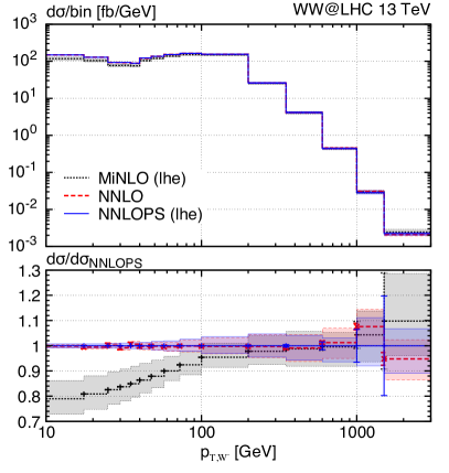
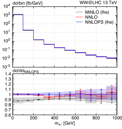
Figure 1: Transverse momenta of the $W^{-}$ boson (left panel) and invariant mass of the leptonic pair coming from the $W^{+}$ boson (right panel), at the $\sqrt{S}=13$ TeV LHC. The red curve is the NNLO prediction (central value with uncertainty), the blue and black ones are the NNLOPS and MiNLO results, respectively (at LHE level, i.e. before parton showering). Figures taken from ref. [7].

In Figure 1 we show two validation plots for $p_{T,W^{-}}$ and $m_{W^{+}}$, where we compare the NNLOPS (and WWJ-MiNLO’) results (before showering) against the NNLO computation, without any fiducial cut. We find excellent agreement between NNLOPS and NNLO, both for an observable used to perform the reweighting ($p_{T,W^{-}}$, left plot), as well as for $m_{W^{+}}$, whose dependence was neglected in the computation of ${\cal W}(\Phi_{B})$: indeed the right plot shows that we exactly reproduce the NNLO result for $m_{W^{+}}$ in the peak region, but also extremely well also quite far in the tail of the distribution. Several other similar results, supporting the validity of the approximations we made, can be found in ref. [7].

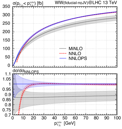
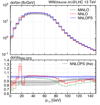
Figure 2: Jet-vetoed cross section (left panel) and transverse momentum of the dilepton system (right panel), at the $\sqrt{S}=13$ TeV LHC, with fiducial cuts. The red curve is the NNLO prediction, the blue and black ones are the NNLOPS and MiNLO results after showering, the green one is the NNLOPS result before parton showering. Figures taken from ref. [7].

Figure 2 shows instead results where the WWJ-MiNLO’ and NNLOPS events have been showered. Here fiducial cuts are also applied. In the left panel one can observe the jet-vetoed cross section, defined as $\sigma(p_{T,j_{1}}<p_{T,j_{1}}^{\rm veto})=\int_{0}^{p_{T,j_{1}}^{\rm veto}}{\rm d}p_{T,j_{1}}\,{{\rm d}\sigma}/{{\rm d}p_{T,j_{1}}}$. The plot shows that the NNLO provides a good description of the jet veto down to $\sim 20$  GeV, supporting the evidence already found in earlier studies. As expected, for lower values of the jet veto the NNLO result becomes unphysical, whereas the NNLOPS one remains well-behaved, due to the all-order resummation of logarithms of the type $\log(M_{WW}/p_{T,j_{1}}^{\rm veto})$. Finally, the right panel of Fig. 2 displays $p_{T,\ell\ell}$, the transverse momentum of the dilepton system. At $p_{T,\ell\ell}\sim 20$  GeV the NNLO curve develops a perturbative instability, due to the presence of a “Sudakov shoulder” [38] caused by the fiducial cut $p_{T}^{\textrm{\scriptsize miss}}{}>20$  GeV. This instability is cured in the NNLOPS (and WWJ-MiNLO’) results. Furthermore, around $p_{T,\ell\ell}{}=100$ GeV a dip appears in the ratio to the showered NNLOPS prediction: this is due to the fact that recoiling effects due to the parton shower can cause a migration of events from one bin to another, and, in some cases, this can also affect leptonic observables.

The computation presented above is now publicly available within the POWHEG BOX framework, and can be used to simulate $W$-boson pair production fully-exclusively at NNLOPS accuracy. It will be interesting to further improve this generator by including the effect of $gg$-induced contributions (for which an NLO+PS study, for the $ZZ$ case, was performed in ref. [39]), as well as to reach NNLOPS accuracy without the need of an explicit reweighting.

References

- [1] S. Höche, F. Krauss, M. Schönherr and F. Siegert, JHEP 1304, 027 (2013)
- [2] F. Cascioli, S. Höche, F. Krauss, P. Maierhöfer, S. Pozzorini and F. Siegert, JHEP 1401, 046 (2014)
- [3] R. Frederix and S. Frixione, JHEP 1212, 061 (2012)
- [4] J. Alwall et al., JHEP 1407, 079 (2014)
- [5] K. Hamilton, P. Nason, C. Oleari and G. Zanderighi, JHEP 1305, 082 (2013)
- [6] K. Hamilton, T. Melia, P. F. Monni, E. Re and G. Zanderighi, JHEP 1609, 057 (2016)
- [7] E. Re, M. Wiesemann and G. Zanderighi, arXiv:1805.09857 [hep-ph].
- [8] K. Hamilton, P. Nason and G. Zanderighi, JHEP 1210, 155 (2012)
- [9] S. Catani, F. Krauss, R. Kuhn and B. R. Webber, JHEP 0111, 063 (2001)
- [10] L. Lonnblad, JHEP 0205, 046 (2002)
- [11] R. Frederix and K. Hamilton, JHEP 1605, 042 (2016)
- [12] S. Carrazza, R. Frederix, K. Hamilton and G. Zanderighi, arXiv:1805.09855 [hep-ph].
- [13] G. Luisoni, P. Nason, C. Oleari and F. Tramontano, JHEP 1310, 083 (2013)
- [14] J. Alwall et al., JHEP 0709, 028 (2007)
- [15] J. M. Campbell, R. K. Ellis, R. Frederix, P. Nason, C. Oleari and C. Williams, JHEP 1207, 092 (2012)
- [16] G. Cullen et al., Eur. Phys. J. C 74, no. 8, 3001 (2014)
- [17] S. Catani and M. Grazzini, Phys. Rev. Lett. 98, 222002 (2007)
- [18] M. Grazzini, S. Kallweit and M. Wiesemann, Eur. Phys. J. C 78, no. 7, 537 (2018)
- [19] T. Gehrmann, M. Grazzini, S. Kallweit, P. Maierhöfer, A. von Manteuffel, S. Pozzorini, D. Rathlev and L. Tancredi, Phys. Rev. Lett. 113, no. 21, 212001 (2014)
- [20] M. Grazzini, S. Kallweit, S. Pozzorini, D. Rathlev and M. Wiesemann, JHEP 1608, 140 (2016)
- [21] M. Grazzini, S. Kallweit, D. Rathlev and A. Torre, Phys. Lett. B 731, 204 (2014)
- [22] M. Grazzini, S. Kallweit and D. Rathlev, JHEP 1507, 085 (2015)
- [23] F. Cascioli et al., Phys. Lett. B 735, 311 (2014)
- [24] M. Grazzini, S. Kallweit and D. Rathlev, Phys. Lett. B 750, 407 (2015)
- [25] M. Grazzini, S. Kallweit, D. Rathlev and M. Wiesemann, Phys. Lett. B 761, 179 (2016)
- [26] M. Grazzini, S. Kallweit, D. Rathlev and M. Wiesemann, JHEP 1705, 139 (2017)
- [27] M. Grazzini, S. Kallweit, D. Rathlev and M. Wiesemann, JHEP 1508, 154 (2015)
- [28] S. Catani and M. H. Seymour, Phys. Lett. B 378, 287 (1996)
- [29] S. Catani and M. H. Seymour, Nucl. Phys. B 485, 291 (1997) Erratum: [Nucl. Phys. B 510, 503 (1998)]
- [30] F. Cascioli, P. Maierhöfer and S. Pozzorini, Phys. Rev. Lett. 108, 111601 (2012)
- [31] F. Buccioni, S. Pozzorini and M. Zoller, Eur. Phys. J. C 78, no. 1, 70 (2018)
- [32] T. Gehrmann, A. von Manteuffel and L. Tancredi, JHEP 1509, 128 (2015)
- [33] K. Hamilton, P. Nason, E. Re and G. Zanderighi, JHEP 1310 (2013) 222
- [34] A. Karlberg, E. Re and G. Zanderighi, JHEP 1409 (2014) 134
- [35] W. Astill, W. Bizoń, E. Re and G. Zanderighi, JHEP 1606 (2016) 154
- [36] W. Astill, W. Bizoń, E. Re and G. Zanderighi, arXiv:1804.08141 [hep-ph].
- [37] J. C. Collins and D. E. Soper, Phys. Rev. D 16, 2219 (1977).
- [38] S. Catani and B. R. Webber, JHEP 9710, 005 (1997)
- [39] S. Alioli, F. Caola, G. Luisoni and R. Röntsch, Phys. Rev. D 95, no. 3, 034042 (2017)