Satellite-based quantum steering under the influence of spacetime curvature of the Earth

Abstract

Spacetime curvature of the Earth deforms wavepackets of photons sent from the Earth to satellites, thus influencing the quantum state of light. We show that Gaussian steering of photon pairs, which are initially prepared in a two-mode squeezed state, is affected by the curved spacetime background of the Earth. We demonstrate that quantum steerability of the state increases for a specific range of height $h$ and then gradually approaches a finite value with further increasing height of the satellite’s orbit. Comparing with the peak frequency parameter, the Gaussian steering changes more for different squeezing parameters, while the gravitational frequency effect leads to quantum steering asymmetry between the photon pairs. In addition, we find that the influence of spacetime curvature on the steering in the Kerr spacetime is very different from the non-rotating case because special relativistic effects are involved.

I Introduction

Einstein-Podolsky-Rosen (EPR) steering, which describes how the state of one subsystem in an entangled pair is manipulated by local measurements performed on the other part, was proposed by Schrödinger in 1935 E.P.C ; E.P.C1 . The EPR steering differs from both entanglement and the Bell nonlocality, because it has inherent asymmetric features. Therefore, the EPR steering has potential applications in the one-side device-independent quantum key distribution CBEG . Recently, quantum steering and its asymmetry have been theoretically studied HMW ; Skrzypczyk ; Kocsis ; Adesso2015 ; steering3 ; steering4 ; MWZZ ; steering5 ; SLCC and experimentally demonstrated Walborn ; steering2 ; Bowles ; VHTE ; VHTSS ; Handchen ; BWSR ; SKMJ ; DJSS ; TEVH ; Xiao2017 ; SWNW in different quantum systems. However, little is known about behaviors of quantum steering in relativistic settings. Most recently, Navascues and Perez-Garcia studied quantum steering between space-like separated parties in the frame of algebraic quantum field theory steeringrqi . In addition, more attention has been given to the dynamics of quantum steering under the influence of the dynamical Casimir effect steeringrqi1 , the Hawking radiation steeringrqi2 , and relativistic motions steeringrqi3 .

Since a realistic quantum system cannot be prepared and transmitted in a curved spacetime without any gravitational and relativistic effects, the study of quantum steerability in a relativistic framework is necessary. Such studies are of practical and fundamental importance to understand the influence of gravitational effects on the steerability-type quantum resource when the parties involved are located at large distances in the curved space time DEBA ; DEBT ; satellite1 ; satellite2 ; kerr . It has been shown that the curved background spacetime of the Earth affects the running of quantum clocks Alclock , is employed as witnesses of general relativistic proper time in laser interferometric Zych , and influences the implementation of quantum metrology MADE ; MADE2 in satellite-based setups. Furthermore, Kish and Ralph found that there would be inevitable losses of quantum resources in the estimation of the Schwarzschild radius SPK . We studied how the curved background spacetime of the Earth influences the satellite-based quantum clock synchronization wangsyn . Most recently, an experimental test of photonic entanglement in an accelerated setting was realized RQI8 , where a genuine quantum state of entangled photon pairs was exposed to different accelerations.

In this work, we present a quantitative investigation of Gaussian quantum steerability for correlated photon pairs which are initially prepared in a two-mode squeezed state in the curved background spacetime of the Earth. We assume that one of entangled photons is sent to Alice (at the Earth station) and the other propagates to Bob (at the satellite). During this propagation, the photons’ wave-packet will be deformed by the curved background spacetime of the Earth, and these deformations effects on the quantum state of the photons can be modeled as a lossy quantum channel MANI ; wangsyn . Since the initial state is Gaussian and the transformations involved are linear and unitary, we can restrict our state to the Gaussian scenarios and employ the covariance matrix formalism. We calculate the Gaussian quantum steering from Alice to Bob, which quantifies to what extent Bob’s mode can be steered by Alice’s measurements. We also discuss Gaussian quantum steering from Bob to Alice to verify the asymmetric property of steerability in the curved spacetime.

This work is organized as follows. In section II, we introduce the quantum field theory of a massless uncharged bosonic field which propagates from the Earth to a satellite. In section III, we briefly introduce the definition and measure of the bipartite Gaussian quantum steering. In section IV, we show a scheme to test quantum steering between the Earth and satellites and study the behaviors of quantum steering in the curved spacetime. The last section is devoted to a brief summary. Throughout the whole paper we employ the natural units $G=c=\hbar=1$.

II Light wave-packets propagating in the curved space-time

In this section we will describe the propagation of photons from the Earth to satellites under the influence of the Earth’s gravity DEBT . The Earth’s spacetime can be approximately described by the Kerr metric Visser . For the sake of simplicity, our work will be constrained to the equatorial plane $\theta=\frac{\pi}{2}$. The reduced metric in Boyer-Lindquist coordinates $(t,r,\phi)$ reads Visser

$$ds^{2}= \,-\Big{(}1-\frac{2M}{r}\Big{)}dt^{2}+\frac{1}{\Delta}dr^{2}$$

$$\,+\Big{(}r^{2}+a^{2}+\frac{2Ma^{2}}{r}\Big{)}d\phi^{2}-\frac{4Ma}{r}dt\,d\phi,$$ (1)

$$\Delta= \,1-\frac{2M}{r}+\frac{a^{2}}{r^{2}},$$ (2)

where $M$, $r$, $J$, $a=\frac{J}{M}$ are the mass, radius, angular momentum and Kerr parameter of the Earth, respectively.

A photon is sent from Alice on Earth’s surface to Bob at time $\tau_{A}$, Bob will receive this photon at $\tau_{B}=\Delta\tau+\sqrt{f(r_{B})/f(r_{A})}\tau_{A}$ in his own reference frame, where $f(r_{A})=1-\frac{r_{S}}{r_{A}}$ and $f(r_{B})=1-\frac{r_{S}}{r_{B}}$. Here $r_{S}=2M$ is the Schwarzschild radius of the Earth and $\Delta\tau$ is the propagation time of the light from the Earth to the satellite by taking curved effects of the Earth into account. In general, a photon can be modeled by a wave packet of excitations of a massless bosonic field with a distribution $F^{(K)}_{\Omega_{K,0}}$ of mode frequency $\Omega_{K}$ and peaked at $\Omega_{K,0}$ ULMQ ; TGDT , where $K=A,B$ denote the modes in Alice’s or Bob’s reference frames, respectively. The annihilation operator of a photon for an observer far from Alice or Bob takes the form

$$a_{\Omega_{K,0}}(t_{K})=\int_{0}^{+\infty}d\Omega_{K}e^{-i\Omega_{K}t_{K}}F^{(K)}_{\Omega_{K,0}}(\Omega_{K})a_{\Omega_{K}}.$$ (3)

Alice’s and Bob’s operators in Eq. (3) can be used to describe the same optical mode in different altitudes. By considering the curved spacetime of the Earth, the wave packet received is modified. The relation between $a_{\Omega_{A}}$ and $a_{\Omega_{B}}$ was discussed in DEBT ; DEBA ; wangsyn , and can be used to calculate the relation between the frequency distributions $F^{(K)}_{\Omega_{K,0}}$ of the photons before and after the propagation DEBT ; DEBA ; wangsyn

$$F^{(B)}_{\Omega_{B,0}}(\Omega_{B})=\sqrt[4]{\frac{f(r_{B})}{f(r_{A})}}F^{(A)}_{\Omega_{A,0}}\left(\sqrt{\frac{f(r_{B})}{f(r_{A})}}\Omega_{B}\right).$$ (4)

From Eq. (4), we can see that the effect induced by the curved spacetime of the Earth cannot be simply corrected by a linear shift of frequencies. Therefore, it may be challenging to compensate the transformation induced by the curvature in realistic implementations.

Indeed, such a nonlinear gravitational effect is found to influence the fidelity of the quantum channel between Alice and Bob DEBT ; DEBA ; wangsyn . It is always possible to decompose the mode $\bar{a}^{\prime}$ received by Bob in terms of the mode $a^{\prime}$ prepared by Alice and an orthogonal mode $a_{\bot}^{\prime}$ (i.e. $[a^{\prime},a_{\bot}^{\prime\dagger}]=0$) PPRW

$$\bar{a}^{\prime}=\Theta a^{\prime}+\sqrt{1-\Theta^{2}}a_{\bot}^{\prime},$$ (5)

where $\Theta$ is the wave packet overlap between the distributions $F^{(B)}_{\Omega_{B,0}}(\Omega_{B})$ and $F^{(A)}_{\Omega_{A,0}}(\Omega_{B})$,

$$\Theta:=\int_{0}^{+\infty}d\Omega_{B}\,F^{(B)\star}_{\Omega_{B,0}}(\Omega_{B})F^{(A)}_{\Omega_{A,0}}(\Omega_{B}),$$ (6)

and we have $\Theta=1$ for a perfect channel. From this expression we can see that the spacetime curvature of the Earth would affect the the fidelity $\mathcal{F}=|\Theta|^{2}$ as well as the quantum resource of EPR steering.

We assume that Alice employs a real normalized Gaussian wave packet

$$F_{\Omega_{0}}(\Omega)=\frac{1}{\sqrt[4]{2\pi\sigma^{2}}}e^{-\frac{(\Omega-\Omega_{0})^{2}}{4\sigma^{2}}},$$ (7)

with wave packet width $\sigma$. In this case the overlap $\Theta$ is given by (6) where we have extended the domain of integration to all the real axis. We note that the integral should be performed over strictly positive frequencies. However, since $\Omega_{0}\gg\sigma$, it is possible to include negative frequencies without affecting the value of $\Theta$. Using Eqs. (3) and (7) one finds that DEBT ; DEBA ; wangsyn

$$\Theta=\sqrt{\frac{2}{1+(1+\delta)^{2}}}\frac{1}{1+\delta}e^{-\frac{\delta^{2}\Omega_{B,0}^{2}}{4(1+(1+\delta)^{2})\sigma^{2}}},$$ (8)

where the new parameter $\delta$ quantifying the shifting is defined by

$$\delta=\sqrt[4]{\frac{f(r_{A})}{f(r_{B})}}-1=\sqrt{\frac{\Omega_{B}}{\Omega_{A}}}-1.$$ (9)

The expression for $\frac{\Omega_{B}}{\Omega_{A}}$ in the equatorial plane of the Kerr spacetime has been shown in kerr

$$\frac{\Omega_{B}}{\Omega_{A}}=\frac{1+\epsilon\frac{a}{r_{B}}\sqrt{\frac{M}{r_{B}}}}{C\sqrt{1-3\frac{M}{r_{B}}+2\epsilon\frac{a}{r_{B}}\sqrt{\frac{M}{r_{B}}}}},$$ (10)

where $C=[1-\frac{2M}{r_{A}}(1+2a{\omega})+\big{(}r^{2}_{A}+a^{2}-\frac{2Ma^{2}}{r_{A}}\big{)}{\omega}^{2}]^{-\frac{1}{2}}$ is the normalization constant, $\omega$ is the Earth’s equatorial angular velocity and $\epsilon=\pm 1$ stand for the direct of orbits (i.e., when $\epsilon=+1$ for the satellite co-rotates with the Earth). In the Schwarzschild limit $a,\omega\rightarrow 0$, Eq. (10) coincides to the result found in DEBT , which is

$$\frac{\Omega_{B}}{\Omega_{A}}=\sqrt{\frac{1-\frac{2M}{r_{A}}}{1-\frac{3M}{r_{B}}}}.$$ (11)

Noticing that $(r_{A}\omega)^{2}>a\omega$, therefore we can retain second order terms in $r_{A}\omega$. Expanding Eq. (10) we obtain the following perturbative expression for $\delta$. This perturbative result does not depend on whether the Earth and the satellite are co-rotating or not

$$\delta = \delta_{Sch}+\delta_{rot}+\delta_{h}$$

$$= \frac{1}{8}\frac{r_{S}}{r_{A}}\big{(}\frac{1-2\frac{h}{r_{A}}}{1+\frac{h}{r_{A}}}\big{)}-\frac{(r_{A}\omega)^{2}}{4}-\frac{(r_{A}\omega)^{2}}{4}\big{(}\frac{3}{4}\frac{r_{S}}{r_{A}}-\frac{4Ma}{\omega r_{A}^{3}}\big{)},$$

where $h=r_{B}-r_{A}$ is the height between Alice and Bob, $\delta_{Sch}$ is the first order Schwarzschild term, $\delta_{rot}$ is the lowest order rotation term and $\delta_{h}$ denotes all higher order correction terms. If the parameter $\delta=0$ (the satellite moves at the height $h\simeq\frac{r_{A}}{2}$), we have $\Theta=1$. That is to say, the received photons at this height will not experience any frequency shift, and the effects of gravity of the Earth and the effects of special relativity completely compensates each other.

III Gaussian quantum steering

In this section we briefly review the measurement of quantum steering for a general two-mode Gaussian state $\rho_{AB}$. The character of a bipartite Gaussian state ${\rho_{AB}}$ can be described by its covariance matrix (CM)

$$\sigma_{AB}=\left({\begin{array}[]{*{20}{c}}A&C\\ {{C^{\sf T}}}&B\\ \end{array}}\right),$$ (12)

with elements ${\sigma_{ij}}=\text{Tr}\big{[}{{{\{{{{\hat{R}}_{i}},{{\hat{R}}_{j}}}\}}_{+}}\ {\rho_{AB}}}\big{]}$. Here the submatrices $A$ and $B$ are the CMs correspoding to the reduced states of $A$’s and $B$’s subsystems, respectively. The bona fide condition should be satisfied for a physical CM, which is

$${\sigma_{AB}}+i\,({\Omega_{A}}\oplus{\Omega_{B}})\geq 0.$$ (13)

Let us continue by giving the definition of steerability. For a bipartite state, it is steerable from $A$ to $B$ iff it is not possible for every pair of local observables $R_{A}\in\mathcal{M}_{A}$ on $A$ and $R_{B}$ (arbitrary) on $B$, with respective outcomes $r_{A}$ and $r_{B}$, to express the joint probability as HMWS $P\left({{r_{A}},{r_{B}}|{R_{A}},{R_{B}},{\rho_{AB}}}\right)=\sum\limits_{\lambda}{{\wp_{\lambda}}}\,\wp\left({{r_{A}}|{R_{A}},\lambda}\right)P\left({{r_{B}}|{R_{B}},{\rho_{\lambda}}}\right)$. That is to say, there exists at least one measurement pair between $R_{A}$ and $R_{B}$ that can violate this expression when ${\wp_{\lambda}}$ is fixed across all measurements. Here ${\wp_{\lambda}}$ and $\wp\left({{r_{A}}|{R_{A}},\lambda}\right)$ are arbitrary probability distributions and $P\left({{r_{B}}|{R_{B}},{\rho_{\lambda}}}\right)$ is a probability distribution restricted to the extra condition of being evaluated on a quantum state $\rho_{\lambda}$. It has been proven that a necessary and sufficient condition for Gaussian $A\to B$ steerability is iff the condition

$${\sigma_{AB}}+i\,({0_{A}}\oplus{\Omega_{B}})\geq 0,$$ (14)

is violated HMWS . To quantify how much a bipartite Gaussian state with CM $\sigma_{AB}$ is steerable (by Gaussian measurements on Alice’s side), the following quantity has been performed IKAR

$${\cal G}^{A\to B}(\sigma_{AB}):=\max\bigg{\{}0,\,-\sum_{j:\bar{\nu}^{B}_{j}<1}\ln(\bar{\nu}^{B}_{j})\bigg{\}}\,,$$ (15)

where $\bar{\nu}^{B}_{j}$ are the symplectic eigenvalues of the Schur complement of $A$ in the covariance matrix $\sigma_{AB}$. By defining the Schur complement $\det{\sigma_{AB}}=\det{A}\det{M^{B}_{\sigma}}$ and employing the Rényi-$2$ entropy, Eq. (15) can be written as

$${\cal G}^{A\to B}(\sigma_{AB}) = \max\big{\{}0,\,\frac{1}{2}\ln{\frac{\det A}{\det\sigma_{AB}}}\big{\}}$$ (16)

$$= \max\big{\{}0,\,{\cal S}(A)-{\cal S}(\sigma_{AB})\big{\}}\,,$$

where the Rényi-$2$ entropy ${\cal S}$ reads ${\cal S}(\sigma)=\frac{1}{2}\ln(\det\sigma)$ renyi for a Gaussian state with CM $\sigma$. However, unlike quantum entanglement, quantum steering is asymmetric IKAR . To obtain the measurement of Gaussian steering $B\rightarrow A$, one can swap the roles of $A$ and $B$ and get an expression like Eq. (16).

IV The influence of gravitational effects on quantum steerability and entanglement

In this section we propose a scheme to test large distance quantum steering between the Earth and satellites and discuss how quantum steerability is affected by the curved spacetime of the Earth. Firstly, we consider a pair of entangled photons which are initially prepared in a two-mode squeezed state with modes $b_{1}$ and $b_{2}$ at the ground station. Then we send one photon with mode $b_{1}$ to Alice. The other photon in mode $b_{2}$ propagates from the Earth to the satellite and is received by Bob. Due to the curved background spacetime of the Earth, the wave packet of photon with mode $b_{2}$ is deformed. Finally, one can test how the quantum state of Alice’s photon is manipulated by local Gaussian measurements performed by Bob at the satellite and verifies the quantum steerability from $b_{2}$ to $b_{1}$, and vice versa.

Considering that Alice receives the mode $b_{1}$ and Bob receives the mode $b_{2}$ at different satellite orbits, we should take the curved spacetime of the Earth into account. As discussed in DEBT ; DEBA ; wangsyn , the influence of the Earth’s gravitational effect can be modeled by a beam splitter with orthogonal modes $b_{1\bot}$ and $b_{2\bot}$. The covariance matrix of the initial state is given by

$$\Sigma^{b_{1}b_{2}b_{1\bot}b_{2\bot}}_{0}=\left(\begin{array}[]{cc}\tilde{\sigma}(s)&0\\ 0&I_{4}\end{array}\right),$$ (17)

where ${I}_{4}$ denotes the $4\times 4$ identity matrix and $\tilde{\sigma}{(s)}$ is the covariance matrix of the two-mode squeezed state

$$\tilde{\sigma}(s)=\left(\begin{array}[]{cc}\cosh{(2s)}{I}_{2}&\sinh{(2s)}\sigma_{z}\\ \sinh(2s)\sigma_{z}&\cosh{(2s)}{I}_{2}\end{array}\right),$$ (18)

where $\sigma_{z}$ is Pauli matrix and $s$ is the squeezing parameter. The effect induced by the curved spacetime of the Earth on Bob’s mode $b_{2}$ can be model as a lossy channel, which is described by the transformation DEBT ; DEBA ; wangsyn

$$\bar{b}_{2} = \Theta_{2}\,b_{2}+\sqrt{{1-\Theta_{2}^{2}}}b_{2\bot},$$ (19)

while the mode $b_{1}$ received by Alice is unaffected because Alice stays at the ground station. This process can be represented as a mixing (beam splitting ) of modes $b_{1}(b_{2})$ and $b_{1\bot}(b_{2\bot})$. Therefore, for the entire state, the symplectic transformation can be encoded into the Bogoloiubov transformation

$$S=\left(\begin{array}[]{cccc}{I}_{2}&0&0&0\\ 0&\Theta_{2}{I}_{2}&0&\sqrt{1-\Theta_{2}^{2}}{I}_{2}\\ 0&0&-{I}_{2}&0\\ 0&\sqrt{1-\Theta_{2}^{2}}{I}_{2}&0&-\Theta_{2}{I}_{2}\end{array}\right).$$

The final state $\Sigma^{b_{1}b_{2}b_{1\bot}b_{2\bot}}$ after the transformation is $\Sigma^{b_{1}b_{2}b_{1\bot}b_{2\bot}}=S\,\Sigma_{0}^{b_{1}b_{2}b_{1\bot}b_{2\bot}}\,S^{T}$. Then we trace over the orthogonal modes $b_{1\bot},b_{2\bot}$ and obtain the covariance matrix $\Sigma^{b_{1}b_{2}}$ for the modes $b_{1}$ and $b_{2}$ after the propagation

$$\Sigma^{b_{1}b_{2}}=\left(\begin{array}[]{cc}(1+2\sinh^{2}s){I}_{2}&\sinh{(2s)}\,\Theta_{2}\,\sigma_{z}\\ \sinh{(2s)}\,\Theta_{2}\,\sigma_{z}&(1+2\sinh^{2}s\,\Theta_{2}^{2})\,{I}_{2}\end{array}\right).$$ (20)

The form of the two-mode squeezed state under the influence of the effects of gravity of the Earth is given by Eq. (20). Then employing the measurement of Gaussian steering, we obtain an specific mathematic expression of the mode $b_{1}\rightarrow b_{2}$ Gaussian steering under the curved spacetime of the Earth

$${\cal G}^{b_{1}\to b_{2}} = \mbox{$\max\big{\{}0,\,\ln{\frac{1+2\sinh^{2}(2s)}{1+2(1-\Theta_{2}^{2})\sinh^{2}s}}\big{\}}$}.$$ (21)

We notice that the wave packet overlap $\Theta$ in the above equation is determined by the parameters $\delta$, $\sigma$ and $\Omega_{B,0}$. Since the Schwarzschild radius of the Earth is $r_{s}=9$ mm, we have $\delta\sim-\frac{1}{2}(\frac{r_{s}}{r_{B}}-\frac{r_{s}}{r_{A}})\sim 10^{-10}$. Here we consider a typical PDC source with a wavelength of 598 nm (corresponding to the peak frequency $\Omega_{B,0}=500$ THz) and Gaussian bandwidth $\sigma=1$MHz [48, 49]. Under these constraints, $\delta\ll(\frac{\Omega_{B,0}}{\sigma})^{2}\ll 1$ is satisfied. Therefore, the wave packet overlap $\Theta$ can be expand by the parameter $\delta$. Then we obtain $\Theta\sim 1-\frac{\delta^{2}\Omega_{B,0}^{2}}{8\sigma^{2}}$ by keeping the second order terms. The Eq. (21) has following form in the second order of perturbation for the parameter $\delta$

$${\cal G}^{b_{1}\to b_{2}}\simeq\max\{0,{\cal G}_{0}-\frac{\delta^{2}\Omega_{B,0}^{2}}{2\sigma^{2}}\sinh^{2}(s)\},$$ (22)

where higher order contributions are neglected. To ensure the validity of perturbative expansion, we should estimate the values of the last term in Eq. (22). Considering $\frac{\delta^{2}\Omega^{2}_{B,0}}{2\sigma^{2}}\sim 1.25\times 10^{-7}$, we find that even if the value of the squeezing parameter is $s\ll 7.6$ (corresponding to $\sinh^{2}(s)\ll 10^{6}$), the perturbative expansion is valid. Therefore, we can safely prelimit the value of the squeezing parameter as $s<3$ hereafter. In the case of flat spacetime, this expression reduces to ${\cal G}_{0}:=\ln{[1+2\sinh^{2}(2s)]}$. As showed in Eq. (22), the Gaussian steering $b_{1}\to b_{2}$ not only depends on the squeezing parameter, the peak frequency, and the Gaussian bandwidth, but also the height of the orbiting satellite. This means that the curved spacetime of the Earth will influence the $b_{1}\to b_{2}$ steerability because the parameter $\delta$ contains the height $h$ of the satellite. It is clear that $\delta$ approaches to a constant value when the height $h\rightarrow\infty$ and the squeezing parameter $s$ is a fixed value. Therefore, quantum steering ${\cal G}^{b_{1}\to b_{2}}$ also becomes a constant.

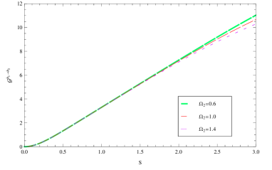
Figure 1: (Color online) The Gaussian steering ${\cal G}^{b_{1}\to b_{2}}$ of two-mode squeezed state as a function of the squeezing parameter $s$ for different peak frequencies, $\Omega_{2}=0.6$ (green dashed line), $\Omega_{2}=1$ (red dashed line) and $\Omega_{2}=1.4$ (violet dotted line), respectively. The orbit height of the satellite and the Gaussian bandwidth are fixed as $h=20000$km and $\sigma=1$.

For convenience, we will work with dimensionless quantities by rescaling the peak frequency and the Gaussian bandwidth

$$\Omega\rightarrow\tilde{\Omega}\equiv\frac{\Omega}{\Omega_{B,0}},\sigma\rightarrow\tilde{\sigma}\equiv\frac{\sigma}{\sigma_{0}},$$ (23)

where $\Omega_{B,0}=500$THz and $\sigma_{0}=1$ MHz. For simplicity, we abbreviate the dimensionless parameter $\tilde{\Omega}$ as $\Omega_{2}$ and abbreviate $\tilde{\sigma}$ as $\sigma$, respectively.

In Fig. (1) we plot the Gaussian steering ${\cal G}_{b_{1}\to b_{2}}$ as a function of the squeezing parameter $s$ for the fixed orbit height $h=20000$ km and Gaussian bandwidth $\sigma=1$. We can see that quantum steering monotonically increases with the increase of the squeezing parameter $s$. It is also shown that, comparing with the peak frequency parameter, the Gaussian steering $\mathcal{G}^{b_{1}\to b_{2}}$ changes more for different squeezing parameters, which indicates that the initial quantum resource plays a more important role in the quantum steering.

The Gaussian steering ${\cal G}_{b_{1}\to b_{2}}$ in terms of the orbit height $h$ and the Gaussian bandwidth $\sigma$ for the fixed values $s=1$ and $\Omega_{2}=1$ has been shown in Fig. (2). We can see that the quantum steerability ${\cal G}_{b_{1}\to b_{2}}$ decreases with increasing the Gaussian bandwidth $\sigma$. In addition, comparing with the squeezing parameter, the Gaussian steering is not easy to change with changing orbit height parameter and Gaussian bandwidth. This allows us to choose appropriate physical parameters and perform more reliable quantum steering tasks between the Earth to a satellite.

Figure 2: (Color online) The Gaussian steering ${\cal G}_{b_{1}\to b_{2}}$ in terms of the orbit height $h$ and the Gaussian bandwidth $\sigma$, for the fixed values $s=1$ and $\Omega_{2}=1$.

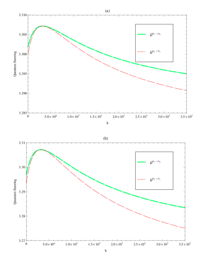
Figure 3: (Color online). The Gaussian steering ${\cal G}^{b_{1}\to b_{2}}$ (green lines) and ${\cal G}^{b_{2}\to b_{1}}$ (orange lines) as functions of the height between Alice and Bob under the influence of the Earth’s gravity. Here the Gaussian bandwidth of the initial state is fixed as $\sigma=1$, the dimensionless peak frequencies of the mode $b_{2}$ are fixed as (a) $\Omega_{2}=0.6$, (b) $\Omega_{2}=1$, and the squeezing parameter is $s=1$.

One of the most distinguishable properties of quantum steering is its asymmetry, which has been recently experimentally demonstrated in flat spacetime VHTE ; VHTSS . To understanding this properties in the curved spacetime, we also calculate the steerability ${\cal G}^{b_{2}\to b_{1}}$, which is

$${\cal G}^{b_{2}\to b_{1}} = \mbox{$\max\big{\{}0,\,\ln{\frac{1+2\sinh^{2}(2s)\Theta_{2}^{2}}{1+2(1-\Theta_{2}^{2})\sinh^{2}s}}\big{\}}$},$$ (24)

Similarly, this equation can be rewritten in its perturbative expansion form as

$${\cal G}^{b_{2}\to b_{1}}\simeq\max{\{0,\,{\cal G}_{0}-\frac{\delta^{2}\Omega_{B,0}^{2}}{2\sigma^{2}}(\sinh^{2}{(s)}+\frac{\sinh^{2}{(2s)}}{\cosh{(4s)}}})\}.$$ (25)

This equation gives us a quantitative way to evaluate the contributions of the curved background spacetime of the Earth to the steering for the $b_{2}\to b_{1}$ scenario, when the satellites are far away to the Earth. It is clearly shown that ${\cal G}^{b_{2}\to b_{1}}$ is equal to ${\cal G}_{0}$ when the $\delta\rightarrow 0$, which means that the effect induced by the curved background spacetime of the Earth vanishes in this limit.

The typical distance between the ground station and the geostationary satellite is about $3.6\times 10^{4}$km, which yields the height $r_{B}=4.237\times 10^{4}$ km for the satellite. Since the height of current GPS (Global Position System) satellites is $r_{B}\approx 2.7\times 10^{4}$km. For this distance the influence of relativistic disturbance of the spacetime curvature on quantum steerability cannot be ignored for the quantum information tasks at current level technology satellite1 ; satellite2 ; MJAG . Hence, in this work the plotting range of the satellite height will be constrained to geostationary satellites height.

In Fig. (3), we plot the quantum steerability ${\cal G}^{b_{1}\to b_{2}}$, as well as ${\cal G}^{b_{2}\to b_{1}}$ of the final state as a function of the height $h$. The plot range is limited to geostationary Earth orbits $r_{B}(GEO)=r_{A}+35784$ km. Here, the range of peak frequency parameter $\Omega_{2}$ is fixed from $0.6$ to $1$ to satisfy $\delta\ll(\frac{\delta\Omega_{2}}{\sigma})^{2}\ll 1$. It is shown that both the $b_{1}\rightarrow b_{2}$ and $b_{2}\rightarrow b_{1}$ steering increase for a specific range of height parameter $h$ and then gradually approach to a finite value with increasing $h$. This is because the total frequency shift in Eq. (10) both includes the Schwarzschild term and the rotation term. The parameter $\delta$ in the Kerr spacetime is $\delta=\frac{1}{8}\frac{r_{S}}{r_{A}}\big{(}\frac{1-2\frac{h}{r_{A}}}{1+\frac{h}{r_{A}}}\big{)}$ which is different from the Schwarzschild case $\delta_{Sch}^{{}^{\prime}}=-\frac{r_{S}}{4r_{A}}\frac{h}{(r_{A}+h)}$ DEBT ; DEBA since special relativistic effects are involved kerr . When the satellite moves at the height $h=\frac{r_{A}}{2}$, the Schwarzschild term $\delta_{Sch}$ vanishes and photons received on satellites will generate a very small frequency shift dominated by special relativistic effects, therefore the lowest order rotation term $\delta_{rot}$ needs to be considered. In addition, we can see that whatever ${\cal G}^{b_{1}\to b_{2}}$ or ${\cal G}^{b_{2}\to b_{1}}$ both reduce with increasing $h$ after reaches the peak. That’s why we say the gravitational frequency shift effect is a lossy channel. This losing degree of quantum steering depends on the dimensionless peak frequency of mode $b_{2}$, which means that this lossy channel not only depends on curvature of the Earth.

In fact, the peak value of quantum steering indicates the fact that the photon’s frequency received by satellites experiences a transformation from blue-shift to red-shift, which causes the Gaussian steering between the photon pairs to increase first and then to reduce with increasing height kerr . In the Schwarzschild limit $a,\omega_{A}\to 0$, the frequency shift simplifies to $\frac{\Omega_{B}}{\Omega_{A}}=\sqrt{\frac{1-\frac{2M}{r_{A}}}{1-\frac{3M}{r_{B}}}},$ from which we can see that the received photon’s frequency on satellites do not experience any frequency shift at $h=\frac{r_{A}}{2}$. On the other hand, the frequency of photon received at orbits with height $h<\frac{r_{A}}{2}$ will experience blue-shift, while the frequencies of photons received at height $h>\frac{r_{A}}{2}$ experience red-shift. For this reason, the photons experience different frequency shifts when the satellite locates at different heights in the Kerr spacetime. Therefore, the Gaussian steering increases at the beginning, reaches the peak value (corresponds to the satellite at the heights $h\approx\frac{r_{A}}{2}$, i.e. the parameter $\delta=0$ ), and then decreases with increasing height.

To check the asymmetric degree of steerability under the Earth’s spacetime curvature, we calculate the Gaussian steering asymmetry

$${\cal G}^{\Delta}=|{\cal G}^{b_{1}\to b_{2}}-{\cal G}^{b_{2}\to b_{1}}|,$$ (26)

and plot it as a function of the peak frequency $\Omega_{2}$ and the height $h$ of the satellite in Fig. (4). This allows us to have a better understanding of how the peak frequency $\Omega_{2}$ and the Earth’s gravitation affect steering asymmetry. It is shown that the ${\cal G}^{\Delta}$ is close to zero, i.e., the steerability is almost symmetric when the height parameter $h\to 0$ and the peak frequency $\Omega_{2}\to 0$ because ${\cal G}^{b_{1}\to b_{2}}\approx{\cal G}^{b_{2}\to b_{1}}$ in these two cases. In addition, the steering asymmetry monotonically increases with increasing orbit height $h$ of the satellite. The physical support behind this is that gravitational field would reduce quantum resource MAK , and the effect of gravitational field on different directions of steering is different steeringrqi2 . Furthermore, it is not difficult to infer that if the gravitation is strong enough or Bob is close to the horizon of a black hole, the gravitational frequency should lead to completely asymmetry: Alice can steer Bob but Bob cannot steer Alice at all.

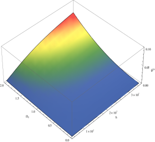
Figure 4: (Color online) The Gaussian steering asymmetry ${\cal G}^{\Delta}$ as a function of the height $h$ of the satellite and the peak frequency $\Omega_{2}$ of mode $b_{2}$. The Gaussian bandwidth and the squeezing parameter are fixed as $\sigma=1$ and $s=1$, respectively.

V Conclusions

In conclusion, we have studied Gaussian steering for a two-mode Gaussian state when one of the modes propagates from the ground to satellites. We found that the frequency shift induced by the curved spacetime of the Earth reduces the quantum correlation of the steerability between the photon pairs when one of the entangled photons is sent to the Earth station and the other photon is sent to the satellite. In addition, the influence of spacetime curvature on the steering in the Kerr spacetime is very different from the non-rotation case because special relativistic effects are involved. We also found that Gaussian steering is easier to change with the initial squeezing parameter than the gravitational effect and other parameters. Although the gravitational effect of the Earth is small, it will lead to the Gaussian steering asymmetry between the photon pairs. This is because the influence of gravitational field on the steering of the downlink setup is stronger than the effect of gravitational field on the steering of the uplink setup, which results in the increase of quantum steering asymmetry. Therefore, we can conclude that the effects induced by the curved spacetime of the Earth will generate quantum steering asymmetry. Finally, the peak value is found to be a critical point which indicates the received photons experience a transformation from blue-shift to red-shift. According to the equivalence principle, the effects of acceleration are equivalence with the effects of gravity, our results could be in principle apply to dynamics of quantum steering under the influence of acceleration. Since realistic quantum systems will always exhibit gravitational and relativistic features, our results should be significant both for giving more advices to realize quantum information protocols such as quantum key distribution from Earth to satellites and for a general understanding of quantum steering in relativistic quantum systems.

- (1) E. Schrödinger, Proc. Camb. Phil. Soc 1935, 31, 553.
- (2) E. Schrödinger, Proc. Camb. Phil. Soc 1936, 32, 446.
- (3) C. Branciard, E. Cavalcanti, S. Walborn, V. Scarani, and H. Wiseman, Phys. Rev. A 2012, 85, 010301.
- (4) H. Wiseman, S. Jones, and A. Doherty, Phys. Rev. Lett 2007, 98, 140402.
- (5) P. Skrzypczyk, M. Navascués, and D. Cavalcanti, Phys. Rev. Lett 2014, 112, 180404.
- (6) Q. He, Q. Gong, and M. Reid, Phys. Rev. Lett 2015, 114 060402.
- (7) I. Kogias, A. Lee, S. Ragy, and G. Adesso, Phys. Rev. Lett 2015, 114, 060403.
- (8) M. Marciniak, A. Rutkowski, Z. Yin, M. Horodecki, and R. Horodecki, Phys. Rev. Lett 2015, 115, 170401.
- (9) Q. He, L. Rosales-Zárate, G. Adesso, and M. Reid, Phys. Rev. Lett 2015, 115, 180502.
- (10) M. Wang, Z. Qin, and X. Su, Phys. Rev. A 2017, 95, 052311.
- (11) A. Sainz, N. Brunner, D. Cavalcanti, P. Skrzypczyk, and T. Vertesi, Phys. Rev. Lett 2015, 115, 190403.
- (12) S. Chen, C. Budroni, Y. Liang, and Y. Chen Phys. Rev. Lett 2016, 116, 240401.
- (13) S. Walborn, A. Salles, R. Gomes, F. Toscano, and P. Souto-Ribeiro, Phys. Rev. Lett 2011, 106, 130402.
- (14) C. Li, K. Chen, Y. Chen, Q. Zhang, Y. Chen, and J. Pan, Phys. Rev. Lett 2015, 115, 010402.
- (15) J. Bowles, T. Vértesi, M. Quintino, and N. Brunner, Phys. Rev. Lett 2014, 112, 200402.
- (16) V. Hndchen, T. Eberle, S. Steinlechner, A. Samblowski, T. Franz, R. Werner and R. Schnabel, Nat. Photon 2012, 6, 596.
- (17) S. Wollmann, N. Walk, A. Bennet, H. Wiseman, and G. Pryde, Phys. Rev. Lett 2016, 116, 160403.
- (18) T. Guerreiro, F. Monteiro, A. Martin, J. Brask, T. Vértesi, B. Korzh, M. Caloz, F. Bussires, V. Verma, A. Lita, R. Mirin, S. Nam, F. Marsilli, M. Shaw, N. Gisin, N. Brunner, H. Zbinden, and R. Thew, Phys. Rev. Lett 2016, 117, 070404.
- (19) B. Wittmann, S. Ramelow, F. Steinlechner, N. Langford, N. Brunner, H. Wiseman, R. Ursin, and A. Zeilinger, New Journal of Physics 2012, 14, 053030.
- (20) S. Kocsis, M. Hall, A. Bennet, and G. Pryde, Nat. Commun 2015, 6, 5886.
- (21) D. Saunders, S. Jones, H. Wiseman, and G. Pryde, Nat. Phys 2010, 6, 845.
- (22) T. Eberle, V. Hndchen, J. Duhme, T. Franz, R. F-Werner, and R. Schnabel, Phys. Rev. A 2011, 83, 052329.
- (23) Y. Xiao, X. Ye, K. Sun, J. Xu, C. Li, and G. Guo, Phys. Rev. Lett 2017, 118, 140404.
- (24) S. Wollmann, N. Walk, A. Bennet, H. Wiseman, and G. Pryde, Phys. Rev. Lett 2016, 116, 160403.
- (25) M. Navascues, D. Perez-Garcia, Phys. Rev. Lett 2012, 19, 160405.
- (26) C. Sabín, and G. Adesso, Phys. Rev. A 2015, 92, 042107.
- (27) J. Wang, H. Cao, J. Jing, and H. Fan, Phys. Rev. D 2016, 93, 125011.
- (28) W. Sun, D. Wang, L. Ye, L. Phys. Lett 2017, 14, 9.
- (29) D. Bruschi, T. Ralph, I. Fuentes, T. Jennewein, and M. Razavi, Phys. Rev. D 2014, 90, 045041.
- (30) D. Bruschi, A. Datta, R. Ursin, T. Ralph, and I. Fuentes, Phys. Rev. D 2014, 90, 124001.
- (31) G. Vallone, D. Bacco, D. Dequal, S. Gaiarin, V. Luceri, G. Bianco, and P. Villoresi, Phys. Rev. Lett 2015, 115, 040502.
- (32) J. Yin, Y. Cao, Y. Li, S. Liao, L. Zhang, J. Ren, W. Cai, W. Liu, B. Li, H. Dai, G. Li, Q. L, Y. Gong, Y. Xu, S. Li, F. Li, Y. Yin, Z. Jiang, M. Li, J. Jia, G. Ren, D. He, Y. Zhou, X. Zhang, N. Wang, X. Chang, Z. Zhu, N. Liu, Y. Chen, C. Lu, R. Shu, C. Peng, J. Wang, J. Pan, Science 2017, 356, 1140.
- (33) J. Kohlrus, D. Bruschi, J. Louko, and I. Fuentes, EPJ Quantum Technology 2017, 4, 7.
- (34) C. Chou, D. Hume, T. Rosenband, and D. Wineland, Science 2010, 329, 1630.
- (35) M. Zych, F. Costa, I. Pikovski, and C. Brukner, Nat. Commun 2011, 2, 505.
- (36) M. Ahmadi, D. Bruschi, and I. Fuentes, Phys. Rev. D 2014, 89, 065028.
- (37) M. Ahmadi, D. Bruschi, C. Sabín, G. Adesso, and I. Fuentes, Sci. Rep 2014, 4, 4996.
- (38) S. Kish and T. Ralph, Phys. Rev D 2016, 93, 105013.
- (39) J. Wang, Z. Tian, J. Jing, and H. Fan, Phys. Rev. D 2016, 93, 065008.
- (40) M. Fink, A. Rodriguez-Aramendia, J. Handsteiner, A. Ziarkash, F. Steinlechner, T. Scheidl, I. Fuentes, J. Pienaar, T, Ralph, and R. Ursin, Nat. Commun 2017, 8, 15304.
- (41) M. Nielsen and I. Chuang, Quantum computation and quantum information(Cambridge University Press, 2000).
- (42) M. Visser, 2007, arXiv:0706.0622.
- (43) R. Wald, General relativity (The University of Chicago Press, Chicago and London, 1984).
- (44) U. Leonhardt, Measuring the Quantum State of Light, Cambridge Studies in Modern Optics (Cambridge University Press, Cambridge, 2005).
- (45) T. Downes, T. Ralph, and N. Walk, Phys. Rev. A 2013, 87, 012327.
- (46) P. Rohde, W. Mauerer, and C. Silberhorn, New Journal of Physics 2007, 9, 91.
- (47) I. Kogias, A. Lee, S. Ragy, and G. Adesso, Phys. Rev. Lett 2015, 114, 060403.
- (48) M. Razavi and J. Shapiro, Phys. Rev. A 2006, 73, 042303.
- (49) D. Matsukevich, P. Maunz, D. Moehring, S. Olmschenk, and C. Monroe, Phys. Rev. Lett. 2008, 100, 150404.
- (50) H. Wiseman, S. Jones, and A. Doherty, Phys. Rev. Lett 2007, 98, 140402.
- (51) G. Adesso, D. Girolami, and A. Serafini, Phys. Rev. Lett 2012, 109, 190502.
- (52) M. Jofre, A. Gardelein, G. Anzolin, W. Amaya, J. Capmany, R. Ursin, L. Penate, D. Lopez, J. Juan, J. Carrasco, Opt. Express 2011, 19, 3825.
- (53) M. Ahmadi, K. Lorek, A. Chȩcińska, H. Smith, R. Mann, A. Dragan, Phys. Rev. D 2016, 93, 124031.