Distributionally Robust Distribution Network Configuration Under Random Contingency

Abstract

Topology design is a critical task for the reliability, economic operation, and resilience of distribution systems. This paper proposes a distributionally robust optimization (DRO) model for designing the topology of a new distribution system facing random contingencies (e.g., imposed by natural disasters). The proposed DRO model optimally configures the network topology and integrates distributed generation to effectively meet the loads. Moreover, we take into account the uncertainty of contingency. Using the moment information of distribution line failures, we construct an ambiguity set of the contingency probability distribution, and minimize the expected amount of load shedding with regard to the worst-case distribution within the ambiguity set. As compared with a classical robust optimization model, the DRO model explicitly considers the contingency uncertainty and so provides a less conservative configuration, yielding a better out-of-sample performance. We recast the proposed model to facilitate the column-and-constraint generation algorithm. We demonstrate the out-of-sample performance of the proposed approach in numerical case studies.

Nomenclature

A. Sets

$\mathcal{T}$

Set of time periods.

$\mathcal{N}$

Set of nodes.

$\mathcal{E}$

Set of power lines.

B. Parameters

${\color[rgb]{0,0,0}B_{y}}$

Available budget for power line constructions.

${\color[rgb]{0,0,0}B_{w}}$

Available number (budget) of distributed generators for allocation.

${\color[rgb]{0,0,0}N_{z}}$

Maximum number of affected power lines during the contingency.

${\color[rgb]{0,0,0}c_{mn}}$

Construction cost of line $(m,n)$.

$\phi_{mn}$

Resistance of the power line $(m,n)$.

$\eta_{mn}$

Reactance of the power line $(m,n)$.

${\color[rgb]{0,0,0}K_{mn}}$

Upper limit of active power flow in line $(m,n)$.

${\color[rgb]{0,0,0}R_{mn}}$

Upper limit of reactive power flow in line $(m,n)$.

${\color[rgb]{0,0,0}D_{nt}^{p}}$

Active power load at node $n$ in time $t$.

${\color[rgb]{0,0,0}D_{nt}^{q}}$

Reactive power load at node $n$ in time $t$.

${\color[rgb]{0,0,0}C_{n}^{p}}$

Active power capacity of substation or distributed generation unit at node $n$.

${\color[rgb]{0,0,0}C_{n}^{q}}$

Reactive power capacity of substation or distributed generation unit at node $n$.

$\nu^{max}$

Upper bound of voltage.

$\nu^{min}$

Lower bound of voltage.

$V_{0}$

Reference voltage value.

$\mu_{mn,t}^{max}$

Upper bound of failure rate in line $(m,n)$ in time $t$.

$\tau^{\mbox{\tiny rst}}_{mn}$

Minimum restoration time of line $(m,n)$ during contingency.

C. First-stage Decision Variables

${\color[rgb]{0,0,0}y_{mn}}$

Binary variable for network configuration; equals 1 if line $(m,n)$ is constructed, 0 otherwise.

${\color[rgb]{0,0,0}w_{n}}$

Binary variable; equals 1 if the distributed generation unit is placed at node $n$, 0 otherwise.

${\color[rgb]{0,0,0}f_{mn}}$

Fictitious flow across line $(m,n)$ for configuring the network.

$\mathbf{g}$

Vector of first stage decision variables including ${\color[rgb]{0,0,0}y_{mn}}$, ${\color[rgb]{0,0,0}w_{n}}$, and ${\color[rgb]{0,0,0}f_{mn}}$.

$\boldsymbol{\beta},\gamma$

Dual variables in the reformulation of the distributionally robust model.

D. Second-stage Decision Variables

${\color[rgb]{0,0,0}p_{mn,t}}$

Active power flow across line $(m,n)$ in period $t$.

${\color[rgb]{0,0,0}q_{mn,t}}$

Reactive power flow across line $(m,n)$ in period $t$.

${\color[rgb]{0,0,0}x_{nt}^{p}}$

Active power generation at node $n$ in period $t$.

${\color[rgb]{0,0,0}x_{nt}^{q}}$

Reactive power generation at node $n$ in period $t$.

$\nu_{nt}$

Voltage magnitude at node $n$ in period $t$.

${\color[rgb]{0,0,0}s_{nt}}$

Load shedding at node $n$ in period $t$.

$\boldsymbol{\pi}$

Dual variables in subproblem reformulation.

$\mathbf{u}$

Vector of second-stage decision variables including ${\color[rgb]{0,0,0}p_{mn,t}}$, ${\color[rgb]{0,0,0}q_{mn,t}}$, ${\color[rgb]{0,0,0}x_{nt}^{p}}$, ${\color[rgb]{0,0,0}x_{nt}^{q}}$, $\nu_{nt}$, and ${\color[rgb]{0,0,0}s_{nt}}$.

E. Random Parameter

${\color[rgb]{0,0,0}z_{mn,t}}$

Bernoulli random variable; equals 0 if line $(m,n)$ is affected in period $t$, 1 otherwise.

I Introduction

Recently U.S. has witnessed repeated severe power outages due to natural disasters such as hurricane Sandy [1] and tropical storm Irene [2]. Only between years of 2003–2012, nearly 679 weather-related power outages happened in the U.S. and each influenced more than 50,000 customers [3]. Unfortunately, the severity and frequency of natural disasters have been trending upwards. For example, in the last ten years, the U.S. has suffered from seven of the ten most costly storms in its history [4]. The growing threat from natural disasters calls for better planning of the power grids to improve system resiliency. According to the report [5] by the President’s Council of Economic Advisers and the U.S. Department of Energy, nearly 80–90% of outages in the power system occurs along distribution systems, often leading to interruptions of power supply to end customers. Practically, a distribution system is operated in a radial topology so as to make the design and protection coordination as simple as possible. Despite its simplicity, any contingency in the distribution system can interrupt the continuity of power supply to all customers downstream the on-contingency area.

The distribution network planning is widely investigated in existing literature and broadly categorized in three parts: distribution configuration planning ([6, 7]), distribution reconfiguration and self-healing planning ([8, 9]), and distribution reinforcement and expansion planning ([10, 11]). The main objective of distribution configuration planning is to design a new system to meet the demand in the most cost-effective and reliable way. Distribution reconfiguration and self-healing planning aim at improving or recovering of network functionality by altering the topological structure of the network. In particular, a self-healing process is brought up when a contingency occurs in the system. Distribution reinforcement and expansion planning involve enhancing the resilience of the network to protect against possible damages or expanding current facilities to increase reliability. This paper focuses on the distribution network configuration part. As we borrow some ideas from the self-healing and reinforcement planning literature, we also briefly review the relevant works in these domains.

Existing mathematical models of distribution network configuration involve various design variables that usually include the location [12] and size [13] of equipments like substations and feeders. As the penetration of distributed generation (DG) resources grows, the location and sizing of the DG units has also received increasing attention in the literature (see, e.g., [14], [15], [16, 17]). The network topology is another important design variable (see, e.g., [18, 19, 20], [21]). [18] proposes an optimal network topology design that minimizes investment and variable costs associated with power losses and reliability. [19] considers network reconfiguration and maintains a radial network topology by ensuring that the node-incidence matrix has non-zero determinant. [20] explicitly incorporates the radiality constraints in the distribution system configuration model and considers the integration of DG units. None of the above works incorporate the possibility of contingency occurrences in the planning stage.

Most of existing planning models in the literature incorporate contingencies in a post-outage recovery formulation that identifies an optimal network reconfiguration and promptly restores the system. [8] studies a comprehensive framework for the distribution system in both normal operation and self-healing modes. In the normal operation mode, the objective is to minimize the operation costs. When a contingency happens, the system enters the self-healing mode by sectionalizing the on–outage zone into a set of self-supplied microgrids (MGs) to pick up the maximum amount of loads. [9] develops a systematic framework including planning and operating stages for a smart distribution system. In the planning stage, the goal is to construct self-sufficient MGs using various DGs and storage units. In the operating stage, a new formulation that incorporates both emergency reactions and system restoration is addressed for carrying out optimal self-healing control actions. [22] proposes a graph-theoretic distribution system restoration algorithm to find an optimal network reconfiguration after multiple contingencies arise in the system, where the MGs are modeled as virtual feeders and the distribution system is modeled as a spanning tree. All of the above works are under the premise that the contingencies have already been located and then we perform system reconfiguration to enhance its reliability. In contrast, this paper considers the stochasticity of the contingency (e.g., caused by natural disasters).

Existing distribution reinforcement planning models consider stochastic contingencies and carry out pre-event enhancement activities including vegetation management, pole refurbishments, and undergrounding of power lines [1]. [10] presents a two-stage robust optimization model for optimally allocating DG resources and hardening lines before the upcoming natural disasters. A new uncertainty set for contingency occurrences is developed to capture the spatial and temporal dynamic of hurricanes. [11] proposes a new tri-level optimization approach to mitigate the impacts of extreme weather events on the distribution system, with the objective of minimizing hardening investment and the worst-case load shedding cost. An infrastructure fragility model is exploited by considering a time-varying uncertainty set of disastrous events. Even though the above works adopt realistic uncertainty sets for modeling the contingency, challenges still exist for the robust optimization approaches. Indeed, they completely neglect the probabilistic characteristics of the contingency. Accordingly, the robust optimization approaches may only focus on the worst-case contingency and yield over-conservative solutions.

To tackle these challenges, distributionally robust (DR) models have been proposed [23]. The DR models consider a set of probability distributions of the uncertain parameters (termed ambiguity set) using certain statistical characteristics (e.g., moments). Then, we search for a solution that is optimal with respect to the worst-case probability distribution within the ambiguity set. DR models have been applied on various power system problems, such as unit commitment [24], reserve scheduling [25], congestion management [26], and transmission expansion planning [27].

To the best of our knowledge, this paper conducts the first study of DR models for distribution network configuration when facing contingency. Our main contributions include: (a) by incorporating the contingency probability distribution, our DR model is able to capture the contingencies with lower probability but high impacts, two key features of natural disaster-induced outages; (b) we recast the DR model as a two-stage robust optimization formulation that facilitate the column-and-constraint generation algorithm (see Proposition 1); (c) solving the DR model yields a worst-case contingency distribution, which can be used (e.g., in simulation models) to examine other topology configuration/re-configuration policies facing random contingency (see Proposition 2); (d) numerical case studies demonstrate the better out-of-sample performance of our DR model.

The remainder of the paper is organized as follows. In Section II, we describe the DR formulation including the network configuration, the restoration process, and the ambiguity set of contingency probability distribution. In Section III, we derive an equivalent reformulation and employ the column-and-constraint generation framework to solve the problem. Finally, in Section IV, we conduct case studies and analyze the computational results.

II Mathematical model

We propose a distributionally robust optimization model for a distribution network facing random contingency. The model involves two stages. In the first stage, we form a set of radially configured networks, each energized by a substation within the network. In addition, we allocate a set of available DGs in the system. Then, the contingency launches a set of disruptions to the system to inflict damages. In the second stage, we take restoration actions to minimize the load shedding by rescheduling the output of substations and DGs.

II-A Distribution network configuration

We plan to establish a distribution system in a new community without existing facilities. In this community, only the locations of loads and substations are identified. It is assumed that the substations are connected to a higher-level substation in the grid. Let graph $G=(\mathcal{N},\mathcal{E})$ represent the distribution network, where $\mathcal{N}$ denotes the set of nodes and $\mathcal{E}$ denotes the set of distribution lines that can be constructed. Also, assume that substations are located in the set $\mathcal{R}\subset\mathcal{N}$. In the devised network configuration, the distribution system consists of a set of radial networks in the sense that each load bus is connected to a substation directly or via other nodes.

Figure 1: Example of a spanning tree representation

In other words, we construct a spanning forest with $|\mathcal{R}|$ components, each rooted at one substation. For this purpose, we add a new higher-level node $s$ to graph $G$ and connect it to all substation nodes, i.e., nodes in $\mathcal{R}$. We call the new graph $G^{\prime}=(\mathcal{N}^{\prime},\mathcal{E^{\prime}})$. Now constructing a spanning forest rooted in $\mathcal{R}$ is equivalent to constructing a spanning tree of this new graph $G^{\prime}$, where all newly added lines (i.e., $\mathcal{E^{\prime}}\backslash\mathcal{E}$) are included in the tree (see Fig. 1 for an example). To formulate the spanning tree, we employ the single commodity formulation [28] as follows:

$$\sum_{n|(s,n)\in\mathcal{E^{\prime}}}f_{sn}=|\mathcal{N}^{\prime}|-1,$$ (1a)

$$\sum_{m|(m,n)\in\mathcal{E^{\prime}}}f_{mn}-\sum_{m|(n,m)\in\mathcal{E^{\prime}}}f_{nm}=1,\ \ \forall{n\in\mathcal{N}^{\prime}\backslash s},$$ (1b)

$$\sum_{(m,n)\in\mathcal{E^{\prime}}}y_{mn}=|\mathcal{N}^{\prime}|-1,$$ (1c)

$$f_{mn}\leq(|\mathcal{N}^{\prime}|-1)y_{mn},\ \ \forall{(m,n)\in\mathcal{E^{\prime}}},$$ (1d)

$$y_{mn}=1,\ \ \forall{(m,n)\in\mathcal{E^{\prime}}\backslash\mathcal{E}},$$ (1e)

$$f_{mn}\geq 0,\ \ y_{mn}\in\{0,1\},\ \ \forall{(m,n)\in\mathcal{E^{\prime}}}.$$ (1f)

We remark that $$f_{mn} (m,n) |\mathcal{N}^{{}^{\prime}}|-1 s s$$ does not represent the power flow along the line . Instead, it represents fictitious flow to mathematically guarantee that the distribution network is radial. Constraint (1a) indicates that there must be arcs leaving the root node in order to form a spanning tree. Constraints (1b) ensure the connectivity of the spanning tree. Constraint (1c) specifies that, in the constructed spanning tree, the number of connected lines should be one unit less than the number of nodes. Constraints (1d) designate that the capacity of fictitious flow on each line should be no more than the total number of connected lines. Constraints (1e) indicate that all substations should be connected to the higher-level node .

Furthermore, we consider the budget constraints on the number of available DG units for installation and the total construction costs, as stated in (1g) and (1h), respectively:

$$\sum_{n\in\mathcal{N}}w_{n}\leq B_{w},$$ (1g)

$$\sum_{(m,n)\in\mathcal{E}}c_{mn}y_{mn}\leq B_{y}.$$ (1h)

II-B Post-contingency restoration process

In this study, we model the whole restoration process using a number of corrective actions to minimize the load shedding. We adopt the well-studied linearized approximation of the DistFlow model (see, e.g., [10, 29]) to formulate power flow in the distribution system after the contingency. According to this model, active and reactive power balance flows at each bus are expressed as follows:

$$\sum_{k|(n,k)\in\mathcal{E}}p_{nk,t}=p_{mn,t}-D_{nt}^{p}+x_{nt}^{p}+s_{nt},$$

$$\forall{n\in\mathcal{N}},\ \ {\color[rgb]{0,0,0}\forall{(m,n)}\in\mathcal{E}},\ \ \forall{t\in\mathcal{T}},$$ (2a)

$$\sum_{k|(n,k)\in\mathcal{E}}q_{nk,t}=q_{mn,t}-D_{nt}^{q}+x_{nt}^{q},$$

$$\forall{n\in\mathcal{N}},\ \ {\color[rgb]{0,0,0}\forall{(m,n)}\in\mathcal{E}},\ \ \forall{t\in\mathcal{T}}.$$ (2b)

According to the linearized DistFlow model, the relationship of voltage level between any pair of adjacent nodes is characterized by the following constraints:

$$\nu_{nt}y_{mn}=\nu_{mt}y_{mn}-(\phi_{mn}p_{mn,t}+\eta_{mn}q_{mn,t})/V_{0},$$

$$\forall{m,n\in\mathcal{N}|(m,n)\in\mathcal{E}},\ \ \forall{t\in\mathcal{T}}.$$ (2c)

Moreover, the voltage level at each node should be within a permissible range:

$$\nu^{min}\leq\nu_{nt}\leq\nu^{max},\ \ \forall{n\in\mathcal{N}},\ \ \forall{t\in\mathcal{T}}.$$ (2d)

Additionally, if line $(m,n)$ is not constructed in the configuration stage or constructed but disrupted during the contingency, the power flow on line $(m,n)$ should be zero. These restrictions are described by the following constraints:

$$0\leq p_{mn,t}\leq K_{mn}z_{mn,t}y_{mn},\ {\color[rgb]{0,0,0}\forall{(m,n)\in\mathcal{E}},}\ \forall{t\in\mathcal{T}},$$ (2e)

$$0\leq q_{mn,t}\leq R_{mn}z_{mn,t}y_{mn},\ {\color[rgb]{0,0,0}\forall{(m,n)\in\mathcal{E}},}\ \forall{t\in\mathcal{T}}.$$ (2f)

In our proposed framework, each radial network is rooted at a node where the substation is placed. Moreover, the DG units can supply power not only to their neighboring loads but also to all nodes in the connected network. The active and reactive power capacity of the substations and DGs are described by the following constraints:

$$0\leq x_{nt}^{p}\leq C_{n}^{p},\ \ \forall{n\in\mathcal{R}},\ \ \forall{t\in\mathcal{T}},$$ (2g)

$$0\leq x_{nt}^{q}\leq C_{n}^{q},\ \ \forall{n\in\mathcal{R}},\ \ \forall{t\in\mathcal{T}},$$ (2h)

$$0\leq x_{nt}^{p}\leq w_{n}C_{n}^{p},\ \ \forall{n\in\mathcal{N}\backslash\mathcal{R}},\ \ \forall{t\in\mathcal{T}},$$ (2i)

$$0\leq x_{nt}^{q}\leq w_{n}C_{n}^{q},\ \ \forall{n\in\mathcal{N}\backslash\mathcal{R}},\ \ \forall{t\in\mathcal{T}}.$$ (2j)

Finally, the unsatisfied active demand at each node should be no more than the active demand at that node:

$$0\leq s_{nt}\leq D_{nt}^{p},\ \ \forall{n\in\mathcal{N}},\ \ \forall{t\in\mathcal{T}}.$$ (2k)

II-C Ambiguity set of contingency

Different approaches have been proposed in the literature to deal with the uncertainty of contingency. Stochastic programming (SP) is well-known for modeling contingency due to natural disasters (see, e.g., [30, 31, 32]). Using statistical methods, SP estimates the joint probability distribution of contingency and then generates a set of scenarios to represent the stochastic contingency in decision making. The major drawback of this approach is that the underlying probability distribution often cannot be estimated accurately, and the computational effort significantly increases as the number of contingency scenarios increases. Robust optimization (RO) is another well-known approach to cope with the uncertainty of contingency (see, e.g., [10, 11]). Applied on the distribution network configuration problem, RO identifies the most critical contingencies by solving the following bilevel model:

$$\max_{\mathbf{z}\in\mathfrak{D}{(\mathbf{g})}}Q(\mathbf{g},\mathbf{z})$$ (3a)

$$\mbox{s.t.}\ \ \mathfrak{D}{(\mathbf{g})}=\Bigg{\{}\sum_{(m,n)\in\mathcal{E}}(1-z_{mn,t})\leq N_{z},\ \forall{t\in\mathcal{T}},$$ (3b)

$$1-z_{mn,t}\leq y_{mn},\ \forall{(m,n)\in\mathcal{E}},\ \forall t\in\mathcal{T},$$ (3c)

$$z_{mn,t+\tau}\leq z_{mn,t},\ \forall{(m,n)\in\mathcal{E}},\ \forall\tau\leq\tau^{\mbox{\tiny rst}}_{mn}\Bigg{\}},$$ (3d)

where,

$$Q(\mathbf{g},\mathbf{z})=\min_{\mathbf{u}\in\mathcal{H}(\mathbf{g},\mathbf{z})}\sum_{t\in\mathcal{T}}\sum_{n\in\mathcal{N}}s_{nt},$$ (4a)

$$\mbox{s.t.}\ \ \mathcal{H}(\mathbf{g},\mathbf{z})=\bigg{\{}\mathbf{u}:\mbox{Constraints \eqref{BalanceActive}-\eqref{shed} }\bigg{\}},$$ (4b)

$\mathbf{g}:=(\mathbf{y},\mathbf{w},\mathbf{f})$ indicates network configuration and DG allocation decision variables, $\mathbf{u}:=(\mathbf{p},\mathbf{q},\mathbf{x}^{p},\mathbf{x}^{q},\boldsymbol{\nu},\mathbf{s})$ denotes the post-contingency decision variables, and $Q(\mathbf{g},\mathbf{z})$ represents the minimum load shedding for given topology $\mathbf{g}$ and contingency $\mathbf{z}$. Moreover, $\mathfrak{D}{(\mathbf{g})}$ specifies the set of all possible contingency scenarios. We assume by constraints (3b) that the number of simultaneous line outages is bounded by $N_{z}$, which can be calibrated based on reliability analyses of distribution lines during contingency (see, e.g., [33]). Constraints (3c) designate that only constructed lines can be affected, i.e., $z_{mn,t}$ is set to be one whenever $y_{mn}$ equals zero. However, variables $z_{mn,t}$ only appear in constraints (2e)–(2f), whose right-hand sides equal zero if $y_{mn}=0$, regardless of the value of $z_{mn,t}$. Hence, we can relax constraints (3c) without loss of optimality. Constraints (3d) model the minimum restoration time of failing distribution lines. As discussed in Section I, the RO model may only focus on the worst-case contingency (i.e., $\mathbf{z}\in\mathfrak{D}{(\mathbf{g})}$ that maximizes $Q(\mathbf{g},\mathbf{z})$ in (3a)) and yield over-conservative topology design and/or DG allocation.

To overcome the challenges of the classical stochastic and robust approaches, we propose a DR framework considering a family of joint probability distributions of contingency based on the moment information of the random parameters (see, e.g., [23, 24, 34]). More specifically, we define the ambiguity set as follows:

$$\mathscr{D}=\Bigg{\{}\mathbb{P}\in\mathcal{P}\Big{(}\mathfrak{D}{(\mathbf{g})}\Big{)}:0\leq E_{\mathbb{P}}[1-{\mathbf{z}}]\leq\mathbf{\boldsymbol{\mu}}^{max}\Bigg{\}},$$ (5)

where $\mathcal{P}\Big{(}\mathfrak{D}{(\mathbf{g})}\Big{)}$ consists of all probability distributions on a sigma-field of $\mathfrak{D}{(\mathbf{g})}$. Constraints (5) imply that the marginal probability of each line $(m,n)$ not working during time unit $t$ has an upper limit $\mathbf{\boldsymbol{\mu}}^{max}$. We note that, although $\mathscr{D}$ models the contingency of new distribution lines, the distributional information (e.g., $\mathbf{\boldsymbol{\mu}}^{max}$ and $\mathfrak{D}{(\mathbf{g})}$) can be calibrated based on reliability analyses of distribution lines (see, e.g., [33]). Accordingly, we consider the following DR model:

$$\max_{\mathbb{P}\in\mathscr{D}}E_{\mathbb{P}}[Q(\mathbf{g},{\mathbf{z}})].$$ (6)

Here, instead of considering the worst-case scenario of contingency as in the RO model, we consider the worst-case distribution of contingency and the corresponding expected load shedding. Hence, our approach, though still risk-averse, is less conservative than the RO approach.

II-D Distributionally robust optimization model

Our distributionally robust optimization model aims to find an optimal distribution system configuration to minimize the load shedding under random contingency:

$$\min_{\mathbf{g}\in\mathcal{G}}\max_{\mathbb{P}\in\mathscr{D}}E_{\mathbb{P}}[Q(\mathbf{g},{\mathbf{z}})],$$ (7a)

$$\mbox{s.t.}\ \ \mathcal{G}=\bigg{\{}\mathbf{g}:\mbox{Constraints \eqref{tree1}-\eqref{budgety}}\bigg{\}}.$$ (7b)

In above formulation, the objective function (7a) aims to minimize the worst-case expected load shedding $Q(\mathbf{g},\mathbf{z})$.

III Solution Methodology

In this section, we first derive reformulations of the worst-case expectation model (6) and the DR model (7a)–(7b), respectively. Then, we describe a solution approach based on the column-and-constraint generation (CCG) framework. Finally, we derive the worst-case distribution of contingency.

III-A Problem reformulation

Proposition 1

For fixed $\mathbf{g}\in\mathcal{G}$, we have

$$\max_{\mathbb{P}\in\mathscr{D}}E_{\mathbb{P}}[Q(\mathbf{g},{\mathbf{z}})]=\min_{\mathbf{\boldsymbol{\beta}}\geq 0}\max_{\mathbf{z}\in\mathfrak{D}{(\mathbf{g})}}\biggl{\{}Q(\mathbf{g},\mathbf{z})$$

$$+\sum_{t\in\mathcal{T}}\sum_{(m,n)\in\mathcal{E}}(\mu_{mn,t}^{max}+z_{mn,t}-1)\beta_{mn,t}\biggr{\}},$$

where dual variables $\mathbf{\boldsymbol{\beta}}$ are associated with constraints (5).

The proof is given in the appendix. By Proposition 1 and combining two minimizations, we obtain the following equivalent reformulation of formulation (7a)–(7b):

$$\min_{\mathbf{\boldsymbol{\beta}}\geq 0,\mathbf{g}\in\mathcal{G}}\hskip 4.33601pt\max_{\mathbf{z}\in\mathfrak{D}{({\mathbf{g}})}}\min_{\mathbf{u}\in\mathcal{H}({\mathbf{g}},\mathbf{z})}\ \sum_{t\in\mathcal{T}}\sum_{n\in\mathcal{N}}s_{nt}$$

$$+\sum_{t\in\mathcal{T}}\sum_{(m,n)\in\mathcal{E}}(\mu_{mn,t}^{max}+z_{mn,t}-1)\beta_{mn,t}.$$ (8)

Therefore, the DR model (7a)–(7b) is transformed into the classical robust optimization problem (8).

III-B Column-and-constraint generation framework

We employ the CCG framework [35] to solve the problem (8). We describe the master problem in the $r^{th}$ iteration of the CCG framework as follows:

$$\min_{\mathbf{\boldsymbol{\beta}}\geq 0,\mathbf{g}\in\mathcal{G},\lambda,\mathbf{u}^{j}}\sum_{t\in\mathcal{T}}\sum_{(m,n)\in\mathcal{E}}(\mu_{mn,t}^{max}-1)\beta_{mn,t}+\lambda$$ (9a)

$$\mbox{s.t.}\ \ \lambda\geq\sum_{t\in\mathcal{T}}\sum_{n\in\mathcal{N}}s_{nt}^{j}+\sum_{t\in\mathcal{T}}\sum_{(m,n)\in\mathcal{E}}z_{mn,t}^{j}\beta_{mn,t},$$

$$\forall{\mathbf{z}^{j}\in\mathcal{F}},\ \ \forall{j=1,...,r},$$ (9b)

$$\mathbf{u}^{j}\in\mathcal{H}(\mathbf{g},\mathbf{z}^{j}),\ \ \forall{\mathbf{z}^{j}\in\mathcal{F}},\ \ \forall{j=1,...,r},$$ (9c)

where $\mathcal{F}\subseteq\mathfrak{D{(\mathbf{g})}}$. In the CCG framework, set $\mathcal{F}$ is iteratively augmented by incorporating more scenarios. Note that, the master problem is a relaxation of the original problem, in which the set of contingency $\mathfrak{D{(\mathbf{g})}}$ consists of all possible scenarios satisfying constraints (3b) (note that, as discussed in Section II-C, we have relaxed (3c) without loss of optimality). Therefore, solving the master problem (9a)–(9c) yields a lower bound for that optimal value of (8). In contrast, the following subproblem yields an upper bound:

$$\max_{\mathbf{z}\in\mathfrak{D}{(\hat{\mathbf{g}})}}\min_{\mathbf{u}\in\mathcal{H}(\hat{\mathbf{g}},\mathbf{z})}\sum_{t\in\mathcal{T}}\sum_{n\in\mathcal{N}}s_{nt}+\sum_{t\in\mathcal{T}}\sum_{(m,n)\in\mathcal{E}}\hat{\beta}_{mn,t}z_{mn,t},$$ (10)

where decisions $\hat{\mathbf{g}}$ and $\hat{\mathbf{\boldsymbol{\beta}}}$ are obtained from solving the master problem (9a)–(9c). Note that ($\hat{\mathbf{g}}$, $\hat{\mathbf{\boldsymbol{\beta}}}$) is feasible to the problem (8). Hence, the optimal objective value of (10), plus constant $\sum_{t\in\mathcal{T}}\sum_{(m,n)\in\mathcal{E}}(\mu_{mn,t}^{max}-1)\hat{\beta}_{mn,t}$, is an upper bound for (8). Moreover, since the inner minimization problem of (10) is always feasible and bounded (a trivial solution is when all loads are shed), we take the dual of this minimization problem with strong duality and convert the bilevel subproblem (10) into the following single-level bilinear maximization problem:

$$\max_{\mathbf{z}\in\mathfrak{D}{(\mathbf{g})},\mathbf{\boldsymbol{\pi}}}\sum_{t\in\mathcal{T}}\sum_{(m,n)\in\mathcal{E}}\beta_{mn,t}z_{mn,t}-\sum_{t\in\mathcal{T}}\sum_{n\in\mathcal{N}}D_{nt}^{p}\pi_{nt}^{1}$$

$$-\sum_{t\in\mathcal{T}}\sum_{n\in\mathcal{N}}D_{nt}^{q}\pi_{nt}^{2}+\sum_{t\in\mathcal{T}}\sum_{(m,n)\in\mathcal{E}}K_{mn}\pi_{mn,t}^{3}z_{mn,t}y_{mn}$$

$$+\sum_{t\in\mathcal{T}}\sum_{(m,n)\in\mathcal{E}}R_{mn}\pi_{mn,t}^{4}z_{mn,t}y_{mn}$$

$$+\sum_{t\in\mathcal{T}}\sum_{n\in\mathcal{N}\backslash\mathcal{R}}w_{n}C_{n}^{p}\pi_{nt}^{5}+\sum_{t\in\mathcal{T}}\sum_{n\in\mathcal{N}\backslash\mathcal{R}}w_{n}C_{n}^{q}\pi_{nt}^{6}$$

$$+\sum_{t\in\mathcal{T}}\sum_{n\in\mathcal{R}}C_{n}^{p}\pi_{nt}^{7}+\sum_{t\in\mathcal{T}}\sum_{n\in\mathcal{R}}C_{n}^{q}\pi_{nt}^{8}$$

$$+\sum_{t\in\mathcal{T}}\sum_{n\in\mathcal{N}}v^{max}\pi_{nt}^{10}-\sum_{t\in\mathcal{T}}\sum_{n\in\mathcal{N}}v^{min}\pi_{nt}^{11}$$

$$+\sum_{t\in\mathcal{T}}\sum_{n\in\mathcal{N}}D_{nt}^{p}\pi_{nt}^{12}$$ (11a)

$$\mbox{s.t.}\ \pi_{mn,t}^{3}+\pi_{mt}^{1}-\pi_{nt}^{1}+\frac{\phi_{mn}}{V_{0}}\pi_{nt}^{9}\leq 0,$$

$$\hskip 14.45377pt\forall{m,n\in\mathcal{N}|(m,n)\in\mathcal{E}},\ \ \forall{t\in\mathcal{T}},$$ (11b)

$$\hskip 14.45377pt\pi_{mn,t}^{4}+\pi_{mt}^{2}-\pi_{nt}^{2}+\frac{\eta_{mn}}{V_{0}}\pi_{nt}^{9}\leq 0,$$

$$\hskip 14.45377pt\forall{m,n\in\mathcal{N}|(m,n)\in\mathcal{E}},\ \ \forall{t\in\mathcal{T}},$$ (11c)

$$\hskip 14.45377pt-\pi_{nt}^{1}+\pi_{nt}^{5}\leq 0,\ \ \forall{n\in\mathcal{N}\backslash\mathcal{R}},\ \ \forall{t\in\mathcal{T}},$$ (11d)

$$\hskip 14.45377pt-\pi_{nt}^{2}+\pi_{nt}^{6}\leq 0,\ \ \forall{n\in\mathcal{N}\backslash\mathcal{R}},\ \ \forall{t\in\mathcal{T}},$$ (11e)

$$\hskip 14.45377pt-\pi_{nt}^{1}+\pi_{nt}^{7}\leq 0,\ \ \forall{n\in\mathcal{R}},\ \ \forall{t\in\mathcal{T}},$$ (11f)

$$\hskip 14.45377pt-\pi_{nt}^{2}+\pi_{nt}^{8}\leq 0,\ \ \forall{n\in\mathcal{R}},\ \ \forall{t\in\mathcal{T}},$$ (11g)

$$\hskip 14.45377pt\pi_{nt}^{10}-\pi_{nt}^{11}+\pi_{jt}^{9}-\sum_{i|(n,i)\in\mathcal{E}}\pi_{it}^{9}\leq 0,$$

$$\hskip 14.45377ptj|(j,n)\in\mathcal{E},\ \ \forall{n\in\mathcal{N}},\ \ \forall{t\in\mathcal{T}},$$ (11h)

$$\hskip 14.45377pt-\pi_{nt}^{1}+\pi_{nt}^{12}\leq 1,\ \ \forall{n\in\mathcal{N}},\ \ \forall{t\in\mathcal{T}},$$ (11i)

$$\pi_{nt}^{1},\pi_{nt}^{2},\pi_{nt}^{9}\mbox{ are free and other variables are nonpositive,}$$

where $\mathbf{\boldsymbol{\pi}}$ represent dual variables pertaining to constraints (2a)–(2k). Note that bilinear terms $\mathbf{\boldsymbol{\pi}}\mathbf{z}$ in the objective function (11a) can be linearized using the McCormick method [36], which recasts the problem (11a)–(11i) as a mixed-integer linear program and facilitates efficient off-the-shelf solvers like CPLEX. The CCG framework is summarized as follows:
Step 0: Initialization. Pick an optimality gap $\epsilon$. Set $\mbox{LB}=-\infty$, $\mbox{UB}=+\infty$, set of contingencies $\mathcal{F}=\O$, and iteration index $r=1$.
Step 1: Solve the master problem (9a)–(9c), obtain the optimal value objMP and optimal configuration decisions $\hat{\mathbf{g}}^{r}$ and $\hat{\mathbf{\boldsymbol{\beta}}}^{r}$, and update $\mbox{LB}=\mbox{objMP}$.
Step 2: Solve the subproblem (11a)–(11i), obtain the optimal value objSP and an optimal contingency scenario $\hat{\mathbf{z}}^{r}$. Update $\mbox{UB}=\min\{\mbox{UB},\mbox{objSP}+\sum_{t\in\mathcal{T}}\sum_{(m,n)\in\mathcal{E}}(\mu_{mn,t}^{max}-1)\hat{\beta}_{mn,t}\}$, and ${\color[rgb]{0,0,0}\mathcal{F}=\mathcal{F}\cup\{\hat{\mathbf{z}}^{r}\}}$.
Step 3: If $\mbox{Gap}=(\mbox{UB}-\mbox{LB})/\mbox{LB}\leq\epsilon$, then terminate and output $\hat{\mathbf{g}}^{r}$ as an optimal solution; otherwise, update $r=r+1$ and go to the next step.
Step 4: Create second-stage variables $\mathbf{u}^{r}$ and the corresponding constraints $\mathbf{u}^{r}\in\mathcal{H}(\mathbf{g},\hat{\mathbf{z}}^{r})$. Add them to the master problem and go to Step 1.

An important by-product of the CCG framework is the worst-case contingency probability distribution, which is formalized in the following proposition. The proof is given in the appendix.

Proposition 2

Suppose that the CCG framework terminates at the $R^{\mbox{\tiny th}}$ iteration with optimal solutions $(\hat{\beta}^{R},\hat{g}^{R},\hat{\lambda}^{R},\{\hat{u}^{j}\}_{j=1,\ldots,R})$. Then, if we resolve formulation (9a)–(9c) with variables $g$ and $u^{j}$ fixed at $\hat{g}^{R}$ and $\hat{u}^{j}$, respectively, then the dual optimal solutions associated with constraints (9b), denoted as $\{\psi_{j}\}_{j=1,\ldots,R}$, characterize the worst-case contingency probability distribution, i.e., $\mathbb{P}\{\mathbf{z}=\mathbf{z}^{j}\}=\psi_{j}$, $\forall j=1,\ldots,R$.

IV Case Study

To evaluate the effectiveness of our approach, we conduct two case studies. In the first study, the distribution network includes 33 nodes, 3 substations, and 2 DG units for allocation. The 3 substations are located at nodes 1, 11, and 25, respectively. In the second study, the system contains 69 nodes, 4 substations, and 3 DG units for allocation. The substations are located at nodes 1, 13, 39, and 61, respectively. The active and reactive power capacities of the DGs are assumed to be $100{\color[rgb]{0,0,0}\mbox{KW}}$ and $50{\color[rgb]{0,0,0}\mbox{KVar}}$, respectively. In both studies, we consider 24 hours in the post-contingency restoration, i.e., $\mathcal{T}=\{1,\ldots,24\}$. The active and reactive power loads at each node are randomly generated from intervals $[30,200]{\color[rgb]{0,0,0}\mbox{KW}}$ and $[5,100]{\color[rgb]{0,0,0}\mbox{KVars}}$, respectively. The construction costs for distribution lines are randomly generated from intervals proportional to their length. Overall, the construction costs are within the interval $\$[40,100]\times 10^{4}$. The contingency status for distribution lines is assumed to follow independent Bernoulli distributions with different failure probabilities that vary within the interval $[0,0.01]$. Unless stated otherwise, we set the construction budget $B_{y}$ and the maximum number of affected lines $N_{z}$ to be $\$1770\times 10^{4}$ and $3$ for the 33-node system, and $\$4480\times 10^{4}$ and $4$ for the 69-node system, respectively. All case studies are implemented in C++ with CPLEX 12.6 on a computer with Intel Xeon 3.2 GHz and 8 GB memory.

Figure 2: Optimal configuration for the 33-node distribution system

Figure 3: Optimal configuration for the 69-node distribution system

IV-A Optimal distribution network configuration

We report optimal configurations for the 33-node and the 69-node distribution systems in Fig. 2 and Fig. 3, respectively.

TABLE I: Comparison of load shedding

	DR model				Robust model
	WCD	WCS	Sim	Time	WCD	WCS	Sim	Time
Nodes	(KW)	(KW)	(KW)	(s)	(KW)	(KW)	(KW)	(s)
33	1655	2535	1451	91	1921	2352	1648	179
69	4297	5119	3594	173	4570	4998	4014	372

We also compare our DR model with the RO model. For comparison purposes, we fix configuration decisions obtained by each model and then simulate the load shedding using randomly generated contingencies. Table I reports the expected load shedding under the worst-case contingency distribution (WCD), the load shedding under the worst-case contingency scenario (WCS), the out-of-sample average load shedding under a randomly simulated contingency distribution within $\mathscr{D}$ (Sim), and the computational time of both models. The results verify that our DR approach yields lower load shedding both under worst-case distribution and in the out-of-sample simulations. In particular, our approach leads to 11% and 10% reduction in average load shedding in the out-of-sample simulation and 13% and 5% reduction under the worst-case distribution for the 33-node and 69-node distribution systems, respectively. For the worst-case contingency scenario, RO model triggers less load shedding, which was expected, because RO optimizes the system configuration with respect to the worst-case contingency scenario. In addition, the CPU seconds taken to solve the test instances demonstrate the efficacy of the proposed solution approach. To further verify the efficacy, we replicate the experiments on 10 randomly generated instances. For the 33-node system, the average and maximum number of iterations the CCG algorithm takes to converge are 7.6 and 12, respectively; and for the 69-node system, the average and maximum number of iterations are 8.4 and 14, respectively.

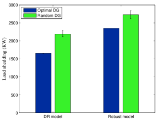
Figure 4: Comparisons of optimal and random DG allocation in the 33-node distribution system

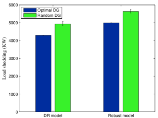
Figure 5: Comparisons of optimal and random DG allocation in the 69-node distribution system

IV-B On the value of optimal DG allocation

We conduct a set of experiments to evaluate the value of optimally allocating DG units in the distribution system. In Fig. 4 and Fig. 5 we compare the level of load shedding when DG units are optimally located with the case when DG units are randomly deployed. For “optimal DG”, we solve the DR and RO models. For “random DG”, we first randomly place DGs and then solve both models to configure the distribution system. We perform the experiments for 5 times and report the average values to mitigate the randomness. From Figs. 4 and 5, we observe that locating DGs properly can significantly decrease the load shedding. This is because when the distribution system is affected by contingencies, the loads in islanded zones can be effectively picked up by the existing DG resources. As a result, better DG allocation significantly enhances the system resiliency.

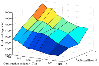
Figure 6: Average load shedding under various line construction budget and affected lines for the 33-node distribution system

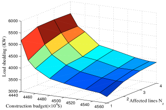
Figure 7: Average load shedding under various line construction budget and affected lines for the 69-node distribution system

IV-C Impact of construction and contingency budgets

In Figs. 6 and 7, we depict the amounts of expected load shedding under various line construction budgets (i.e., $B_{y}$) and contingency budgets (i.e., $N_{z}$). From these two figures, we observe that load shedding reduces as $B_{y}$ increases and as $N_{z}$ decreases, i.e., as we allow the contingency to affect less power lines in the DR model. This is intuitive. In addition, we observe that load shedding is sensitive to the construction budget. For example, by increasing the budget from $4440$\times 10^{4}$ to $4480$\times 10^{4}$ when $N_{z}=4$ in Fig. 7, the load shedding decreases from 5485KW to 4297KW, which means that a 0.9% budgetary rise translates into a 21.6% load shedding reduction. Furthermore, we observe that the impact of construction budget is marginally diminishing. For example, increasing the budget from $4500$\times 10^{4}$ to $4560$\times 10^{4}$ (i.e., by 1.3%) results in a 6.7% load shedding reduction. This observation highlights the necessity of implementing a cost-effective distribution configuration planning.

IV-D Worst-case contingency distribution

The worst-case contingency distribution for the 69-node distribution system is reported in Table II. We select a subset of representative scenarios to display and omit other scenarios with smaller probability values. From this table, we observe that the contingency probabilities for different power lines are highly heterogeneous. This provides the system operator a guideline on the system vulnerability and a meaningful contingency probability distribution that can be used in other vulnerability analyses.

TABLE II: Worst-case contingency distribution for the 69-node system

Scenario	Affected lines	Probability
1	6-15,13-14,34-35,39-40	0.0031
2	5-26,6-15,12-13,38-39	0.0025
3	1-2,5-26,38-39,39-40	0.0021
4	12-13,13-14,38-39,61-62	0.0002

Proof:

We rewrite $\max_{\mathbb{P}\in\mathbb{D}}E_{\mathbb{P}}[Q(\mathbf{g},{\mathbf{z}})]$ as:

$$\max_{\mathbb{P}\in\mathbb{D}}E_{\mathbb{P}}[Q(\mathbf{g},{\mathbf{z}})]=\max_{\mathbb{P}}\int_{\mathfrak{D{(\mathbf{g})}}}{Q(\mathbf{g},\mathbf{z})d{\mathbb{P}}},$$ (12a)

s.t. $$\int_{\mathfrak{D{(\mathbf{g})}}}{d{\mathbb{P}}}=1,$$ (12c)

$$\int_{\mathfrak{D{(\mathbf{g})}}}{(1-z_{mn,t})d{\mathbb{P}}}\leq\mu_{mn,t}^{max},\forall{(m,n)\in\mathcal{E}},\ \forall{t\in\mathcal{T}}.$$

The feasible region of the problem (12a)–(12c) has an interior point. In other words, there exists a $\hat{\mathbb{P}}$ that satisfies constraint (12c) at equality and constraint (12c) strictly. For example, we can set $\hat{\mathbb{P}}$ to be the probability distribution solely supported on the scenario that no contingency arises in the system, i.e., $z_{mn,t}=1,\forall{(m,n)\in\mathcal{E},t\in\mathcal{T}}$. Thus, the Slater’s condition holds between the problem (12a)–(12c) and the following dual formulation:

$$\min_{\mathbf{\boldsymbol{\beta}}\geq 0,\gamma}\gamma+\sum_{t\in\mathcal{T}}\sum_{(m,n)\in\mathcal{E}}\mu_{mn,t}^{max}\beta_{mn,t},$$ (13)

s.t.

$$\gamma+\sum_{t\in\mathcal{T}}\sum_{(m,n)\in\mathcal{E}}(1-z_{mn,t})\beta_{mn,t}\geq Q(\mathbf{g},\mathbf{z}),\ \forall{\mathbf{z}\in\mathfrak{D{(\mathbf{g})}}}.$$ (14)

where $\gamma$ and $\mathbf{\boldsymbol{\beta}}$ are dual variables associated with constraints (12c) and (12c), respectively. In the dual formulation, we observe that the optimal $\gamma$ should satisfy

$$\gamma=\max_{\mathbf{z}\in\mathfrak{D{(\mathbf{g})}}}\bigg{\{}Q(\mathbf{g},\mathbf{z})-\sum_{t\in\mathcal{T}}\sum_{(m,n)\in\mathcal{E}}(1-z_{mn,t})\beta_{mn,t}\bigg{\}}.$$ (15)

Substituting $\gamma$ from (15) to the objective function (13) completes the proof. ∎

Proof:

With variables $g$ and $u^{j}$ fixed at $\hat{g}^{R}$ and $\hat{u}^{j}$, respectively, we take the dual of formulation (9a)–(9c) to obtain:

$$\max_{\psi\geq 0}\ \ \sum_{j=1}^{R}\psi_{j}\Bigl{(}\sum_{t\in\mathcal{T}}\sum_{n\in\mathcal{N}}s^{j}_{nt}\Bigr{)}$$ (16a)

s.t. $$\ \sum_{j=1}^{R}\psi_{j}(1-z^{j}_{mn,t})\leq\mu^{max}_{mn,t},$$

$$\ \forall t\in\mathcal{T},\ \ \forall(m,n)\in\mathcal{E},$$ (16b)

$$\ \sum_{j=1}^{R}\psi_{j}=1.$$ (16c)

By constraints (16b)–(16c), $\{\psi_{j}\}_{j=1,\ldots,R}$ characterize a probability distribution supported on scenarios $\{\mathbf{z}^{j}\}_{j=1,\ldots,R}$ such that $\mathbb{P}\{\mathbf{z}=\mathbf{z}^{j}\}=\psi_{j}$, $\forall j=1,\ldots,R$. As the CCG framework terminates at the $R^{\mbox{\tiny th}}$ iteration and by the strong duality of linear programming, formulation (16a)–(16c) is equivalent to the worst-case expectation formulation (6), i.e., these two formulations yield the same optimal value. It follows that $\{\psi_{j}\}_{j=1,\ldots,R}$ characterize the worst-case contingency probability distribution. ∎

References

- [1] A. M. Salman, Y. Li, and M. G. Stewart, “Evaluating system reliability and targeted hardening strategies of power distribution systems subjected to hurricanes,” Reliability Engineering & System Safety, vol. 144, pp. 319–333, 2015.
- [2] L. Che, M. Khodayar, and M. Shahidehpour, “Only connect: Microgrids for distribution system restoration,” IEEE Power and Energy Magazine, vol. 12, no. 1, pp. 70–81, 2014.
- [3] E. O. of the President, “Economic benefits of increasing electric grid resilience to weather outages-august 2013.”
- [4] D. T. Ton and W. P. Wang, “A more resilient grid: The U.S. Department of Energy joins with stakeholders in an R&D plan,” IEEE Power and Energy Magazine, vol. 13, no. 3, pp. 26–34, 2015.
- [5] “President’s Council of Economic Advisers and the U.S. Department of Energy, Economic Benefits of Increasing Electric Grid Resilience to Weather Outages,” Tech. Rep., 2013.
- [6] J. Moreira, E. Miguez, C. Vilacha, and A. F. Otero, “Large-scale network layout optimization for radial distribution networks by parallel computing,” IEEE transactions on power delivery, vol. 26, no. 3, pp. 1946–1951, 2011.
- [7] D. Kumar and S. Samantaray, “Design of an advanced electric power distribution systems using seeker optimization algorithm,” International Journal of Electrical Power & Energy Systems, vol. 63, pp. 196–217, 2014.
- [8] Z. Wang and J. Wang, “Self-healing resilient distribution systems based on sectionalization into microgrids,” IEEE Transactions on Power Systems, vol. 30, no. 6, pp. 3139–3149, 2015.
- [9] S. A. Arefifar, Y. A.-R. I. Mohamed, and T. H. EL-Fouly, “Comprehensive operational planning framework for self-healing control actions in smart distribution grids,” IEEE Transactions on Power Systems, vol. 28, no. 4, pp. 4192–4200, 2013.
- [10] W. Yuan, J. Wang, F. Qiu, C. Chen, C. Kang, and B. Zeng, “Robust optimization-based resilient distribution network planning against natural disasters,” IEEE Transactions on Smart Grid, vol. 7, no. 6, pp. 2817–2826, 2016.
- [11] S. Ma, B. Chen, and Z. Wang, “Resilience enhancement strategy for distribution systems under extreme weather events,” IEEE Transactions on Smart Grid, vol. 9, no. 2, pp. 1442–1451, 2016.
- [12] A. Samui, S. Singh, T. Ghose, and S. Samantaray, “A direct approach to optimal feeder routing for radial distribution system,” IEEE Transactions on Power Delivery, vol. 27, no. 1, pp. 253–260, 2012.
- [13] A. Navarro and H. Rudnick, “Large-scale distribution planning–part I: Simultaneous network and transformer optimization,” IEEE Transactions on Power Systems, vol. 24, no. 2, pp. 744–751, 2009.
- [14] K. Mahmoud, N. Yorino, and A. Ahmed, “Optimal distributed generation allocation in distribution systems for loss minimization,” IEEE Transactions on Power Systems, vol. 31, no. 2, pp. 960–969, 2016.
- [15] B. R. Pereira, G. R. M. da Costa, J. Contreras, and J. R. S. Mantovani, “Optimal distributed generation and reactive power allocation in electrical distribution systems,” IEEE Transactions on Sustainable Energy, vol. 7, no. 3, pp. 975–984, 2016.
- [16] Y. Atwa, E. El-Saadany, M. Salama, and R. Seethapathy, “Optimal renewable resources mix for distribution system energy loss minimization,” IEEE Transactions on Power Systems, vol. 25, no. 1, pp. 360–370, 2010.
- [17] Z. Liu, F. Wen, and G. Ledwich, “Optimal siting and sizing of distributed generators in distribution systems considering uncertainties,” IEEE Transactions on power delivery, vol. 26, no. 4, pp. 2541–2551, 2011.
- [18] E. Míguez, J. Cidrás, E. Díaz-Dorado, and J. L. García-Dornelas, “An improved branch-exchange algorithm for large-scale distribution network planning,” IEEE Transactions on Power Systems, vol. 17, no. 4, pp. 931–936, 2002.
- [19] A. Y. Abdelaziz, F. Mohamed, S. Mekhamer, and M. Badr, “Distribution system reconfiguration using a modified tabu search algorithm,” Electric Power Systems Research, vol. 80, no. 8, pp. 943–953, 2010.
- [20] M. Lavorato, J. F. Franco, M. J. Rider, and R. Romero, “Imposing radiality constraints in distribution system optimization problems,” IEEE Transactions on Power Systems, vol. 27, no. 1, pp. 172–180, 2012.
- [21] S. A. El Batawy and W. G. Morsi, “Optimal secondary distribution system design considering rooftop solar photovoltaics,” IEEE Transactions on Sustainable Energy, vol. 7, no. 4, pp. 1662–1671, 2016.
- [22] J. Li, X.-Y. Ma, C.-C. Liu, and K. P. Schneider, “Distribution system restoration with microgrids using spanning tree search,” IEEE Transactions on Power Systems, vol. 29, no. 6, pp. 3021–3029, 2014.
- [23] E. Delage and Y. Ye, “Distributionally robust optimization under moment uncertainty with application to data-driven problems,” Operations research, vol. 58, no. 3, pp. 595–612, 2010.
- [24] P. Xiong, P. Jirutitijaroen, and C. Singh, “A distributionally robust optimization model for unit commitment considering uncertain wind power generation,” IEEE Transactions on Power Systems, vol. 32, no. 1, pp. 39–49, 2017.
- [25] Q. Bian, H. Xin, Z. Wang, D. Gan, and K. P. Wong, “Distributionally robust solution to the reserve scheduling problem with partial information of wind power,” IEEE Transactions on Power Systems, vol. 30, no. 5, pp. 2822–2823, 2015.
- [26] F. Qiu and J. Wang, “Distributionally robust congestion management with dynamic line ratings,” IEEE Transactions on Power Systems, vol. 30, no. 4, pp. 2198–2199, 2015.
- [27] A. Bagheri, J. Wang, and C. Zhao, “Data-driven stochastic transmission expansion planning,” IEEE Transactions on Power Systems, vol. 32, no. 5, pp. 3461–3470, 2017.
- [28] T. L. Magnanti and L. A. Wolsey, “Optimal trees,” Handbooks in operations research and management science, vol. 7, pp. 503–615, 1995.
- [29] M. E. Baran and F. F. Wu, “Network reconfiguration in distribution systems for loss reduction and load balancing,” IEEE Transactions on Power delivery, vol. 4, no. 2, pp. 1401–1407, 1989.
- [30] H. Gao, Y. Chen, S. Mei, S. Huang, and Y. Xu, “Resilience-oriented pre-hurricane resource allocation in distribution systems considering electric buses,” Proceedings of the IEEE, 2017.
- [31] A. Arab, A. Khodaei, S. K. Khator, K. Ding, V. A. Emesih, and Z. Han, “Stochastic pre-hurricane restoration planning for electric power systems infrastructure,” IEEE Transactions on Smart Grid, vol. 6, no. 2, pp. 1046–1054, 2015.
- [32] E. Yamangil, R. Bent, and S. Backhaus, “Designing resilient electrical distribution grids,” arXiv preprint arXiv:1409.4477, 2014.
- [33] Y. Sa, “Reliability analysis of electric distribution lines,” Ph.D. dissertation, McGill University, 2002.
- [34] C. Zhao and R. Jiang, “Distributionally robust contingency-constrained unit commitment,” IEEE Transactions on Power Systems, vol. 33, no. 1, pp. 94–102, 2018.
- [35] B. Zeng and L. Zhao, “Solving two-stage robust optimization problems using a column-and-constraint generation method,” Operations Research Letters, vol. 41, no. 5, pp. 457–461, 2013.
- [36] G. P. McCormick, “Computability of global solutions to factorable nonconvex programs: Part I–convex underestimating problems,” Mathematical programming, vol. 10, no. 1, pp. 147–175, 1976.