aiAIArtificial Intelligence \newabbreviationnlpNLPNatural Language Processing \newabbreviationSeq2SeqSeq2Seqsequence-to-sequence \newabbreviationvaeVAEVariational Autoencoders \newabbreviationdaeDAEDeterministic Autoencoders \newabbreviationvedVEDVariational Encoder-Decoder \newabbreviationdedDEDDeterministic Encoder-Decoder \newabbreviationklKLKullback-Leibler \newabbreviationmlMLMachine Learning \newabbreviationannANNArtificial Neural Networks \newabbreviationcnnCNNConvolutional Neural Network \newabbreviationrnnRNNRecurrent Neural Network \newabbreviationlstmLSTMLong Short Term Memory \newabbreviationreluReLURectified Linear Unit \newabbreviationgruGRUGated Recurrent Unit \newabbreviationelboELBOEvidence Lower Bound \newabbreviationsgdSGDstochastic gradient descent
Natural Language Generation with Neural Variational Models
by
Hareesh Bahuleyan
A thesis
presented to the University of Waterloo
in fulfillment of the
thesis requirement for the degree of
Master of Applied Science
in
Management Science
Waterloo, Ontario, Canada, 2018
© Hareesh Bahuleyan 2018
Author Declaration
This thesis consists of material all of which I authored or co-authored: see Statement of Contributions included in the thesis. This is a true copy of the thesis, including any required final revisions, as accepted by my examiners.
I understand that my thesis may be made electronically available to the public.
Statement of Contributions
Chapters 4, 5 and 6 of this thesis are based on the following papers:
-
1.
Hareesh Bahuleyan*, Lili Mou*, Olga Vechtomova, and Pascal Poupart. Variational Attention for Sequence-to-Sequence Models. In 27th International Conference on Computational Linguistics (COLING), 2018.
-
2.
Hareesh Bahuleyan, Lili Mou, Kartik Vamaraju, Hao Zhou, and Olga Vechtomova. Probabilistic Natural Language Generation with Wasserstein Autoencoders. arXiv preprint arXiv:1806.08462, 2018
I have contributed to implementation, experimentation, and preparation of the manuscript of the above mentioned papers.
Abstract
Automatic generation of text is an important topic in natural language processing with applications in tasks such as machine translation and text summarization. In this thesis, we explore the use of deep neural networks for generation of natural language. Specifically, we implement two sequence-to-sequence neural variational models - variational autoencoders (VAE) and variational encoder-decoders (VED).
VAEs for text generation are difficult to train due to issues associated with the Kullback-Leibler (KL) divergence term of the loss function vanishing to zero. We successfully train VAEs by implementing optimization heuristics such as KL weight annealing and word dropout. In addition, this work also proposes new and improved annealing schedules that facilitates the learning of a meaningful latent space. We also demonstrate the effectiveness of this continuous latent space through experiments such as random sampling, linear interpolation and sampling from the neighborhood of the input. We argue that if VAEs are not designed appropriately, it may lead to bypassing connections which results in the latent space being ignored during training. We show experimentally with the example of decoder hidden state initialization that such bypassing connections degrade the VAE into a deterministic model, thereby reducing the diversity of generated sentences.
We discover that the traditional attention mechanism used in sequence-to-sequence VED models serves as a bypassing connection, thereby deteriorating the model’s latent space. In order to circumvent this issue, we propose the variational attention mechanism where the attention context vector is modeled as a random variable that can be sampled from a distribution. We show empirically using automatic evaluation metrics, namely entropy and distinct measures, that our variational attention model generates more diverse output sentences than the deterministic attention model. A qualitative analysis with human evaluation study proves that our model simultaneously produces sentences that are of high quality and equally fluent as the ones generated by the deterministic attention counterpart.
Acknowledgements
This thesis would not have been possible without the constant support that I received from a number of people.
First and foremost, I take this opportunity to express my heartfelt gratitude to my supervisor Professor Olga Vechtomova for her guidance throughout this research. I am thankful to her for believing in me and being patient with me since the start of my program. The flexibility that she provided in research has allowed me to learn new topics and explore new ideas. I am deeply indebted to her for having taken the time and effort for reading, reviewing and providing valuable inputs for the reports that I had made.
I am grateful to Dr. Lili Mou for being a mentor, sharing knowledge and providing valuable technical advice. His subject expertise and guidance has played a crucial role in structuring this project. Interactions with him have helped me develop my skills in this field and motivated me to deal with research challenges.
I would like to acknowledge Professor Pascal Poupart for sharing his ideas and providing valuable suggestions.
I thank Professor Jesse Hoey and Professor Stan Dimitrov for taking the time to review my thesis and provide feedback.
I express my gratitude to Vineet John and Ankit Vadehra for the informative discussions and enlightening me on their respective research topics.
Life in Canada would not have have been such an enjoyable journey without the friends that I made here. I thank all my friends for making my stay here at Waterloo, a memorable one.
I am extremely grateful to my parents and my sister for supporting me and being with me even during the toughest times.
Dedication
I dedicate this thesis to my beloved parents and sister for their unconditional love, support, and care.
Glossary
Nomenclature
List of Symbols
Chapter 1 Introduction
1.1 Background
The term was introduced by Professor John McCarthy in 1956, who defined it as “science and engineering of making intelligent machines”. Although the field of covers a broad range of topics, it is generally perceived as the task of making machines achieve human-level intelligence (mccarthy1989artificial).
Fast-forward a few decades, we have achieved great advancements in the field of . For example, the neural network model developed by he2016deep was able to classify images with an accuracy of , surpassing human-level performance. A new milestone was achieved in the area of speech recognition when the system developed by xiong2017microsoft was able to carry out the task with a record minimum word error rate of . There are numerous other commendable accomplishments made in the last decade such as AI beating the human grandmaster in the game of Go (gibney2016google) and the transformations in the transportation industry with the introduction of self-driving vehicles (bojarski2016end).
This recent success can be attributed to the research developments made in a multitude of fields such as computer science, mathematics, neuroscience, psychology, linguistics and so on. This work focuses on the field of computer science, specifically the areas of machine learning and natural language processing.
Machine learning is a sub-field of artificial intelligence in which computers are taught to acquire knowledge or learn from data, without being explicitly programmed. In the past, machine learning algorithms have been used to recognize patterns in the data and make informed decisions. End-to-end automation with machine learning has helped improve the efficiencies of processes and workflows in sectors such as manufacturing. The explosion in the recent years is primarily due to the success of a sub-class of machine learning models known as deep neural networks. This field, known as deep learning, along with the availability of massive amounts of data and powerful hardware for computation has made possible the latest advancements in .
The focus of this work lies in the development and application of deep learning models to . The study of is concerned with how computers can effectively interact with humans using natural language. Broadly speaking, it deals with manipulation, understanding, interpretation and generation of textual and speech data. A few examples of tasks include question answering, sentiment analysis, named-entity recognition and machine translation.
Natural language generation is an task that deals with generation of text in human language. This is challenging because the text generated by a good system has to be syntactically (follow the rules of the language) and semantically (meaningful) correct. In this work, models for natural language generation are explored. In models (sutskever2014sequence), a sequence (of words) is given as input in order to generate another sequence as output. This has applications in tasks such as machine translation where a sentence in English can be fed to the model which generates its corresponding translated sentence in French. Another application is text summarization, where we may attempt to generate a shorter version of a larger body of text, such as a paragraph.
The aim of this work is to integrate attention mechanism into the framework. Attention mechanism has been shown to be particularly useful in improving the performance of sequence-to-sequence tasks such as machine translation (bahdanau2014neural; luong2015effective) and dialog generation (yao2016attentional; mei2017coherent). A class of models that combine deep learning and variational inference, namely (kingma2013auto) have been successfully applied to the task of text generation (bowman2015generating). Attention mechanism enables the model to generate fluent sentences, relevant to the input. Simultaneously, we would be able to generate diverse outputs (for the given input) by sampling from a latent space. This way, the proposed model combines the strengths of the attention mechanism and variational models.
1.2 Motivation and Problem Definition
In this research, we work with deep neural network models known as sequence-to-sequence (Seq2Seq) models that take a sentence as input and generate another sentence as output. Let be the input sequence of words and be the output sequence generated by the model, where and correspond to the number of tokens (words) in the input and output sequences respectively.
Consider a conversational system such as a chatbot, where is the line input by the user and is the line generated by the machine. neural network models can be designed to function as such conversational agents. Traditional conversational systems tend to output safe and commonplace responses such as “I don’t know” (li2015diversity). This is because the line “I don’t know” tends to appear in the training dataset with a high frequency. One cannot label such a generic response as incorrect, since it tends to be a valid response (refer Table 1.1). However, such responses make the conversational agent uninteresting and less engaging.
| Input: What are you doing? | |
|---|---|
| I don’t know. | Get out of here. |
| I don’t know! | I’m going home. |
| Nothing. | Oh, my god! |
| Get out of the way. | I’m talking to you. |
| Input: What is your name? | |
| I don’t know. | My name is Robert. |
| I don’t know! | My name is John. |
| I don’t know, sir. | My name’s John. |
| Oh, my god! | My name is Alice. |
| Input: How old are you? | |
| I don’t know. | Twenty-five. |
| I’m fine. | Five. |
| I’m all right. | Eight. |
| I’m not sure. | Ten years old. |
The motivation for this work is derived from the above example. We would like to be able to generate a diverse set of responses () for a given input line (). Neural variational models can be used to encode input data into latent variables. It is further possible to sample multiple points from the latent space in order to generate diverse outputs. Attention mechanisms such as those proposed in (bahdanau2014neural; luong2015effective) have significantly improved the performance of sequence-to-sequence text generation tasks. Attention mechanisms help in dynamically aligning the source and target during generation.
In variational Seq2Seq, however, the attention mechanism unfortunately serves as a “bypassing” mechanism. In other words, the variational latent space does not need to learn much, as long as the attention mechanism itself is powerful enough to capture source information.
In this work, we study how attention mechanisms can be integrated into variational neural models, while avoiding the issue of “bypassing”. In this work, we propose a variational attention mechanism to address this problem. This is done by modeling the attention context vector as random variables by imposing a probabilistic distribution. By doing this we would be able to combine the stochasticity introduced by variational models with the alignment capabilities achieved through attention mechanism.
1.3 Contributions
The contributions of this thesis are multi-fold and listed below:
-
1.
A variational auto-encoder (VAE) is first designed following the work of bowman2015generating. We overcome the difficulties associated with training VAE models for natural language generation by employing strategies such as (1) annealing coefficient of the loss term and (2) word-dropout. We also propose new and improved annealing schedules. The effectiveness of the model is demonstrated by random sampling and linear interpolation of sentences in the latent space.
-
2.
We discover a “bypassing” phenomenon in VAEs that causes the latent or variational space to be ignored during training. This results in the model becoming more deterministic in nature; the evidence for which is revealed through the lower diversity of generated sentences.
-
3.
We realize that traditional attention mechanism in variational encoder-decoder (VED) models serves as a “bypassing” connection. To this end and in contrast to previous models that utilize attention in a deterministic manner, we propose a variational attention mechanism that can be applied in the context of VED models. In the proposed framework, the attention context vector is modeled as a random variable that can be sampled from a distribution.
-
4.
We propose two plausible priors for modeling the prior distribution of the attention context vector in the variational attention VED framework. Both the priors work equally well in alleviating the problem of “bypassing”, which is observed in the VED baselines with deterministic attention.
-
5.
Experiments are carried out on two tasks –– question generation and conversational systems. Quantitative evaluation metrics show that the proposed variational attention yields a higher diversity than variational Seq2Seq with deterministic attention, while retaining high quality of generated sentences. A qualitative analysis with human evaluation study also supports our claim regarding the fluency of sentences generated by the proposed model.
1.4 Chapter Outline
The rest of this thesis report is organized as follows:
-
•
Chapter 2 provides a background and brief overview of the deep learning techniques used in this work, along with related work in the area of models.
-
•
Chapter 3 describes neural network architecture in depth.
-
•
Chapter 4 introduces variational inference and a detailed description of variational autoencoders. The heuristics involved in training VAEs for natural language generation are presented followed by the results.
-
•
Chapter 5 outlines the bypassing phenomenon that we discover, if the VAE architecture is not designed properly and its implications.
-
•
Chapter 6 provides details about the proposed variational attention model, which is compared to the traditional deterministic attention. We demonstrate the benefits of our model through qualitative and quantitative evalutation.
-
•
Chapter 7 gives a summary of the work, followed by conclusions and scope for future work.
Chapter 2 Background and Related Work
In this chapter, different classes of machine learning models are first outlined. Then, we introduce deep learning and the structure of artificial neural networks. Following this, we describe recurrent neural networks, specifically long short term memory networks, which are widely used in the NLP literature. Since this work deals with text generation, we review the recent advances in this area, specifically sequence-to sequence models, attention mechanism and audoencoding. The chapter concludes with the related work in the tasks of question generation and dialog systems, which are the two experiments conducted in this study, to evaluate the proposed model.
2.1 Machine Learning
The science of involves enabling computers to learn from data, without being explicitly programmed. Data is used to train the system to perform a specific task. The model, which uses some form of mathematical optimization and statistical methods, recognizes the patterns and intricacies within the data. This can be then used to automate tasks or guide decision making, simply based on data and the mathematical model.
Machine learning is being increasingly used in our day-to-day lives. For example, all email service providers today use to filter out spam emails. Similarly, the online shopping recommendations provided to us by ecommerce websites is based on . The field of machine learning is developing at a fast pace. Researchers have been developing algorithms and new methodologies and also simultaneously applying these techniques to new application areas (such as medical diagnosis (kourou2015machine; foster2014machine) and climate change (lakshmanan2015machine)). The evolution of intelligent systems are definitely beneficial because it makes processes more efficient, and at the same time, requiring minimal human intervention.
Broadly speaking, machine learning methodologies can be classified into two categories: supervised learning and unsupervised learning. At a high level, this categorization is based on how the learning process is carried out. The following subsections describe each one with examples.
2.1.1 Supervised Learning
In supervised machine learning, we provide the model with sample inputs and their corresponding ground truth labels. Here, the task of the machine learning algorithm is usually to modify the model parameters, such that it obtains the desired output for the given input. The important point to note here is that we have labelled outputs corresponding to each input used to train the model. After sufficient training, if the model is provided with a new unseen input data point, it should be able to predict the target, based on what it has previously learnt.
To understand supervised learning with the help of an example consider the task of image classification. We feed the machine learning model with images of huskies, retrievers, dachshunds, etc. and label them as dogs. Similarly, we can provide images of pigeons, eagles, sparrows, etc., all labelled as birds. The model tries to learn from the image pixel values and their corresponding class labels, as to what would be the characteristics that differentiate dogs from birds, which is then used to classify new images.
2.1.2 Unsupervised Learning
In contrast to the approach discussed in Section 2.1.1, the data provided to an unsupervised machine learning model will not contain labels or corresponding target values. The task of such models would be to identify patterns of similarity or differences within the input data points. It can also be used for detecting anomalies, wherein some parts of the data may not fit well with the rest of the data.
An example of unsupervised learning task would be clustering of documents by topic. Assume that we provide an unsupervised machine learning model with unlabelled documents pertaining to different topics such as sports, politics and entertainment. A good model should be able to automatically cluster similar documents (belonging to the same topic) together, using information such as the word usage and writing style.
Other areas in machine learning include topics such as semi-supervised learning and reinforcement learning, which are not covered in this text.
2.2 Deep Learning
are an important class of machine learning models, used for both supervised and unsupervised tasks. The structure and functioning of s are loosely inspired by biological neural networks. The brain consists of a large number of interconnected neurons, which s try to mimic. s consist of multiple layers of simple processing units known as nodes, which are connected by edges with weights (gurney2014introduction) (refer to Section 2.2.1 for details).
Over the last decade, there has been an increasing interest in neural network architectures consisting of many layers. Along with the availability of massive amounts of data and powerful hardware for computation, such model architectures were able to outperform humans in a number of cognitive tasks (schmidhuber2015deep; najafabadi2015deep). This led to the creation of a sub-field of machine learning known as deep learning (referring to deep neural networks) (lecun2015deep).
The most basic version of an model is a feed-forward neural network. However, there exist other architectures such as (williams1989learning; elman1990finding) and (lecun1995convolutional). s perform particularly well on sequential data such as in natural language processing (where sentences are considered as sequences of words). Hence, the focus of this work will be on s, which are described in detail in Section 2.2.2
2.2.1 Introduction to Neural Networks
In order to understand the computational model of artificial neural networks, one needs to begin from its building block, known as the perceptron (rosenblatt1958perceptron). Inspired from the brain’s neurons, a perceptron is a simple computational model that takes in one or more inputs and provides a single value as output. This is illustrated in Figure 2.1. Based on this output and a pre-defined threshold, the perceptron acts as a binary classifier, i.e., if the output value is greater than the threshold, the input is assigned to class 1, else it is assigned to class 0.
Let be the inputs to the perceptron model. are the series of model weights corresponding to each input variable. This simple model consists of two operations:
-
•
The first step is to multiply each input with its weight, followed by a summation. To this result, we also add the bias term so that the model has a flexibility for location shift.
-
•
Next, we assign a class label (either 0 or 1), based on a binary activation function which requires a pre-defined threshold (refer Figure 2.1).
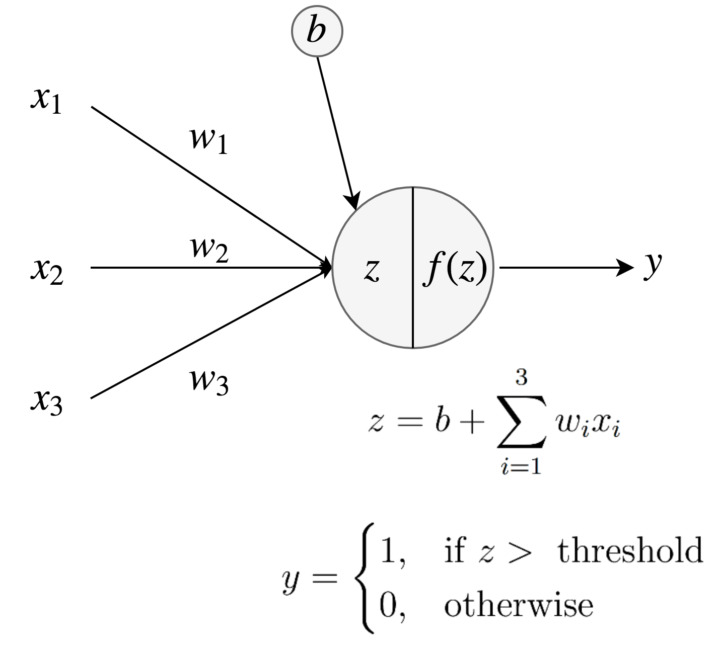
The result is the predicted value of output corresponding to the given set of inputs. In order for the predicted output to be close to the desired output (ground truth), we would need to make adjustments to the weights and bias term .
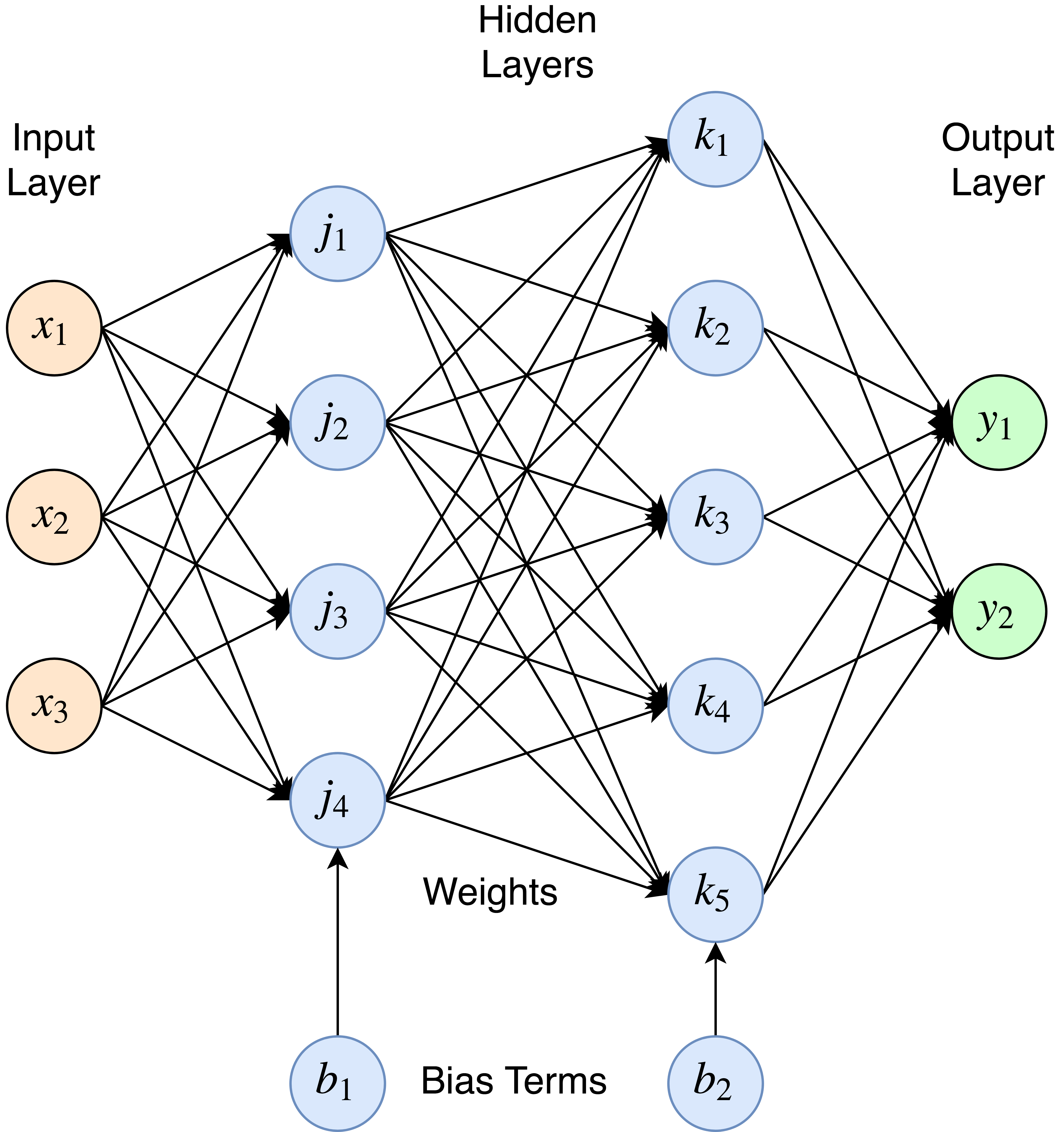
However, modern neural networks do not use the simple perceptron anymore. Instead, they consist of computational units known as neurons (or nodes), which replace the simple binary activation function with non-linear functions such as , or . It is possible to combine multiple layers of neurons to form a more powerful model known as the feed-forward neural network. Each neuron is connected to every other neuron in the previous and next layer. However, there are no connections between neurons within the same layer. As illustrated in Figure 2.2, there can be multiple inputs and multiple outputs which are connected via a number of hidden layers. The input at each neuron gets transformed by weighted summation followed by non-linear activation. The computation happens starting from the input layer, all the way till the output layer and is known as forward propagation. Feed-forward neural network are capable of learning non-linear representations of the data and have been successfully applied to many classification and regression tasks.
Although artificial neural networks have been around since the 1960s, it was not until the late 1980s that an efficient training procedure for s was discovered. There existed no structured methodology to adjust the model weights, other than by trial and error. Researchers like rumelhart1986learning and werbos1990backpropagation contributed to the development of the method known as backpropagation of errors, which made it possible to estimate the weights in an ANN model. Backpropagation makes use of the chain rule of differentiation, and computes the gradients in an iterative manner.
In order to develop an intuition of backpropagation, it is necessary to understand how an optimization method known as Gradient Descent works. In neural networks, we compare the predicted output to the actual output based on a pre-defined loss function. Common examples of loss functions are mean squared error (MSE) and negative log-likelihood (NLL). Our objective is to adjust the model weights in a way that minimizes the loss. It is mathematically guaranteed that moving in the direction of the gradient of the loss function (derivative with respect to the model weights), results in loss minimization.
Assume to be the loss function, with being the model weights. We start with a random initialization of the weights, followed by an iterative update rule as shown in Equation 2.1,
| (2.1) |
where, is a hyperparameter (set by the user) known as the learning rate, which corresponds to the step size towards the local minima in each iteration and refers to the gradient operator. While a low learning rate results in the training process to progress slowly, a high learning rate may cause the training to diverge from the minima. Because of this trade-off, the learning rate needs to be set carefully. We stop the iteration process either when we reach the pre-defined maximum number of iterations (known as epochs) or when the change in model weights between iterations is smaller than a specified threshold . Readers are referred to bishop2006prml for further details on backpropagation and Gradient Descent.
2.2.2 Recurrent Neural Networks
One of shortcomings of feed forward neural networks such as the one illustrated in Figure 2.2 is that it assumes that all input data are independent of each other. As a result, it fails to capture the notion of sequential order which is present in some types of data. Consider the task of predicting the next character in a word. If we are given an incomplete word such as ‘neura’, one can guess that the next character in the sequence would be ‘l’ and the word is ‘neural’. However, if the order of the previous characters was jumbled (such as ‘renau’) and provided independently, it would be very difficult to identify the final character. This is where s are found to be extremely useful. One of the earliest versions of the recurrent neural network was proposed by elman1990finding. The input to an is provided in a sequential manner, and the network makes use of the inputs in the previous timesteps in order to make a decision at the current timestep.
A recurrent neural network can be depicted as a network with loops (see Figure 2.3), through which information is transferred between timesteps of the network. By unrolling the network, we realize that the information at each timestep passes through multiple copies of the same network (olahlstm).
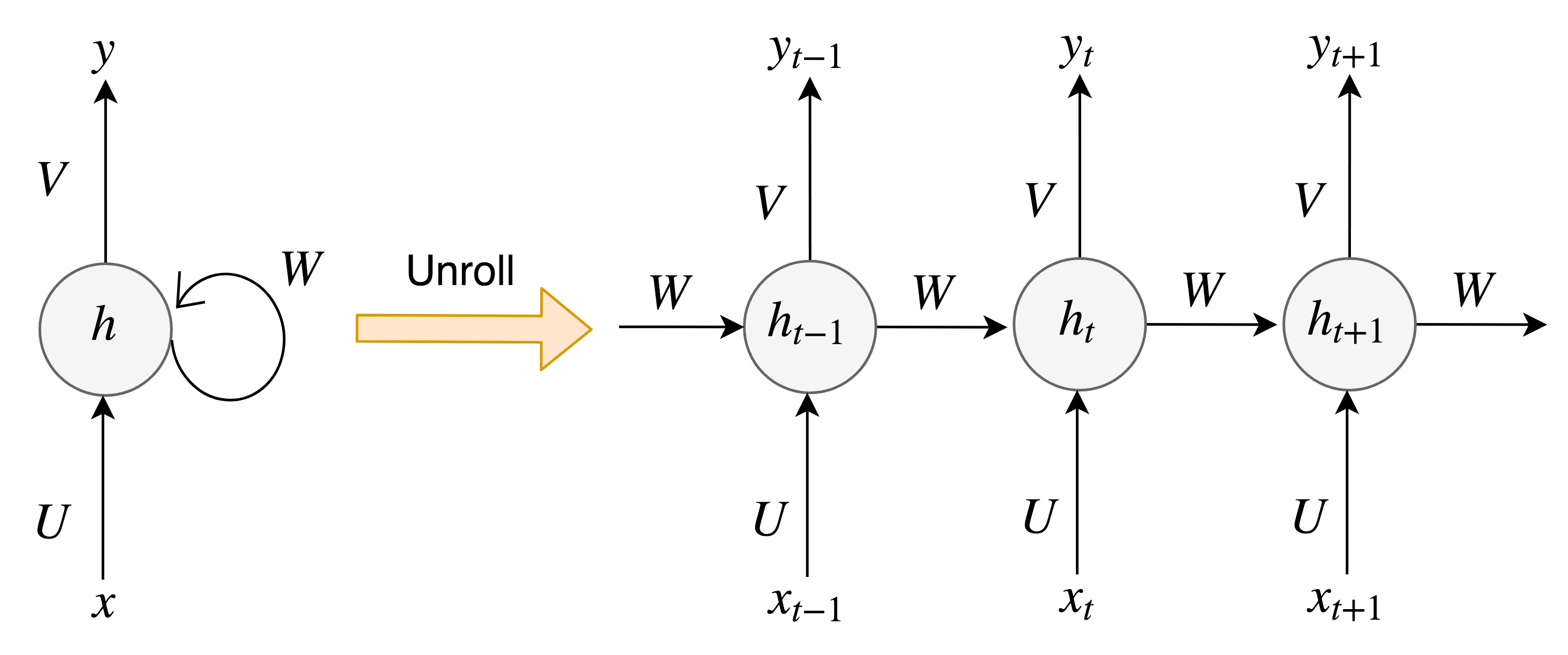
The notation in Figure 2.3, adapted from (britzrnn) is described below:
-
•
corresponds to the input at each timestep
-
•
refers to the output at each timestep
-
•
is called the hidden state at each timestep , and is calculated using the input at the current timestep and the hidden state from the previous timestep , i.e.,
(2.2) where corresponds to some non-linear activation function such as or . In RNN literature, is also referred to as the memory because in theory, it is assumed to capture information from all previous timesteps. However, this does not hold true in practice since the RNN memory fails to remember information beyond few previous timesteps.
-
•
, and are weight matrices. From the unrolled RNN figure, one can note that these weights are shared across all timesteps of the RNN. Doing this reduces the model complexity by reducing the number of parameters that need to be optimized. Moreover, we aim to perform the same operation across timesteps, just with different inputs.
Training of s is done via an extension of the backpropagation algorithm, known as backpropagation through time (BPTT). As discussed earlier, RNNs perform well on sequential data and have been extensively used for tasks such as language modelling (mikolov2010recurrent), text generation (graves2013generating) and speech recognition (graves2013speech).
2.2.3 Long Short Term Memory
In practice, vanilla RNNs suffer from the inability to capture long term dependencies. In other words, when the length of input sequence becomes large, RNNs are unable to remember the dependencies between inputs which are far apart in the sequence. The reason for this is attributed to the vanishing/exploding gradient problem (pascanu2013difficulty). This happens due to numeric underflow or overflow, i.e., when the multiplication of derivative terms during backpropagration become extremely small or very large. Exploding gradients can be an easier problem to solve - by truncating gradients when their absolute value crosses a pre-specified threshold (pascanu2012understanding).
In order to circumvent the issue of vanishing gradients, extensions to the vanilla RNN architecture, Units (hochreiter1997long) and (chung2014empirical) were proposed. This thesis work makes use of RNNs with LSTM units, which will be described in this section.
In s, we replace the simple activation function of Equation 2.2 with an entire module, also known as cell. The input to each repeating module consists of and along with a new term , known as the cell state. The output at timestep now includes both and . This is depicted in Figure 2.4.
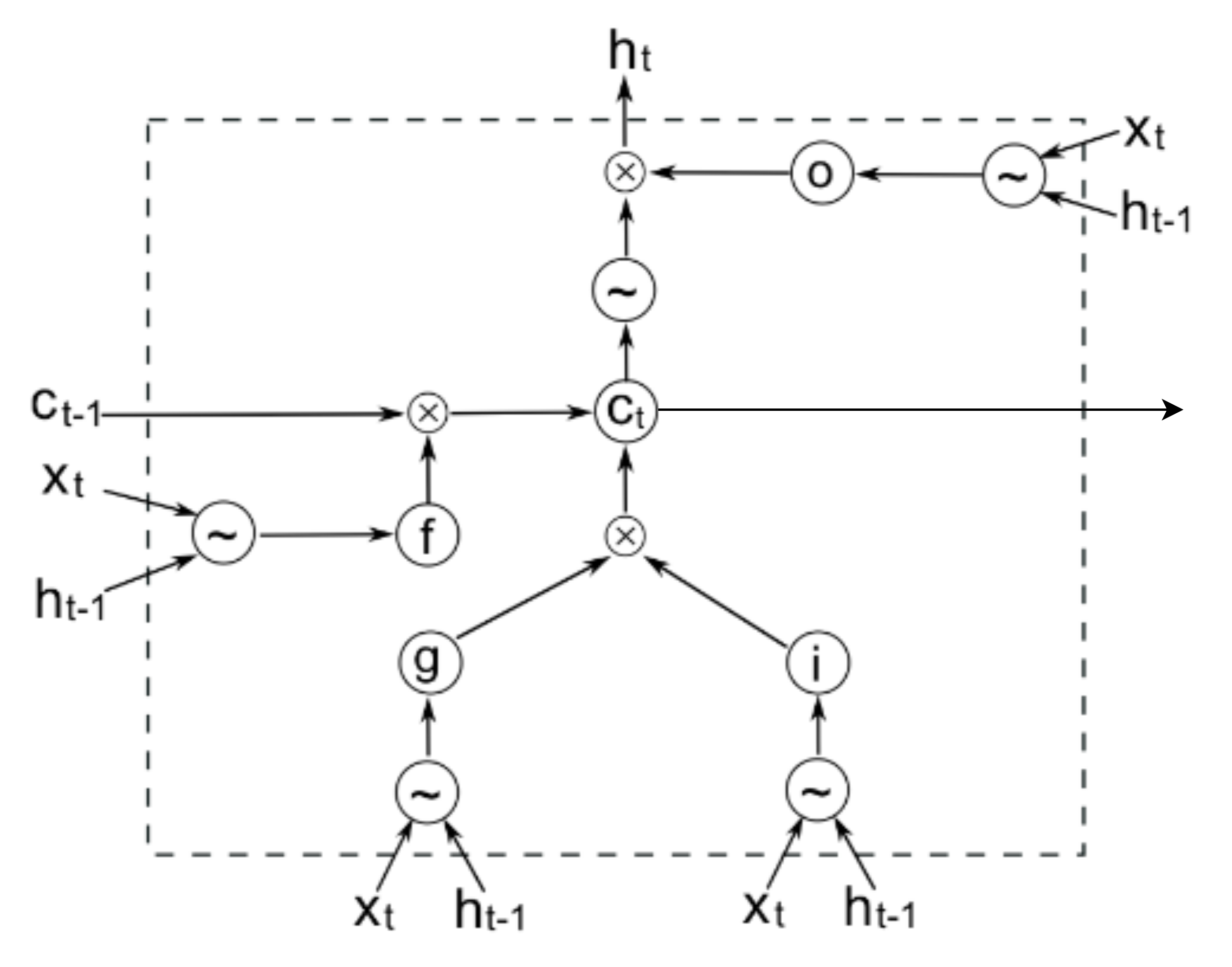
The LSTM unit consists of gated operations and element-wise multiplications. Gates, represented by activations (which output values between 0 and 1) essentially decide how much of the incoming information should flow through. The equations of the three adaptive gates namely, the input gate (), the forget gate () and the output gate () are given below:
| (2.3) | |||
| (2.4) | |||
| (2.5) |
where denotes the function. Each of the gates has its own weights (, and ) and require as input the previous hidden state and the current input . In addition, we also compute a candidate cell state vector () as follows:
| (2.6) |
We now have all the vectors required to determine the cell state () and hidden state () of the current timestep:
| (2.7) | |||
| (2.8) |
where refers to the element-wise multiplication operator.
To summarize the procedure, we start by setting the cell state and hidden state of the initial timestep, namely and as zero vectors. Then, the values of and are computed sequentially for each timestep using Equations 2.3 to 2.8, till the end of the sequence is reached.
s excel at capturing long term dependencies and have been applied to a number of tasks: sequence tagging (huang2015bidirectional), relationship classification (xu2015classifying), textual entailment (rocktaschel2015reasoning), machine comprehension (cheng2016long), sentiment analysis (tai2015improved) and many more.
Bi-directional LSTMs
LSTMs work based on the principle that the output at the current timestep is dependent on the inputs (and outputs) at previous timesteps. However, in some tasks such as part-of-speech (POS) tagging (huang2015bidirectional) and text-to-speech (TTS) synthesis (fan2014tts), it is useful to be aware of the elements in the future timesteps. Bidirectional LSTMs are known to perform better than regular LSTMs in such scenarios (schuster1997bidirectional). Essentially, a bidirectional LSTM consists of two LSTMs stacked one on top of the other - the first LSTM reads the sequence in the forward manner (e.g., a regular sentence), while the sequence is fed in the backward direction to the second LSTM (e.g., the same sentence with its word order reversed). The output vectors of the two LSTMs are then concatenated and fed to the next layer in the neural network.
2.2.4 Sequence-to-Sequence Models
In natural language processing, sequence-to-sequence tasks usually refer to the ones in which the model takes as input one sequence and generates another sequence as output (instead of a single value). The sequence can range from whole documents to individual words. In the case of documents or sentences, the individual tokens that form the sequence are words. In contrast, when words themselves are treated as sequences, their characters become the individual tokens.
models are typically implemented with the help of two recurrent neural networks (usually an or ). In the most basic version, the input/source sequence is fed token-by-token to the first (encoder), which computes a vector representation for the whole sequence. This vector representation becomes the starting point for the second (decoder), which generates the output/target sequence, again in a token-by-token manner.
sutskever2014sequence first introduced models for the task of machine translation. Their LSTM based approach was able to achieve a translation performance close to the state-of-the-art. The advantage of their method is that it could be trained completely end to end (assuming the availability of a parallel corpora), without the need for any manual feature engineering. In order to generate vector representations for sentences, similar to the idea of word2vec (mikolov2013distributed) for words, kiros2015skip proposed a learning approach. Essentially the network would be trained to generate a given sentence, based on two of its neighbouring sentences (previous and next).
In NLP, Seq2Seq models are extensively used for the text generation. yin2015neural developed a Seq2Seq model trained on question-answer pairs and knowledge-base triples for the task of answering short factoid questions. Seq2Seq models have opened up the possibility to train dialog sytems in an end-to-end manner, without the need for any hand-crafted features (vinyals2015neural). Modifications to the original negative log likelihood objective function (li2015diversity) and beam search optimization (wiseman2016sequence) have made dialog systems to be more human-like.
models have also been successfully applied to multimodal data. For instance, venugopalan2015sequence demonstrate how LSTMs could be used to generate textual descriptions when they are trained with video clips as input. In (yao2015sequence), the authors develop a model to synthesize speech from textual data.
Since generation of text is the focus of this thesis work, LSTM based sequence-to-sequence models are used following previous research in this area.
2.2.5 Auto-encoding
Autoencoding is an unsupervised learning technique in which we provide an input (such as image or text) to a model, learn an intermediate representation and then try to reconstruct the original input from this representation. The model is usually an artificial neural network, and the intermediate representation typically has lower dimensionality than the original input (hinton2006reducing). Hence, the goal becomes to learn an efficient encoding that stores just the necessary information required for reconstruction.
The intermediate representation can later be used for other supervised tasks in the machine learning pipeline. For example, consider the task of recognizing hand written digits. We train an autoencoder with images of digits from 0 to 9. Next, instead of using the original image, we could use their intermediate representations to train a feed forward neural network to classify these digits. Autoencoders have been successfully applied to solve problems such as image super-resolution (zeng2017coupled) and speech enhancement (lu2013speech). Since the lower dimension representations generated by autoencoders are useful in identifying patterns pertaining to the original data, they have also been applied to anomaly detection (malhotra2016lstm).
In the domain of , autoencoders are usually models. s encode the input sentence into its latent representation. The decoder then uses this representation to reconstruct and generate the original sentence. In (andrew2015semi), the authors demonstrate how a sequence autoencoder can serve as a ‘pretraining’ method for enhancing the performance of downstream supervised tasks. Autoencoders can be used not just to represent sentences, but also paragraphs and documents (li2015hierarchical).
2.2.6 Attention Mechanism
Broadly speaking, attention mechanism in neural networks is a way to guide the training process, by informing the model as to what parts of inputs or features it needs to focus on, in order to accomplish the task at hand. In this section, we will review the attention mechanisms used in NLP. This is different from visual attention in computer vision tasks such as image captioning (xu2015show) and object detection (borji2014look).
The two popular attention mechanisms used in models are Luong Attention (luong2015effective) and Bahdanau Attention (bahdanau2014neural). Both of these models were introduced for machine translation, where they were shown to perform better than vanilla Seq2Seq models. Attention mechanisms achieve this by aligning tokens on the target side to the tokens on the source side. While the core idea behind both attention mechanisms remain the same, the method in which the attention context vector is computed is different - it takes a multiplicative form in Luong Attention whereas in Bahdanau Attention it has an additive form.
To explain this Seq2Seq attention mechansim intuitively, consider the task of translating the following sentence from French to English: c’est un chien that is a dog. During the decoding phase, when we arrive at the timestep that decodes the word dog, the model looks at each word on the source side and has to identify that the word chien, is where it has to focus on, thereby giving that particular source token the highest weight when computing the attention context vector. The mathematical details pertaining to how attention mechanism works will be detailed in Chapter 6.
Apart from machine translation, attention mechanism has been found to improve the performance of text summarization (rush2015neural), dialog generation (li2017adversarial), textual entailment (rocktaschel2015reasoning), question generation du2017learning and so on.
2.2.7 Variational Inference
In variational inference, we use machine learning and optimization to approximate probability distributions which are otherwise difficult to estimate (blei2017variational). In Bayesian Inference, it is often of interest to compute posterior distributions. This usually involves solving for intractable integrals which becomes cumbersome. In general terms, we try to find an approximate distribution from a family of distributions that is similar to the posterior which we wish to estimate. In other words, we minimize the Kullback-Leibler divergence between the two distributions.
Although there are methods such as mean field approximation (VI) for variational inference, we will focus on variational auto-encoders (VAE) in this work. In comparison to such traditional methods, s leverage modern neural networks which are universal function approximators and are a more powerful density estimator. VAEs were first introduced by kingma2013auto in the image domain, to learn latent representations for images of handwritten digits. What makes VAEs powerful is that these learnt latent representation (approximately) belong to a pre-defined distribution, such as Gaussian with a known mean and variance. This makes it possible to simply sample a vector from this known distribution and to generate the desired image. It is also possible to manipulate the latent representation to change certain characteristics of the input image. For instance, deep2015tejas showed that VAEs could be used as a 3D graphics rendering engine. Specifically, they could manipulate the latent representation of an input image in order to change the pose and orientation of objects within that image. pu2016variational train VAEs jointly with images and captions. They demonstrate that the same learnt intermediate representations could be used for a number of downstream supervised tasks including image classification and image captioning.
The VAEs discussed so far either use MLPs or CNNs as encoders and decoders. In NLP, the straightforward alternative choice is to use RNNs. However, VAEs that use RNNs have been found to be more difficult to train, due to issues relating to the KL divergence between the posterior and prior vanishing to zero. bowman2015generating were able to successfully train LSTM-VAEs after implementing optimization strategies such as KL cost annealing and word dropout. In yang2017improved, the authors retain an LSTM encoder, but use a CNN decoder for generation of text. In addition, they use dilated convolutions along with residual connections in order to prevent the collapse of the KL term during training. Similar to the image domain VAEs, it is possible to sample from the latent space and generate text. The latent space also exhibits properties such as homotopy (bowman2015generating), i.e., it is possible to smoothly interpolate between points in the latent space and generate meaningful sentences.
2.2.8 Question Generation
The task of question generation is as follows: given an input sentence or paragraph, the model is required to generate a question relevant to the input. Such a task would have applications in the field of education to prepare questions relevant to a given passage within a piece of text (heilman2009question). Question generation could also be used to automatically generate frequently asked questions (FAQs), given product descriptions.
Question generation is a relatively new research topic. One of the first studies in this area was conducted by heilman2011automatic, who defined a set of rules to transform sentences into factoid questions. Another rule-based approach proposed by chali2015towards makes use of named entities and semantic role labeling for automatic question generation. Neural networks were implemented for this task only recently by du2017learning and zhou2017neural. The Seq2Seq model by zhou2017neural generates questions for sentences from the Stanford Question Answering Dataet (SQuAD) (rajpurkar2016squad). The model requires as input the word embeddings along with lexical and answer position features. The LSTM encoder-decoder model developed by du2017learning was evaluated for fluency for both sentence level and paragraph level inputs. This model was trainable completely end-to-end, without the need for any feature engineering. Question generation can also be carried out with knowledge base triples as input (song2016question).
2.2.9 Dialog Systems
Dialog systems (or chatbots) that can converse like humans can be viewed as one of the characteristics of intelligent machines. One of the earlist chatbots, ELIZA was developed by weizenbaum1966eliza. ELIZA would provide responses based on a set of pre-defined rules, most of which try to paraphrase the user questions or sentences. ALICE bot (wallace2009anatomy) was an extension to ELIZA, which incorporated more rules and was provided with template responses from more domains (kerly2007bringing).
However, with the introduction of Seq2Seq models, conversational agents could now be trained end-to-end without the need for any rules (vinyals2015neural). Neural dialog systems were enhanced by making them context sensitive (serban2016building; sordoni2015neural), i.e., the conversation history would be provided as input to the model to generate a response. bordes2016learning show how deep neural networks can be used to design goal-oriented domain specific dialog systems. The persona-based conversational system developed by li2016persona encodes speaker information through a learnt embedding, so that the system is more personalized and provides responses that are consistent. Recent studies in neural dialog generation also focus on making agent responses more diverse and less generic (li2015diversity). Generative Adversarial Networks (GANs) (li2017adversarial) and deep reinforcement learning techniques (li2016deep) have also been implemented for dialog systems.
Chapter 3 Sequence to Sequence Models
We first introduce the concept of word embeddings, which are a convenient vector representation for text data. In continuation to the concepts introduced in the previous chapter, we provide a mathematical description of models. To conclude this chapter, the tools used to build the word embeddings and neural network models are briefly discussed.
3.1 Word Embeddings
In order to feed textual data into machine learning models, we need to have corresponding numeric representations. There has been multiple methods proposed in the literature to address this problem (mitra2017neural), such as bag-of-words (BoW) and one-hot representation. However, word embeddings such as GloVe (pennington2014glove) and word2vec (mikolov2013distributed) are the most common way of representing text for deep neural network models used in .
The notion of distributional similarity was introduced by harris1954distributional, who stated that “words that occur in similar contexts would have similar meaning”. For example, the words sport and game occur in similar contexts in documents and hence, share similarities in their meanings. This means that the numeric or vector representations of these two words should be similar. In NLP, the cosine distance metric is typically used to measure similarity between two vectors.
| (3.1) |
where refers to the L2-norm of the corresponding vector. A higher value of implies that the angle between the two vectors is small, and hence they are more similar and vice-versa.
A word embedding maps words to real valued vectors, W: , where is the dimension of each word vector. mikolov2013distributed show that word2vec embeddings can be obtained by training a neural network with a single hidden layer, which is provided with one-hot vectors as input. Consider a context window of words where the centre word is called the focus word and the remaining words are known as the context words. They propose two methods: 1) given the context words, predict the focus word (continuous bag-of-words or CBOW approach); 2) given the focus word, predict the context words (skipgram approach). In both cases, the weight matrix in the hidden layer of this shallow neural network, at the end of training, will be our word embeddings.
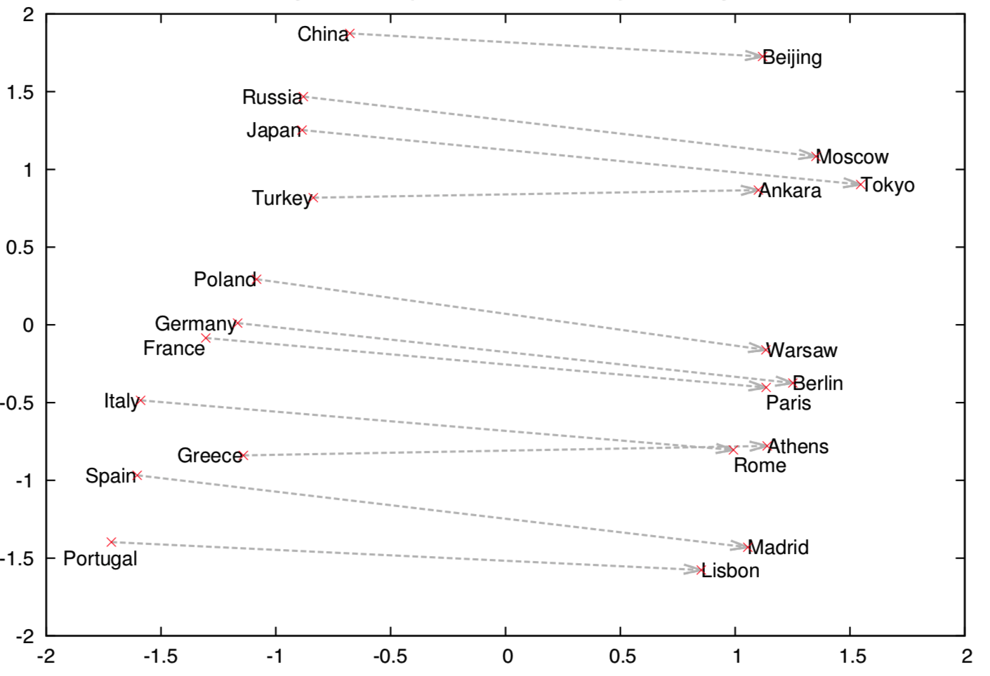
Although this model seems simple, it generates surprisingly meaningful word vectors. The embeddings represent inherent concepts and relationships between words. An example is illustrated in Figure 3.1 taken from mikolov2013distributed. It shows how the word vectors for countries and their capitals are organized, when projected onto a 2D surface using Principle Component Analysis (PCA). Another classic example is the following: king - man + woman queen. This means that if we have the vectors corresponding to king, man and woman, and if we carry out the arithmetic operation on the LHS, we get a vector which is approximately equal to the vector representation of queen. In plain English, this makes sense because a ‘king’ who is not a ‘man’ but a ‘woman’ corresponds to a ‘queen’.
Through this example of vector arithmetic, we realize how word embeddings represent semantic information. Word embeddings have been successfully applied to a wide range of NLP tasks due to their compactness (in comparison to one-hot representation) and ability to capture semantic concepts (without any explicit supervision). This study uses only word2vec embeddings and hence the details regarding other embedding models are skipped.
3.2 Sequence to Sequence LSTMs
Text generation is an important area in NLP. Introduced by sutskever2014sequence, sequence-to-sequence models have greatly benefited text generation tasks such as question answering, dialog systems and machine translation. Essentially, these models take one sequence as input and generate another sequence as output. This is in contrast to regular classification models, which output only a single class label, and not an entire sequence. models are typically implemented using two recurrent neural networks, one which is referred to as the encoder and the other is called the decoder. The encoder creates a vector representation of the input sequence that is then fed into the decoder, which then generates tokens in a sequential manner. This study uses the LSTM recurrent neural networks for encoding and decoding sentences.
More concretely, let be the tokens (i.e., the corresponding word embeddings) from the source sequence and be the tokens from the target sequence. Note that and correspond to the number of tokens (words) in the input and output sequences, respectively. At the end of the encoding process, we will have and , the final hidden and cell states respectively from the source sequence (see Section 2.2.3). We then set the initial states ( and ) of the decoder LSTM to and . This is a method to transfer information from the source side to the target side, and is known as hidden state initialization. Then, at each further timestep of the decoding process, we compute using an input word embedding (typically the groundtruth during training and the prediction from the previous timestep during testing). This is given by
| (3.2) |
where refers to the weights of the LSTM network. The predicted word at timestep is then given by a softmax layer as follows:
| (3.3) |
where is a weight matrix and the function is defined by Equation 3.4
| (3.4) |
where refers to the value of the th dimension of the output vector at timestep . In total the output vector at each timestep has dimensions, where corresponds to the vocabulary size. The layer essentially normalizes the output layer and computes a vector of probabilities. From among the dimensions of the output layer, we pick the dimension with the highest calculated probability and generate the word corresponding to that index. The operator is demonstrated with an examples in Figure 3.2.
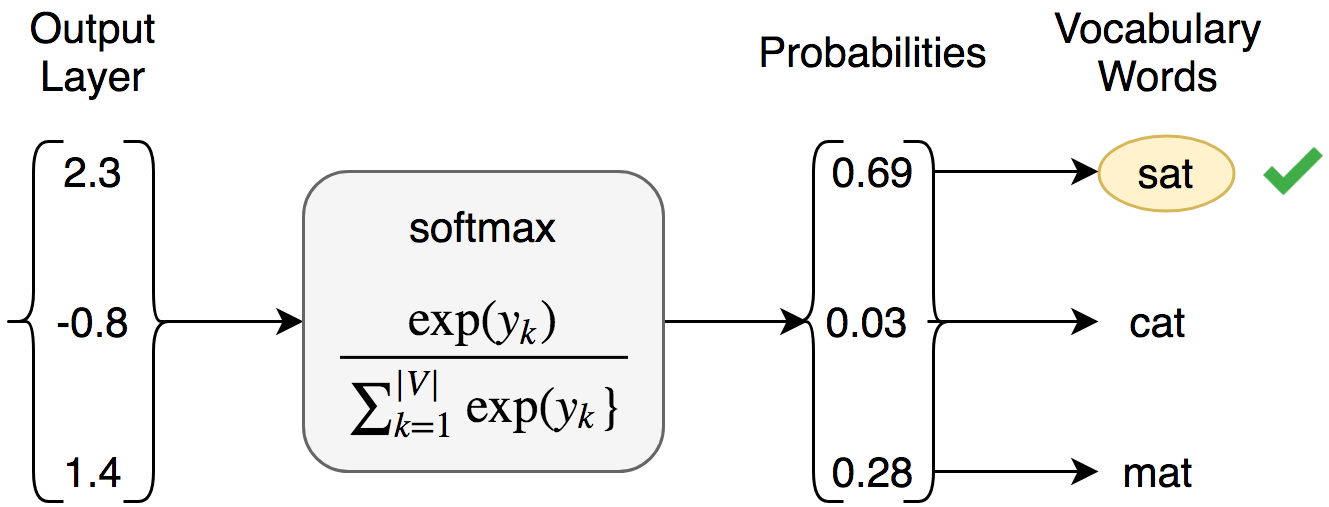
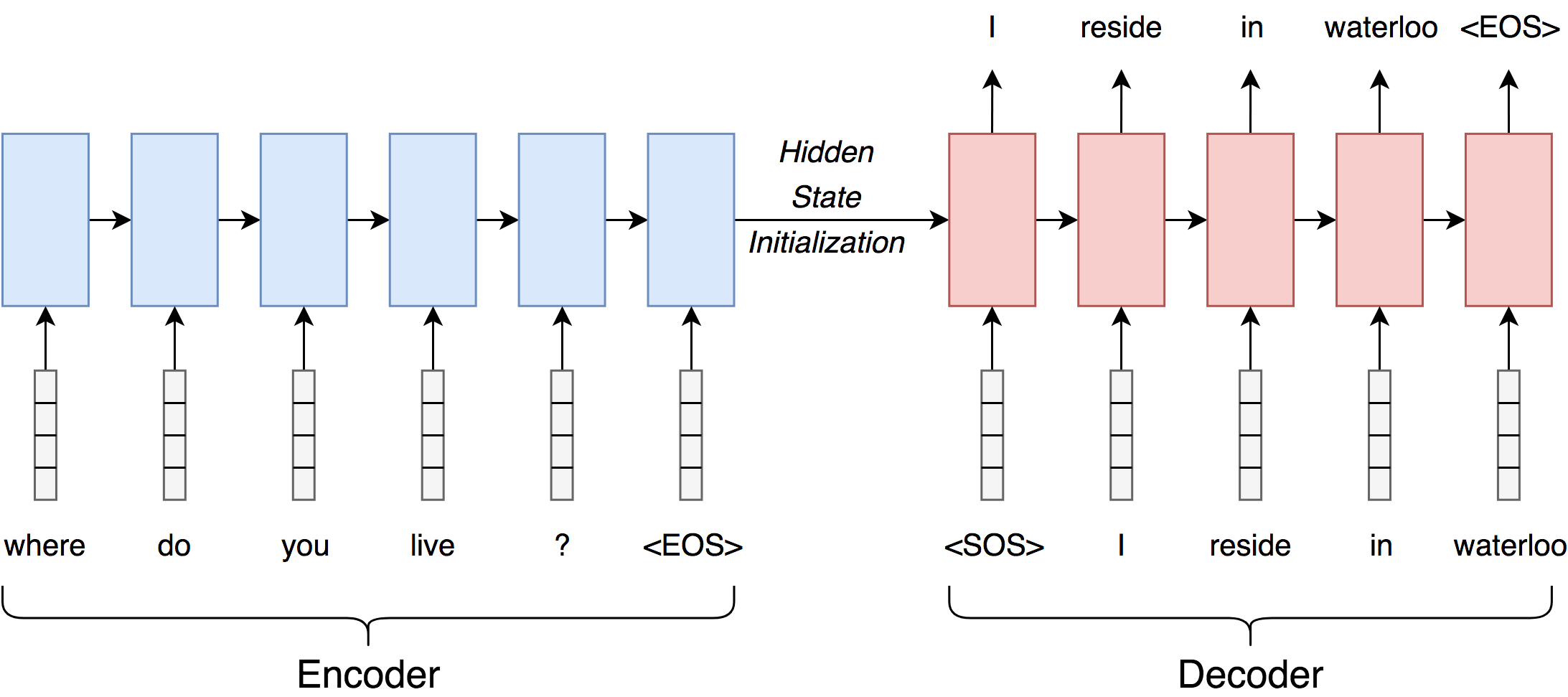
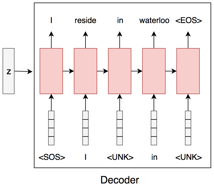
Figure 3.3 is an illustration of the working of a sequence-to-sequence LSTM model. It has a tokenized input sequence [where, do, you, live, ?] provided to the encoder LSTM. Note that the input at each timestep is the word embedding corresponding to the respective word in the vocabulary. The decoder LSTM generates the outputs [i, reside, in, waterloo]. Note the use of special tokens: (1) the start-of-sequence token <SOS>, which signals the decoder LSTM to start the decoding process; and (2) the end-of-sequence token <EOS>, which indicates when to stop decoding. The word embeddings for these can also be learnt either by pretraining the word2vec model or while training the Seq2Seq model.
3.3 Environment and Libraries
Python 3 was used as the programming environment for this project111Python Software Foundation http://www.python.org. For building word vectors, the gensim package (rehurek2010software) in Python was utilized. The deep learning models were implemented using keras (chollet2015keras) and tensorflow abadi2016tensorflow. In particular, the tf.contrib.seq2seq module was used for building encoders and decoders and calculating the loss.
Chapter 4 Variational Autoencoders
4.1 Introduction
In deep learning, autoencoders (vincent2008extracting; bengio2014deep) can be used to encode high dimensional input data into lower dimensional latent code. Variational autoencoders are a very useful class of models that combine neural networks and variational inference. In Bayesian statistics, it is common to compute posterior probability distributions. Variational inference provides a method to approximate these difficult-to-compute probability distributions through optimization. A known probability distribution of the latent code makes it possible to do generative modelling, i.e., to synthesize new samples (e.g., images) similar to the original data. In this chapter, we first provide a short introduction to variational inference. Then we describe the working of variational autoencoders including the reparameterization trick. Finally, we discuss the training difficulties associated with VAEs and empirical results obtained on a natural language dataset.
4.2 Variational Inference
Consider a latent variable model (a probability distribution over two sets of variables) given by Equation 4.1
| (4.1) |
where, refers to the observed data and the is is the latent variable. In Bayesian modeling, is known as the prior distribution of the latent variable and is the likelihood of the observation given the latent code .
The inference problem in Bayesian statistics refers to computing the posterior distribution, which refers to the conditional density of the latent variables given the data, and is given by (blei2017variational). Mathematically, this can be written as follows:
| (4.2) |
The denominator in Equation 4.2 is the marginal distribution of the data, also called the evidence. It is computed by marginalizing out the latent variables from the joint distribution .
| (4.3) |
In many cases, the evidence integral is intractable and cannot be computed in closed form (daveVI).
In Variational Inference, we obtain an approximate inference solution by trying to find an approximate distribution from a family of distributions that is similar to the posterior which we wish to estimate. In other words, we minimize the Kullback-Leibler divergence between the approximation and the true posterior distribution. The divergence (kullback1951information) is a statistical method to measure how different two probability distributions are. A lower value of divergence indicates that the distributions are more similar. It is also referred to as relative entropy. Assuming P and Q are two probability distributions, the equation for KL divergence in the discrete case is given by,
| (4.4) |
In the continuous case, this can be written as:
| (4.5) |
Returning to the discussion of variational inference, we need to find a distribution over the latent variables, namely , from a family of distributions that minimize the KL divergence with respect to the exact posterior . In equation form, this corresponds to
| (4.6) |
It is to be noted that we may get a better approximation if we choose a more complex family of distributions, at the cost of a more complex optimization process. Also, it is not possible to directly optimize Equation 4.6 since it contains the term , which was difficult to compute in the first place. Using rules of probability and logarithm, we can rewrite Equation 4.6 as follows:
| (4.7) |
Rearranging the terms, we obtain
| (4.8) |
| (4.9) |
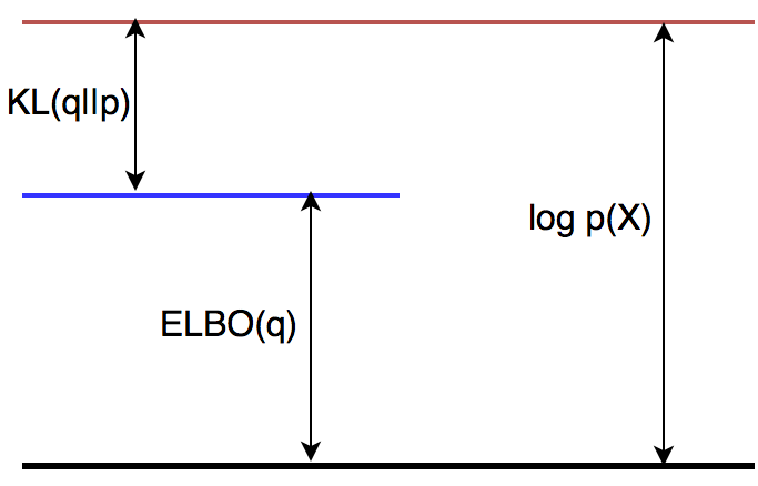
The first term on the LHS of Equation 4.8 is known as the variational lower bound (kingmathesis) The term on the RHS, , known as log evidence is constant with respect to . Since the variational lower bound is also a lower bound to the log evidence, it is also known as (yang2017understanding). That is, for any .
The LHS, which is the sum of the variational lower bound and the KL divergence adds up to a constant term on the RHS (the log probability of the observations) in Equation 4.9. Hence, the objective of minimizing KL divergence is equivalent to maximizing the variational lower bound. This is illustrated in Figure 4.1.
We can rewrite the into a simpler and more interpretable form as follows
| (4.10) |
The first term in Equation 4.10 corresponds to the expected log-likelihood of the data. The second term refers to the negative KL divergence between approximate posterior and the prior . With the overall objective to maximize , we maximize the log-likelihood while encouraging a posterior with a density function that is close to the prior.
One way to compute the approximate posterior in Equation 4.6 is using mean field inference (VI). The main assumption in the mean field variational family of distributions is that each dimension in the latent code is mutually independent and is modelled by its own density function . The optimization is carried out using Coordinate ascent mean-field variational inference (CAVI) algorithm and readers are referred to daveVI and stephanPGM for details. This thesis explores how deep learning models can be used to compute approximate posteriors, namely with the help of variational autoencoders. In comparison to traditional methods, the leverage modern neural networks and is a more powerful density estimator.
4.3 Variational Autoencoders
Introduced by kingma2013auto, variational autoencoders use neural networks to parametrize the density distributions and , discussed in Section 4.2. In theory, with sufficient layers used, neural networks can work as universal function approximators, i.e., they can be used to represent any function.
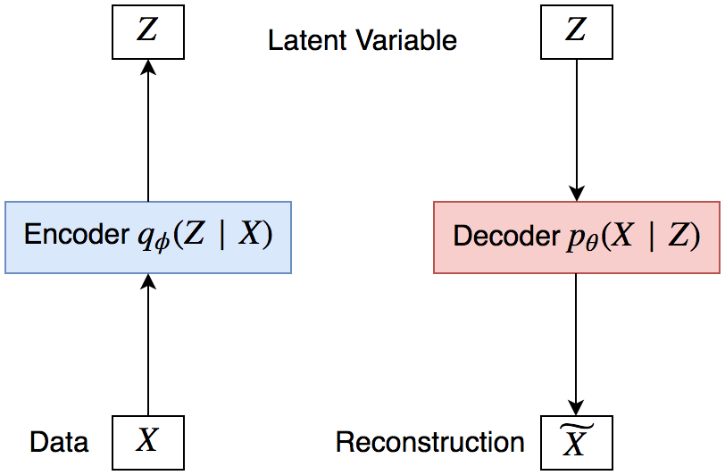
In the case of VAEs, neural networks can be used to represent the inference network (the encoder) and the generative network (the decoder) (jaanVAE; stephanPGM). To compute the approximate posterior , we can design a neural network with parameters , called the encoder . In order to reconstruct the data, we can use another neural network with parameters , which is represented as , referred to as the decoder. This is illustrated with the help of Figure 4.2. As described in Section 2.2.1, these parameters correspond to the model weights and biases.
Using the notation described above, we can replace the approximate posterior in Section 4.2 to , the one parametrized by the encoder neural network. Consider a dataset , the likelihood of a data point (log evidence) and the are related as follows:
| (4.11) |
The above equations essentially rewrite Equations 4.9 and 4.10 in the notation discussed for neural network parameterization of probability density functions. We are required to maximize the shown in Equation 4.11, which is equivalent to minimizing . The loss function for the neural network can be written as
| (4.12) |
The first term, called reconstruction loss, is the (expected) negative log-likelihood of data, similar to traditional deterministic autoencoders. For sequence-to-sequence models, this is calculated as a summation of the categorical cross entropy of the prediction across all timesteps of the decoder. The second term refers to the divergence between the approximate posterior distribution that the encoder network maps the original data space into, and the pre-specified prior. In case of continuous latent variables, the prior is typically assumed to be Gaussian . In this case, the KL divergence denoted as for input is given by the Equation 4.13 (assuming that only one sample is drawn for each input data point).
| (4.13) |
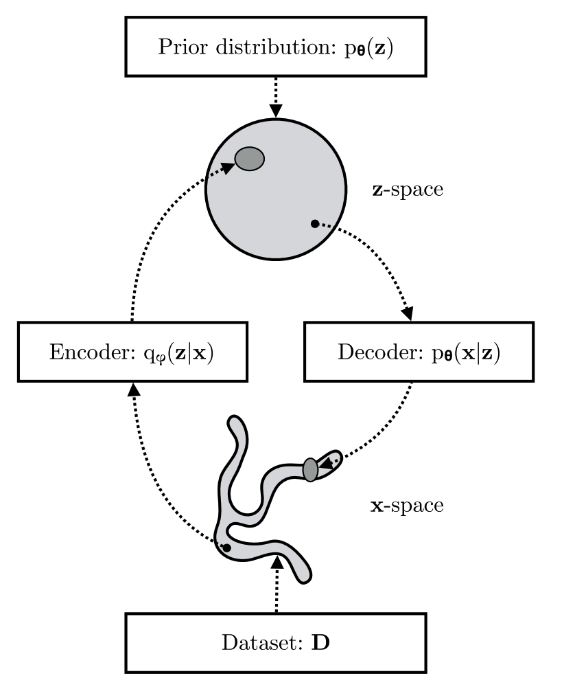
As described in doersch2016tutorial, the divergence term can be viewed as a regularization technique (similar to L2-regularization that is used to avoid overfitting). Without the term, the model boils down to a regular , that encodes the data into a latent space which can be then used for reconstruction. With the term regularization, the latent space is forced into a pre-specified distribution. As a result, the latent space now follows a known distribution, from which one can sample and synthesize new data, such as images (deep2015tejas) and sentences (bowman2015generating). This is in contrast to traditional DAEs, whose latent space can only be used for reconstruction and does not typically possess any such interesting properties. In other words, DAEs map input data onto arbitrary points on a high dimensional manifold. Whereas, VAEs project data onto continuous ellipsoidal regions that fill the latent space, rather than simply memorizing the arbitrary mappings for the input data (bowman2015generating). This is depicted in Figure 4.3, where a VAE is used to project the observed data , which has an unknown distribution, into a latent code with a known distribution (trained to be approximately similar to that of the prior by using the term regularization).
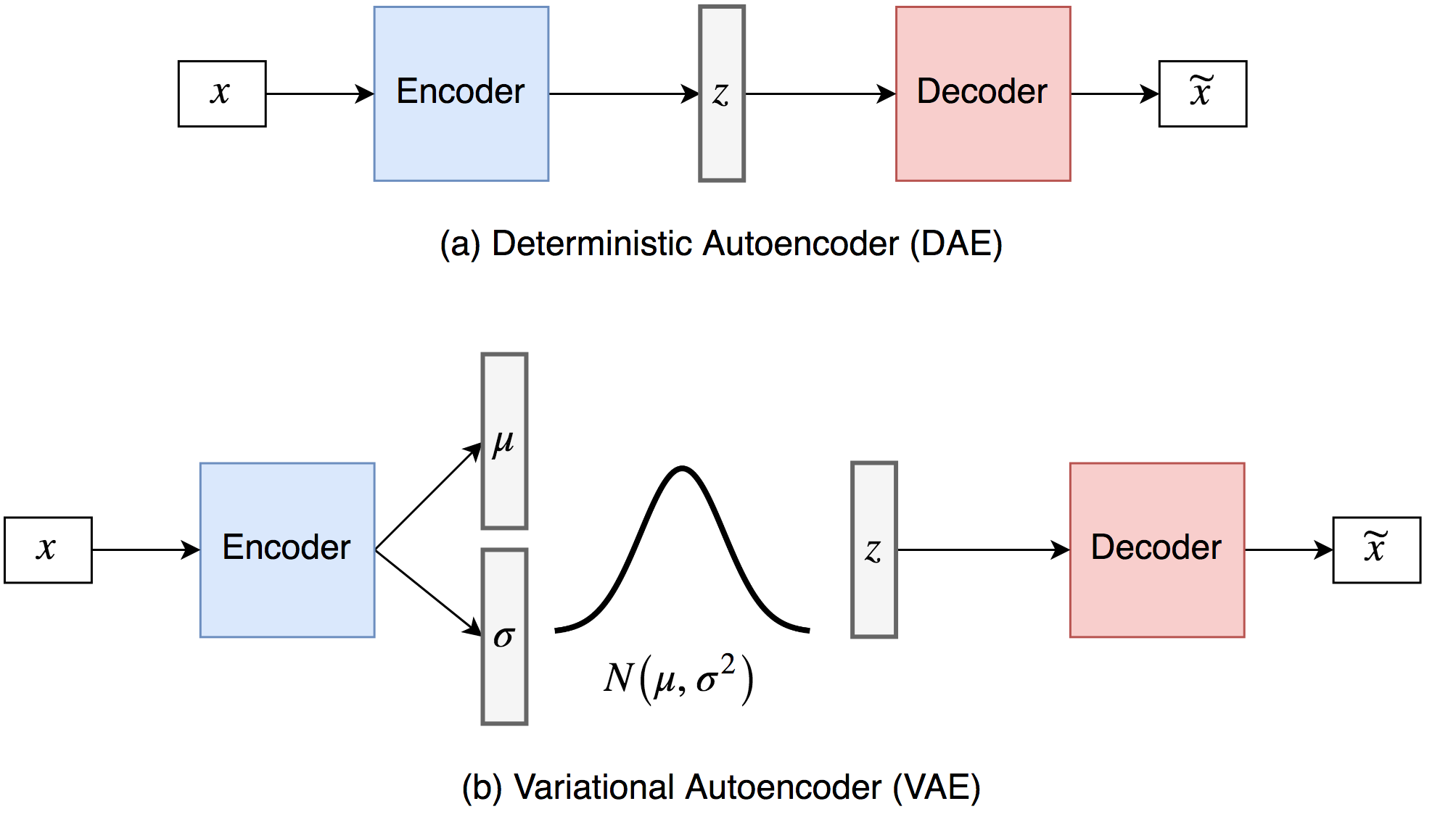
Figure 4.4 provides a comparison of the architectures for a DAE versus a VAE. In the traditional DAE, after we learn a latent code , this is directly fed to the decoder. In contrast, for VAEs, we use the encoder outputs to learn the parameters of the underlying posterior distribution. For example, if we assume Gaussian, we would want to learn its mean and variance (for simplicity we can assume a diagonal covariance matrix , which implies that the dimensions of the latent code are mutually independent). Next, we can generate a random sample from this known Gaussian distribution and feed it to the decoder. This difference in the procedure during the forward pass is demonstrated in Figure 4.4.
4.4 Reparameterization Trick
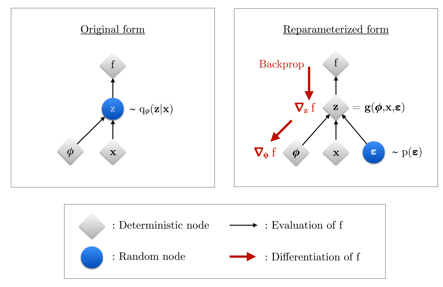
Once we have the network architecture defined, we next focus on training the model using . However, this leads to an issue because the model in its original form has a probabilistic node in the computational graph as shown in Figure 4.5. Sampling of the latent variable from the approximate posterior is carried out at the node indicated in blue on the LHS. This stochastic node results in a disconnect in the computational graph and we cannot propagate gradients back to the encoder network.
In order to circumvent this issue, kingma2013auto proposed the reparameterization trick. This simple solution involves sampling from a fixed distribution, followed by a variable transformation to the original latent space.
We can consider the example of a Gaussian distribution to illustrate the reparameterization trick. Instead of directly sampling from its posterior distribution given by , we can instead sample from and do a simple variable transformation as shown below:
| (4.14) |
where and have already been obtained by transforming the encoder output (see Figure 4.4). The effect of this reparameterization is that the gradient passes back to the encoder network (through and ) and the model is trained end to end. There is no gradient update at the node where we do the sampling of from the fixed distribution . This is exactly what we need as we do not want the fixed sampling to be influenced during gradient propagation.
4.5 Experiments
In this section, the autoencoding experiments with VAEs are detailed. We start with a description of the data and the pre-processing steps. This is followed by the training details including the optimization challenges and the strategies adopted to train the network in a stable manner.
4.5.1 Dataset
For VAE training and hyperparameter tuning, we use the Stanford Natural Language Inference (SNLI) Dataset (bowman2015large). In order to create the SNLI dataset, the authors adopted the following annotation procedure — human annotators were shown an image along with its original one-line caption; they were then asked to provide three separate sentences about the scene in the image, corresponding to the following three class labels –— entailment, neutral, and contradiction, for the task of recognizing textual entailment (androutsopoulos2010survey). The original corpus consists of 570k pairs of sentences and in this experiment, we use a randomly sampled subset of 80k sentences for training the VAE to carry out reconstruction.
4.5.2 Data Pre-processing
The following data pre-processing steps are adopted:
-
1.
All sentences are converted to lowercase.
-
2.
All punctuations except comma (,) and full stop (.) are dropped.
-
3.
We generate word2vec embeddings for all the words in the subset corpus using the CBOW model (see Section 3.1). The size of the context window was set to 5 and word embedding dimension was chosen to be 300d.
-
4.
The sentences are then shuffled and a train/validation/test split of 78k/1k/1k is created.
-
5.
Each sentence is appended with an end of sequence token EOS.
-
6.
We then decide on the vocabulary size of the model . Only the top most frequently occurring words are retained in the corpus, while the rest are replaced with a special token UNK, referring to words unknown in the vocabulary.
-
7.
Next, we tokenize sentences into a list of words using the NLTK tokenizer (bird2004nltk). Each word is then mapped into an integer index.
-
8.
Finally, we set the maximum sequence length (chosen as 10 for this experiment). Sentences with fewer than words are resized to be of size by appending a special token named PAD. Sentences with more than words are trimmed off at words.
4.6 VAE Optimization Challenges
As described in bowman2015generating, training VAEs for text generation using RNN encoder-decoder is not straightforward. Optimization challenges associated with the Kullback Leibler (KL) divergence term (between the approximate posterior and the prior) of the loss function, vanishing to zero makes the task of training VAEs notoriously difficult (bowman2015generating; yang2017improved). When the KL loss is zero, this means that the approximate posterior is exactly the same as the prior. As a consequence of this, the model fails to encode any useful information into the latent space. This causes the model to have a poor reconstruction for any given input. Hence, there is a need to balance the reconstruction term and the KL term of the loss function described in Equation 4.12. bowman2015generating suggest two strategies to overcome this issue of KL term collapse, which are adopted in this work and are described in the following subsections.
4.6.1 KL Cost Annealing
In this approach, we introduce a coefficient to the KL term of the loss function. This coefficient, referred to as the KL weight is gradually increased (annealed) from zero to a threshold value, as the training progresses. We can rewrite Equation 4.12 as follows
| (4.15) |
where refers to the KL weight, whose value is set to be a function of the iteration number during training. The key idea behind this technique is that we first allow the model to learn to reconstruct the input sentences well, and then we gradually focus on mapping the sentence encodings onto a continuous latent space by making the approximate posterior to be close to the prior. Another way to think of this annealing of the KL weight is that we gradually transform the model from a completely deterministic autoencoder into a variational one. In this study, we experimentally identify new and improved KL weight annealing schedules, which are discussed in Section 4.6.4. We find that the model is sensitive to the rate at which the KL weight is increased and the details are provided in Section 4.7.
4.6.2 Word Dropout
The other method to ensure that we learn a useful latent representation is called word dropout. As mentioned in Section 3.2, we feed the ground truth tokens delayed by one timestep to the decoder during training (see Figure 3.3). In the word dropout strategy, we replace any given input token to the decoder RNN with the UNK token with certain probability . If , the it means that no words are dropped out during decoding. On the other extreme, if we replace each word fed to the decoder with UNK. The UNK token essentially conveys no information about the source sentence (that is to be reconstructed). Referring to Figure 4.6, an example input with dropout can be [i, UNK, in, UNK], i.e., half of the words are replaced with the UNK token. Doing this weakens the decoder and encourages the model to encode more information in the latent variable to make accurate reconstructions.
4.6.3 Training Details
For training this sequence-to-sequence variational autoencoder model, we used LSTM units of dimension 100d for both the encoder and the decoder. The dimension of the latent vector was also chosen to be 100d. We adopted 300d word embeddings (mikolov2013distributed), pretrained on the 80k subset of the SNLI dataset described in Section 4.5.1. For both the source and target sides, the maximum sequence length was set to be 10. The vocabulary was limited to the most frequent 20k tokens (i.e., ). The batch size was set to be 32. Following kingma2013auto, we choose the standard normal distribution, to be the prior.
To learn the model weights, we experiment with both the stochastic gradient descent (SGD) algorithm (sgd) and the Adam optimizer (adam). For both the optimizers, a constant learning rate of 0.001 was used throughout the training process.
The model is trained for 10 epochs. We observe that the validation set converges at around 10 epochs and hence stop training further. We also compute BLEU (Bilingual Evaluation Understudy) scores on the reconstructed sentences. Originally introduced for automatic evaluation of machine translation systems, BLEU (papineni2002bleu) scores can be used to assess the sentence reconstruction capability of autoencoders. BLEU-1 measures the unigram overlap between the generated sentence and a set of reference sentences, while penalizing generated sentences that are short. In the same manner, we can determine the bigram, trigram and 4-gram overlap and report BLEU-2, BLEU-3 and BLEU-4 respectively. The automatic evaluation using BLEU scores has been reported to be correlated with human judgment (papineni2002bleu). For computing, BLEU-j based on the j-gram overlap (i.e., ), we use the following equation.
| (4.16) |
In addition to the ability of a VAE to fluently reconstruct the original input, we also need to assess the quality of the latent space created (refer Figure 4.3). This is done in a qualitative manner by randomly sampling points from the latent space and generating sentences. The exact details will be discussed in Section 4.7. A well trained VAE model should be able to generate new sentences (unseen in the training set) that are both syntactically and semantically correct.
4.6.4 VAE Variants
As mentioned in Section 4.6, training variational autoencoders for probabilistic sequence generation is not very straightforward. We try out multiple settings to train the VAE. Here, we describe and compare five VAE variants which are summarized in Table 4.1.
| VAE Variants | |
|---|---|
| ADAM-NoAnneal- | VAE trained with no KL cost annealing. The KL coefficient () is set to a constant value of 1.0 throughout training. Optimizer used is ADAM. |
| ADAM-NoAnneal- | Same setting as above, except that the is set to a constant value of 0.001 |
| ADAM-- | KL cost annealing from 0 to 3000 iterations using a rescaled tanh function (refer Eqn 4.17). Optimizer used is ADAM. |
| SGD-- | Same setting as above, but with Stochastic Gradient Descent Optimizer () |
| ADAM-linear- | KL cost annealing from 0 to 10000 iterations in a linear manner (refer Eqn 4.18). Optimizer used is ADAM. |
The models ADAM-NoAnneal- and ADAM-NoAnneal- are trained with no annealing and no word dropout. ADAM-- and ADAM-linear- have different annealing schedules, i.e., the rate and function based on which annealing is done. In ADAM--, we anneal till 3000 iterations based on Equation 4.17. At this point, the value of reaches , and we continue training with this constant till model convergence. We have a similar setting in ADAM-linear-, where the value of reaches after 10000 iterations (based on Equation 4.18) and is then kept constant for the rest of the training. For the final 3 variants in Table 4.1, word dropout was implemented as follows - at the start of training no words are dropped out () and at the end of every epoch, we increase the dropout rate by until it reaches a maximum value of . The model SGD-- is trained with the same settings as ADAM--, except that we use an SGD optimizer instead of ADAM.
| (4.17) |
| (4.18) |
where corresponds to the iteration number.
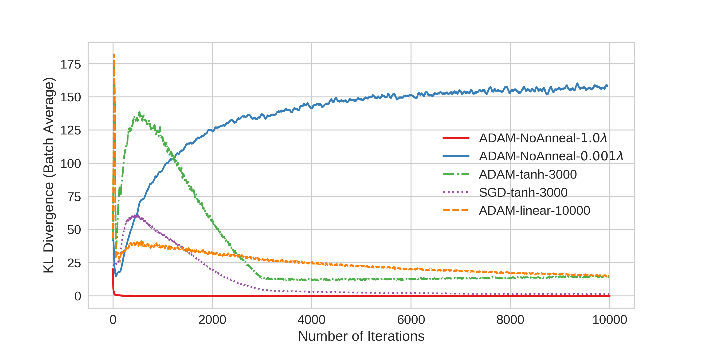
The learning curves for the different variants described earlier are illustrated in Figure 4.7. It can be seen that when there is no annealing procedure in place, the KL loss instantly vanishes to a near zero value within the first few iterations. In contrast, when , the value of is low and the model has a very small effect of the KL regularizer term. As a result, such a model tends to be more deterministic in nature.
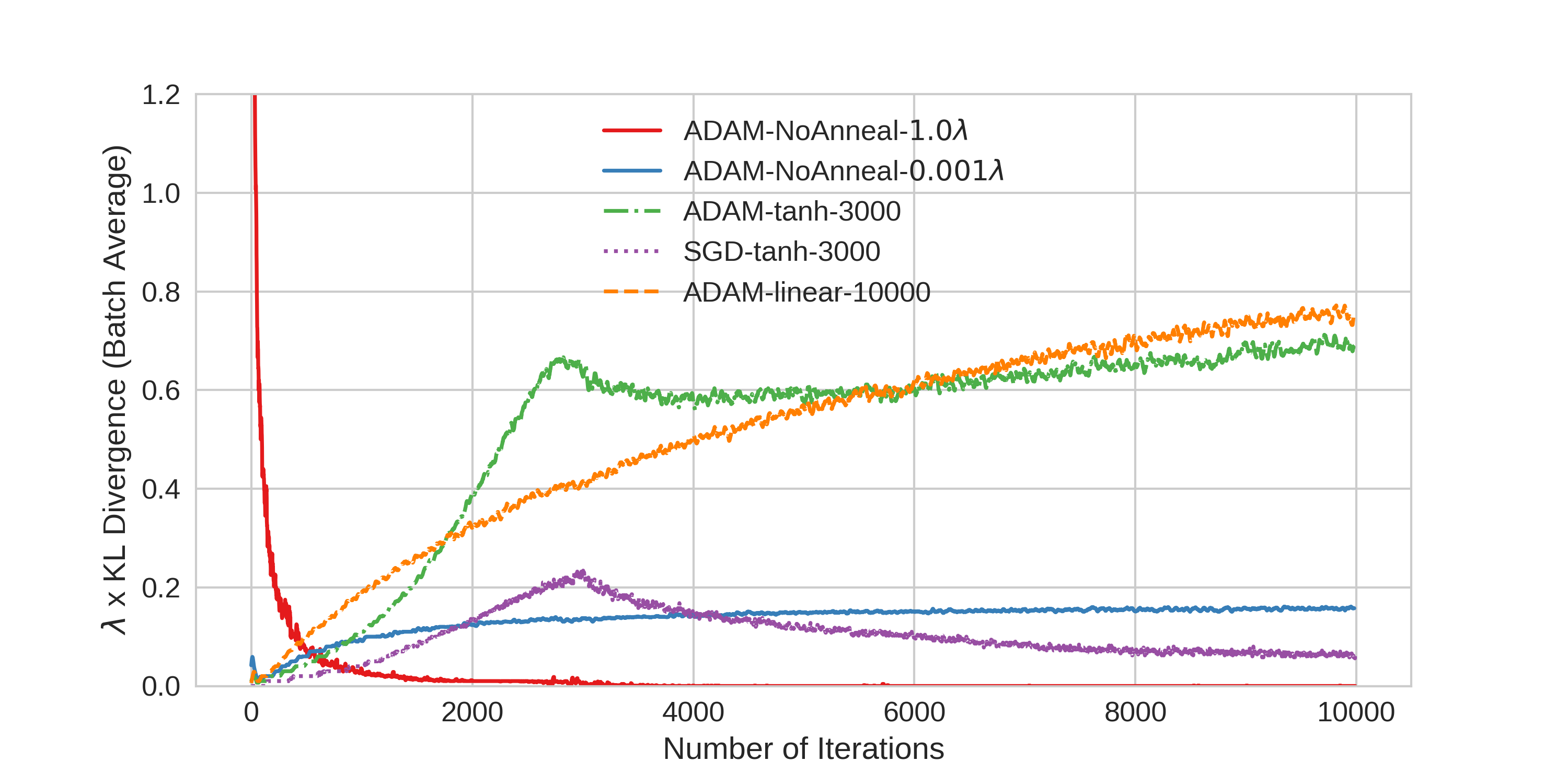
For the models that have annealing in place, the iteration till which annealing is done is an important hyperparameter. The method by which we decide the threshold value till which annealing is carried out is based on the graph. The green line in Figure 4.7 shows that beyond 3000 iterations (approximately), the value of starts to decrease after reaching a maximum value. We realize that if we do not stop annealing at this point, the KL loss steadily decreases further and collapses to zero. We determine that it is ideal to stop annealing once the value of has reached its maximum value. Beyond this point, we can continue with this constant KL coefficient for the rest of the training. For ADAM-- and ADAM-linear-, these values are 0.047 and 0.05 respectively. It can be observed that during later stages of training, the graphs for these two models tend to converge. When the optimizer is changed to SGD, a completely different pattern is observed. The reason for this unusual trend needs to be investigated further.
4.7 Results
4.7.1 Sentence Reconstruction and Random Sampling
The reconstruction performance measured in terms of BLEU scores for the different model variants are listed in Table 4.2. In this case, to generate the reconstructed sentence, we feed the mean vector () to the decoder, rather than the sampled (refer Equation 4.14). This is done so that we do not consider any variance in the latent space and pick the most probable value, the mean (referred to as the max a posteriori or MAP estimate).
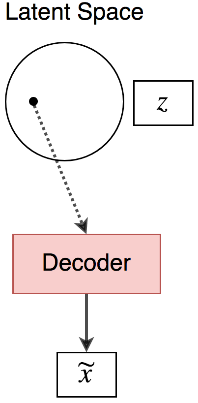
In order to assess the quality of the latent space, we randomly sample points from the prior distribution and feed the sampled to the decoder to generate new sentences. This is illustrated in Figure 4.8. If the learnt latent space is continuous, we can expect to generate a meaningful sentence by sampling from anywhere within the latent space. Note that in this setting, the encoder network can be discarded after completion of training. The randomly generated sentences for each VAE variant are shown in Table 4.3.
For comparison purposes, the BLEU scores and random sentence generations obtained using a deterministic autoencoder (DAE) are also presented. It is to be noted that while s can give better reconstructions, there is no useful latent space learnt.
The regular model trained without any optimization strategies, ADAM-NoAnneal-, produces the same output sentence irrespective of the input. This is due to the KL divergence part of the loss function collapsing to zero which causes the model to have both (1) poor reconstruction capability and (2) poor latent space.
The observation on training the model with a small constant KL coefficient of 0.001 (ADAM-NoAnneal-) is that the model tends to function like a deterministic autoencoder. This is expected since , the model ignores the KL term and becomes a deterministic autoencoder. Although the model has good reconstruction performance indicated by the high BLEU scores, its latent space is not very desirable. The sentences generated are not very meaningful and also not grammatically correct in most cases.
KL weight annealing and word dropout are indeed very useful training heuristics. This can be seen from the models ADAM-- and ADAM-linear-, both of which have sentences of similar quality being generated from the latent space. The sentences are usually syntactically and semantically correct. They are also diverse, i.e., truly random in the sense that they talk about different topics. In terms of BLEU scores, ADAM-- performs relatively better than the linear KL annealing model. However, it is to be noted that when the optimizer was changed to SGD instead of ADAM, the same model turns out to be extremely poor. The sentences generated are more or less the same, i.e., not diverse. The reconstruction capability is only slightly better than the model with the worst performance, ADAM-NoAnneal-.
By comparing ADAM-NoAnneal- and ADAM--, we realize that reconstruction performance and quality of the latent space are conflicting objectives. The model with better BLEU scores typically results in a non-continuous latent space, generating sentences of lower quality and vice-versa. If our primary objective was just sentence reconstruction, we could simply use a deterministic autoencoder, that can reconstruct sentences in a near perfect manner. From the perspective of probabilistic natural language generation by sampling from a known distribution, ADAM-- is a more desirable model.
| Model | BLEU-1 | BLEU-2 | BLEU-3 | BLEU-4 |
|---|---|---|---|---|
| Deterministic AE | 89.56 | 83.22 | 78.29 | 73.73 |
| ADAM-NoAnneal-1.0 | 26.57 | 10.32 | 4.72 | 2.05 |
| ADAM-NoAnneal-0.001 | 88.59 | 81.90 | 76.77 | 72.05 |
| ADAM-tanh-3000 | 66.97 | 53.55 | 44.36 | 36.50 |
| SGD-tanh-3000 | 32.58 | 13.74 | 6.79 | 2.70 |
| ADAM-linear-10000 | 65.55 | 52.03 | 42.98 | 35.29 |
| Deterministic AE | ADAM-NoAnneal-1.0 |
|---|---|
| a men wears an umbrella waits to | a man is sitting on a bench . |
| a couple cows a monument | a man is sitting on a bench . |
| some a play mat on the gym | a man is sitting on a bench . |
| falling bricks is checking to a tree . | a man is sitting on a bench . |
| skate other women . | a man is sitting on a bench . |
| a seagull is brown to a sandbox | a man is sitting on a bench . |
| a training underwater with the jog down the mountains | a man is sitting on a bench . |
| there is sleeping and two rug . | a man is sitting on a bench . |
| a man in a pick photos | a man is sitting on a bench . |
| a boy are people at a lake escape . | a man is sitting on a bench . |
| ADAM-NoAnneal-0.001 | ADAM-tanh-3000 |
| two men sit past where the government entering a scene | the dog is sleeping in the grass . |
| they are excited formation to ride a castle of a | the girls are being detained . |
| their janitor is leaving the dirt wearing his suits . | the group of people are going to begin . |
| two children in it exits a | a girl with blond-hair on a bike with a stick |
| six people sitting are sorting at single radio in . | a woman and a man are walking on a street |
| the guy gets cancer . | a brown dog barking at a small dog . |
| i woman who is on watch a factory | the people and a woman are giving a speech . |
| three people are wearing overalls . | the boy is competing with his athletes . |
| an artist is giving a women in china . | a biker is on the racetrack . |
| the camel is pulling on a bull . | a man wearing white racing outside . |
| SGD-tanh-3000 | ADAM-linear-10000 |
| people are playing in the street . | woman talking to the boy . |
| a man is playing a blue shirt and a blue | there are boys playing on a trampoline . |
| a man is playing in the street . | a group of people are cooking |
| a man is playing in a blue shirt . | two girls are cleaning up their beds . |
| the man is in a blue shirt and a blue | a child with bare eyes closed and being pulled by |
| the man is playing in the street . | the little girl is brushing her teeth . |
| a man is wearing a blue shirt and a blue | a few school students riding in a meadow . |
| two men are playing in the street . | the woman in the bathtub . |
| a man is wearing a blue shirt and a blue | two cyclists ride horses . |
| a man is playing in a blue shirt . | some kids are sitting . |
The ADAM-- variant has a good balance between reconstruction capability and smoothness of the latent space. Hence we adopt only ADAM-- for further discussions and evaluations. We however compare it with the deterministic autoencoder to demonstrate other interesting properties exhibited by VAEs.
4.7.2 Linear Interpolation
The objective function simultaneously minimizes the negative log likelihood of the data and the divergence between the approximate posterior distribution and the pre-specified prior. At the end of training, we can assume that the posterior and prior distributions are approximately close. This allows us to sample from the prior, which is in our case, and generate new sentences from the latent space (Section 4.7.1). If the learnt latent space is continuous, then we expect the points sampled from any part of the latent space to generate valid sentences. Another method to determine the continuity of the latent space is using linear interpolation or homotopy (bowman2015generating).
Assume that we are give two input sentences A and B. After mapping them to the latent space, we can obtain their latent representations and . For instance, we can linearly interpolate between A and B by manipulating the latent vector as follows:
| (4.19) |
where . This gives us 4 new sentences between A and B. With a good latent space, we expect the transition from A to B to happen in a smooth manner. Each linearly interpolated vector in the latent space should result in a syntactically and semantically correct sentence. The method by which linear interpolation of points in the latent space is carried out is depicted in Figure 4.9.
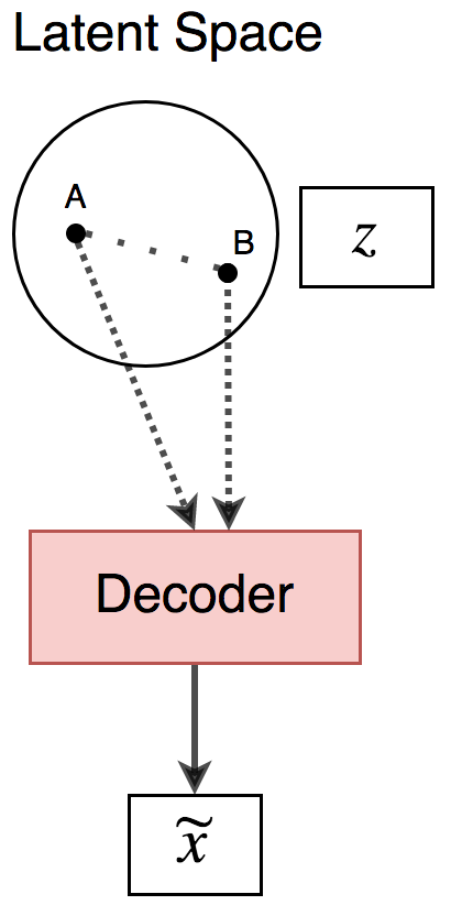
We carry out the above linear interpolation operation for both the deterministic AE and the variational AE. We can observe from Table 4.4 that in the case of the VAE, the transition is smooth. The sentences in between are both fluent and meaningful. Although, one may note that the input sentences A and B have not been perfectly reconstructed in case of the VAE. The deterministic AE on the other hand, has a better reconstruction of the original sentences. However, the intermediate sentences are not grammatically correct or meaningful. The transitions are also observed to be very irregular or non-continuous. Hence, we conclude that inclusion of the KL regularization term in the loss function of the VAE gives rise to a smooth and continuous latent space.
| Deterministic AE | VAE ADAM-tanh-3000 |
| Sentence A: there is a couple eating cake . | |
| there is a couple eating cake . | there is a couple eating cake . |
| there is a couple eating cake . | there is a couple eating . |
| there is a couple eating cake . | there is a couple eating dinner . |
| there is a group of people eating a party . | there is a couple of people eating dinner . |
| a group of men are watching a party . | a group of people are having a conversation . |
| a group of men are watching a dance party . | a group of men are having a discussion . |
| a group of men are watching a dance party . | a group of men are watching a movie . |
| a group of men are watching a dance party . | a group of men are watching a movie theater . |
| Sentence B: a group of men are watching a dance party . | |
| Sentence A: two boys are performing their fencing skills . | |
| two boys are performing their fencing skills . | two boys are performing their martial arts . |
| two boys are performing their fencing skills . | two boys are doing their homework . |
| two boys are performing their sports skills . | two boys are doing their homework outside . |
| two boys are performing chess the last . | two men are playing video games . |
| a young man is eating air inside a theater . | a young man is playing golf at a park . |
| a white man is eating alone inside a restaurant . | a young man is eating dinner in a restaurant . |
| a white man is eating alone inside a restaurant . | a young man is eating inside a restaurant . |
| a white man is eating alone inside a restaurant . | a homeless man is eating inside a restaurant . |
| Sentence B: a white man is eating alone inside a restaurant . | |
4.7.3 Sampling From Neighborhood
In a , the reparameterization trick uses the mean and standard deviation to compute the latent vector as . In other words, we sample a point in the latent space that is within one standard deviation from the mean. If we sample further away from the mean, we can expect the generated sentence to be more different from the original input which we needed to reconstruct.
In this experiment, we sample the latent vector as , i.e., within 3 standard deviations from the mean. This experiment of sampling from the neighborhood of a given input is illustrated in Figure 4.10. In a VAE, the latent space is continuous, which means that there are no empty regions. Because of this, the latent vectors sampled from any region will have meaningful representations which can be decoded into sentences. Also, since we sample not too far away from the mean, we can expect the generated sentence to have some topical similarity with the input. This can be observed from the VAE examples in Table 4.5, where for a given input, we generate sentences using multiple sampled latent vectors. Each sampled generates a different sentence, which is however topically similar to the input.
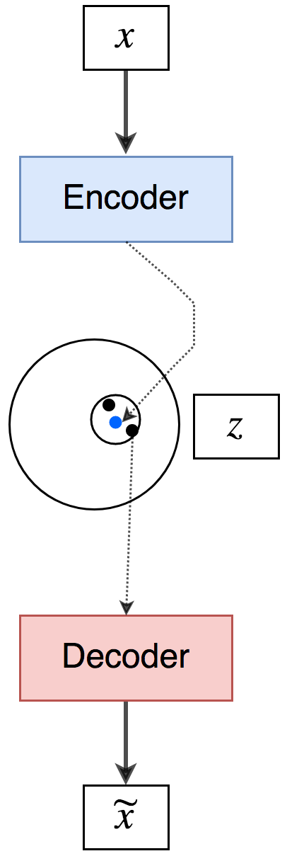
On the other hand, the deterministic autoencoder does not encode input information into a continous space. The latent space in this case is an arbitrary high dimensional manifold. As a result, when we sample points which are 3 standard deviations from the mean, we may end up in empty regions which have no useful latent encodings present. This causes the model to generate the exact same sentence which we would have obtained by feeding the mean vector to the decoder, even when multiple samples are drawn. In other words, the maps input sentences into points on the high dimensional space that are far apart with empty regions in between.
| Deterministic AE | VAE ADAM-tanh-3000 |
| Input Sentence: a dog with its mouth open is running . | |
| a dog with its mouth is open running . | a dog with long hair is eating . |
| a dog with its mouth is open running . | a guy and the dogs are holding hands |
| a dog with its mouth is open running . | a dog with a toy at a rodeo . |
| Input Sentence: the man is wearing a black suit . | |
| the man is wearing a black suit . | there are two men in a blue shirt . |
| the man is wearing a black suit . | the man is drinking from the bar . |
| the man is wearing a black suit . | the men in a black suit walking through a crosswalk . |
| Input Sentence: there are people sitting on the side of the road | |
| there are people sitting on the side of the road | the boy is walking down the street . |
| there are people sitting on the side of the road | there are people standing on the street outside |
| there are people sitting on the side of the road | the police are on the street corner . |
With the results from the 3 experiments, namely random sampling, linear interpolation and sampling from neighbourhood, we can conclude that the VAEs produce latent spaces that are continuous and characterized by a known distribution. This interesting property allows us to use VAEs for probabilistic generation of text, if trained in a careful manner.
Chapter 5 Bypassing Phenomenon
In this chapter, we discuss an important design aspect for variational neural network models. Specifically, we introduce a problem which we refer to as bypassing connection. We discuss its effects on the performance of variational autoencoders both quantitatively and qualitatively.
5.1 Problem Description
The VAE is essentially an encoder-decoder model. With the help of the learnt latent variable, the decoder can be used as a generative model . The implementation of the VAE neural network architecture consists of sampling latent vectors and feeding them to the decoder network. This has been illustrated with the help of a diagram in Figure 5.1. We use the reparameterization trick to sample from a fixed distribution and carry out a variable transformation using the learnt mean () and standard deviation ().
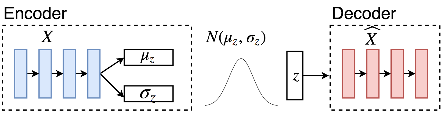
In regular sequence-to-sequence (sutskever2014sequence) models, it is common to use hidden state initialization to transfer source information to the target side. In LSTM-RNNs, this is done by setting the initial state of the decoder to the encoder’s final hidden and cell states. In the literature, the hidden state initialization technique has been extended to train VAEs (serban2017hierarchical; cao2017latent). This architecture has been illustrated in Figure 5.2. However, based on our experiments with s, we argue that such hidden state initializations results in bypassing phenomenon.
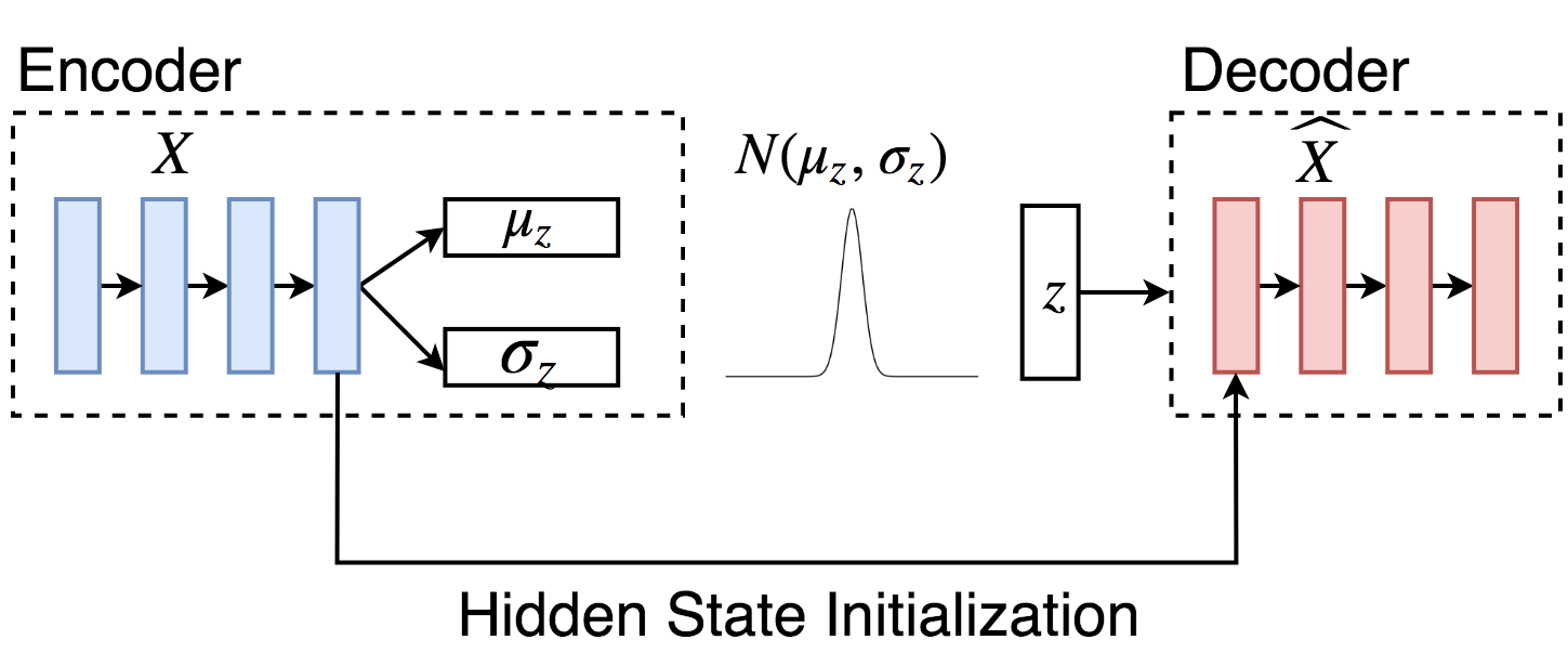
We observe that, if the decoder has a direct, deterministic access to the source information, the latent variables might not capture much information, which causes the variational space to not play a role in the training process. We call this a bypassing phenomenon. This renders the learnt latent space to be inadequate without exhibiting any variational properties such as linear interpolation and sampling from neighbourhood. The distribution of corresponding to a given input tends to be more peaked with the bypass connection (see Figure 5.2). In other words, the standard deviation around the mean is very small. As a result, sampling points around the mean, we can generate only the same or very similar sentences. In contrast, VAEs without the bypass connection can generate more diverse sentences that pertain to the same topic as the input. The latent variable distribution is flatter as depicted in Figure 5.1.
This can also be explained theoretically. Assume that is the reconstruction that needs to be generated using the latent variable . We can denote the decoder as . If the decoder is provided with a bypass connection to the source , it can now be written as . Since the latent space is much harder to learn, the decoder in this case can choose to completely ignore . It can learn to reconstruct the input just using the information from , i.e., . In this case, the reconstruction loss from Equation 4.12 can be minimized without the effect of the term. In other words, the KL term fails to act as a regularizer as it can be minimized independently by fitting the posterior to its prior. This will result in the model learning a meaningless latent space that does not encode any useful source information. Hence, a bypass connection degrades a variational model to a deterministic one. We prove this empirically in Section 5.3.
5.2 Evaluation Metrics
In a variational model, we learn a continuous latent space. We had qualitatively evaluated the latent space by random sampling and linear interpolation of sentences in Chapter 4. When provided with an input, we expect a VAE to generate sentences that are similar to the input sentence but not necessarily the exact same sentence as output. Because we sample points from around the mean vector corresponding to the input, this can result in some variability in the output. As a result, the generated sentences may be diverse, although they speak about the same topic. Here, we introduce two quantitative metrics to assess the diversity of sentences generated.
5.2.1 Entropy
Assume that for a given input , we generate outputs by sampling a new latent variable each time. We can consider this set of output sentences as our corpus and compute the unigram probability of each token. Note that the unigram probability of token is calculated by normalizing the count of that particular token by the total number of tokens in the corpus. We can compute the entropy of this unigram probability distribution as
| (5.1) |
A higher value of entropy corresponds to more randomness in the system. In our case, the that produces more diverse sentences will have a higher entropy.
5.2.2 Distinct Scores
The distinct metrics were introduced by li2015diversity for evaluating the diversity of responses provided by neural conversational agents. Similar to the case of entropy calculation, we can generate sentences for a given input. To compute Distinct-1 and Distinct-2 scores for this set of sentences, we can use the following equations.
| (5.2) | |||
| (5.3) |
The higher the distinct score, the more diverse the output sentences will be.
5.3 Results
We make use of the best performing in Section 4.7, namely the ADAM-- variant for these experiments. Specifically, we train the exact same model with and without a hidden state initialization of the decoder, which we consider a bypass connection. We observe very different learning curves for the two cases. When the model is trained with a bypass connection, the term of the loss function gradually vanishes to zero (refer Figure 5.3). In contrast, when there is no bypass connection, the can be trained in a more stable manner.
Due to the differences observed during training, we expect both models to perform differently. We employ the same technique as in Section 4.7.1 and sample points within 1 standard deviation around the mean. In this manner, we generate sentences from the latent space conditioned on a given input. We obtain diverse and topically related sentences for the with no hidden state initialization. However, the bypass connection in the other model degrades it to a deterministic autoencoder. The latent space is not continuous or smooth. This can be seen from the generated sentences in Table 5.1, which have little or no diversity.
We also verify the qualitative findings with the automatic evaluation metrics described in Section 5.2. For each input sentence in the test set, we sample 10 points in the latent space and generate 10 corresponding sentences. We then compute the entropy of each set of 10 sentences using its unigram probability distribution. The average entropy of the outputs generated by the VAE with bypass is much lower than the same model without bypass connection. Note that even a decrease in entropy of 0.68 corresponds to a relatively large difference in diversity because entropy is computed using the log-scale. The same trend is observed for the other diversity metrics, namely Distinct-1 and Distinct-2. The number of distinct unigrams and bigrams produced by the VAE without hidden state initialization is much higher than the VAE with bypass.
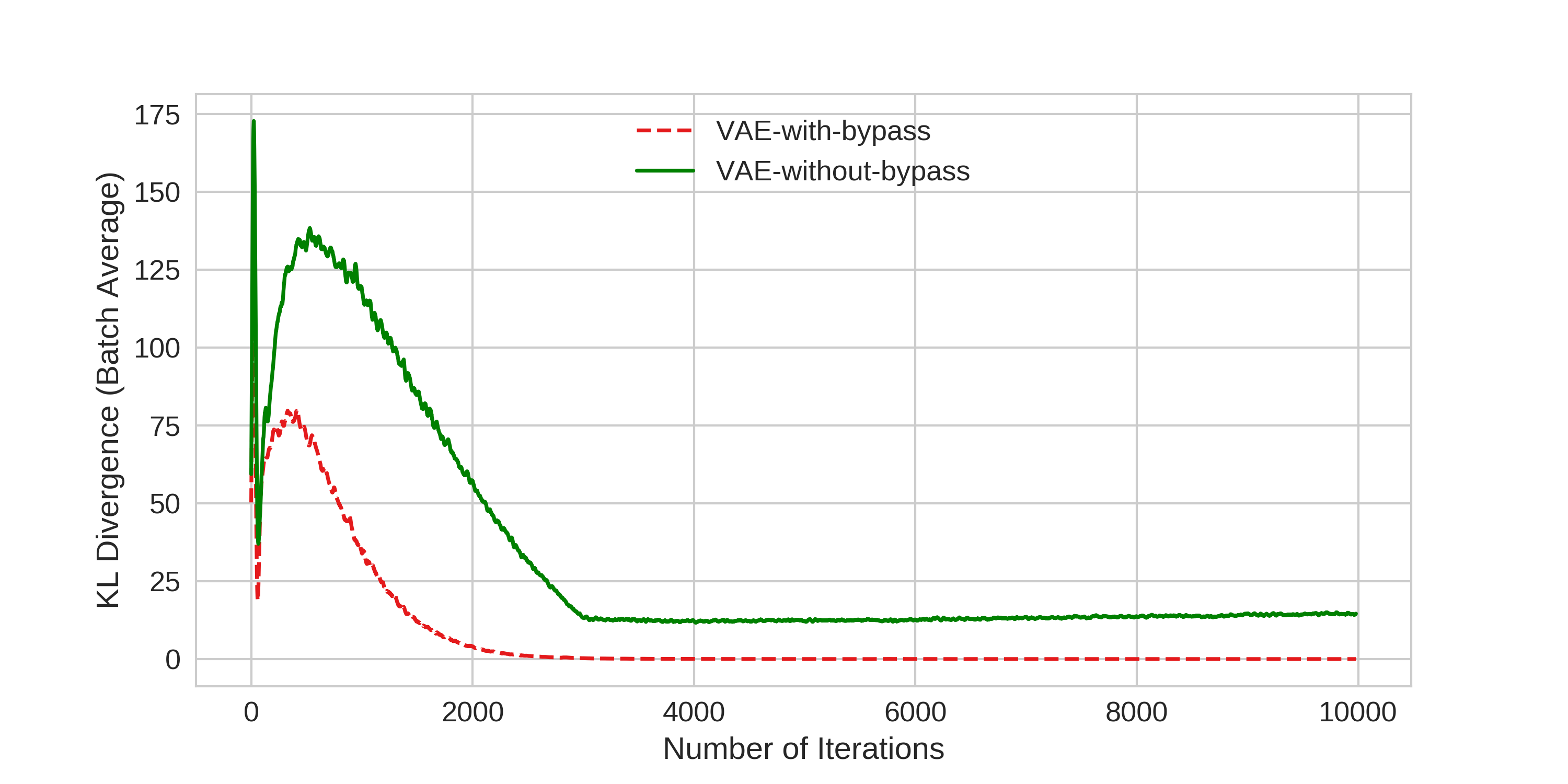
| VAE with Bypass | VAE without Bypass |
| Input Sentence: the men are playing musical instruments | |
| the men are playing musical instruments | the men are playing video games |
| the man is playing musical instruments | the men are playing musical instruments |
| the men are playing musical instruments | the musicians are playing musical instruments |
| Input Sentence: a child holds a shovel on the beach . | |
| a child holds a shovel on the beach . | a child playing with the ball on the beach . |
| a child holds a shovel on the beach . | a child holding a toy on the water . |
| a child holds a shovel on the beach . | a child holding a toy on the beach . |
| Input Sentence: a group of professional football players having a game | |
| a group of professional football players having a game | a group of football players celebrate a game |
| a group of professional football players having a game | a group of men watching a soccer match |
| a group of professional football players having a game | a group of football players having a good time |
| VAE with Bypass | VAE without Bypass | |
|---|---|---|
| Entropy | 2.004 | 2.686 |
| Distinct-1 | 0.099 | 0.302 |
| Distinct-2 | 0.118 | 0.502 |
This observation regarding the bypassing phenomenon sheds light on the design philosophy of variational neural models. This motivates us to further explore possibilities of such bypassing connections that limits the performance of variational encoder-decoder models. We discuss this in the upcoming chapters along with ways to address the issue.
Chapter 6 Variational Attention for Seq2Seq Models
6.1 Motivation
In the previous chapters, the process of autoencoding was discussed. Given an input sequence of words, the task was to learn an intermediate representation, from which it is possible to reconstruct the input. However, in most real life applications we would need to transform a given input sequence into a different output sequence. An example is the task of machine translation, where the input sentence may be in French and we would like to obtain the corresponding translated output in English. Another example is that of a conversational system, where chatbots learn to respond to user inputs.
In such scenarios, we would need to implement encoder-decoder models (rather than autoencoders). In deep learning, recurrent neural network based sequence-to-sequence models (sutskever2014sequence) are the most popular models used for text generation. They have been extensively used for machine translation (bahdanau2014neural), dialog systems (vinyals2015neural), text summarization (rush2015neural) and so on. In most cases, these models tend to be deterministic, i.e., trained to simply maximize the log-likelihood of the data.
Variational Seq2Seq models have also been applied for encoding-decoding purposes. serban2017hierarchical report that when dialog systems are trained with variational neural models, the output responses tend to be longer and more diverse. zhang2016variational show that by using variational encoder-decoder () models for neural machine translation, they achieve higher BLEU scores than existing deterministic baselines.
The introduction of attention mechanisms (bahdanau2014neural; luong2015effective) resulted in major performance improvements to existing Seq2Seq models. Attention mechanisms essentially align source information on the encoder side to target information on the decoder side. Due to this, the decoding process becomes more accurate by appropriately weighting the source information. Attention mechanisms in Seq2Seq models are described in detail in Section 6.3.
However, we argue that traditional attention mechanism cannot be directly applied to variational encoder-decoder models. Doing so unfortunately leads to bypassing phenomenon, similar to the one described in Chapter 5. In this case, deterministic attention provides direct access to the source information. This may cause the latent space to be ignored during training, resulting in an ineffective variational model. In this chapter we investigate the effect of such a bypassing connection caused by deterministic attention mechanism. We propose an alternative attention mechanism, which we refer to as variational attention that can circumvent this bypassing issue in variational encoder decoder models.
First, the traditional attention mechanism is introduced and then we discuss how this can be transformed to variational attention. Next, we report empirical results on two experiments - question generation and dialog systems. We prove the advantage of our proposed method by showing that it alleviates the bypassing phenomenon and increases the diversity of generated sentences while maintaining language fluency.
6.2 Variational Encoder Decoder
Encoder-decoder models are used when we wish to transform source information into target information . To make the model variational, we need to learn a latent variable whose distribution (referred to as the posterior) is close to a pre-specified prior. In the literature, different approaches have been proposed to learn the latent space in VEDs. zhang2016variational and cao2017latent use both and as input variables to encode information into . In this case, is sampled from a posterior distribution given by , the encoder neural network. However, this causes a discrepancy between training and prediction because is not available during the prediction stage. Hence, we follow the approach mentioned in zhou2017morphological. Here, the assumption is that can be considered as a function of , i.e., and as a result, we have . Hence, we can simply use an encoder that requires only as input to learn the latent variable . This is depicted in Figure 6.1.
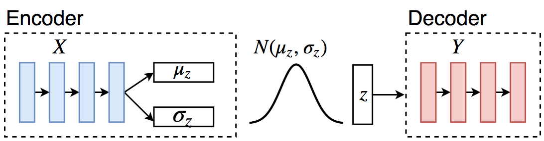
6.3 Attention Mechanism
In deep learning, attention mechanism refers to the techniques by which neural networks are trained to focus on specific aspects of the input in order to accomplish the task at hand. In this section, the attention mechanisms popularly used in models are explained. Note that this is different from visual attention in computer vision tasks such as image captioning (xu2015show) and object detection (borji2014look), which will not be covered in this thesis.
Consider s with units as both encoder and decoder. Following the same notation as in Chapter 3, let be the tokens from the source sequence and be the tokens from the target sequence. At each timestep of the decoding process, we predict the target token by computing a across the words in the vocabulary to obtain probabilities as follows
| (6.1) |
where, is a weight matrix, and is the decoder LSTM output at timestep .
| (6.2) |
where refers to the weights of the LSTM network, is the decoder input word embedding (of the output word at the previous timestep) and is the sampled latent representation of the input sentence
In , some source information is passed on to the decoder via hidden state initialization (see Section 5.1). In contrast, it is to be noted that the decoder LSTM in the vanilla Seq2Seq VED does not have access to source information other than through the latent vector . Attention mechanism can serve as a way to learn additional source information in encoder-decoder models. Essentially, during each timestep of the decoding process, the decoder is provided access to all of the encoded source tokens. More concretely, the decoder at timestep is provided with the encoder LSTM outputs, i.e., where . Now, instead of giving equal weight to every , depending on the target word to be decoded, the decoder LSTM can give higher weight to certain and lower weight to others. This means that the source outputs can be weighted differently at each decoding timestep. The idea behind this is that all source words need not contribute equally while generating the current target word.
Mathematically, attention mechanisms compute a probabilistic distribution (across the source tokens) at each decoding timestep given by
| (6.3) |
where is the weight given to source output and is a pre-normalized score. In the literature of models, two methods have been proposed to calculate .
-
1.
Multiplicative (luong2015effective)
(6.4) -
2.
Additive (bahdanau2014neural)
(6.5) where, , , and are weights that are learnt via error backpropagation.
While both methods work equally well in practice, this thesis uses the multiplicative style attention for all the encoder-decoder experiments. The next step is to take the sum of the source outputs weighted by to obtain the context vector.
| (6.6) |
Finally the attention vector can be computed using a non-linear operation and learnt weights as follows
| (6.7) |
This attention vector can now be fed to the layer at timestep . Rewriting Equation 6.1, we obtain
| (6.8) |
In this manner, attention mechanisms are capable of dynamically aligning target information to the source information, during the generation process. This process has been illustrated in Figure 6.2 and we refer to this as deterministic attention.
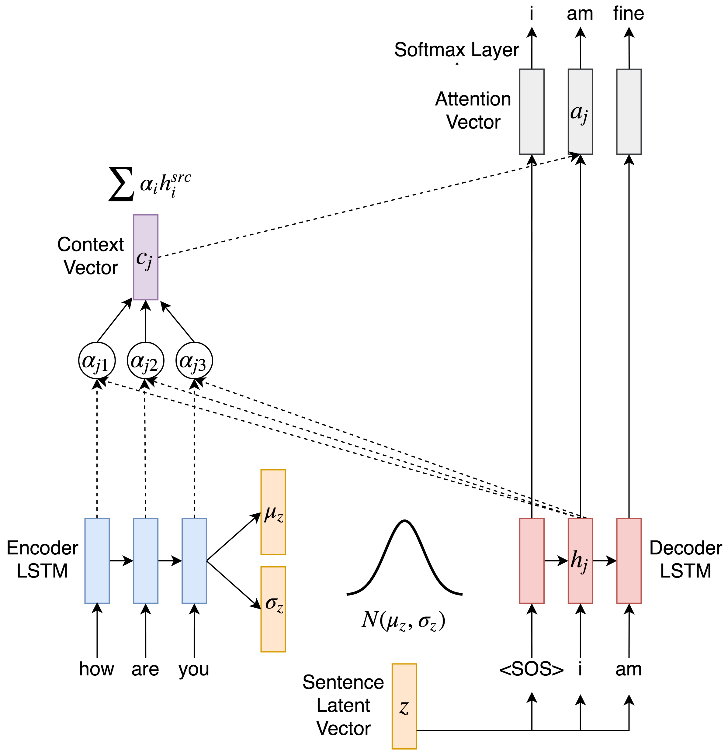
6.4 Variational Attention
One can observe from Figure 6.2, that the decoder LSTM has direct access to source information via the context vector during attention computation. Although the latent vector is fed to the decoder at every timestep, we fear that availability of source information via may cause the decoder to ignore . This may result in bypassing phenomenon due to which the model does not encode any useful information into the latent space.
In this work, we propose variational attention mechanism to prevent bypassing. Specifically, the context vector is modelled as a Gaussian random variable, which can be sampled using its mean and standard deviation. This results in a stochastic node before the layer as shown in Figure 6.3. That is, we now have two nodes in the computational graph at which we do sampling, one for the sentence latent representation and the other latent space for the context vector at every timestep . The attention is not modelled in a deterministic fashion anymore. In this way, we can prevent the bypassing issue in VED models with attention.
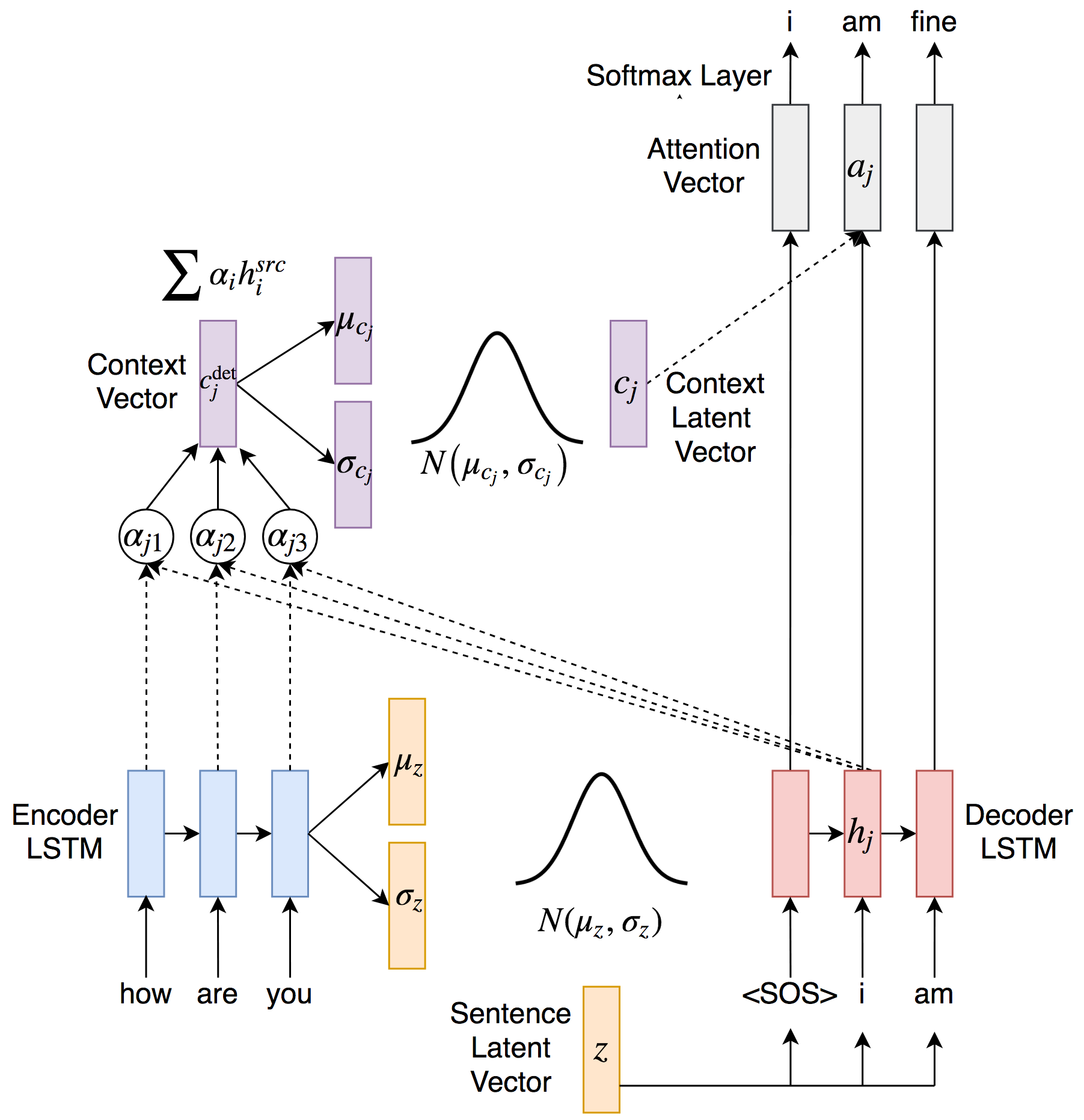
6.4.1 Derivation of Loss Function
Variational attention treats both the sentence representation and the context vector as random variables. We would need to regularize the distribution of both these latent variables in the loss function. Analogous to the case of , we rewrite Equation 4.11 for evidence lower bound () by adding the extra variable . The ELBO for the th timestep of the th data point, i.e., input and target , can be expressed as follows.
| (6.9) |
where and correspond to the encoder and decoder neural networks with respective weights and . Given , we can assume conditional independence between and . Hence, the posterior factorizes as . We also assume separate priors for and . In this way, the sampling procedure can be done separately and the loss can also be computed independently.
| (6.10) |
As mentioned in Chapter 4, we are required to maximize the evidence lower bound, which is equivalent to minimizing . The first term then becomes the negative log-likelihood, which can be computed as the standard Seq2Seq word prediction categorical cross-entropy loss, summed across all timesteps (). Next, we have two KL regularization terms - one for the sentence latent space and the other for the context vector at each timestep . In both cases, we are required to minimize the KL divergence between the computed posterior and the pre-specified prior. Hence, the overall training objective of the Seq2Seq with both variational sentence latent space and variational attention is to minimize the following loss function,
| (6.11) |
In the above equation, acts as coefficient of both the terms. We only anneal this hyperparameter in a manner similar to that of the as discussed in Section 4.5. is the coefficient of the context vector’s KL term which is kept constant throughout training. This is done because training variational models can be difficult and we would like to anneal just one of the coefficients which can simultaneously influence both KL terms.
Prior
Similar to the VAE described in Chapter 4, the sentence latent code is assumed to have a standard normal prior . For the context vector , we propose two plausible priors:
-
1.
The simplest option would be to set the prior to be .
-
2.
With an understanding of attention mechanism in Seq2Seq models, one can observe that is calculated as a linear combination of the source hidden states, i.e., . Geometrically, this means that the context vector is inside the convex hull of hidden representations of the source sequence, i.e., . Thus, we choose as an alternative choice for the prior, where , the mean of the source hidden states.
Posterior
Once we have pre-specified the prior distributions of both latent variables and , we now discuss how the corresponding approximate posteriors are computed. In both cases, an based encoder neural network is used to parameterize the posterior distributions. More concretely, for the sentence latent space, the encoder’s final hidden state is linearly transformed to obtain and , the parameters of the posterior Gaussian distribution. Now the posterior of can be defined as .
In an analogous manner, the posterior of the context vector at timestep , denoted by is modeled as a Gaussian distribution using the same encoder neural network. We first compute the context vector in a deterministic manner () as mentioned in Equation 6.6 and then transform it into the variational space using learnt parameters and . For the mean , we apply an identity transformation, i.e., . To compute , we first transform by a neural layer with activation followed by another linear transformation. We can then sample the context vector from its posterior . Readers are referred to Figure 6.3 for a diagrammatic overview of the method in which the parameters of the posterior distributions are computed.
6.5 Experiments
In this section, we provide the