The Main Belt Asteroid Shape Distribution from Gaia Data Release 2

Abstract

Gaia Data Release 2 includes observational data for 14,099 pre-selected asteroids. From the sparsely sampled $G$ band photometry, we derive lower-limit lightcurve amplitudes for 11,665 main belt asteroids in order to provide constraints on the distribution of shapes in the asteroid main belt. Assuming a triaxial shape model for each asteroid, defined through the axial aspect ratios $a>b$ and $b=c$, we find an average $b/a=0.80\pm 0.04$ for the ensemble, which is in agreement with previous results. By combining the Gaia data with asteroid properties from the literature, we investigate possible correlations of the aspect ratio with size, semi-major axis, geometric albedo, and intrinsic color. Based on our model simulations, we find that main belt asteroids greater than 50 km in diameter on average have higher $b/a$ aspect ratios (are rounder) than smaller asteroids. We furthermore find significant differences in the shape distribution of main belt asteroids as a function of the other properties that do not affect the average aspect ratios. We conclude that a more detailed investigation of shape distribution correlations requires a larger data sample than is provided in Gaia Data Release 2.

1 Introduction

Asteroid physical properties provide important constraints on the formation and evolution of our Solar System, including clues to the different phases of orbital instability and migration of the giant planets (see, e.g., Morbidelli et al., 2015). Collisions within the asteroid belt can play a major role altering the asteroid population. These clues are recorded in the shapes of individual asteroids, so that a global understanding of the shape distribution — as informed by a large catalog — provides insight into our Solar System’s evolution.

Shape information can be determined for individual asteroids from photometric data over a long period of time, with Doppler-delay radar imaging, with ground-based adaptive optics techniques, or in situ via spacecraft data. These last three techniques are limited in the number of targets that can be reasonably observed. As a result, only a small percentage of km-scale main belt asteroids have known shapes and spin-pole orientations. For instance, the DAMIT database (Ďurech et al., 2010) holds information for less than 1,000 asteroids as of writing this. Currently, the predominant method for determination of asteroid shape and spin properties is the inversion of dense photometric lightcurves, as initially developed by Kaasalainen & Torppa (2001) and Kaasalainen (2001). Without dense photometric data it is difficult to derive detailed shape and spin pole orientations for individual asteroids. With a sufficiently large dataset, however, it is possible to determine a statistical shape distribution, even if only a small number of data points are present for each individual asteroid. The advantage of a large untargeted dataset is that it provides an estimate for a population’s shape distribution without being subject to observational biases in favor of elongated objects (i.e., higher lightcurve amplitudes) that are commonly present in targeted observations. Previous work on the shape distribution for main belt asteroids (MBAs) has been carried out by McNeill et al. (2016), Cibulková et al. (2016), Nortunen et al. (2017), and Cibulková et al. (2018).

European Space Agency’s Gaia astrometric space observatory (Prusti et al., 2016) measures the positions, distances, proper motions, and other physical properties of more than one billion stars in our galaxy with unprecedented accuracy. In addition to its main mission, Gaia will also observe a significant fraction of the currently known asteroid population (${\sim}$350,000 Solar System small bodies) and discover previously unknown asteroids (Spoto et al., 2018). The sample of Gaia-observed asteroids provides a large uniform and magnitude-limited set of observations perfectly suited to independently investigate the distribution of asteroid shapes.

2 Gaia Data Release 2

Gaia Data Release 2 (DR2, Spoto et al., 2018) includes 1,977,702 astrometric observations of 14,099 pre-selected asteroids, observed between 5 August 2014 and 23 May 2016. Solar System moving objects are identified through association with known asteroids with well-defined orbits. The majority of DR2 asteroids are main belt asteroids, but the sample also includes a small number of Near-Earth Asteroids, Jupiter Trojans, and trans-Neptunian objects. Each “transit” of a target across the detector array leads to 9 individual detections across a typical time span on the order of 40 s. Target positions and epochs are provided for individual detections, whereas photometric information is averaged per transit. Photometric information on asteroids in DR2 is limited to Gaia $G$ band (0.33–1.0 $\mu$m) magnitudes, fluxes, and flux uncertainties.

3 Data Analysis

3.1 Data Preparation

All DR2 asteroid observations were downloaded from CDS Vizier. Since the photometry per object is the average of all individual observations within a single transit, we extract only the midtime epoch from each transit. The maximum number of transits for any individual object is 53 and the median number of transits per target is 9. We require a minimum of 5 transits per object to be considered in this analysis. While this criterion is somewhat arbitrary, it allows for a meaningful statistical analysis of the data set, which is not guaranteed for a smaller number of observations. For each transit, we derive approximate $G$ band magnitude uncertainties from the provided fluxes and flux uncertainties. We obtain ephemerides for the respective epochs and relative to Gaia using the astroquery.jplhorizons module, which queries ephemerides from the JPL Horizons system (Giorgini et al., 1996). For each $G$ band observation, we derive the reduced $G$ band magnitude, $G_{11}(\alpha)$, which corrects for geometric effects as a result of the heliocentric distance of the target, $r$, and the distance from the observer, $\Delta$, but preserves the solar phase angle ($\alpha$) dependence of the brightness: $G_{11}(\alpha)=G-5\log_{10}r\Delta$. We remove all objects that are not considered main belt asteroids from our sample since the population sizes of near-Earth asteroids, Jupiter Trojans, and trans-Neptunian objects in DR2 are insufficient for this analysis. Our final sample consists of 121,819 $G$ band photometric observations of 12,059 different main belt asteroids.

3.2 Phase Correction and Amplitude Measurement

Variations in the $G_{11}(\alpha)$ magnitudes are the result of lightcurve variations due to the irregular shapes of asteroids and their rotation, as well as solar phase angle effects (see, e.g., Bowell et al., 1989). In order to extract shape information from the data, the phase angle effect has to be corrected for. On average, DR2 observations span a phase angle range of 6° around an average phase angle of 19°, which is insufficient to perform a reliable phase curve fit. In order to correct for solar phase angle effects on the Gaia photometry, we instead use existing phase curve information on our targets from Vereš et al. (2015) and Oszkiewicz et al. (2011). While Vereš et al. (2015) only used photometric observations obtained by Pan-STARRS1 (Kaiser et al., 2010), Oszkiewicz et al. (2011) compiled low-precision photometric data from the Minor Planet Center (MPC). Both sources make use of the $H$-$G_{12}$ two-parameter phase function (Muinonen et al., 2010) and provide measured absolute magnitudes ($H$) and slope parameters ($G_{12}$) with corresponding uncertainties. Preference is given to slope parameters reported by Vereš et al. (2015) if their measurement is based on at least 5 observations; this selection is based on the improved reliability and existence of photometric uncertainties in the Pan-STARRS1 data in contrast to the MPC data. If no measurement from Vereš et al. (2015) is available, we adopt the slope parameter reported by Oszkiewicz et al. (2011). In our final sample, 56% of the $G_{12}$ slope parameters were taken from Vereš et al. (2015) and 44% were taken from Oszkiewicz et al. (2011). Only 24 targets in our sample had no measurement of the slope parameter $G_{12}$ from neither Vereš et al. (2015) nor Oszkiewicz et al. (2011); these targets were rejected from our further analysis.

Based on the solar phase angles during the Gaia observations and the slope parameter $G_{12}$ from the literature, we correct the $G_{11}(\alpha)$ magnitudes for phase angle effects, resulting in normalized $H_{G}$ absolute magnitudes that reveal the targets’ lightcurve variations. In order to account for uncertainties in the derivation of the slope parameter $G_{12}$, we adopt a Monte Carlo approach in which we vary $G_{12}$ using a Gaussian model based on the $G_{12}$ uncertainties reported by Vereš et al. (2015) or Oszkiewicz et al. (2011); the latter source utilizes asymmetric uncertainties, which we adopt throughout this work. We vary $G_{12}$ using two different Gaussian distributions corresponding to the upper and lower 1$\sigma$ uncertainties, re-derive the magnitude offsets and $H_{G}$ values, and calculate the weighted standard deviation (we use the inverse square uncertainties of the Gaia photometry as weights) of the resulting $H_{G}$ magnitudes. We adopt the average of the weighted $H_{G}$ standard deviations from 1,000 Monte Carlo runs as the target’s lightcurve amplitude. This method tends to underestimate large lightcurve amplitude, especially in the case of sparse data; our derived amplitudes $A$ hence represent lower limits of the real lightcurve amplitudes (see Section 5.2 for a discussion). Figure 1 shows an example of the method that we use to derive lightcurve amplitudes. Finally, we use a linear regression model (scipy.stats.linregress) to identify objects with strong linear slopes in their $H_{G}$ magnitudes as a function of solar phase angle, which are most likely caused by incorrect phase slope parameters $G_{12}$. Objects with coefficient of determination parameters $r^{2}>0.5$ or $p$-values less than 0.05 are rejected as they unanomously point to severe sloping. These criteria are somewhat arbitrary and result from the visual inspection of a few hundred objects. However, they provide a conservative rejection scheme.

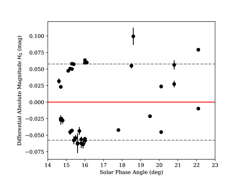
Figure 1: Example lightcurve amplitude derivation for asteroid (79) Eurynome. The diagram shows differential absolute magnitudes in $G$ band ($H_{G}$) derived using the method defined in Section 3.2 and plotted against solar phase angle. These differential magnitudes are obtained by subtracting the weighted average $H_{G}$ from the individual measurements to better visualize the scatter around the target’s normalized average absolute magnitude (red line). We drive the lower limit lightcurve amplitude (peak-to-peak) as two times the standard deviation (dashed lines) of this scatter. In the case of Eurynome, we derive a lower limit amplitude of 0.10 mag from 36 DR2 observations. The Asteroid Lightcurve Database (Warner et al., 2009) lists a maximum lightcurve amplitude of 0.25 mag, which is consistent with our lower limit. The sloping of the $H_{G}$ magnitudes as a function of solar phase angles suggests that the adopted $G_{12}$ photometric slope parameter does not describe the target’s phase curve well in this particular case. The linear regression analysis for this data set yields a coefficient of determination parameter $r^{2}=0.003$ and a $p$-value of 0.75, which does not lead to a rejection of this object from our sample (see Section 3.2).

4 Results

For each DR2 target, we derive the lower limit lightcurve amplitude using the method introduced in Section 3. The results for all 11,665 main belt asteroids for which this method succeeded (84.3% of the complete DR2 sample; 98.6% of the main belt asteroids in the sample with sufficient data as defined in Section 3.1) are listed in Table 1.

Table 1: DR2 Main Belt Asteroid Lightcurve Amplitudes and Auxiliary Data

MPC	Amp.	$N_{\mathrm{obs}}$	Phase Angle		Slope Parameter				SDSS Color	$a$	Diameter	Albedo
Number	(mag)		Min (°)	Max (°)	$G_{12}$	$\sigma_{+}$	$\sigma_{-}$	Source	$a^{\text{*}}$	(au)	(km)	$p_{V}$
8	0.15	8	17.2	28.2	0.33	0.08	-0.08	o	…	2.201	158.4	0.21
33	0.11	26	12.5	26.3	0.15	0.53	-0.53	v	…	2.876	50.9	0.24
280	0.11	27	14.3	22.3	0.38	0.31	-0.31	v	-0.04	2.942	55.8	0.03
460	0.10	8	17.2	20.7	0.32	0.11	-0.11	o	0.09	2.717	19.7	0.26
11644	0.13	7	12.2	17.4	-0.41	0.31	-0.31	v	0.01	3.118	13.4	0.09
…	…	…	…	…	…	…	…	…	…	…

Semi-major axis of the target as obtained from the Minor Planet Center database in astronomical units.

Asteroid diameter as derived by Mainzer et al. (2016) in kilometers.

Asteroid geometric albedo ($V$ band) as derived by Mainzer et al. (2016).

Note. — This table is only a representative excerpt and is published in its entirety in the machine readable format. A portion is shown here for guidance regarding its form and content.

4.1 Asteroid Shape Distribution

In order to derive the average shape distribution of main belt asteroids, we implement the model used by McNeill et al. (2016). This model generates a synthetic population of asteroids with random shapes and spin pole orientations and compares them to the observed data using a $\chi^{2}$ goodness of fit test. Shapes are generated assuming a triaxial ellipsoidal shape with axis ratios $b/a$ and $b/c$; we generate random ratios $0.2\leq b/a<1.0$ and presume $b=c$. We assume the spin pole latitudes and longitudes of the observed objects based on the distribution for small (diameter ${\leq}30$ km) asteroids obtained by Hanuš et al. (2011); spin frequencies are derived from a uniform distribution covering 1–10.9 day^-1, corresponding to rotational periods ranging from the spin barrier at 2.2 h to a period of 24 hr. This assumption is consistent with the flat distribution of measured rotational frequencies at small sizes (Pravec et al., 2002). We account for phase angle variations in each target by assigning monotonically increasing or decreasing phase angle values based on the ensemble properties of DR2 targets (see Section 3.2 and Table 1). We furthermore account for the fact that lightcurve amplitudes measured as part of this work represent lower limits by increasing each measured amplitude by 51% and adding a noise contribution following a normal distribution with a relative standard deviation of 20% in each Monte Carlo run. This approach is justified in Section 5.2.

Based on 10,000 Monte Carlo runs using 11,665 synthetic objects each, we find an average aspect ratio for main belt asteroids $b/a=0.80\pm 0.04$. The nominal value is defined as the global minimum $\chi^{2}$ of all model runs; the uncertainty is derived within a reasonable range ($\chi^{2}\leq 2$) around the global minimum of the distribution. We discuss this result in Sections 5.1 and 5.3.

4.2 Trends and Correlations

We investigate potential correlations between our derived lightcurve amplitudes and intrinsic target properties: semi-major axis, color, albedo, and diameter. For this analysis, we match our sample target list with previously derived asteroid color parameters $a^{\text{*}}$ (Ivezić et al., 2001) from the Sloan Digital Sky Survey (SDSS) Moving Object Catalog (Data Release 3, Ivezić et al., 2005), diameters and albedos of WISE-observed small bodies (Mainzer et al., 2016), as well as semi-major axes as provided by the Minor Planet Center database. We use sbpy.data.Names.parse_asteroid to parse the respective asteroid identifiers in the different archives to perform the object matching. The SDSS color parameter $a^{\text{*}}$ is derived as the average over all available measurements; in order to reject outliers, we restrict ourselves to the range $-0.3<a^{\text{*}}<0.3$. Similarly, WISE diameters and albedos are derived as averages if multiple observations are available.

Matching objects and measured properties are listed in Table 1 and plotted in Figure 2. Aspect ratios ($b/a$) have been derived from the lower limit amplitudes $A$ using the relation $b/a=10^{-0.4\cdot A}$. We furthermore repeat the analysis performed in Section 4.1 for sub-samples that are defined based on the respective parameter distributions. The sub-sample definitions and average aspect ratio results are listed in Table 2. In order to derive the latter, we use the exact same model as described in Section 4.1 but applied to the individual sub-samples.

Table 2: Sub-Sample Definitions and Average Aspect Ratios

Parameter	Range	Description	$N_{\mathrm{obj}}$	Average Aspect Ratio ($b/a$)
Semi-major axis ($a$)	$a<2.5$ au	inner main belt	4,054	$0.79\pm 0.03$
	$2.5\leq a<2.82$ au	middle main belt	3,880	$0.79\pm 0.03$
	$a\geq 2.82$ au	outer main belt	3,731	$0.79\pm 0.03$
Intrinsic Color ($a^{\text{*}}$)	$a^{\text{*}}<0$	blueish asteroids	1,008	$0.79\pm 0.03$
	$a^{\text{*}}\geq 0$	reddish asteroids	2,547	$0.79\pm 0.03$
Diameter ($d$)	$d<10$ km	small asteroids	5,821	$0.79\pm 0.03$
	$10\leq d<50$ km	medium-sized asteroids	3,673	$0.80\pm 0.03$
	$d\geq 50$ km	large asteroids	468	$0.86\pm 0.05$
Geometric Albedo ($p_{V}$)	$p_{V}\leq 0.1$	primitive asteroids	2,827	$0.80\pm 0.03$
	$p_{V}>0.1$	non-primitive asteroids	7,135	$0.79\pm 0.03$
—	—	all main belt asteroids	11,665	$0.80\pm 0.04$

We find no significant differences in the average aspect ratios derived from our model (see Section 4.1) in sub-samples based on intrinsic color, semi-major axis, and geometric albedo. However, we find a difference in the average aspect ratio between medium-sized asteroids and large asteroids (see Table 2 for definitions) at the $1\sigma$ level: our model suggests that main belt asteroids with diameters ${\geq}50$ km are rounder than smaller asteroids, which agrees with trends from previous studies (Cibulková et al., 2016; Nortunen et al., 2017; Cibulková et al., 2018).

We also use a $k$-sample Anderson-Darling test (scipy.stats.anderson_ksamp) to investigate differences in the amplitude distributions in the individual sub-samples. We find the null-hypothesis that the different subsamples in semi-major, object diameter, intrinsic color, and object albedo come from the same distribution can be rejected at the 1% level. This indicates clear differences in the amplitude distributions as a function of these parameters, which do not affect the average aspect ratios derived from our model (see Figure 2). More detailed studies will be possible with the availability of a better coverage of the asteroid population with Gaia Data Release 3.

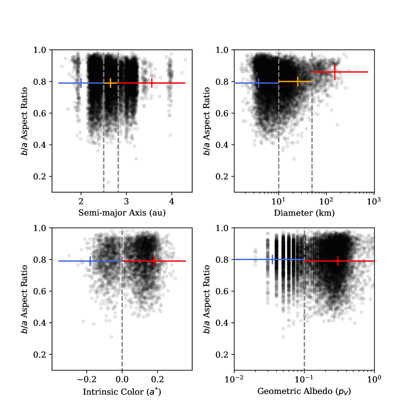
Figure 2: Correlations of the $b/a$ aspect ratios measured in this work with other target properties from the literature: semi-major axis (top left), target diameter (top right), intrinsic color (bottom left), and geometric albedo (bottom right). Semi-transparent dots represent individual objects. The colored error symbols represent the average $b/a$ aspect ratio per sub-population as indicated by the vertical dashed lines (compare to Table 2).

5 Discussion

5.1 Comparison to previous work

We compare our derived mean aspect ratio for main belt asteroids ($b/a=0.80\pm 0.04$) with previous results. McNeill et al. (2016) derived the average triaxial shape parameters of main belt asteroids with diameters ${\leq}20$ km from Pan-STARRS1 observations as ($1:0.85\pm 0.13:0.71\pm 0.12$; this value has been updated to $1:0.83\pm 0.07:0.70\pm 0.06$ with the updated form of the model which now more accurately accounts for phase angle amplitude correction), which agrees within the uncertainties with our findings for the same size regime. Cibulková et al. (2016) find aspect ratios $b/a={\sim}0.63$ for main belt asteroids with diameters smaller than 25 km and $b/a={\sim}0.77$ for main belt asteroids greater than 50 km from the Lowell photometric database (Bowell et al., 2014). Both results are lower than our estimates – implying a higher average elongation of the targets – although the general trend of larger objects being rounder is consistent with our results. This effect might be caused by the large individual photometric uncertainties (0.1–0.2 mag) of the data sample used in that work, which might overestimate lightcurve amplitudes (Cibulková et al., 2018). Nortunen et al. (2017) use dense photometric observations (e.g., from WISE, Wright et al., 2010), finding probability density functions for the triaxial shape parameters that agree with our result for asteroids with diameters greater than 50 km, but they also find asteroids smaller than 50 km to be more elongated ($b/a{\sim}0.55$) than in this work. This discrepancy might point to an albedo-based selection bias in our sample of optically observed asteroids that is not existent in the WISE sample that affects this measurement. Detailed modeling of this bias and the underlying elongation distributions will be necessary to confirm this hypothesis, which we defer to the future when we can make use of a larger number of Gaia-observed main belt asteroids. Finally, based on a prolate spheroidal shape model ($a\geq b=c$) and Pan-STARRS1 photometric data, Cibulková et al. (2018) find $b/a\sim 0.8$ for main belt asteroids with diameters greater than 12 km, which also agrees with our result.

5.2 Validation of our approach

We compare our lower-limit amplitudes against previously measured amplitudes cataloged in the Asteroid Lightcurve Database (LCDB, Warner et al., 2009), restricting ourselves to the most reliable information from that source (uncertainty parameter $U$=3). The amplitude comparison is plotted in the top panel of Figure 3. We find a significant fraction of small-amplitude ($A_{\mathrm{LCDB}}\leq$0.25 mag) targets to have overestimated amplitudes. This effect is at least in part caused by incorrect phase slope parameters $G_{12}$, which can lead to an artificial sloping of the derived $H_{G}$ magnitudes as a function of solar phase angle and hence lead to an overestimation of the lightcurve amplitude. Additional effects may include amplitude modulations as a function of a target’s observer-centric ecliptic longitude (see Bowell et al., 2014, and Section 5.3 for a discussion). For larger amplitudes ($A_{\mathrm{LCDB}}>0.25$ mag) the comparison shows a clear underestimation of large amplitudes on our side. This effect is caused by the incomplete sampling of the target’s lightcurve. We quantify this underestimation by fitting a linear slope to the data shown in Figure 3 (top). Based on this fit, we find that we underestimate the lightcurve amplitudes by 51%; the scatter of the data points with respect to this slope is 20%, providing a measure of uncertainty for an individual object after applying the average 51% correction. We use these findings in Section 4.1 to correct our derived lower-limit lightcurve amplitudes. The bottom panel of Figure 3 shows that this offset is independent of the number of observations per target. However, we find amplitudes derived from many observations to be more reliable.

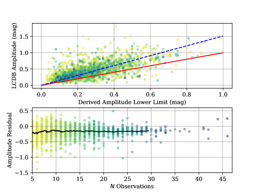
Figure 3: Top: Comparison of derived lower-limit lightcurve amplitudes and previously derived lightcurve amplitudes from the Asteroid Lightcurve Database (LCDB, Warner et al., 2009). The red line indicates unity; the blue dashed line represents a linear fit to the scatter cloud. The colors of the points corresponds to the color scheme used in the bottom panel. Bottom: Amplitude residuals (this work minus LCDB) as a function of the number of observations per target. The black line indicates a running average over 100 adjacent data points.

5.3 Limitations of this Analysis

This analysis is limited by a number of simplifications. In our derivation of the lightcurve amplitudes of our targets (Section 3.2) we ignore the effect of the solar phase angle on the lightcurve amplitude. From the limited amount of DR2 observations, we are unable to account for this effect on a per-object basis. Instead, we investigate the magnitude of this effect on the ensemble of measured lightcurve amplitudes using the relation derived by Zappalà et al. (1990) and an assumed average phase slope parameter of 0.02 mag/degree together with the average solar phase angle in our sample (19°). Based on these assumptions, we expect our lightcurve amplitudes to be overestimated by 40%. However, in Section 5.2, our comparison of the lightcurve amplitudes derived in this work with previously measured lightcurve amplitudes from the literature shows that we are on average underestimating lightcurve amplitudes. We interpret this discrepancy as a sign that the effect of the solar phase angle on the lightcurve amplitude is insignificant for our ensemble analysis.

Furthermore, the spin pole orientations of the majority of our sample targets are unknown. For individual objects, this lack of information can be critical in two ways: (1) the relative orientation of the spin pole axis to the observer directly modulates the observed lightcurve amplitude in a geometrical effect, and (2) the orientation of the spin poles axis introduces additional variability that can exceed the target’s lightcurve amplitude as a function of the observer-centric ecliptic longitude (see, e.g., Bowell et al., 2014).

We justify the use of the spin pole distribution derived for asteroids smaller than 30 km (Hanuš et al., 2011) in our model (Section 4.1) with the fact that the majority of our sample objects with measured diameters fall into this size regime (${\sim}$90%). Nevertheless, we investigate the impact of this choice on the results and redo the analysis in Section 4.1 based on a uniform distribution of spin poles in both ecliptic latitude and longitude. This distribution agrees with the distribution for larger asteroids (Hanuš et al., 2011) and represents the extreme opposite to our original choice, allowing us to probe any differences in the results. The resulting average aspect ratios for all samples agree with our nominal results within their 1$\sigma$ uncertainties. This observation is supported by the results of a Kolmogorov-Smirnov test (e.g., Press et al., 1992) in which we compare the de-biased amplitude distributions generated in our model based on the different spin pole distributions and find no significant differences between those distributions.

Finally, we assume in our derivation of the average aspect ratios that the $b$ and $c$ axis ratios of our asteroids will be equal. Shape models from dense light curve inversion are the only existing data sets which can detail the relationship between these axes. These data, however, are incomplete and likely to be biased toward higher $b/c$ values. Allowing $b/c$ to vary will slightly inflate the value obtained for the $b/a$ axis ratio but not to an extent greater than the uncertainties produced by the model.

6 Conclusions

We measure lower limit lightcurve amplitudes for 11,665 main belt asteroids in the Gaia Data Release 2 catalog. We derive the mean aspect ratio for main belt asteroids as $b/a=0.80\pm 0.04$, which is in agreement with previous studies. We investigate trends in the shape distribution as a function of semi-major axis, intrinsic color, diameter, and geometric albedo, using data from the literature. Based on our model simulations, we find that main belt asteroids greater than 50 km in diameter have on average higher $b/a$ aspect ratios (are rounder) than smaller asteroids. We furthermore find significant differences in the derived lower limit amplitude distributions with respect to semi-major axis, intrinsic color ($a^{*}$), and geometric albedo. We predict that more detailed population and shape distribution studies will be possible with the availability of Gaia Data Release 3.

References

- Astropy Collaboration et al. (2013) Astropy Collaboration, Robitaille, T. P., Tollerud, E. J., et al. 2013, A&A, 558, A33
- Bowell et al. (1989) Bowell, E., Hapke, B., Domingue, D. et al. 1989, Asteroids II, Tucson, AZ, University of Arizona Press, 1989, 524
- Bowell et al. (2014) Bowell, E., Oszkiewicz, D. A., Wasserman, L. et al. 2014, M&PS, 49, 95
- Cibulková et al. (2016) Cibulková, H., Ďurech, J., Vokrouhlický, D. et al. 2016, A&A, 596, A57
- Cibulková et al. (2018) Cibulková, H., Nortunen, H., Ďurech, J. et al. 2018, A&A, 611, 86
- Ďurech et al. (2010) Ďurech, J., Sidorin, V., Kaasalainen, M. 2010, A&A, 513, A46
- Giorgini et al. (1996) Giorgini, J. D., Yeomans, D. K., Chamberlin, A B. et al. 1996, Bulletin of the American Astronomical Society, 28, 1158
- Hanuš et al. (2011) Hanuš, J., Ďurech, J., Brož, M. et al. 2011, A&A, 530, A134
- Ivezić et al. (2001) Ivezić, Ž., Tabachnik, S., Rafikov, R. et al. 2001, AJ, 122, 2749
- Ivezić et al. (2005) Ivezić, Ž., Jurić, M., Lupton, R. H. et al. 2005, NASA Planetary Data System, id. EAR-A-I0035-3-SDSSMOC-V2.0
- Jones et al. (2001) Jones E., Oliphant E., Peterson P., et al. SciPy: Open Source Scientific Tools for Python, 2001-, http://www.scipy.org/, accessed 2018-06-13
- Kaasalainen & Torppa (2001) Kaasalainen, M., Torppa, J. 2001, Icarus, 153, 1, 24
- Kaasalainen (2001) Kaasalainen, M. 2001, A&A, 376, 302
- Kaiser et al. (2010) Kaiser, N., Burgett, W., Chambers, K. et al. 2010, In: Stepp L.M., G. R., H.J., H. (Eds.), Ground-based and Airborne Telescopes III, Volume 7732 of Proceedings of the SPIE, pp. 77330E–77330E–14
- Mainzer et al. (2016) Mainzer, A. K., Bauer, J. M., Cutri, R. M. et al. 2016, NASA Planetary Data System, id. EAR-A-COMPIL-5-NEOWISEDIAM-V1.0
- McNeill et al. (2016) McNeill, A., Fitzsimmons, A., Jedicke, R. et al. 2016, MNRAS, 459, 3, 2964
- Morbidelli et al. (2015) Morbidelli, A., Walsh, K. J., O’Brien, D. P. et al. 2015, Asteroids IV, Patrick Michel, Francesca E. DeMeo, and William F. Bottke (eds.), University of Arizona Press, Tucson, 493
- Muinonen et al. (2010) Muinonen, K., Belskaya, I. N., Cellino, A. et al. 2010, Icarus 209, 2
- Nortunen et al. (2017) Nortunen, H., Kaasalainen, M., Ďurech, J. et al. 2017, A&A, 601, A139
- Oszkiewicz et al. (2011) Oszkiewicz, D. A., Muinonen, K. et al. 2011, J. Quant. Spectrosc. Radiat. Trans. 112, 1919
- Pravec et al. (2002) Pravec, P., Harris, A. W., Michalowski, T. 2002, Asteroids III, W. F. Bottke Jr., A. Cellino, P. Paolicchi, and R. P. Binzel (eds), University of Arizona Press, Tucson, 113
- Press et al. (1992) Press, W. H., Teukolsky, S. A., Vetterling, W. T., Flannery, B. P. 1992, Numerical recipes in C. The art of scientific computing, Cambridge: University Press, 2nd ed.
- Prusti et al. (2016) The Gaia Collaboration, Prusti, T., de Bruijne, J. H. J., Brown, A. G. A. et al. 2016, A&A, 595, A1
- Spoto et al. (2018) Spoto, F., Tanga, P., Mignard, F. et al. 2018, A&A, 616, A13
- Vereš et al. (2015) Vereš, P., Jedicke, R., Fitzsimmons, A. et al. 2015, Icarus, 261, 31
- Warner et al. (2009) Warner, B. D., Harris, A. W., Pravec, P. 2009, Icarus 202, 134, Updated 2017-11-12 http://www.MinorPlanet.info/lightcurvedatabase.html
- Wright et al. (2010) Wright, E. L., Eisenhardt, P. R. M., Mainzer, A. K. et al., 2010, AJ, 140, 1868
- Zappalà et al. (1990) Zappala, V., Cellino, A., Barucci, A. et al. 1990, A&A, 231, 548