Langevin Simulations of a Long Range Electron Phonon Model

Abstract

We present a Quantum Monte Carlo (QMC) study, based on the Langevin equation, of a Hamiltonian describing electrons coupled to phonon degrees of freedom. The bosonic part of the action helps control the variation of the field in imaginary time. As a consequence, the iterative conjugate gradient solution of the fermionic action, which depends on the boson coordinates, converges more rapidly than in the case of electron-electron interactions, such as the Hubbard Hamiltonian. Fourier Acceleration is shown to be a crucial ingredient in reducing the equilibration and autocorrelation times. After describing and benchmarking the method, we present results for the phase diagram focusing on the range of the electron-phonon interaction. We delineate the regions of charge density wave formation from those in which the fermion density is inhomogeneous, caused by phase separation. We show that the Langevin approach is more efficient than the Determinant QMC method for lattice sizes $N\gtrsim 8\times 8$ and that it therefore opens a potential path to problems including, for example, charge order in the 3D Holstein model.

I Introduction

Quantum Monte Carlo (QMC) constitutes one of the most powerful non-perturbative approaches to interacting fermion Hamiltonians. Its applications have led to insight into both renormalized single particle properties at low density, and also to many-body phase transitions in systems ranging from high energy, to nuclear, to condensed matter physics. Nevertheless, fermion QMC suffers from several serious limitations: (i) Algorithms generally scale as the cube of the number of particles or sites, a consequence of the evaluation of the determinants arising when the fermionic degrees of freedom are integrated out. (ii) Depending on the model and on the parameter regime, long autocorrelation times can also challenge the calculations. Finally, (iii) the fermion sign problem remains the most restrictive bottleneck in the field.

Considerable progress has been made in addressing (i) in the lattice gauge theory (LGT) community, e.g. with linear scaling methods for the fermion determinant evaluation. However, these techniques have proven surprisingly difficult to carry over into condensed matter (CM) and specifically to the Hubbard model scalettar86 ; scalettar87 ; yamazaki09 ; bai09 ; beyl18 . The general belief is that the difficulty arises from two related problems: the high degree of anisotropy between imaginary time ($\beta$) and the spatial dimensions present in CM problems, as opposed to the relativistic LGT case, and the much more rapid variation of the Hubbard-Stratonovich field configurations in the imaginary time direction which gives rise to less well-conditioned matrices. The eigenvalue spread in CM problems leads to large conjugate gradient iteration counts, and, indeed, often, to a complete absence of convergence of iterative matrix inversion solvers.

In this paper we explore the application of linear scaling QMC methods to electron-phonon Hamiltonians. We are motivated by the fact that, in such models, the kinetic energy terms $\sum_{i}\hat{p}_{i}^{2}/2$ in the oscillator Hamiltonian smooth the imaginary time variation of the phonon field. As a consequence, the condition number of the fermion determinants is likely to be improved relative to that which arises in the Hubbard model, where the Hubbard-Stratonovich field has no similar dynamics. It is for the latter case that most of the linear scaling methods have previously been tested scalettar86 ; scalettar87 ; yamazaki09 ; bai09 and shown to be effective only in a limited parameter regime of weak coupling and/or relatively high temperature.

The successful application of Langevin methods to electron-phonon models would be a considerable step forward, since their physics holds significant intrinsic interest. Early QMC work focused on the dilute limit. As an electron moves through a material, the polarization of the underlying medium causes a cloud of phonons to follow. Simulations studied the resulting “single electron polaron”, identifying its size and effective mass as functions of the electron-phonon coupling and phonon frequency kornilovitch98 ; kornilovitch99 ; alexandrov00 ; hohenadler04 ; ku02 ; spencer05 ; macridin04 ; romero99 ; bonca99 ; chandler14 . If the interaction $\lambda$ is sufficiently large, two polarons can pair with a bipolaron size and dispersion which depend on $\lambda$hague09 .

Meanwhile, as the density increases, QMC has explored how local up and down spin pairs, which form due the effective interaction mediated by the lattice distortion, can arrange themselves spatially into charge density wave (CDW) patterns, especially on bipartite latticesscalettar89 ; noack91 ; niyaz93 . The critical temperatures of transitions to long range order phases have been evaluatedweber17 ; costa18 . These CDW patterns typically induce insulating behavior, and compete with superconducting phases which can also occur if the pairs become phase coherent across the latticescalettar89 ; costa18 .

In the remainder of this paper, Sec. 2 will describe the specific Hamiltonian to be studied, its experimental motivation, and the details of the Langevin method. Section 3 contains benchmarks of our results and comparisons with other methods. Section 4 describes results for the low temperature ordered phases of the Hamiltonian, and Sec. 5 presents some concluding remarks.

II Model and Methods

We will study the properties of a two-dimensional system governed by the Hamiltonian,

$$\hat{H} =\hat{H}^{0}_{\rm el}+\hat{H}^{0}_{\rm ph}+\hat{V}_{\rm el-ph},$$ (1)

$$\hat{H}^{0}_{\rm el} =-t\sum_{\langle ij\rangle\sigma}\big{(}\,\hat{c}_{i\sigma}^{\dagger}\hat{c}_{j\sigma}^{\phantom{\dagger}}+\hat{c}_{j\sigma}^{\dagger}\hat{c}_{i\sigma}^{\phantom{\dagger}}\,\big{)}-\mu\sum_{i\sigma}\hat{n}^{\phantom{\dagger}}_{i\sigma},$$

$$\hat{H}^{0}_{\rm ph} =\frac{1}{2}\,\omega_{0}^{2}\,\sum_{i}\hat{x}_{i}^{2}+\frac{1}{2}\,\sum_{i}\,\hat{p}_{i}^{2}\,\,,$$

$$\hat{V}_{\rm el-ph} =\lambda_{0}\sum_{ir\sigma}f(r)\,\hat{x}_{i}\,\hat{n}_{i+r,\sigma},\hskip 15.89948ptf(r)=\frac{e^{-r/\xi}}{(1+r^{2})^{3/2}}.$$

$\hat{c}_{i\sigma}^{\dagger}$ and $\hat{c}_{j\sigma}^{\phantom{\dagger}}$ are creation and destruction operators for electrons of spin $\sigma$ on lattice site $i$, so that $\hat{H}^{0}_{\rm el}$ describes the hopping of electrons of spin $\sigma$ between near neighbor sites $\langle ij\rangle$. Here we focus on a 2D square lattice and choose $t=1$ to set the energy scale. $\hat{H}^{0}_{\rm ph}$ represents a dispersionless (optical) phonon mode on each lattice site. In $\hat{V}_{\rm el-ph}$, the phonon displacement $\hat{x}_{i}$ on site $i$ couples to the electron densities $\hat{n}_{i+r,\sigma}$ with a strength $\lambda_{0}f(r)$ which falls off exponentially with separation $r$frohlich54 . Our simulations are done in the grand-canonical ensemble, with a chemical potential $\mu$ which couples to the fermion density $\hat{n}^{\phantom{\dagger}}_{i\sigma}=\hat{c}^{\dagger}_{i\sigma}\hat{c}^{\phantom{\dagger}}_{i\sigma}$. The model has a particle-hole symmetry on a bipartite lattice; half-filling is attained at $\mu=-(\sum_{r}\lambda(r))^{2}/\omega_{0}^{2}$. In the literature, $\hat{V}_{\rm el-ph}$ is sometimes written by replacing $\hat{x}_{i}\rightarrow(\,\hat{a}^{\dagger}_{i}+\hat{a}^{\phantom{\dagger}}_{i}\,)/\sqrt{2\omega_{0}}$ and defining the coupling $g=\lambda_{0}/\sqrt{2\omega_{0}}$. We will use this notation in our work as well.

The Holstein modelholstein59 , which has been the focus of most of the previous QMC investigations, is obtained in the extreme short-range limit $\xi\rightarrow 0$ where the phonon mode on site $i$ couples only to the electron density on the same site. Since the Holstein electron-phonon coupling is absolutely local in space, it has no momentum dependence. Equation 1, on the other hand, allows for (a specific) $\tilde{\lambda}(q)$ via the Fourier transform of $\lambda_{0}f(r)$. Continuous Time Quantum Monte Carlo (CTQMC) has been used to study the effect of varying the range $\xi$ on polaron and bipolaron formationhague09 . A momentum averaging technique has also been developed to study general $\lambda(q)$ goodvin08 .

The interest in studying momentum-dependent coupling is driven by a number of factors. First, a momentum dependent $\tilde{\lambda}(q)$ has been suggested to play a role in superconducting transitions in FeSe monolayerswang16 , electron-phonon physics in SrTiO₃ swartz16 , and the behavior of 2H-NbSe₂ weber11 . Second, there are qualitative issues to be addressed, e.g. how the range of the electron phonon interaction, $\xi$, affects the competition between metallic and Peierls/CDW phases at half-filling. Here, recent CTQMC studies in one dimension have shown that as $\xi$ increases from zero, the metallic phase is stabilized and, for sufficiently large $\lambda_{0}$, phase separation can also occur hohenadler12 . Finally, it has been suggested that materials-specific forms for $\lambda(q)$ can be incorporated into QMC simulations of appropriate model Hamiltonians devereaux16 .

The solution of Eq.(1) via QMC proceeds as follows. The inverse temperature $\beta$ is discretized into $L_{\tau}$ intervals of length $\Delta\tau\equiv\beta/L_{\tau}$. Complete sets of phonon variables $\{x(i,\tau),p(i,\tau)\}$ are introduced at each imaginary time slice of the partition function ${\cal Z}={\rm Tr}\,e^{-\beta\hat{H}}={\rm Tr}\,e^{-\Delta\tau\hat{H}}e^{-\Delta\tau\hat{H}}\cdots e^{-\Delta\tau\hat{H}}$. We integrate out the momentum and, since the Hamiltonian is quadratic in the fermionic operators, they can be traced out finally givingscalettar89 ,

$${\cal Z} =\int{\cal D}\,x(i,\tau)\,\,e^{-S_{\rm bose}}\,\,\big{(}\,{\rm det}\,M(\{x(i,\tau)\}\,\big{)}^{2},$$ (2)

$$S_{\rm bose} =\frac{1}{2}\Delta\tau\omega^{2}\sum_{i,\tau}x(i,\tau)^{2}$$

$$+\frac{1}{2}\Delta\tau\sum_{i,\tau}\Big{(}\,\frac{x(i,\tau+1)-x(i,\tau)}{\Delta\tau}\Big{)}^{2},$$

is an integral over the space and imaginary time dependent scalar phonon field $x(i,\tau)$. The integrand has a “bosonic” piece, $S_{\rm bose}$, originating in $\hat{H}_{\rm ph}^{0}$ and identical fermion determinants (one for each spin species) arising from integrating out the fermions. The matrix elements of $M$ depend on the phonon field. Details of the form of $M$ are in Ref. [blankenbecler81, ]. This general approach, is often referred to as the “Determinant Quantum Monte Carlo” (DQMC) methodblankenbecler81 ; sorella89 .

DQMC can be applied to models with el-el (as opposed to el-ph) interactions like the Hubbard Hamiltonian via the introduction of a Hubbard-Stratonivich (HS) field which decouples the quartic interaction terms to quadratics, allowing the fermion trace to be performed as above. In such applications, there is typically a sign problem- the product ${\rm det}\,M_{\uparrow}(\{x(i,\tau)\})\,\,{\rm}\,{\rm det}M_{\downarrow}(\{x(i,\tau)\})$ can become negative, precluding the sampling of the HS Field. A crucial observation for the electron-phonon model of Eq. 1 is that the up and down fermion matrices are identical (hence their spin index is suppressed in Eq. 2.), and there is no sign problem.

At this point there are two approaches. In almost all CM applications, the determinant of $M$, which is a very sparse dimension $L_{\tau}N$ matrix, is rewritten as the determinant of a smaller, dense, dimension $N$ matrix where $N$ is the number of sites. Changes to the phonon field variables $x(i,\tau)$ are performed individually and, because of their local nature, the change in ${\rm det}\,M$ can be evaluated in ${\cal O}(1)$ operations if the Green function $G=M^{-1}$ is known. After each change, $G$ must be updated, a process which takes ${\cal O}(N^{2})$ steps, since the change to a single $x(i,\tau)$ involves only a rank one alteration of $M$. A sweep of all $NL_{\tau}$ variables then requires ${\cal O}(N^{3}L_{\tau})$ steps.

The second approach (used in the majority of LGT applications) retains the larger sparse matrix $M$ as the central object. All degrees of freedom are updated simultaneously using the Langevin equation, in a manner that is linear in both $N$ and $L_{\tau}$, under the assumption that the sparse linear algebra solver does not have an iteration count which increases with system size. This assumption fails dramatically for the Hubbard model, where there is no $S_{\rm bose}$ for the HS field. We will explore here the efficacy of the Langevin approach for electron-phonon models. Many subtleties need to be carefully assessed to perform a meaningful comparison with the ${\cal O}(N^{3}L_{\tau})$ approach. First, for a choice of Hamiltonian parameters, the dependence of the iteration count on $N$ and $L_{\tau}$ must be monitored. Second, the equilibration and autocorrelation times must be measured. At a minimum, the iteration count and correlation times provide a potentially large prefactor to the linear scaling, competing with the savings due to linear scaling as opposed to cubic scaling. Finally, the effect of the discretization of the Langevin evolution on physical observables must be determined. These issues must be well understood as a function of the parameters in the Hamiltonian (the location in phase space).

We now describe the details of our approach, which is based on the algorithm in Ref. [batrouni85, ]. We first write Eq. (2) in the form,

$${\cal Z}=\int{\cal D}\,x(i,\tau)\,\,e^{-S},$$ (3)

where

$$S=S_{\rm bose}-{\rm ln}({\rm det}M)^{2},$$ (4)

and define fictitious dynamics governed by the Langevin equation,

$$\frac{{\rm d}x(j,\tau,t)}{{\rm d}t}=-\frac{\partial S}{\partial x(j,\tau,t)}+\sqrt{2}\,\eta(j,\tau,t),$$ (5)

with the stochastic variable $\eta$ satisfying

$$\langle\eta(j,\tau,t)\rangle=0,\,\langle\eta(j,\tau,t)\eta(r,\tau^{\prime},t^{\prime})\rangle=\delta_{j,r}\delta_{\tau,\tau^{\prime}}\delta(t-t^{\prime}).$$ (6)

In Eqs. (5,6), $j$ labels the spatial coordinate of a site, $\tau$ its imaginary time and $t$ the Langevin time. The condition given by Eq. (6) can be satisfied by taking the stochastic variables $\eta$ to be random numbers with Gaussian distribution. The stationary limit of the statistical weight of the configurations, $P(\{x(i,\tau)\})$, can be determined by first writing the Fokker-Planck equation associated with Eq. (5) which describes the time evolution of $P$. It can then be easily shownbatrouni85 that in the long time limit the distribution is given by $P={\rm exp}(-S)$, justifying using Eq. (5) to generate configurations which are used to calculate physical quantities.

To integrate Eq. (5), we first discretize the Langevin time. The simplest, Euler, discretization leads tobatrouni85 ,

$$x(j,\tau,t+{\rm d}t) = x(j,\tau,t)-{\rm d}t\frac{\partial S}{\partial x(j,\tau,t)}$$ (7)

$$+\sqrt{2{\rm d}t}\,\eta(j,\tau,t),$$

with

$$\langle\eta(j,\tau,t\rangle = 0,$$

$$\langle\eta(j,\tau,t)\eta(r,\tau^{\prime},t^{\prime})\rangle = \delta_{j,r^{\prime}}\delta_{\tau,\tau^{\prime}}\delta_{t,t^{\prime}}.$$ (8)

Note the square root of the Langevin time step, ${\rm d}t$, in Eq. (7) which comes from replacing the Dirac $\delta$-function in Eq. (6) by the discrete Kronecker $\delta$, $\delta(t-t^{\prime})\to\delta_{t,t^{\prime}}/{\rm d}t$. Because of this $\sqrt{{\rm d}t}$, the Euler discretization error of this stochastic differential equation is ${\cal O}({\rm d}t)$ (for ${\rm d}t$ small enough) instead of the ${\cal O}({\rm d}t^{2})$ for deterministic differential equations. To reduce the error in Eq. (7) to ${\cal O}({\rm d}t^{2})$, one can use Runge-Kutta discretizations adapted to stochastic differential equationsbatrouni85 . However, in this work, we have found that the simple Euler discretization has sufficient precision.

Now we deal with the action term,

$$\frac{\partial S}{\partial x(j,\tau,t)} =\frac{S_{\rm bose}}{\partial x(j,\tau,t)}-\frac{\partial\,{\rm ln}({\rm det}M)^{2}}{\partial x(j,\tau,t)},$$

$$=\frac{\partial S_{\rm bose}}{\partial x(j,\ell,t)}-2\,{\rm Tr}\left(\frac{\partial M}{\partial x(j,\ell,t)}M^{-1}\right).$$ (9)

The trace term in Eq. (9) is expensive due to $M^{-1}$; calculating the inverse of a matrix scales as the cube of its dimension. In order to avoid this, we note that, given a vector of Gaussian random numbers, $\vec{g}$, and a matrix $A$, we have $\langle\,{\vec{g}}^{\,T}A\,{\vec{g}}\,\rangle={\rm Tr}A$ where the average is taken over the Gaussian distribution of the random numbers. This allows us to replace the trace term in Eq. (9) by a stochastic estimator,

$$2\,{\rm Tr}\left(\frac{\partial M}{\partial x(j,\ell,t)}M^{-1}\right)\Longrightarrow 2\,{\vec{g}}^{\,T}\left(\frac{\partial M}{\partial x(j,\ell,t)}M^{-1}\right){\vec{g}}.$$ (10)

We recall here that we are using the large sparse form of the matrix $M$, i.e. a sparse matrix with dimension $NL_{\tau}$. Consequently, $\vec{g}$ is a vector with $NL_{\tau}$ elements. Using this estimator, we avoid having to calculate $M^{-1}$ because what is needed now is $M^{-1}\vec{g}$, which is much faster to evaluate using, for example, the bi-Conjugate Gradient (CG) algorithm to solve $M{\vec{v}}=\vec{g}$. For a positive matrix, CG is guaranteed to converge to the exact result in at most $NL_{\tau}$ iterations. The issue of the positivity of $M$ is a subtle one which we shall not address herescalettar86 ; scalettar87 ; yamazaki09 ; bai09 . Of course, one does not need the exact answer and, instead, sets a precision threshold at which the CG iterations are stopped. Usually this leads to a rather small number of iterations (see below).

The Langevin iterations are implemented using Eqs. (7,6) with

$$\frac{\partial S}{\partial x(j,\tau,t)}=\frac{S_{\rm bose}}{\partial x(j,\tau,t)}-2{\vec{g}}^{\,T}\left(\frac{\partial M}{\partial\phi({\bf j},\ell,t)}M^{-1}\right){\vec{g}}.$$ (11)

Note that in this algorithm, the entire phonon field, ${x(j,\tau)}$, is updated in a single step. All the operations are simple sparse matrix-vector multiplies which can be easily optimized.

One of the main problems, mentioned earlier, facing simulations of electron-phonon systems is the very long auto-correlation times. We introduce Fourier acceleration (FA) which helps reduce this problem. We first note that Eq. (5) is just one in an infinite class of Langevin equations, all of which lead to the same stationary limit. Consider an arbitrary but positive definite matrix $Q$. Configurations generated by the Langevin equation,

$$\frac{{\rm d}{\vec{x}}(t)}{{\rm d}t}=-Q\frac{{\rm d}S}{{\rm d}{\vec{x}(t)}}+\sqrt{2Q}\,{\vec{\eta}}(t),$$ (12)

are guaranteed to be given by the correct distribution (${\rm exp}(-S)$) in the long time limit regardless of the form of $Q$. This additional flexibility offers the possibility of choosing $Q$ to shorten autocorrelation times, leading to accelerated convergence. To guide our choice, we note that in the noninteracting limit, $\lambda_{0}=0$, we have,

$$\frac{{\rm d}S}{{\rm d}x(i,\tau)} = \Delta\tau\,\omega^{2}x(i,\tau)$$ (13)

$$+\frac{[x(i,\tau+1)+x(i,\tau-1)-2x(i,\tau)]}{\Delta\tau},$$

which becomes, after Fourier transforming along imaginary time,

$$\frac{{\rm d}{\tilde{S}}}{{\rm d}{\tilde{x}}(i,k_{\tau})}=\left(\Delta\tau\,\omega_{0}^{2}+[2-2\,{\rm cos}(2\pi k_{\tau}/L_{\tau})]/\Delta\tau\right){\tilde{x}}(i,k_{\tau}),$$ (14)

with $-L_{\tau}/2+1\leq k_{\tau}\leq L_{\tau}/2$. We see that the ratio of the slowest to fastest mode is,

$$\frac{(\Delta\tau\,\omega_{0})^{2}}{4+(\Delta\tau\,\omega_{0})^{2}}\ll 1,$$ (15)

exposing the critical slowing down of the phonons in the imaginary time direction, especially at small $\Delta\tau$. To compensate for this, we choose the matrix $Q$ to be diagonal in imaginary time Fourier space and given by,

$${\tilde{Q}}(k_{\tau})=\frac{\Delta\tau\omega_{0}^{2}+4/\Delta\tau}{\Delta\tau\omega_{0}^{2}+(2-2\,{\rm cos}(2\pi k_{\tau}/L_{\tau}))/\Delta\tau},$$ (16)

which is normalized so that ${\tilde{Q}}(L_{\tau}/2)=1$. In the noninteracting limit, this choice will totally eliminate critical slowing down. This is clearly not true when $\lambda_{0}\neq 0$. Nonetheless we find that this form, motivated by the noninteracting limit, works very well and helps convergence even in the strongly interacting case. We, therefore, use this form in all the follows.

Our Langevin equation now becomes,

$$\frac{{\rm d}{\vec{x}}(t)}{{\rm d}t} = -{\bf\hat{F}}^{-1}{\tilde{Q}}(k_{\tau}){\bf\hat{F}}\frac{{\rm d}S}{{\rm d}{\vec{x}(t)}}+{\bf\hat{F}}^{-1}\sqrt{2{\tilde{Q}(k_{\tau})}}\,{\bf\hat{F}}{\vec{\eta}}(t)$$ (17)

$$= -{\bf\hat{F}}^{-1}\bigg{[}{\tilde{Q}}(k_{\tau}){\bf\hat{F}}\frac{{\rm d}S}{{\rm d}{\vec{x}(t)}}+\sqrt{2{\tilde{Q}(k_{\tau})}}\,{\bf\hat{F}}{\vec{\eta}}(t)\bigg{]},$$

where ${\bf\hat{F}}$ is an FFT operator, $\tilde{Q}(k_{\tau})$ is given by Eq. (16), and ${\rm d}S/{\rm d}{\vec{x}}$ is given by Eq. (11).

Calculating phonon quantities is straight forward since the QMC evolves the phonon field directly. All fermioinc quantities can be calculated once the Green function is obtained. This is given by,

$$G(i,j)=\left\langle\left(M[\{x\}]\right)_{i,j}^{-1}\right\rangle,$$ (18)

where the sites $i$ and $j$ can be at equal or unequal imaginary time. (Indeed, an additional advantage of the Langevin approach is that one does not need separate, and computationally costly, routines to evaluate the unequal time Green function.) As we did in the update steps, we avoid evaluating the inverse of the matrix $M$ by calculating the Green function using a stochastic estimator,

$$G(i,j)=\left\langle\gamma_{i}\left(M[\{x\}]^{-1}\vec{\gamma}\right)_{j}\right\rangle,$$ (19)

where $\gamma_{j}$ is a Gaussian random number. $M^{-1}\vec{\gamma}$ is calculated with the CG algorithm. Once $G(i,j)$ is calculated, all fermionic quantities, e.g. kinetic energy, density correlations, structure factor etc, can be obtained.

Long range CDW order is identified by studying $S(\pi,\pi)$ where the structure factor is given by

$$S(k_{x},k_{y})=\frac{1}{N}\sum_{{\vec{r}}}{\rm e}^{i{\vec{k}}\cdot{\vec{r}}}\langle n(0)n(\vec{r})\rangle.$$ (20)

III Benchmarking the Algorithm

We begin by addressing the first of the two themes of this paper: an investigation of algorithmic efficiency of Langevin-based linear scaling (iterative) methods in electron-phonon models.

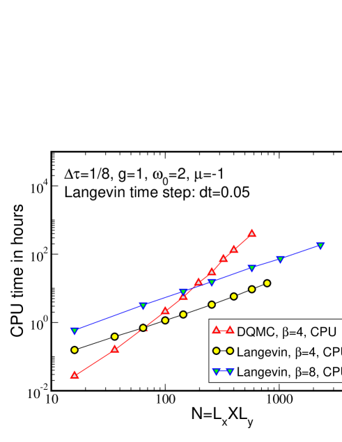
Figure 1: (Color online) CPU time versus system size in the Holstein limit ($\xi\to 0$) for DQMC and Langevin algorithms. DQMC scales as $N^{3}$ while Langevin scales essentially linearly for both values of $\beta$. $\lambda_{0}=g\sqrt{2\omega_{0}}$.

Figure 1 shows the of CPU time for the Langevin and DQMC algorithms as a function of system size $N=L_{x}\times L_{y}$ at phonon frequency $\omega_{0}=2$, electron phonon coupling $g=1$ and $\xi\to 0$ (i.e. the Holstein contact interaction limit). The chemical potential $\mu=-1$ is set so that the lattice is half-filled, $\rho=1$. For this figure, the same number of sweeps was chosen for all the DQMC sizes, and a different fixed number of sweeps for the Langevin runs. The goal is simply to show the scaling of CPU time.

The log-log plot demonstrates the expected $N^{3}$ scaling for DQMC, and a near-linear scaling for the Langevin approach. That the power is slightly larger than one is a consequence of a modest increase in the number of conjugate gradient iterations with $N$. The Langevin approach already becomes more efficient than DQMC for relatively small lattice sizes, $N\sim 8\times 8$ for $\beta=4$. A key feature of Fig. 1 is that the (near) linear scaling is no worse at $\beta=8$ than at $\beta=4$. In contrast, in simulations of the Hubbard model, the number of conjugate gradient iterations grows very rapidly at large $\beta$ and strong coupling $U$.

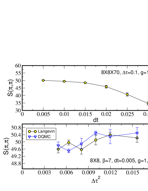
Figure 2: (Color online) Top: The dependence of $S(\pi,\pi)$ on the Langevin time step, ${\rm d}t$ in the ordered phase. For ${\rm d}t\leq 0.01$ the discretization error becomes linear in ${\rm d}t$. Bottom: The dependence of $S(\pi,\pi)$ on the imaginary time step, $\Delta\tau$, for both DQMC and Langevin. The Trotter-Suzuki errors are comparable in the two algorithms. ${\rm d}t=0.005$ used to integrate the Langevin equation gives excellent agreement with DQMC. The data are for the Holstein limit ($\xi\to 0$).

Figure 2 addresses the systematic errors in the Langevin approach. In the top panel, the charge density structure factor is shown as a function of Langevin step ${\rm d}t$. The lattice size is $N=8\times 8$ and the inverse temperature $\beta=7$ (deep in the ordered phase) with $\Delta\tau=0.1$. It is seen that for ${\rm d}t$ less than around $0.015$, the value of the structure factor changes very little and, in fact, the error varies linearly with ${\rm d}t$. For ${\rm d}t>0.015$, the error increases rapidly until the iterative process is destabilized beyond ${\rm d}t\approx 0.3$ for the parameters dshown in the figure. In the bottom panel the Trotter errors are assessed at fixed Langevin step ${\rm d}t=0.005$ and compared with those arising from DQMC. They are seen to be less than one percent up to $\Delta\tau^{2}=0.016$ ($\Delta\tau=0.125$), and are comparable for the two methods.

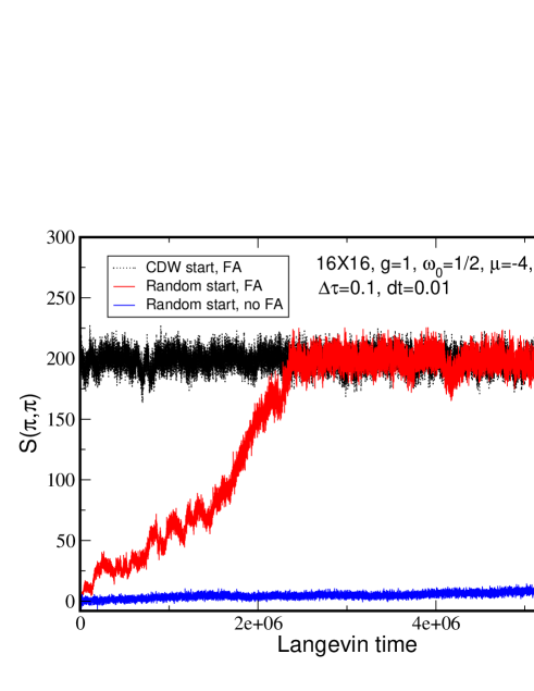
Figure 3: (Color online) $S(\pi,\pi)$ as a function of Langevin time, comparing Fourier acceleration (FA) with unaccelerated evolution. The red (FA) and blue (no FA) curves have the same random initial configuration of the phonon field. It is clear that for large systems FA is crucial for equilibration. The initial configuration for the black curve is CDW: The phonon field has an initial checkerboard configuration.

Equilibration and autocorrelation times play a key role in the assessment of any algorithm. Figure 3 shows the equilibration of the charge density structure factor $S(\pi,\pi)$ on a $N=16\times 16$ lattice at $\beta=7$ with $\omega_{0}=0.5$, $g=1$ ($\lambda_{0}=1)$ and $\xi\to 0$. The lattice is half-filled ($\mu=-4$). In the absence of Fourier Acceleration, and with a random start, the system remains in the disordered state ($S(\pi,\pi)$ small) even out to six million time steps. On the other hand, if FA is implemented, it grows steadily, achieving a value consistent with the known CDW order at $t\sim 2\times 10^{6}$. If the simulation is started in a CDW pattern, it remains in that phase.

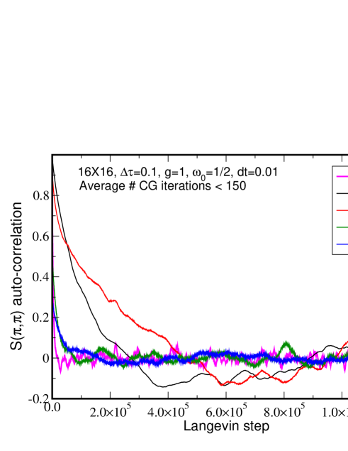
Figure 4: (Color online) The autocorrelation function of accelerated Langevin dynamics of the Holstein model for several $\beta$ values. The relaxation time is longest for $L_{\tau}=40,\,50$ ($\beta=4,\,5$) near the critical temperature, $\beta\approx 4.5$.

Figure 4 shows the autocorrelation function in the presence of FA for a $N=16\times 16$ lattice. Deep in the CDW phase, $L_{\tau}=60,70$ ($\beta=6,7$), as well as in the high temperature phase, $L_{\tau}=30$ ($\beta=3$) the autocorrelation time is relatively short. As is typical, autocorrelation times are long near the critical $\beta_{c}\sim 4.5$ as seen from the data with $L_{\tau}=40,50$ ($\beta=4,5$).

IV The Phase Diagram of the Long Range Model

We focus in this paper on a longer range el-ph coupling given by Eq. 1. Several initial efforts have been made to study this situationjohnston18 ; devereaux18 . They have found a significant tendency to phase separation. The qualitative physics behind this is clear: In the Holstein model an electron of one spin distorts the phonon on its same site, attracting an electron of opposite spin there. The Pauli principle precludes any further clustering. If, however, the interaction extends to neighboring sites, electrons will get attracted there. These, in turn will bring in yet more particles on next-near neighbor sites. This cascading effect costs kinetic energy, and entropy, but still might dominate the physics. It has proven difficult to expose the extent of phase separation in traditional DQMC algorithms, since the longer range interaction makes the update of the Green function more expensive. At minimum there is a succession of rank one updates whose number equals the number of sites within the interaction range. If $\xi$ is large enough, the expense goes from ${\cal O}(N^{3})$ to ${\cal O}(N^{4})$.

Our specific goal is to get the ground state phase diagram in the $\lambda_{0}-\xi$ plane. We begin by studying the real space density-density correlation function and its Fourier transform, the CDW structure factor, Eq.(20). In the disordered phase, $S(\pi,\pi)$ picks up contributions only from a small number of terms, while in the ordered phase, $S(\pi,\pi)$ will grow linearly with $N$.

Figure 5 shows $S(\pi,\pi)/N$ for several lattice sizes $N$ as a function of $\xi$ at fixed $\beta=9.6$, $\omega_{0}=0.5$ and $\lambda_{0}=1.5$. Data for different $N$ coincide at small $\xi$, indicating long range order. At $\xi\approx 0.4$, $S(\pi,\pi)$ falls rapidly. This parameter sweep represents one cut through the phase diagram of Fig. 11.

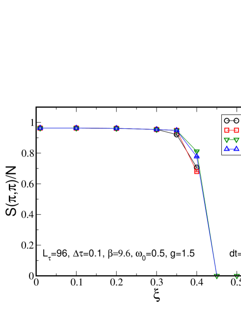
Figure 5: (Color online) The structure factor, $S(\pi,\pi)$ as a function of the range of the interaction, $\xi$, keeping the chemical potential tuned to half filling. When the interaction is large enough, $S(\pi,\pi)$ drops to zero due to phase separation. See the phase diagram of Fig. 11.

Figure 6, which shows the density for the same parameters as Fig. 5, suggests the collapse of CDW order is not due to the density-density correlator becoming random (as would occur if one heats the Holstein model above its $T_{c}$). Instead, the particle density plummets although the chemical potential is chosen to yield half filling. This suggests phase separation as $\xi$ grows.

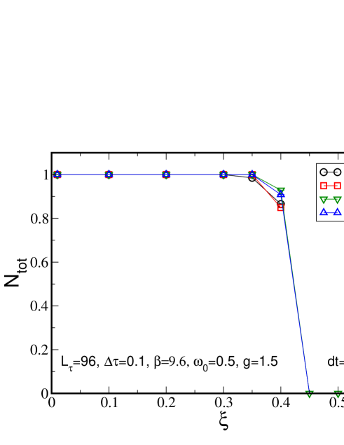
Figure 6: (Color online) Same as Fig. 5 but showing the total number of particles. For $\xi\gtrsim 0.4$ the occupation vanishes, indicating phase separation. See Fig. 11.

Figure 7 shows results in which instead $\lambda_{0}$ is increased at fixed $\xi=0.5$. Large density fluctuations set in at $\lambda_{0}\gtrsim 0.7$, again indicating phase separation. This provides another cut in the $\lambda_{0}$-$\xi$ plane to generate the phase boundary of Fig. 11.

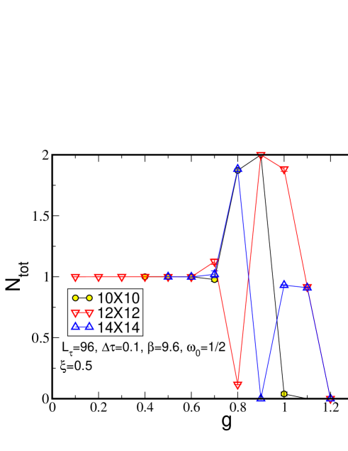
Figure 7: (Color online) The total occupation as a function of the interaction strength at fixed (large) $\xi$. For $\lambda_{0}>0.7$ the system is either empty or totally full, indicating phase separation. See Fig. 11.

Fixing $\xi=0.2$, $S(\pi,\pi)$ grows rapidly at $\lambda_{0}\sim 0.6$ for $\beta=9.6$ (Fig. 8). We believe that the region of small $S(\pi,\pi)$, $\lambda_{0}\lesssim 0.6$, is associated with the fact that the transition temperature is exponentially low. We see no evidence for phase separation. This is also confirmed in Fig. 9 where one sees a growth of $S(\pi,\pi)$ in the small $\lambda$ region as $T$ is lowered. The observation of ordered phases at weak coupling is often a subtle issue in finite temperature simulations, since, for example, one often has BCS-like functional forms $T_{c}\sim\omega e^{-ct/\lambda}$ which become exponentially small as $\lambda$ decreases. This is supported by the fact that $S(\pi,\pi)$ grows as $\beta$ increases, unlike situations where there is a disordered phase below a critical coupling value, as occurs on a honeycomb latticepaiva05 ; zhang18 . The finite temperature difficulty in observing the CDW phase was also noted in Ref. weber17, .

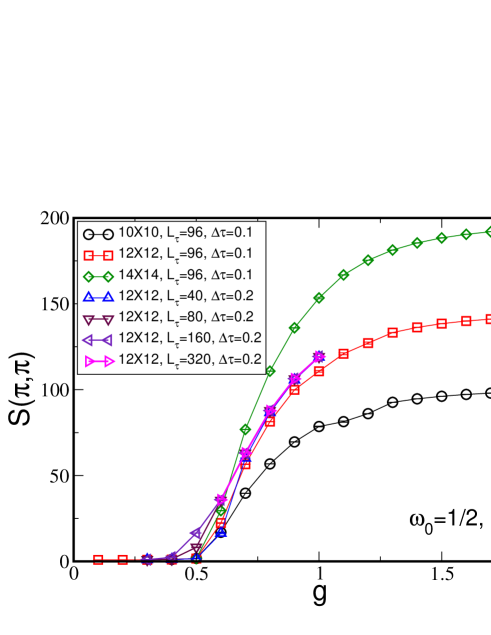
Figure 8: (Color online) $S(\pi,\pi)$ as a function of $\lambda_{0}$ at fixed $\xi=0.2$ where there is no phase separation (See Fig. 11). As $\lambda_{0}$ decreases, $S(\pi,\pi)$ decreases, becoming small for $\lambda_{0}<0.4$. We believe this is due to an exponentially small $T_{c}$ which has decreased below our simulation temperatures $T\sim(1/16-1/64)\,t$ rather than a lack of CDW order. See text.

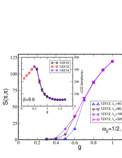
Figure 9: (Color online) Same as Fig. 8 but for one size and several values of $\beta$. $S(\pi,\pi)$ increases, and then saturates, as $\beta$ is increased. We are unable to see the CDW phase unambiguously for $\lambda_{0}<0.4$. Inset: For the same $\omega_{0}$ and $\xi$ and for $\beta=9.6$, we show the average number of CG iterations as a function of the coupling $g$. At weak coupling, the number of iterations is large, peaks at $g=0.5$, and decreases rapidly as the CDW gap strengthens. Note the absence of dependence on system size.

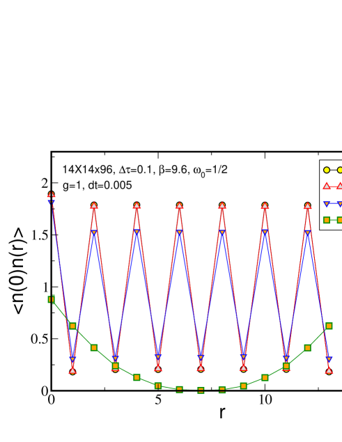
Figure 10: (Color online) The density correlation function as a function of distance at fixed $g=1$ and $\xi=0.1,\,0.2,\,0.3,\,0.4$. For the first three values of $\xi$, the system is in the CDW phase, as is clear from the robust oscillation of the correlation function. For $\xi=0.4$ the system has undergone phase separation.

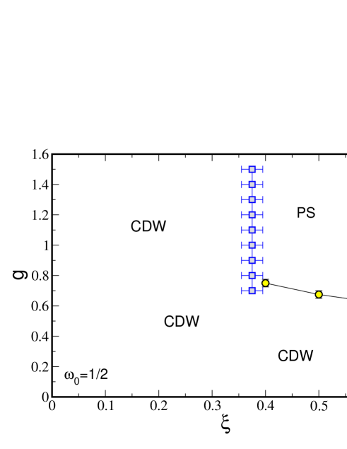
Figure 11: (Color online) The phase diagram in the $g$-$\xi$ plane at half-filling and constant $\beta=9.6$. The phonon frequency is fixed at $\omega=1/2$. At small $\xi$, the Holstein limit CDW correlations form. This occurs even at weak coupling owing to the Fermi surface nesting on the square lattice. As $\xi$ increases, phase separation occurs.

Although we have focused on the (momentum space) CDW structure factor, one can also of course observe the oscillating density correlations directly in real space. An example is given in Fig. 10. At fixed $\beta=9.6$ and $g=1.0$, robust density oscillations occur up to $\xi=0.3$. For $\xi=0.4$ the system has undergone phase separation and the density correlation function no longer exhibits CDW oscillations.

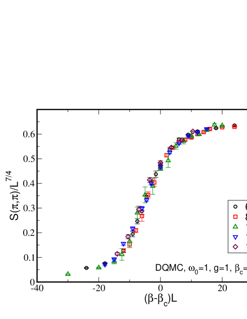
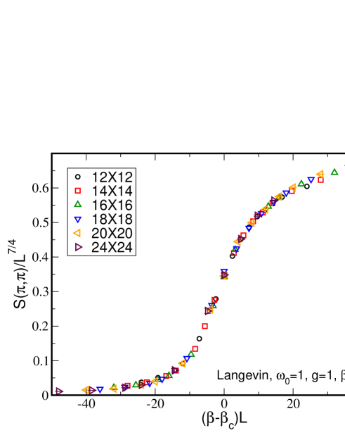
Figure 12: (Color online) Top: Scaling of the structure factor near the finite temperature transition from disordered to CDW phasecosta18 using DQMC. Bottom: Same but using Langevin. Note the larger system sizes and the cleaner collapse in the latter case. In the lower panel, the error bars are smaller than the symbols.

Taken together, Figs. 5-10 can be used to generate the phase diagram at $beta=9.6$ shown in Fig. 11. The small $\lambda$ regions are labeled as CDW based on the earlier arguments concerning the critical temperature.

Figure 11 shows the phase diagram at very low temperature. Since CDW formation breaks a discrete symmetry, we expect that in two dimensions the phase transition occurs at finite critical temperarture, $T_{c}$. Figure 12 shows a finite size scaling analysis of $S(\pi,\pi)$, making use of the expected Ising critical exponentsscalettar89 ; noack91 ; weber17 . The top panel uses data from the ‘traditional’ DQMC approach which is based on single phonon field updates and scales as ${\cal O}(N^{3})$, while the bottom panel shows the Langevin results with computation time scaling linearly with $N$. The ability to simulate larger lattice sizes is seen to provide a more convincing data collapse, which occurs as the thermodynamic limit is approached. In addition, the efficiency of the algorithm allows us to get more precise results in reasonable computation time. As a benchmark, we note that the simulations of the $12\times 12$ system took about four times longer with the Langevin algorithm than with DQMC, but the precision is much better than a factor of two. For larger systems sizes, the run time difference favors Langevin even more because of the linear scaling as opposed to cubic for DQMC. We performed such finite size scaling to find the critical inverse temparature, $\beta_{c}(\xi)$, as $\xi$ is increased. Figure 13 shows the resulting phase diagram in the ($\xi,\beta_{c}$) plane illustrating that as $\xi$ increases, $\beta_{c}$ increases rapidly until phase separation occurs at large enough $\xi_{c}\approx 0.55$. We did not determine $\beta_{c}$ beyond $\xi=0.3$ since it becomes very large.

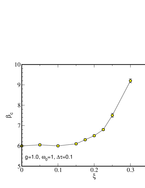
Figure 13: (Color online) The critical inverse temperature, $\beta_{c}$, as a function of the range of the electron-phonon interaction, $\xi$. $\beta_{c}$ was obtained by performing finite size scaling analysis as in Fig. 12.

V Conclusions and Outlook

In this paper we have formulated a Langevin-based Quantum Monte Carlo algorithm for an interacting electron-phonon Hamiltonian, augmented by Fourier Acceleration. Variation of the phonon field in the imaginary time direction is moderated by the phonon kinetic energy. As a consequence, the rapid growth in the number of conjugate gradient iterations needed in such approaches to the Hubbard model is not present here.

We have presented tests of our method which quantify various systematic errors. Comparisons with single update ${\cal O}(N^{3})$ simulations using DQMC show that the Langevin method gives physically correct results, and also indicate that the cross-over where it becomes more efficient occurs at lattice sizes $N\sim 10^{2}$.

We have applied the method to an electron-phonon model with finite range (i.e. momentum-dependent) interaction. This is a natural target, since single update algorithms scale as ${\cal O}(N^{4})$ and hence have proven extremely challenging. The phase diagram obtained indicates a strong tendency towards phase separation, even with correlation lengths as small as $\xi\sim 0.35$, a situation in which the near-neighbor coupling is nearly two orders of magnitude smaller than the on-site interaction.

This sensitivity to finite $\xi$ suggests that application of such models to materials with momentum-dependent $\tilde{\lambda}(q)$ will need to include some sort of electron-electron interaction to inhibit phase separation. This is a very challenging task owing to the resulting sign problem of doped systems which would lead to a complex Langevin. Such equations have been studied quite extensively in the context LGTaarts17 and recently applied to the one dimensional Hubbard modelloheac17 and ultra-cold fermionic atoms with unequal massesrammelmuller18 . The complex Langevin equation was also recently applied to the Holstein-Hubbard modelkarakuzu18 and shown to be very efficient in the parameter range $U>g^{2}/\omega_{0}$.

More direct applications of our approach will be to the on-site (Holstein) case, for which there is still an abundance of open questions, including studies of 3D and layered 2D systems, accurate determination of critical properties via finite size scaling, role of anharmonicities, and high resolution of observables in momentum space, all of which require large lattice sizes. In addition, SSH models where the hopping parameter fluctuates due to the nuclear oscillations can be treated efficiently with this algorithm. An interesting question to address is the competition between the contact Holstein coupling and the bond SSH coupling in determing the phase of the system.

VI Acknowledgements

The work of RTS was supported by DOE-SC0014671. GGB is supported by the French government, through the UCAJEDI Investments in the Future project managed by the National Research Agency (ANR) with the reference number ANR-15-IDEX-01. We thank Steven Johnston, WeiTing Chiu, and Thomas Devereaux for useful conversations.

References

- (1) “A New Algorithm for the Numerical Simulation of Fermions”, R.T. Scalettar, D.J. Scalapino, and R.L. Sugar, Phys. Rev. B34, 7911 (1986).
- (2) “A Hybrid-Molecular Dynamics Algorithm for the Numerical Simulation of Many Electron Systems”, R.T. Scalettar, D.J. Scalapino, R.L. Sugar, and D. Toussaint, Phys. Rev. B36, 8632 (1987).
- (3) “A High Quality Preconditioning Technique for Multi-Length-Scale Symmetric Positive Definite Linear Systems”, I. Yamazaki, Z. Bai, W. Chen, and R. Scalettar, Numerical Mathematics: Theory, Methods and Applications 2, 469 (2009).
- (4) “Numerical Methods for Quantum Monte Carlo Simulations of the Hubbard Model”, Zhaojun Bai, Wenbin Chen, Richard Scalettar and Ichitaro Yamazaki, in “Multi-Scale Phenomena in Complex Fluids” edited by Thomas Y. Hou, Chun Liu and Jian-Guo Liu, pp. 1-110, Higher Education Press (2009).
- (5) “Revisiting the hybrid quantum Monte Carlo method for Hubbard and electron-phonon models”, Stefan Beyl, Florian Goth, and Fakher F. Assaad Phys. Rev. B97, 085144 (2018).
- (6) “Continuous-Time Quantum Monte Carlo Algorithm for the Lattice Polaron”, P.E. Kornilovitch, Phys. Rev. Lett. 81, 5382 (1998).
- (7) “Ground-state dispersion and density of states from path-integral Monte Carlo: Application to the lattice polaron”, P.E. Kornilovitch, Phys. Rev. B60, 3237 (1999).
- (8) “Polaron dynamics and bipolaron condensation in cuprates”, A. S. Alexandrov, Phys. Rev. B61, 12315 (2000).
- (9) “Quantum Monte Carlo and variational approaches to the Holstein model”, M. Hohenadler, H. G. Evertz, and W. von der Linden, Phys. Rev. B69, 024301 (2004).
- (10) “Dimensionality effects on the Holstein polaron”, L.-C. Ku, S.A. Trugman, and J. Bonca, Phys. Rev. B65, 174306 (2002).
- (11) “Effect of electron-phonon interaction range on lattice polaron dynamics: A continuous-time quantum Monte Carlo study”, P.E. Spencer, J.H. Samson, P.E. Kornilovitch, and A.S. Alexandrov, Phys. Rev. B71, 184310 (2005).
- (12) “Two dimensional Hubbard-Holstein bipolaron”, A. Macridin, G.A. Sawatzky, and M. Jarrell, Phys. Rev. B69, 245111 (2004).
- (13) “Effects of dimensionality and anisotropy on the Holstein polaron”, A.H. Romero, D.W. Brown, and K. Lindenberg, Phys. Rev. B60, 14080 (1999).
- (14) “Holstein polaron”, J. Bonća, S.A. Trugman, and I. Batistić, Phys. Rev. B60, 1633 (1999).
- (15) “The extended vs standard Holstein model; results in two and three dimensions”, Carl J. Chandler, F. Marsiglio, Phys. Rev. B90, 125131 (2014).
- (16) “Bipolarons from long-range interactions: Singlet and triplet pairs in the screened Hubbard-Fröhlich model on the chain”, J.P. Hague and P.E. Kornilovitch, Phys. Rev. B80, 054301 (2009).
- (17) “Competition of Pairing and Peierls–CDW Correlations in a 2–D Electron–Phonon Model”, R.T. Scalettar, D.J. Scalapino, and N.E. Bickers, Phys. Rev. B40, 197 (1989).
- (18) “CDW and Pairing Susceptibilities in a Two Dimensional Electron–Phonon Model”, R.M. Noack, D.J. Scalapino, and R.T. Scalettar, Phys. Rev. Lett. 66, 778 (1991).
- (19) “Charge Density Wave Gap Formation in the 2–dimensional Holstein Model at Half–Filling”, P. Niyaz, J.E. Gubernatis, R.T. Scalettar, and C. Y. Fong, Phys. Rev. B48, 16011 (1993).
- (20) “Two-Dimensional Holstein Model: Critical Temperature, Ising Universality, and Bipolaron Liquid”, M. Weber and M. Hohenadler, arXiv:1709.01096.
- (21) “Phonon dispersion and the competition between pairing and charge order”, N.C. Costa, T. Blommel. W.-T. Chiu, G.G. Batrouni, and R.T. Scalettar, Phys. Rev. Lett. 120, 187003.
- (22) “Electrons in Lattice Fields”, H. Fröhlich, Adv. Phys. 3, 325 (1954).
- (23) “Studies of Polaron Motion 1. The Molecular-Crystal Model”, T. Holstein, Ann. Phys. N.Y. 8, 325 (1959).
- (24) “Momentum average approximation for models with electron-phonon coupling dependent on the phonon momentum”, G.L. Goodvin and M. Berciu, Phys. Rev. B78, 235120 (2008).
- (25) “Aspects of electron-phonon interactions with strong forward scattering in FeSe Thin Films on SrTiO 3 substrates”, Y. Wang, K. Nakatsukasa, L. Rademaker, T. Berlijn, and S. Johnston, arXiv:1602.00656.
- (26) “Strong polaronic behavior in a weak coupling superconductor”, A.G. Swartz, H. Inoue, T.A. Merz, Y. Hikita, S. Raghu, T.P. Devereaux, S. Johnston, and H.Y. Hwang, arXiv:1608.05621.
- (27) “Extended Phonon Collapse and the Origin of the Charge-Density Wave in 2H-NbSe”, F. Weber, S. Rosenkranz, J.-P. Castellan, R. Osborn, R. Hott, R. Heid, K.-P. Bohnen, T. Egami, A.H. Said, and D. Reznik, Phys. Rev. Lett. 107, 107403 (2011).
- (28) “Effect of Electron-Phonon Interaction Range for a Half-Filled Band in One Dimension”, M. Hohenadler, F.F. Assaad, and H. Fehske, Phys. Rev. Lett. 109, 116407 (2012).
- (29) “Directly characterizing the relative strength and momentum dependence of electron-phonon coupling using resonant inelastic x-ray scattering”, T.P. Devereaux, A.M. Shvaika, K. Wu, K. Wohlfeld, C.J. Jia, Y. Wang, B. Moritz, L. Chaix, W.-S. Lee, Z.-X. Shen, G. Ghiringhelli, and L. Braicovich, arXiv 1605.03129.
- (30) “Monte Carlo calculations of coupled boson-fermion systems. I”, R. Blankenbecler, D.J. Scalapino, and R.L. Sugar, Phys. Rev. D24, 2278 (1981).
- (31) “A Novel Technique for the Simulation of Interacting Fermion Systems”, S. Sorella, S. Baroni, R. Car, and M. Parinello, Europhys. Lett. 8, 663 (1989).
- (32) “Langevin Simulations of Lattice Field Theories”, G. G. Batrouni, G. R. Katz, A. S. Kronfeld, G. P. Lepage, B. Svetitsky et K. G. Wilson, Physical Review D32, 2736 (1985).
- (33) “Symmetry Enforced Self-Learning Monte Carlo Method Applied to the Holstein Model”, Chuang Chen, Xiao Yan Xu, Junwei Liu, George Batrouni, Richard Scalettar and Zi Yang Meng, Phys. Rev. B98, 041102 (2018), rapid communication.
- (34) S. Johnston, unpublished and private communication.
- (35) T.P. Devereaux, unpublished and private communication.
- (36) “Ground state and finite temperature signatures of quantum criticality in the Half-filled Hubbard Model on a Honeycomb Lattice”, Thereza Paiva, R.T. Scalettar, W. Zheng, R.R.P. Singh, and J. Oitmaa, Phys. Rev. B72, 085123 (2005).
- (37) Y.X. Zhang, W.T. Chiu, N.C. Costa, G.G. Batrouni, and R.T. Scalettar, unpublished.
- (38) G. Aarts, E. Seiler, D. Sexty, I.-O. Stamatescu, J. High Energ. Phys. 44 (2017).
- (39) C. Loheac, J. E. Drut, Phys. Rev. D95, 094502 (2017).
- (40) L. Rammelmüller, J. E. Drut, J. Braun, J. Phys.: Conf. Ser. 1041, 012006 (2018).
- (41) S. Karakuzu, K. Seki, and S. Sorella, arXiv:1808.07759.