Where do the AMS-02 anti-helium events come from?

Abstract

We discuss the origin of the anti-helium-3 and -4 events possibly detected by AMS-02. Using up-to-date semi-analytical tools, we show that spallation from primary hydrogen and helium nuclei onto the ISM predicts a $\overline{{}^{3}{\rm He}}$ flux typically one to two orders of magnitude below the sensitivity of AMS-02 after 5 years, and a $\overline{{}^{4}{\rm He}}$ flux roughly 5 orders of magnitude below the AMS-02 sensitivity. We argue that dark matter annihilations face similar difficulties in explaining this event. We then entertain the possibility that these events originate from anti-matter-dominated regions in the form of anti-clouds or anti-stars. In the case of anti-clouds, we show how the isotopic ratio of anti-helium nuclei might suggest that BBN has happened in an inhomogeneous manner, resulting in anti-regions with a anti-baryon-to-photon ratio $\mathrm{bar}{\eta}\simeq 10^{-3}\eta$. We discuss properties of these regions, as well as relevant constraints on the presence of anti-clouds in our Galaxy. We present constraints from the survival of anti-clouds in the Milky-Way and in the early Universe, as well as from CMB, gamma-ray and cosmic-ray observations. In particular, these require the anti-clouds to be almost free of normal matter. We also discuss an alternative where anti-domains are dominated by surviving anti-stars. We suggest that part of the unindentified sources in the 3FGL catalog can originate from anti-clouds or anti-stars. AMS-02 and GAPS data could further probe this scenario.

I Introduction

The origin of cosmic ray (CR) anti-matter is one of the many conundrums that AMS-02 is trying to solve thanks to precise measurements of CR fluxes at the Earth. In over six years, AMS-02 has accumulated several billion events, whose composition is mostly dominated by protons and helium nuclei. Moreover, positrons and antiprotons have been frequently observed and are the object of intense theoretical investigations in order to explain their spectral features. Indeed, anti-matter particles are believed to be mainly of secondary origin, i.e., they are created by primary CR nuclei (accelerated by supernova-driven shock waves) impinging onto the interstellar medium (ISM). However, deviations from these standard predictions have been observed, hinting at a possible primary component. In the case of positrons, a very significant high-energy excess has already been seen in PAMELA data Adriani et al. (2010). The main sources under investigation to explain this excess are DM and pulsars (see e.g. Bergstrom et al. (2008); Cirelli and Strumia (2008); Cirelli et al. (2009a); Nelson and Spitzer (2010); Arkani-Hamed et al. (2009); Harnik and Kribs (2009); Fox and Poppitz (2009); Pospelov and Ritz (2009); March-Russell and West (2009); Dienes et al. (2013); Kopp (2013); Yuksel et al. (2009); Profumo (2011); Kawanaka et al. (2010); Yuan et al. (2015); Yin et al. (2013); Hooper et al. (2009); Cholis et al. (2009a, b); Cholis and Hooper (2013); Boudaud et al. (2015a, 2017); Hooper et al. (2017); Cholis et al. (2018a, b)). In the case of antiprotons, a putative excess at the GeV-energy Cuoco et al. (2017) is under discussion Reinert and Winkler (2017). Still, antiprotons represent one of the most promising probes to look for the presence of DM in our Galaxy through its annihilation.

But the searches for anti-matter CR do not limit themselves to antiprotons and positrons. Hence, many theoretical and experimental efforts are devoted to detecting anti-deuterons, which are believed to be a very clean probe of DM annihilations especially at the lowest energies (below tens of GeV) Chardonnet et al. (1997); Donato et al. (2000); Duperray et al. (2005); von Doetinchem et al. (2016). Similarly, measurement of the anti-helium nuclei CR flux is a very promising probe of new physics, that has been suggested to look for DM annihilations Duperray et al. (2005); Carlson et al. (2014); Cirelli et al. (2014); Coogan and Profumo (2017) or other sources of primary CR, such as anti-matter stars or clouds Steigman (1976); Belotsky:1998kz; Bambi and Dolgov (2007). Strikingly, AMS-02 has recently reported the possible discovery of eight anti-helium events in the mass region from 0 to 10 GeV/c² with $Z=2$ and rigidity $<50$ GV Choutko (2018). Six of the events are compatible with being anti-helium-3 and two events with anti-helium-4. The total event rate is roughly one anti-helium in a hundred million heliums. This preliminary sample includes one event with a momentum of $32.6\pm 2.5$ GeV/c and a mass of $3.81\pm 0.29$ GeV/c² compatible with that of anti-helium-4. Earlier already, another event with a momentum of 40.3 $\pm$ 2.9 GeV and a mass compatible with anti-helium-3 had been reported Ting (2016).

In this paper, we discuss various possibilities for the origin of AMS-02 anti-helium events. Should these events be confirmed, their detection would be a breakthrough discovery, with immediate and considerable implications onto our current understanding of cosmology. The discovery of a single anti-helium-4 nucleus is challenging to explain in terms of known physics. In this article, we start stressing why such a discovery is unexpected. For this, we re-evaluate the secondary flux of anti-helium nuclei. In particular, we provide the first estimate of the $\overline{{}^{4}{\rm He}}$ flux at the Earth coming from the spallation of primary CR onto the ISM. We show that it is impossible to explain AMS results in terms of a pure secondary component, even though large uncertainties still affect the prediction. Moreover, we argue that the DM explanations of these events face similar difficulties, although given the virtually infinite freedom in the building of DM models, it is conceivable that a tuned scenario might succeed in explaining these events.

We then discuss the implications of the anti-helium observation. We essentially suggest that the putative detection of $\overline{{}^{3}{\rm He}}$ and $\overline{{}^{4}{\rm He}}$ by AMS-02 indicates the existence of an anti-world, i.e., a world made of anti-matter, in the form of anti-stars or anti-clouds. We discuss properties of these regions, as well as relevant constraints on the presence of anti-clouds in our Galaxy. We present constraints from the survival of anti-clouds in the Milky-Way and in the early Universe, as well as from CMB, gamma-ray and cosmic-ray observations. We show in particular that these require the anti-clouds to be almost free of normal matter. Moreover, we show how the isotopic ratio of anti-helium nuclei might suggest that BBN happened inhomogeneously, resulting in anti-regions with a anti-baryon-to-photon ratio $\mathrm{bar}{\eta}\simeq 10^{-3}\,\eta$. Given the very strong constraints applying to the existence and survival of anti-clouds, we also discuss an alternative scenario in which anti-domains are dominated by anti-stars. We suggest that part of the unidentified sources in the 3FGL catalog can be anti-clouds or anti-stars. Future AMS-02 and GAPS data could further probe this scenario.

The paper is structured as follows. Section II is devoted to a thorough re-evaluation of the secondary astrophysical component from spallation within the coalescence scheme. A discussion on the possible limitations of our estimates and on the DM scenario is also provided. In section III, we discuss the possibility of anti-domains in our Galaxy being responsible for AMS-02 events. Properties of anti-clouds and their constraints are presented in sec III.1, while the alternative anti-star scenario is developed in section III.2. Finally, we draw our conclusions in sec. IV.

II Updated calculation of $\mathrm{bar}{d}$, $\overline{{}^{3}{\rm He}}$ and $\overline{{}^{4}{\rm He}}$ from spallation onto the ISM

As for any secondaries, the prediction of the $\overline{{}^{3}{\rm He}}$ flux at Earth is the result of two main processes affected by potentially large uncertainties: i) the production due to spallation of primary CR onto the ISM and ii) the propagation of cosmic rays in the magnetic field of our Galaxy, eventually modulated by the impact of the Sun. In this section, we briefly review how to calculate the secondary flux of $\overline{{}^{3}{\rm He}}$ from spallation onto the ISM in a semi-analytical way.

II.1 Source term for anti-nuclei in the coalescence scenario

The spallation production cross-section of an anti-nucleus A from the collision of a primary CR species $i$ onto an ISM species $j$ can be computed within the coalescence scenario as follows:

$$\frac{E_{A}}{\sigma_{ij}}\frac{d^{3}\sigma^{ij}_{A}}{d^{3}k_{A}}=B_{A}\cdot\bigg{(}\frac{E_{p}}{\sigma_{ij}}\frac{d^{3}\sigma^{ij}_{p}}{d^{3}k_{p}}\bigg{)}^{\!Z}\cdot\bigg{(}\frac{E_{n}}{\sigma_{ij}}\frac{d^{3}\sigma^{ij}_{n}}{d^{3}k_{n}}\bigg{)}^{\!A-Z}\,,$$ (1)

where $\sigma^{ij}$ is the total inelastic cross section for the $ij$ collision, and the constituent momenta are taken at $k_{p}=k_{n}=k_{A}/A$. $B_{A}$ is the coalescence factor, whose role is to capture the probability for A anti-nucleons produced in a collision to merge into a composite anti-nucleus. It is often written as

$$B_{A}=\bigg{(}\frac{4\pi}{3}\frac{p_{\rm coal}^{3}}{8}\bigg{)}^{\!A-1}\frac{m_{A}}{m_{p}^{Z}m_{n}^{A-Z}}\,,$$ (2)

where $p_{\rm coal}$ is the diameter of a sphere in phase-space within which anti-nucleons have to lie in order to form an anti-nucleus. The coalescence factor $B_{A}$ is a key quantity which can be estimated from $pp$-collision data, as has been done recently by the ALICE collaboration Acharya et al. (2017) for anti-deuteron and anti-helium. We use the values measured at low transverse momentum as these are adequate for CR spallation, namely $B_{2}\simeq(15\pm 5)\times 10^{-2}$ GeV² and $B_{3}\simeq(2\pm 1)\times 10^{-4}$ GeV⁴. We extrapolate these values to $pA$ and $AA$ collisions. There is no measurement of $B_{4}$ yet available. Hence, we make use of eq. 2 in order to extract the coalescence momentum (common to each species in the coalescence model) from the $B_{3}$ measurement. This gives a coalesence momentum that varies between $0.218$ GeV and $0.262$ GeV. Using the measurement of $B_{2}$, the coalescence momentum varies between $0.208$ GeV and $0.262$ GeV, which is in excellent agreement with the value extracted from $B_{3}$. We stress that the fact that the coalescence momenta extracted from both coalescence factors agree is far from trival. It indicates that the coalescence scenario is much more predictive and accurate than one might have naively expected from its apparent simplicity. To phrase this otherwise: from the $B_{2}$ measurement of ALICE, one can predict how many anti-helium-3 ALICE should measure; this turns out to be in very good agreement with the actual measurement, which is quite remarkable. The final step is thus to apply eq. 2 to the case of anti-helium-4. We find that $B_{4}$ varies between $7.7\times 10^{-7}$ GeV⁶ and $3.9\times 10^{-6}$ GeV⁶.

In the context of antiproton production, it has been found that di Mauro et al. (2014)

$$E_{n}\frac{d^{3}\sigma^{ij}_{n}}{d^{3}k_{n}}=\Delta_{np}\,E_{p}\frac{d^{3}\sigma^{ij}_{p}}{d^{3}k_{p}}\,,$$ (3)

where $\Delta_{np}\simeq 1.3$ is introduced to model the isospin symmetry breaking. However, the ALICE experiment has extracted $B_{2}$ and $B_{3}$ assuming a perfect isospin symmetry between the antineutron and antiproton production. Hence, it would be wrong to make use of the factor $1.3$ in this context and we set $\Delta_{np}=1$. Additionally, we follow ref. Chardonnet et al. (1997) and compute the anti-deuterium production cross-section by evaluating the production cross-sections of the two anti-nucleons at respectively $\sqrt{s}$ and $\sqrt{s}-2E^{*}_{p}$ where $E^{*}_{p}$ denotes the anti-nucleon energy in the center of mass frame of the collision.

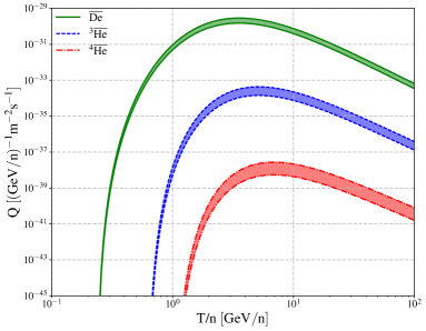
Figure 1: Local source term for the secondary production of $\mathrm{bar}{d}$, $\overline{{}^{3}{\rm He}}$ and $\overline{{}^{4}{\rm He}}$. The width of the prediction represents the uncertainty on the coalescence parameter $B_{A}$.

Similarly, for the anti-helium-3 and -4 we evaluate cross-sections decreasing the available center of mass energy $\sqrt{s}$ by $2E^{*}_{p}$ for each subsequent produced anti-nucleon. This ansatz has the merit of imposing energy conservation, although others are possible (see the discussion in Ref. Chardonnet et al. (1997)). We checked that adopting the other prescription $\sqrt{s}-m_{p}-E_{p}$ ̵̄suggested in Ref. Chardonnet et al. (1997) does not affect our conclusions. Another possibility to extend the coalescence analysis down to near-threshold collision energies is to introduce an interpolating factor $R$ in the RHS of eq. (1) as suggested, e.g., in Duperray et al. (2003); Blum et al. (2017). The secondary source term can then be readily computed as:

$$Q_{\rm sec}^{ij}(E_{A})=4\pi n_{j}\int_{E_{\rm th}}^{\infty}dE_{i}\,\phi_{i}(E_{i})\,\frac{d\sigma^{ij}_{A}}{dE_{A}}(E_{i},E_{A})\,,$$ (4)

with

$$\frac{d\sigma^{ij}_{A}}{dE_{A}}=2\pi k_{A}\int_{-1}^{1}\bigg{\{}E_{A}\,\frac{d^{3}\sigma^{ij}_{A}}{d^{3}k_{A}}\bigg{\}}d(-cos\theta)\,.$$ (5)

We assume the density of target hydrogen and helium in the ISM $n_{j}$ to be $0.9$ g/cm³ and $0.1$ g/cm³ respectively and make use of the demodulated flux of hydrogen and helium from AMS-02 with Fisk potential $730$ MV. To calculate the contribution of the main channel $p+p\to\mathrm{bar}{A}+X$, we make use of the recent $p+p\to\mathrm{bar}{p}+X$ cross-section parameterization from ref. di Mauro et al. (2014). In order to incorporate other production channels (i.e. from spallation of and onto ⁴He), we make use of scaling relations derived in ref. Norbury and Townsend (2007) and multiply the $p+p\to\mathrm{bar}{p}+X$ cross section by $(A_{T}A_{P})^{2.2/3}$ where $A_{P}$ and $A_{T}$ are the nucleon numbers of the projectile and target nuclei. The result of our computation is plotted in Fig. 1. A nice feature of the coalescence scenario is that it naturally predicts, for simple kinematic reasons, a hierarchical relation between the flux of $\overline{p}$, $\overline{d}$, $\overline{{}^{3}{\rm He}}$ and $\overline{{}^{4}{\rm He}}$, where each subsequent nucleus gets suppressed by a factor $10^{-4}-10^{-3}$.

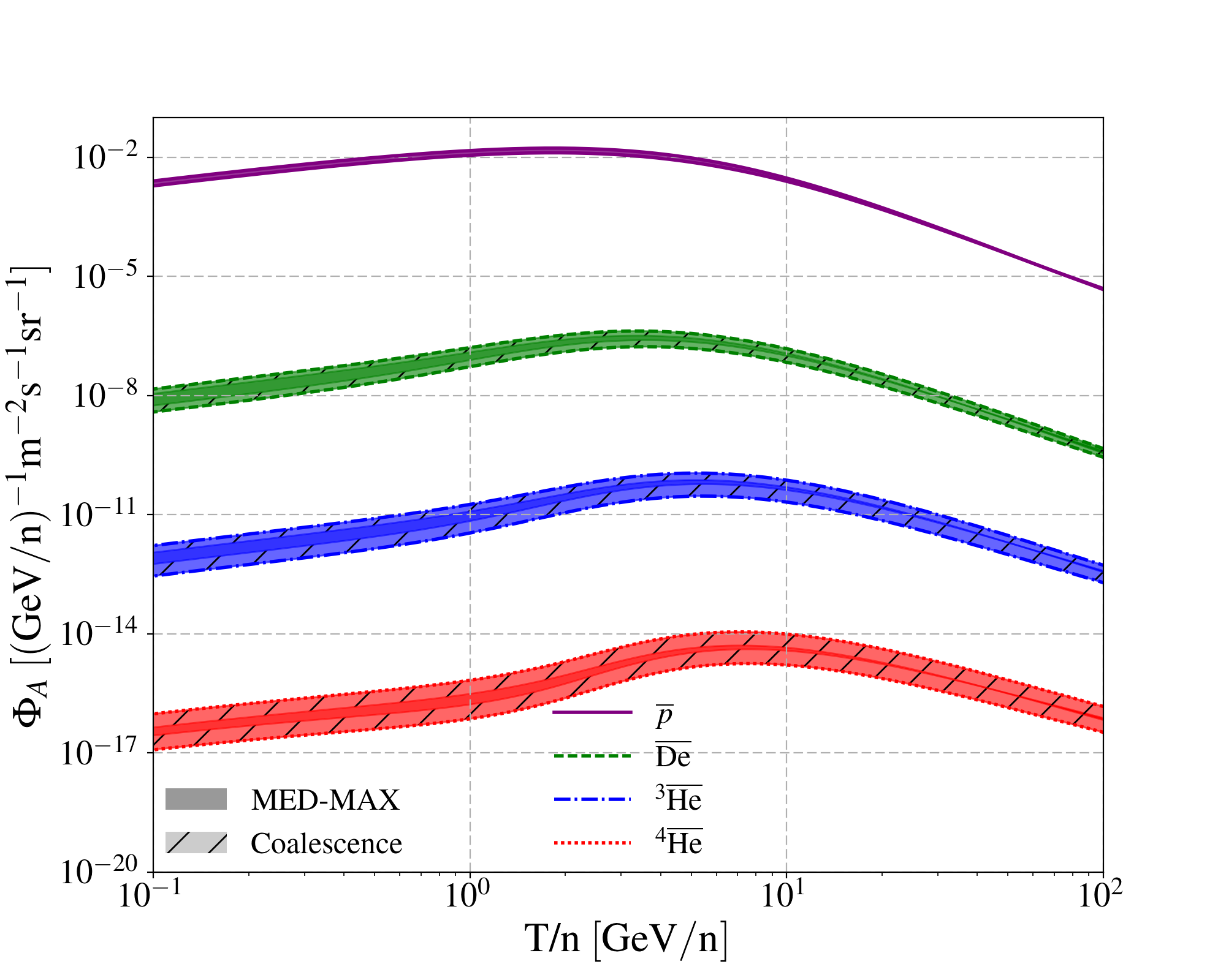
Figure 2: Predicted secondary flux of $\mathrm{bar}{p}$, $\mathrm{bar}{d}$, $\overline{{}^{3}{\rm He}}$ and $\overline{{}^{4}{\rm He}}$ showing the uncertainty associated to the propagation and the coalescence momentum.

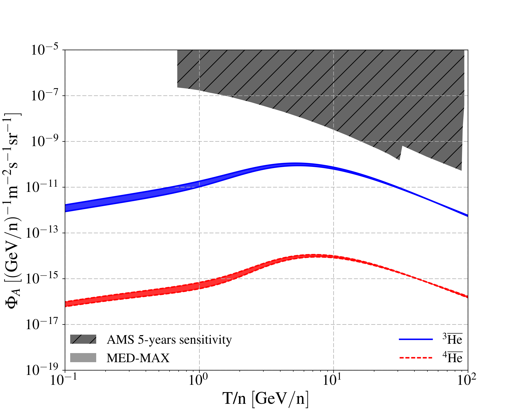
Figure 3: Predicted secondary flux of ${}^{3}\overline{\rm He}$ and ${}^{4}\overline{\rm He}$ using the upper limit on the coalescence momentum deduced from the ALICE experiment and showing the uncertainty associated to the MED to MAX propagation model from Ref. Donato et al. (2004). We also show the expected sensitivity from AMS-02 Kounine (2011).

II.2 Propagation in the Galaxy

To deal with propagation, we adapt the code developed in Refs. Boudaud et al. (2015b); Giesen et al. (2015). We model the Galaxy as a thin disk embedded in a 2D cylindrical (turbulent) magnetic halo and solve semi-analytically the full transport equation for a charged particle. We include all relevant effects, namely diffusion, diffusive reacceleration, convection, energy losses, $\overline{\rm A}$ annihilation and tertiary production. The equation governing the evolution of the energy and spatial distribution function $f$ of any species reads

$$\partial_{t}f+\partial_{E}\{b(E,\vec{x})f-K_{EE}(E)\partial_{E}f\}+\partial_{z}\{{\rm sign}(z)fV_{c}\}$$ (6)

$$-K(E)\nabla^{2}f=Q_{\rm II}+Q_{\rm III}-2h\delta(z)\Gamma_{\rm ann}f\,.$$

We choose a homogeneous and isotropic diffusion coefficient $K(E)=\beta K_{0}(R(E)/{\rm 1GV})^{\delta}$ where $\beta$ is the velocity of the particle and $R=p/(Ze)$ its rigidity, the ratio between the momentum $p=\sqrt{E^{2}-m_{A}^{2}}$ and electric charge $Ze$. The diffusive reacceleration coefficient is expressed as $K_{EE}(E)=(2v_{a}^{2}E^{2}\beta^{4})/(9K(E))$ where $v_{a}$ is the drift - or Alfvèn - velocity of the diffusion centers. The (subdominant) energy losses are taken only in the disk $b(e,\vec{x})=2h\delta(z)b(E)$ where $h=100~{}$pc is the half-height of the disk and include ionization, Coulomb and adiabatic losses. The gradient of $V_{c}$ represents the convective wind, pushing outwards CR nuclei with respect to the disk. Possible annihilations of anti-nuclei $A$ in the disk are encoded in the last term on the RHS of eq. 6. The annilation rate takes the form $\Gamma_{\rm ann}=(n_{\rm H}+4^{2.2/3}n_{\rm He})v\sigma_{\rm ann}$, where $\sigma_{\rm ann}$ is the inelastic annihilation cross-section. To estimate the deuteron annihilation cross-section, we make use of the parameterization of the total cross-section of $\overline{\rm H}d$ from Ref. Hikasa et al. (1992) from which we remove the non-annihilating contribution using a measurement presented in Ref. Duperray et al. (2005), that is $\sigma_{\rm no-ann}^{\mathrm{bar}{d}{\rm H}}=4$ mb. This non-annihilation contribution is also used to calculate the tertiary source term $Q_{\rm III}$ following Ref. Boudaud et al. (2015b). Our prescription for annihilation and tertiary is in very good agreement with that presented in Ref. Duperray et al. (2005). To calculate the annihilation and tertiary production of anti-helium-3 and 4, we re-scale all cross-sections by a factor $(A/2)^{2.2/3}$. We treat the solar modulation in the force field approximation, setting the Fisk potential to 0.730 GV, the average value over AMS02 data taking period Ghelfi et al. (2017). Our secondary predictions of anti-deuteron, anti-helium-3 and -4 fluxes $\phi=\beta cf/(4\pi)$ are plotted in Fig. 2. We also show the antiproton flux associated to the same cross-section and propagation parameters, in order to illustrate the relative amount of each anti-species from secondary production in our Galaxy. However, we stress that our secondary prediction for antiproton is not the most up-to-date one and can be within 50% of the most recent calculation done in Ref. Reinert and Winkler (2017). We thus implemented the antiproton cross-section parameterization from Ref. Reinert and Winkler (2017) and checked that it does not affect our conclusions regarding anti-deuteron and anti-helium. We also checked that the impact of a break in the diffusion coefficient, as advocated in Ref. Génolini et al. (2017); Reinert and Winkler (2017) from an analysis of the recent AMS-02 proton, helium and B/C data, is negligible in the energy range we are interested in. Similarly, changing the value of the Fisk potential does not affect our prediction above a few GeV per nucleon.

In Fig. 3 we show the secondary prediction on anti-helium-3 and -4 compared to the advocated sensitivity of AMS-02 after 5 years Kounine (2011). In principle, we should compare our prediction to the measured flux, but this one is not available. Still, we can deduce from the claimed ratio of $\overline{\rm He}/{\rm He}\sim 10^{-8}$ that this flux is larger by a factor of $\sim 10$ than the advocated sensitivity of AMS-02 after 5 years around 10 GeV. Hence, we confirm that it is very challenging to explain the potential AMS02 anti-He signal as a pure secondary component. The $\overline{{}^{3}{\rm He}}$ is typically one to two orders of magnitude below the sensitivity of AMS-02 after 5 years, and the $\overline{{}^{4}{\rm He}}$ is roughly 5 orders of magnitude below AMS-02 sensitivity. Our results are in very good agreement with Ref. Korsmeier et al. (2017), who also found that the secondary prediction is, at best, roughly an order of magnitude below the tentative detection. Ref. Blum et al. (2017) on the other hand, concluded that a pure secondary explanation of the $\overline{{}^{3}{\rm He}}$ events was still viable. The main difference with Ref. Blum et al. (2017) lies in the range of values considered for the coalescence momentum. As the analysis of Ref. Blum et al. (2017) was completed, the Alice experiment had not yet published updated values for the coalescence factor of anti-helium $B_{3}$. Hence, the considered uncertainty range considered by Ref. Blum et al. (2017) is much broader (up to $20\times 10^{-4}$ GeV⁴) than the one considered in this work. When considering similar values of $B_{3}$, our results are in good agreement, even though the propagation of cosmic rays is treated in very different manners.

II.3 Boosting the production by spallation

Given the uncertainty on the mass measurement, it is conceivable that all of the anti-helium nuclei are actually $\overline{{}^{3}{\rm He}}$ isotopes. The standard $\overline{{}^{3}{\rm He}}$ calculation yields a flux that is a factor $\sim 30-100$ below what is measured by AMS-02. While uncertainties in the propagation are unlikely to be responsible for such mismatch, one might argue that the production term from spallation is underestimated. In order to boost the secondary flux, one needs to increase the coalescence factor $B_{3}$ by the same amount. The ALICE experiment has reported a measurement of the coalescence factor from $pp$-collision with center of mass energies of $0.9$ to $7$ TeV instead of the few hundreds of GeV at which collisions occur in the ISM. It is conceivable that the $B_{3}$ factor differs at lower energies. However, there are several arguments going against a large increase of the coalescence factor at low energy:

1. To commence, within the range of energies considered by ALICE (which spans an order of magnitude), the coalescence factor is very close to constant.

2. Then, there exist measurements Lemaire et al. (1979) of the $B_{2}$ and $B_{3}$ factors from heavy ion collisions with beam energies between 0.4 and 2.1 GeV/nuc. Albeit probed at a much lower center-of-mass energy than in the case of ALICE, the coalescence momentum is found to lie in the range 0.173–0.304 GeV for deuterium and 0.130–0.187 GeV for tritium and helium-3. In the latter case, $p_{\rm coal}$ is smaller than what is found by ALICE at LHC energies. Our prediction for the production of $\overline{{}^{3}{\rm He}}$ in primary CR collisions onto the ISM tends to overestimate the actual rate.

3. Finally, from a theoretical perspective, we expect the rate of coalescence of nucleons to be higher at high energy than at low energy. Indeed, the collision of a high energy particle (having a large Lorentz boost) will create a jet of particles whose opening angle is smaller than that of a low-energy collision. This in turn will increase the correlation of nucleons within the shower and thus the probability for nucleons to merge. Moreover, the production of many nucleons in low-energy collisions is strongly suppressed by the phase-space. This theoretical consideration is in good agreement with what has been found in recent Monte-Carlo simulation studies Gomez-Coral et al. (2018). The coalescence momentum (and hence the coalescence factor) decreases with lower center of mass energy. Hence, using the value obtained from ALICE data leads to a conversative over-estimation of the anti-nuclei secondary fluxes.

Alternatively, increasing the grammage seen by primary CRs along their journey towards Earth would enhance the yields of secondary nuclei. However such a scenario would result in all secondaries being affected in a similar way. Given the very good agreement (at the $\sim 20\%$ level) between the measurement of the $\mathrm{bar}{p}$ flux and its current best secondary estimate, a large increase in the grammage of our Galaxy is not realistic.

In conclusion, it seems to us extremely unlikely that a boosted production by spallation is responsible for such a large $\overline{{}^{3}{\rm He}}$ flux. Naturally, the presence of $\overline{{}^{4}{\rm He}}$ goes as well against this scenario.

II.4 A word on $\overline{{}^{3}{\rm He}}$ and $\overline{{}^{4}{\rm He}}$ from Dark Matter annihilation

A recent reanalysis of the $\overline{{}^{3}{\rm He}}$ yield from Galactic DM annihilation has been presented in Refs. Coogan and Profumo (2017); Korsmeier et al. (2017). The formalism is very similar to that of production by spallation, and the estimate of the DM source term depends as well on the knowledge of the coalescence momentum $p_{A}$ previously introduced. Similarly to secondary production, one expects a hierarchical relation between the fluxes of $\mathrm{bar}{p}$, $\mathrm{bar}{d}$, $\overline{{}^{3}{\rm He}}$ and $\overline{{}^{4}{\rm He}}$. According to Refs. Coogan and Profumo (2017); Korsmeier et al. (2017), if DM is responsible for AMS-02 events, it seems unlikely to observe $\overline{{}^{3}{\rm He}}$ without seeing a single $\overline{d}$ or overshooting $\overline{p}$ data. One caveat to this argument is that the sensitivity of AMS-02 to $\overline{d}$ might be (much) smaller than that to $\overline{{}^{3}{\rm He}}$ in some energy range Kounine (2011). Still, the possible presence of $\overline{{}^{4}{\rm He}}$ events is at odds with the DM scenario.

III $\overline{{}^{3}{\rm He}}$ and $\overline{{}^{4}{\rm He}}$ as an indication for an anti-world

Motivated by the $\overline{{}^{3}{\rm He}}$ and $\overline{{}^{4}{\rm He}}$, in this section we discuss the possibility that extended regions made of anti-matter have survived in our Galactic environment. There are many scenarios discussed in the literature and we present a few possibilities in sec. IV. The two possible cases that regions of anti-matter are present in our Galactic environment, are i) as ambient anti-matter mixed with regular matter in the ISM or in the form of anti-clouds; ii) in the form of anti-stars. The presence of $\overline{{}^{4}{\rm He}}$, if confirmed, would be a hint at the presence of such anti-regions. However, the fact that AMS-02 measures more $\overline{{}^{3}{\rm He}}$ than $\overline{{}^{4}{\rm He}}$ (roughly 3:1) is also interesting. As we discuss below, the isotopic ratio of anti-helium can potentially carry information about the physical conditions (in particular anti-matter and matter densities) within these regions.

III.1 Anti-clouds

We argue that the presence of clouds of anti-matter in our local environment can be responsible for the AMS-02 events. We discuss properties of these clouds and constraints that apply to this scenario (in particular from non-observation of $\gamma$-rays from matter-anti-matter annihilation).

III.1.1 Exotic BBN as an explanation of the anti-helium isotopic ratio

Standard big-bang nucleosynthesis (BBN) predicts the presence of many more ⁴He events, compared to ³He. For normal matter, the isotopic ratio of ⁴He:³He is roughly $10^{4}$:$1$. Within CRs, the isotopic ratio is higher since ³He can be produced through spallation of ⁴He and, according to PAMELA Adriani et al. (2016), it reaches $\sim$ 5:1 at a few GeV/n. Still, this is much lower than the possible measurement from AMS-02. As we have argued previously, increasing spallation by an order of magnitude is not realistic as it would affect all secondary species equally and lead to an over-prediction of $\mathrm{bar}{p}$s. Hence, inverting the isotopic ratio requires the presence of anisotropic BBN in regions where the (anti)-baryon-to-photon ratio strongly differs from that measured by Planck Ade et al. (2016). We therefore re-calculated the BBN yields for a large number of $\eta$ values using the BBN-code AlterBBN Arbey (2012) assuming CP-invariance for simplicity (Similar results are obtained with the BBN public code PRIMAT Pitrou et al. (2018)). We show in fig. 4 the number density of $\overline{\rm H}$, $\overline{\rm D}$ and $\overline{{}^{4}{\rm He}}$ normalized to $\overline{{}^{3}{\rm He}}$ as a function of the (anti-)baryon-to-photon ratio $\mathrm{bar}{\eta}$. The width of the band features the nuclear rate uncertainties . It is possible then to obtain the right isotopic ratio (i.e. roughly $\overline{{}^{4}{\rm He}}:\overline{{}^{3}{\rm He}}$ of 1:3) for $\mathrm{bar}{\eta}\simeq 1.3\!-\!6\times 10^{-13}$. Interestingly, this also predicts the presence of non-negligible CR $\mathrm{bar}{p}$ and $\mathrm{bar}{d}$ fluxes that we comment on in sec. III.1.6. We also point out that while $\eta$ from Planck refers to an average over the whole observable Universe, $\mathrm{bar}{\eta}$ is based on the isotopic ratio of $\overline{{}^{4}{\rm He}}:\overline{{}^{3}{\rm He}}$ and is therefore a local quantity. Depending on the object from which anti-helium events are originating, it is conceivable that this number varies from place to place even within our Galaxy such that on average the isotopic ratio of $\overline{{}^{4}{\rm He}}:\overline{{}^{3}{\rm He}}$ is as measured.

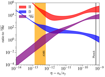
Figure 4: Abundance of $\overline{\rm H}$, $\overline{\rm D}$ and $\overline{{}^{4}{\rm He}}$ with respect to that of $\overline{{}^{3}{\rm He}}$ as a function of the (anti-)baryon-to-photon ratio $\mathrm{bar}{\eta}$. The Planck value is represented by the grey band. The value required by the AMS-02 experiment is shown by the orange band.

III.1.2 Some properties of the anti-domains

We can get some information about the anti-cloud regions from the ratio $\phi_{\overline{\rm He}}/\phi_{\rm He}$ (integrated over all energies), assuming that it reflects the ratio of the abundance of $\overline{\rm He}$ to ${\rm He}$ in the ISM (i.e. acceleration and propagation of CR are identical for matter and anti-matter), $N_{\overline{\rm He}}/N_{\rm He}$,

$$\frac{\phi_{\overline{\rm He}}}{\phi_{\rm He}}\simeq\frac{N_{\overline{\rm He}}}{N_{\rm He}}\simeq\bigg{(}\frac{n_{\overline{\rm He}}}{n_{\mathrm{bar}{p}}}\bigg{)}\bigg{(}\frac{n_{p}}{n_{\rm He}}\bigg{)}\bigg{(}\frac{n_{\overline{b}}}{n_{b}}\bigg{)}\bigg{(}\frac{V_{\overline{\rm M}}}{V_{\rm M}}\bigg{)}\,,$$ (7)

where $V_{\overline{\rm M}}$ and $V_{\rm M}$ represent the total volume of the anti-matter and matter regions in our Galaxy. We have assumed here that $n_{b}=n_{p}$ which is correct at the 10$\%$ level and that $n_{\overline{b}}=n_{\mathrm{bar}{p}}$ that, as shown in Fig. 4 is also correct at better than the 10$\%$ level. The CR data can also tell us about some of these ratios: i) $\phi_{\overline{\rm He}}/\phi_{\rm He}$ is of order $\sim 10^{-8}$; ii) the ratio $n_{p}/n_{\rm He}$ is of order $\sim$10; iii) the ratio $n_{\overline{\rm He}}/n_{\overline{p}}$, from the BBN calculation motivated by the isotopic ratio ${}^{4}\overline{\rm He}$:${}^{3}\overline{\rm He}$, is of order $\sim 10^{-5.5}\!-\!10^{-4}$. Hence we can get a constraint on the product of the total volume and density of these regions:

$$\bigg{(}\frac{n_{\overline{b}}}{n_{b}}\bigg{)}\bigg{(}\frac{V_{\overline{\rm M}}}{V_{\rm M}}\bigg{)}\sim 10^{-5}\!-\!10^{-3.5}\,.$$ (8)

It is possible to go one step further since the typical density of matter in the ISM is $n_{b}=1$ cm^-3 and $V_{\rm M}=2h\pi R_{\rm gal}^{2}\sim 6\times 10^{10}$ pc³. Moreover, if we assume that anti-matter forms spherical anti-clouds of radius $r_{\overline{\rm{c}}}$, we get $V_{\overline{\rm M}}=N_{\overline{\rm{c}}}(4\pi/3r_{\overline{\rm{c}}}^{3})$ and derive

$$n_{\overline{b}}\simeq 10^{5}-10^{6.5}N_{\overline{\mathrm{c}}}^{-1}\bigg{(}\frac{n_{b}}{1~{}\mathrm{cm}^{-3}}\bigg{)}\bigg{(}\frac{r_{\overline{c}}}{1~{}{\rm pc}}\bigg{)}^{-3}\mathrm{cm}^{-3}\,.$$ (9)

This key relation mostly relies on AMS-02 data and knowledge about Galactic properties. The only theoretical assumption so far is that the isotopic ratio of anti-helium is derived from BBN. From this we have additionally derived that at the time of BBN, $\mathrm{bar}{\eta}/\eta=n_{\mathrm{bar}{b}}/n_{b}\sim 10^{-3.5}-10^{-3}$. If this ratio still holds today, it would imply that there are $N_{\overline{\rm{c}}}\sim 10^{8}-10^{10}(r_{\overline{c}}/1{\rm pc})^{-3}$ anti-clouds in our Galaxy. The higher end of $N_{\overline{\mathrm{c}}}$ is close to the situation where the anti-clouds are connected in the ISM. However, this probably strongly overestimates the number of such objects, as cosmological evolution can affect these regions (and in particular the ratio $n_{\mathrm{bar}{b}}/n_{b}$) compared to primordial conditions. More realistically, AMS measured events would originate from a few highly-dense clouds.

III.1.3 Survival time of anti-matter in the Milky Way and the early Universe

We can gain information about the properties of the anti-matter regions and in particular constrain the amount of normal matter within them by estimating the typical lifetime of anti-matter in our Galaxy. The lifetime depends on the relative velocity between matter and anti-matter particles, as the annihilation cross-section can be strongly enhanced at low-velocity. For our estimates, we will follow the parameterization suggested in Ref. Steigman (1976) and split the cross-section in three regimes; a high-energy regime where the cross-section scales with the inverse of the velocity; a Sommerfeld enhanced-regime where the cross-section scales with the inverse of the square of the velocity; a saturation limit once the cross-section reaches the size of an atom. In practice, we use

$$\langle\sigma_{p\mathrm{bar}{p}\,}v\rangle\simeq\left\{\begin{array}[]{lr}1.5\times 10^{-15}~{}{\rm cm}^{3}/{\rm s}&T>10^{10}~{}{\rm K}\,,\\ 10^{-10}\left(\frac{{\rm K}}{T}\right)^{1/2}~{}{\rm cm}^{3}/{\rm s}&10^{10}~{}{\rm K}>T>10^{4}~{}{\rm K}\,,\\ 10^{-10}~{}{\rm cm}^{3}/{\rm s}&10^{4}~{}{\rm K}>T\,.\end{array}\right.$$ (10)

The survival rate depends on whether anti-matter is in the form of cold clouds, where $T\sim{\cal O}(30)$ K, or in hot ionized clouds, where $T\sim{\cal O}(10^{6})$ K. In the former scenario, the lifetime $\tau_{\rm ann}^{\rm cold}$ is roughly

$$\tau_{\rm ann}^{\rm cold} = (n_{p}\langle\sigma_{p\overline{p}}v\rangle)^{-1}\simeq 10^{10}\bigg{(}\frac{n_{p}}{1~{}{\rm cm}^{-3}}\bigg{)}^{-1}\,~{}{\rm s}\,,$$ (11)

which is to be compared with the (much longer) age of our Galaxy $t_{\rm gal}\simeq 2.8\times 10^{17}$s . Hence, this requires the hydrogen density within cold anti-matter clouds to verify

$$n_{p}^{\rm cold}<3.5\times 10^{-8}~{}{\rm cm}^{-3}\,,$$ (12)

for such anti-clouds to survive in our Galaxy. The same calculation in hot ionized cloud yields

$$\tau_{\rm ann}^{\rm hot}\simeq 1.7\times 10^{13}\bigg{(}\frac{n_{p}}{1~{}{\rm cm}^{-3}}\bigg{)}^{-1}\!\!{\rm s}\,\Rightarrow\,n_{p}^{\rm hot}<6.1\times 10^{-5}~{}{\rm cm}^{-3}\,.$$ (13)

Note that these numbers are independent of the size and density of anti-matter regions and agrees well with Refs. Steigman (1976); Bambi and Dolgov (2007). We conclude from this short analysis that anti-matter would survive in our Galaxy only if there is some separation between the species, in which case it could be a viable candidate to explain the anti-helium events. However, diffuse anti-matter occupying all the volume of our Galaxy would not survive over the life span of our Galaxy.

Additionally, we can perform the same calculation in the early Universe, splitting between three periods depending on the annihilation regime. Before BBN, annihilations happen in the relativistic regime, and we can deduce

$$\tau_{\rm ann}({z>z_{\rm BBN}}) \simeq \frac{3.3\times 10^{21}}{(1+z)^{3}}\,\frac{n_{p}^{\rm cosmo}(z)}{n_{p}^{\rm local}(z)}~{}{\rm s}\,,$$

where $n_{p}^{\rm local}(z)$ and $n_{p}^{\rm cosmo}(z)$ respectively stand for the local and cosmological proton densities at redshift $z$ while $z_{\rm BBN}\simeq 3.5\times 10^{9}$. Comparing to the Hubble time at that epoch $t_{H}\simeq 5\times 10^{19}(1+z)^{-2}$ s, we find that the hydrogen density inside anti-matter regions must satisfy

$$\frac{n_{p}^{\rm local}}{n_{p}^{\rm cosmo}}({z>{z_{\rm BBN}}})<\bigg{(}\frac{67}{1+z}\bigg{)}\,,$$ (14)

which means that, in the most optimistic scenario where such regions were formed right before BBN, the local proton density satisfies $n_{p}^{\rm local}<1.9\times 10^{-8}\,n_{p}^{\rm cosmo}$ . After BBN, and roughly until matter-radiation equality, the constraint becomes

$$\tau_{\rm ann} ({z_{\rm eq}<z<z_{\rm BBN}})\simeq\frac{8.3\times 10^{16}}{(1+z)^{5/2}}\,\frac{n_{p}^{\rm cosmo}(z)}{n_{p}^{\rm local}(z)}~{}{\rm s}$$

$$\Rightarrow\frac{n_{p}^{\rm local}}{n_{p}^{\rm cosmo}}(z_{\rm eq}<z<z_{\rm BBN})<\bigg{(}\frac{1.7\times 10^{-3}}{\sqrt{1+z}}\bigg{)}\,.$$

Finally, deep in the matter-dominated regime when anti-matter is non-relativistic and $t_{H}\simeq 8\times 10^{17}(1+z)^{-3/2}$ we get

$$\tau_{\rm ann} (z<z_{\rm eq})\simeq\frac{5\times 10^{16}}{(1+z)^{3}}\,\frac{n_{p}^{\rm cosmo}(z)}{n_{p}^{\rm local}(z)}~{}{\rm s}$$

$$\Rightarrow\frac{n_{p}^{\rm local}}{n_{p}^{\rm cosmo}}(z<z_{\rm eq})<\frac{6.3\times 10^{-2}}{(1+z)^{3/2}}\,.$$

This confirms that anti-matter must have formed in regions where the density of protons was much lower than the cosmological average (at least ${\cal O}(10^{-8})$ if these regions form just at the start BBN), such that annihilations only occur at the border of the anti-matter dominated domains. It is conceivable that today these regions have survived in their pristine form, i.e., with little annihilation taking place inside them, although galaxy formation will likely have mixed up partially the species. Hence, this would imply the existence of some exotic segregation mechanism which makes the existence of such anti-clouds rather improbable.

III.1.4 Constraints from the CMB

For over a decade, observations of the CMB have been used to constrain scenarios leading to exotic energy injection, in particular dark matter annihilations Padmanabhan and Finkbeiner (2005); Belikov and Hooper (2009); Cirelli et al. (2009b); Huetsi et al. (2009); Slatyer et al. (2009); Natarajan and Schwarz (2008, 2009, 2010); Valdes et al. (2010); Evoli et al. (2012); Galli et al. (2013a); Finkbeiner et al. (2012); Hutsi et al. (2011); Slatyer (2013); Giesen et al. (2012); Galli et al. (2013b); Slatyer (2015); Lopez-Honorez et al. (2013); Poulin et al. (2015); Liu et al. (2016); Stöcker et al. (2018). Interestingly, it is possible to recast constraints from these analyses onto the case of anti-matter annihilations. Since constraints on DM annihilation assume that the DM in our Universe is homogeneously distributed, they are only stricly applicable for the case of well mixed matter and anti-matter regions. A full analysis of the case where energy is injected in an inhomogeneous manner is left to future work. To translate CMB bounds, we start by writing the energy injection rate from DM annihilation:

$$\frac{\mathrm{d}^{2}E}{\mathrm{d}V\mathrm{d}t}\bigg{|}_{\rm DM}=\kappa\rho^{2}_{c}c^{2}\Omega_{\mathrm{CDM}}^{2}\left(1+z\right)^{6}\frac{{\langle\sigma_{\textrm{ann}}v\rangle}}{m_{\mathrm{DM}}}\,.$$ (17)

where $\kappa=1$ for Majorana particles and $\kappa=1/2$ for Dirac particles. The DM density today is well known from CMB data and the prefactor $\rho^{2}_{c}c^{2}\Omega_{\mathrm{CDM}}^{2}\simeq 4.5\times 10^{-37}$kg² s^-2 m^-4. In CMB analyses that constrain DM annihilation, the parameter $p_{\rm ann}\equiv{\langle\sigma_{\textrm{ann}}v\rangle}/m_{\mathrm{DM}}$ is often introduced. Recently, the Planck collaboration has derived Aghanim et al. (2018) $p_{\rm ann}<1.8\times 10^{6}{\rm m}^{3}{\rm s}^{-1}{\rm kg}^{-1}$, assuming a constant thermally-averaged annihilation cross-section times velocity (hereafter dubbed “the cross-section” for simplicity). Under this hypothesis, we can thus constrain the amount of energy injection from annihilation to be

$$\frac{\mathrm{d}^{2}E}{\mathrm{d}V\mathrm{d}t}\bigg{|}_{\rm ann}<8.1\times 10^{-31}\left(1+z\right)^{6}{\rm J}~{}{\rm m}^{-3}~{}{\rm s}^{-1}\,.$$ (18)

This can be applied to the specific case of non-relativistic anti-matter annihilation

$$\frac{\mathrm{d}^{2}E}{\mathrm{d}V\mathrm{d}t}\bigg{|}_{b\mathrm{bar}{b}-{\rm ann}}={\langle\sigma_{p\mathrm{bar}{p}}v\rangle}n_{p}n_{\mathrm{bar}{p}}2m_{p}c^{2}\,$$ (19)

leading to

$$n_{\mathrm{bar}{p}}^{0}\,n_{p}^{0}\lesssim 2.7\times 10^{-5}\bigg{(}\frac{10^{-16}{\rm m}^{3}/{\rm s}}{\langle\sigma_{p\mathrm{bar}{p}}v\rangle}\bigg{)}{\rm m}^{-6}\,.$$ (20)

Hence, we find $n_{\mathrm{bar}{p}}^{0}<1.35\times 10^{-10}$cm^-3 on cosmological scales, which is not in tension with AMS-02 requirement (although strictly speaking the latter is valid within our Galaxy), as given by Eq. 8. We stress that the constraint derived here is very rough as CMB analyses rely on hypothesis of homogeneity and constant cross-section, and thus deserves a thorough investigation in a separate paper if AMS measurement was confirmed.

III.1.5 Using Gamma Ray observations to place limits

Alternatively to searches using early Universe cosmology, gamma-ray observations are routinely used to place constraints on exotic physics including dark matter annihilation or decay. There are three types of searches that have provided strong constraints on these scenarios: i) searches for distinctive spectral features as would be the case for a gamma-ray line Weniger (2012); Bringmann and Weniger (2012); Ackermann et al. (2013, 2015a); ii) searches for morphological features localized on the sky, either from extended sources or from point sources on the sky (i.e. of angular size smaller than the point spread function of the instrument) Abdo et al. (2010a); Aleksic et al. (2011); Geringer-Sameth and Koushiappas (2011); Aliu et al. (2012); Cholis and Salucci (2012); Ackermann et al. (2014); Albert et al. (2017); iii) searches for a continuous spectrum of gamma-rays extending over a large area on the sky as for instance from the extragalactic gamma-ray background Golubkov:2000xz; Abdo et al. (2010b); Ackermann et al. (2015b). In the following we present limits for the cases i) and ii) as they provide the strongest constraints on anti-matter regions. Additionally, let us mention that, while we focus on annihilations of antiprotons, the requirement of overal neutrality of anti-regions implies that there are as many positrons whose annihilations can also be searched for. For instance, in the case of annihilations (almost) at rest, we expect photons in the MeV range, extending down to the 511 keV line. These can be looked for in INTEGRAL data and will also lead to strong constraints on the presence of anti-clouds, a task we leave to future work.

Annihilations at rest and $\gamma$-ray line limit at 0.93 GeV

We start by discussing constraints of type i), which arise from non-relativistic protons annihilating within or on the borders of the anti-matter clouds/regions and resulting in gamma-rays. These gamma-rays will come from the channels that produce a neutral meson and a gamma-ray, as would be the case for $p\mathrm{bar}{p}\rightarrow\pi^{0}\gamma$, $\eta\gamma$, $\omega\gamma$, $\eta^{\prime}\gamma$, $\phi\gamma$, $\gamma\gamma$. All these channels produce lines in the rest frame of the $p\,\mathrm{bar}{p}$-pair with energies between 0.66 and 0.938 GeV. The dominant reaction is the $\pi^{0}\gamma$ channel at 0.933 GeV with a branching ratio ($BR$) of $4.4\times 10^{-5}$. Many more gamma-rays will come from the decays of neutral mesons produced from the $p\mathrm{bar}{p}$ annihilations, but these would result in a continuous spectrum below 0.938 GeV (see Amsler (1998) for a full discussion on the $p\mathrm{bar}{p}$ annihilation products). A dedicated analysis accounting for all the annihilation channels would lead to stronger limits, but is beyond the scope of this paper. However, there are limits from the Fermi-LAT observations on gamma-ray line features at these energies Ackermann et al. (2015a) which we use as a “proof-of-principle” that these studies can already severely constrain anti-clouds. We make use of the constraints derived from the “R180” region  Ackermann et al. (2015a) that covers the entire sky apart from a thin stripe along most of the Galactic plane and thus probes the averaged annihilation rate in a large part of the Milky Way around our location. Since most of the disk is excluded from the analysis, these constraints are to be taken with a grain of salt: it is conceivable that there are only a few highly dense clouds in our Galaxy contributing to the AMS-02 flux, which would escape the analysis in Ref. Ackermann et al. (2015a). Assuming on the other hand that anti-regions are rather numerous and homogenously distributed in the Galactic disk, these constraints would be on the conservative side. We use the 95$\%$ upper limit flux of $\Phi_{\gamma\gamma}^{0.947}=6.8\times 10^{-7}$ $\#\gamma\,\textrm{cm}^{-2}\textrm{s}^{-1}$, where $\Phi_{\gamma\gamma}$ just refers to the emission of two gamma-rays per annihilation event within an energy bin centered at 0.947 GeV and having a width of $\simeq 0.03$ GeV.

Assuming anti-matter to form cold clouds, we estimate the $\gamma$-production per unit volume to be

$$\rho_{\pi^{0}\gamma}^{\rm MW} = {\rm Br}_{\pi^{0}\gamma}\bigg{(}\frac{V_{\rm\overline{M}}\,n_{\mathrm{bar}{p}}}{V_{\rm M}}\bigg{)}n_{p}\langle\sigma_{p\mathrm{bar}{p}}v\rangle$$

$$\simeq 4.4\times 10^{-15}(10^{-5}-10^{-3.5})\bigg{(}\frac{n_{b}}{1~{}{\rm cm}^{-3}}\bigg{)}$$

$$\times\bigg{(}\frac{n_{p}^{\rm local}}{1~{}{\rm cm}^{-3}}\bigg{)}\,\#\gamma\,\textrm{cm}^{-3}\textrm{s}^{-1}\,,$$

where the ratio $V_{\rm\overline{M}}\,n_{\mathrm{bar}{p}}/V_{\rm M}$ is given by Eq. (8) and we make the distinction between the average baryon number density in the Galaxy $n_{b}$ and the density of proton within anti-clouds $n_{p}^{\rm local}$. We assume that this rate is homogeneous in the Galactic disk (as would arise from a scenario with numerous clouds) but drops as we move perpendicularly away from the Galactic plane, following a Gaussian with a width $\sigma_{z}$ of 0.1 kpc. Integrating along the line of sight and averaging over all relevant directions for R180 of Ackermann et al. (2015a), the gamma-ray line flux is

$$\Phi_{\pi^{0}\gamma}^{m_{p}} = \frac{\int^{R180}\;d\ell\;d\Omega\;\rho_{\pi^{0}\gamma}^{\rm MW}}{\int^{R180}\;d\Omega}$$

$$= 2.42\times(10^{2}-10^{3.5})\bigg{(}\frac{n_{b}}{1~{}{\rm cm}^{-3}}\bigg{)}$$

$$\bigg{(}\frac{n_{p}^{\rm local}}{1~{}{\rm cm}^{-3}}\bigg{)}\#\gamma\,\textrm{cm}^{-2}\textrm{s}^{-1}.$$

This is a factor of $4.4\times 10^{8}-1.1\times 10^{10}$ larger than the reported limit (we recall that the uncertainty range comes from the uncertainty on $\mathrm{bar}{\eta}$). We point out that while this result is an approximation that relies on certain assumptions on the anti-matter distribution properties, as well as on the level of overlap of matter and anti-matter, such a strong tension can not be easily circumvented. In fact we consider these limits to be very constraining of such a possibility unless matter and anti-matter regions overlap only by ${\cal O}(10^{-10})$, such that the density of matter within anti-region is constrained to be

$$n_{p}^{\rm local}\;\lesssim 10^{-10}\,-\,\;2\times 10^{-9}\;\textrm{cm}^{-3}.$$ (23)

In the case of hot clouds, note that this constraint can relax by a factor of ${\cal O}(2000)$. We recall that those limits are calculated based on an optimization of the region of interest (“R180” in this case) that was chosen for a possible signal of DM decay all over the DM halo, and in fact are not optimal for searching a gamma-ray line signal from ambient anti-matter or anti-matter clouds in the Galactic disk. They would apply – and are conservative – if anti-clouds are numerous and distributed following the Galactic disk profile, while they vanish if there are only a few very dense anti-clouds in our Galaxy.

$\gamma$-rays from CR annihilations in close-by anti-clouds

Even though anti-clouds are devoid of matter so that the above mentioned constraints are satisfied, nothing prevents CR protons to penetrate into these clouds where they annihilate. Contrary to a spectral feature arising from annihilation at rest, accelerated particles such as CR can yield a strong annihilation signal appearing as a continuous emission. Moreover, localized features on the sky (case ii) in previous discussion) can arise if anti-matter regions are well localized in space. Of the regular matter clouds, the densest are the molecular clouds that have sizes from tenths of a parsec up to ${\cal O}(10)$ pc, with the smallest ones in size having number densities as high as $10^{6}$ cm^-3 Ferriere (2001). Instead the cold and warm atomic Hydrogen is more diffuse but large clouds can have sizes of $\sim 100$ pc with densities of 0.2-50 cm^-3 Ferriere (2001). Finally ionized gas clouds have densities of $7\times 10^{-3}-0.5$ cm^-3 with a maximum size of ${\cal O}(100)$ pc.

As we have discussed previously, AMS-02 does not give a precise measurement of the density of anti-matter, but rather constrains the product of the total volume and density of these regions (see Eq. (8)). To avoid making exact assumptions on the size and density of these clouds (since these two parameters vary observationally by many orders of magnitude) we will assume that anti-matter clouds have a typical mass of $M_{\overline{\mathrm{c}}}\equiv V_{\mathrm{bar}{c}}m_{\mathrm{bar}{b}}n_{\mathrm{bar}{b}}=10^{3}M_{\odot}$ . In that case there are,

$$N_{\overline{\mathrm{c}}} = \frac{V_{\rm M}n_{b}m_{p}}{M_{\overline{\mathrm{c}}}}(10^{-5}-10^{-3.5})$$

$$\simeq 1.6\times 10^{4}(10^{-1.5}-1)\left(\frac{M_{b}^{\rm MW}}{5\times 10^{10}M_{\odot}}\right)\left(\frac{M_{\overline{\mathrm{c}}}}{10^{3}M_{\odot}}\right)^{-1}\,,$$

where $M_{b}^{\rm MW}$ is the total mass of baryons in the Milky Way and where, as usual, we made use of Eq. (8). We can estimate the typical distance $D_{\overline{\mathrm{c}}}$ separating these objects (and therefore the Earth from them), assuming that within the Galactic disk the anti-matter clouds are homogeneously distributed. We get

$$D_{\overline{\mathrm{c}}} \simeq \frac{1}{2}\left(\frac{V_{\rm M}}{N_{\overline{\mathrm{c}}}}\right)^{1/3}$$

$$\simeq 80\;\textrm{pc}\times(1-10^{0.5})\left(\frac{V_{\rm M}}{6\times 10^{10}\textrm{pc}^{3}}\right)^{1/3}$$

$$\times\left(\frac{M_{b}^{\rm MW}}{5\times 10^{10}M_{\odot}}\right)^{-1/3}\left(\frac{M_{\overline{\mathrm{c}}}}{10^{3}M_{\odot}}\right)^{1/3}\,.$$

If such a cloud is of a size $<1$ pc its angular extension is $\simeq 0.7^{\circ}$. Hence, even the closest anti-matter cloud would appear as a point source at gamma-ray energies of 1 GeV. The local CR proton spectrum is $dN/dE\simeq 10^{3}(E/1\textrm{GeV})^{-2.8}$ m^-2s^-1 sr^-1GeV^-1 Adriani et al. (2011). These protons colliding with antiprotons would give relativistic neutral mesons that after decaying would result in a similar gamma-ray spectrum above $\sim 1$ GeV. At gamma-ray energies between 1-3 GeV the flux is,

$$\Phi_{\gamma} = \frac{L_{\gamma}}{4\pi D_{\overline{\mathrm{c}}}^{2}}=\frac{1}{4\pi D_{\overline{\mathrm{c}}}^{2}}\int dV_{\overline{\mathrm{c}}}n_{\mathrm{bar}{p}}n_{p}\sigma_{p\mathrm{bar}{p}}v$$

$$= 1.2\times 10^{-9}\;(10^{-1}-1)\left(\frac{V_{\rm M}}{6\times 10^{10}\textrm{pc}^{3}}\right)^{-2/3}$$

$$\times\left(\frac{M_{b}^{\rm MW}}{5\times 10^{10}M_{\odot}}\right)^{2/3}\left(\frac{M_{\overline{\mathrm{c}}}}{10^{3}M_{\odot}}\right)^{1/3}\#\gamma\,\textrm{cm}^{-2}\textrm{s}^{-1}.$$

We have assumed here four photons per annihilation coming from the average $\pi^{0}$ multiplicity of $\simeq 2$ from $p\,\mathrm{bar}{p}$ annihilations Amsler (1998). We took the branching ratio to neutral mesons to be 4$\%$ and have integrated $dN/dE$ between 3 and 10 GeV for the CR protons, in order to be able to directly compare to the Fermi-LAT point source sensitivity at the same energy range as reported in Ref. Acero et al. (2015). Note that at such energies, we can use the high-energy limit of Eq. 10 for the annihilation cross-section. For this energy range the sensitivity is $\Phi_{\gamma}\simeq 10^{-10}\#\gamma\,\textrm{cm}^{-2}\textrm{s}^{-1}$. Using Eq. (III.1), we deduce that such annihilations would be detectable up to a distance of $0.1-0.3$ kpc. From Eq. (III.1), we conclude that roughly $2-40$ point sources could be detectable. Interestingly, a number of these could contribute to the 334 3FGL unassociated point sources in the Galactic plane (within Galactic latitude $|b|<5^{\circ}$). Alternatively, the non-detection of anti-clouds by the Fermi LAT allows to constrain the number (and in turn the mass) of these objects. Note that this constraint does not depend on the amount of matter within anti-matter domains; as CR propagate they would travel through anti-regions even if these are poor in matter originally. Hence, this estimate is fairly robust to conditions occurring within anti-domains. Also, a careful analysis of the spectrum of the unassociated sources would be necessary to assess whether these are anti-cloud regions. For instance, we anticipate that when annihilations between antiprotons and protons occur nearly at rest (as is in most cases), then a continuous spectrum in gamma-rays with a cut-off at $\simeq$1 GeV should always be produced. A proper population analysis should also take into account the variation in the luminosity of these new type of sources depending on their size and their distance from the Earth.

Finally, we point out that one could also do a dedicated search for extended continuous spectrum features on the Galactic sky; i.e. what we described as type iii). These could be coming from very close-by anti-cloud regions or from the combined emission of a very large number of them along the Galactic-disk plane. Given the uncertainties on their distribution and that one would also need to account for the many charged pions produced by the $p\,\mathrm{bar}{p}$ annihilations leading to $e^{\pm}$ pairs which in turn if relativistic would give inverse Compton scattering as they propagate though the Milky-Way, this possible search channel is beyond the scope of this paper. At low-energies, we know from INTEGRAL observations that $e^{\pm}$ pairs pervade the inner parts of the Galaxy Knodlseder et al. (2005); Weidenspointner et al. (2007, 2008). From Fermi-LAT studies, we also know of the GeV Galactic Center excess in gamma-rays Hooper and Goodenough (2011); Hooper and Linden (2011); Abazajian and Kaplinghat (2012); Daylan et al. (2016); Calore et al. (2015); Ajello et al. (2016). Yet, neither the Galactic Center excess, nor the 511-keV line are strongly correlated to known gas structures. Moreover, the Galactic Center excess has a high-energy tail that would demand highly boosted anti-matter that has survived in a dense matter environment. In conclusion, we consider it very unlikely that these excesses could be associated to anti-cloud regions.

III.1.6 Using Cosmic Ray anti-matter observations to look for anti-regions

One of the important questions associated to anti-clouds is the acceleration of anti-matter within the cloud. Supernovae shock waves, following the explosion of a massive star, accelerate the material in the ISM. Any anti-matter particle within – or close to – these environments can also be accelerated by these waves. The spectra of the injected particles would be very similar to that of normal matter, i.e., following a power law in energy with index $\sim 2.2-2.8$. The index values of $\simeq 2.7-2.8$ come naturally for CR protons and He at $\sim 10-200$ GeV, as a result of several SNRs in the Milky-Way, i.e., the averaged CR nuclei spectra. A harder index value of 2.4 or 2.2 would instead arise if a near-by (of $\sim$ kpc or $\sim$100pc distance) SNR was the dominant contributor of CR antiparticles observed by AMS-02.

Interestingly, from our BBN range of $\overline{\eta}$-values (and given the uncertainties on the injection index of these CRs) we can calculate what fluxes of $\mathrm{bar}{p}$ and $\mathrm{bar}{d}$ should be expected in AMS-02 data. Antiproton data from AMS-02 are already available and can alternatively be used to place constraints on the $\mathrm{bar}{p}$ primary CR flux component (coming from the acceleration of the ISM $\mathrm{bar}{p}$).

We calculate first the $\mathrm{bar}{p}$ flux from the primary component associated with the $\overline{{}^{3}{\rm He}}$ and $\overline{{}^{4}{\rm He}}$ events. We evaluate first 3-$\sigma$ upper limits from the $\mathrm{bar}{p}/p$ ratio Aguilar et al. (2016). To set the normalisation, we take into account that eight $\overline{{}^{3}{\rm He}}$ and $\overline{{}^{4}{\rm He}}$ events have been observed with at least one with $E_{\textrm{kin}}/n$ between 6 and 10 GeV. Moreover, we account for all the relevant uncertainties. These are associated with,

1. The injection and propagation through the ISM of the matter CRs, mainly protons and Helium nuclei, that through the inelastic collisions with the ISM gas lead to the production of the conventional secondary $\mathrm{bar}{p}$s. The part of the ISM uncertainties affects also the propagation of the secondary $\mathrm{bar}{p}$s.

2. The antiproton production cross-section from these collisions, affecting the spectrum and overall flux of the secondary $\mathrm{bar}{p}$ component.

3. The matter gas in the local ISM affecting the overall normalization of the secondary $\mathrm{bar}{p}$ component.

4. The Solar modulation of CRs as they propagate through the Heliosphere before getting detected by AMS-02. These uncertainties affect both the secondary and primary $\mathrm{bar}{p}$ components as well as the heavier anti-nuclei fluxes.

5. The primary $\mathrm{bar}{p}$ flux index $n$ range of 2.2-2.8 that is associated with the uncertainties of their propagation through the ISM, i.e. their locality of origin or not.

6. The $\mathrm{bar}{\eta}$-range of $1.3-6\times 10^{-13}$, affecting the ratios of primary anti-nuclei fluxes.

To account for the first four of the above mentioned uncertainties we marginalize over them following the prescription of Ref. Cholis et al. (2017) based on results of Refs. di Mauro et al. (2014); Cholis et al. (2016). For the latter two we just take a few extreme cases of $(n,\mathrm{bar}{\eta})\,=\,(2.2,1.3\times 10^{-13})$, $(2.4,1.3\times 10^{-13})$ $(2.8,1.3\times 10^{-13})$, $(2.2,6\times 10^{-13})$, $(2.4,6\times 10^{-13})$ and $(2.8,6\times 10^{-13})$. The primary $\mathrm{bar}{p}$ flux are described by,

$$\frac{dN^{\mathrm{bar}{p}}}{dE_{\textrm{kin}}}=\textrm{Norm}^{\mathrm{bar}{p}}\left(\frac{E_{\textrm{kin}}}{1\,\textrm{GeV}}\right)^{-n}\;\;(\textrm{GeV}^{-1}\textrm{m}^{-2}\textrm{s}^{-1}\textrm{sr}^{-1}),$$ (27)

and in turn the $\mathrm{bar}{d}$ and $\overline{{}{\rm He}}$ (: $\overline{{}^{3}{\rm He}}$ & $\overline{{}^{4}{\rm He}}$) primary fluxes are,

$$\frac{dN^{\mathrm{bar}{d}}}{dE_{\textrm{kin}}} = \frac{\mathrm{bar}{d}}{\mathrm{bar}{p}}(\mathrm{bar}{\eta})\frac{dN^{\mathrm{bar}{p}}}{dE_{\textrm{kin}}}\;\textrm{and}$$ (28)

$$\frac{dN^{\overline{{}{\rm He}}}}{dE_{\textrm{kin}}} = \frac{\overline{{}{\rm He}}}{\mathrm{bar}{p}}(\mathrm{bar}{\eta})\frac{dN^{\mathrm{bar}{p}}}{dE_{\textrm{kin}}},$$ (29)

where $E_{\textrm{kin}}$ is the per nucleon kinetic energy. For $\mathrm{bar}{\eta}=1.3\times 10^{-13}$, $\mathrm{bar}{d}/\mathrm{bar}{p}\simeq 10^{-2.5}$, $\overline{{}{\rm He}}/\mathrm{bar}{p}\simeq 10^{-5.5}$, while for $\mathrm{bar}{\eta}=6\times 10^{-13}$, $\mathrm{bar}{d}/\mathrm{bar}{p}\simeq 10^{-2}$, $\overline{{}{\rm He}}/\mathrm{bar}{p}\simeq 10^{-4}$.

In general, we find that anti-clouds can leave significant traces in the $\mathrm{bar}{p}/p$ ratio. In fact, depending on the propagation configuration, it could even lead to an excess of antiprotons. For instance, for an injection index of $n=2.2(2.4)$ and a given propagation model (model E of Ref. Cholis et al. (2016)), we find that the $\mathrm{bar}{p}/p$ ratio of AMS-02 Aguilar et al. (2016) can restrict $\mathrm{bar}{\eta}\geq 1.3(2.0)\times 10^{-13}$ at 3-$\sigma$ (the proportion of $\mathrm{bar}{p}$ decreases as $\mathrm{bar}{\eta}$ increases). If we saturate this limit, we predict $5.1(2.7)\times 10^{4}$ primary CR $\mathrm{bar}{p}$ detected events by AMS-02 after 6 years of data collection and $0.1<$ $\mathrm{bar}{d}$ events in the same period. If instead we assume $n=2.8$, we find that $\mathrm{bar}{\eta}\geq 4\times 10^{-13}$, and predict $8.4\times 10^{3}$ primary CR $\mathrm{bar}{p}$ in AMS-02 data and again only $\simeq 0.1$ $\mathrm{bar}{d}$s.

In conclusion, CRs provide a strong probe of the anti-cloud scenarios. Interestingly, a number of $\mathrm{bar}{p}$ events detected by AMS-02 might originate from anti-regions. The GAPS experiment, sensitive to $\mathrm{bar}{d}$ at lower energies than AMS-02, could detect a few events. A study of the implication of this finding in light of the recent claims of an excess of antiprotons at ten’s of GeV energies Cuoco et al. (2017) would be worthwile.

III.2 Anti-stars in a dense environment

III.2.1 Properties of anti-stars from AMS-02 measurement

An alternative possibility is that the anti-matter is in the form of stars. This is likely more realistic, since anti-stars would naturally be free of matter at their heart, and annihilation are limited to their surface. In that case, the isotopic ratio measured by AMS-02 can inform us about the stellar population. Taken at face value, the presence of a high number of $\overline{{}^{3}{\rm He}}$ is also difficult to explain in this scenario. One possibility is that anti-stars are relatively light. Indeed, by analogy with normal matter, the main material within an anti-star with $M_{\mathrm{bar}{*}}\lesssim 0.6M_{\odot}$ (but higher than $0.08M\odot$ such as to initiate hydrogen fusion into deuterium) could be $\overline{{}^{3}{\rm He}}$. This would however require the presence of low density regions so that the primordial material from which the star has formed is poor in anti-helium-4, and this scenario is thus affected by the same difficulty as the anti-cloud one.

A more realistic case, already suggested in Ref. Dolgov and Silk (1993), and more recently in Ref. Blinnikov et al. (2015) is that the anti-star has formed from a very dense clump within an anti-matter domain, which could have survived since the early Universe. BBN in a very dense medium would result in the creation of very large amounts of $\overline{{}^{4}{\rm He}}$, so that the anti-star could be largely dominated by $\overline{{}^{4}{\rm He}}$. Difficulties associated to this scenario are two fold: i) a mechanism responsible for the acceleration of $\overline{{}^{4}{\rm He}}$ up to 50 GeV energy is required; ii) the isotopic ratio $\overline{{}^{4}{\rm He}}:\overline{{}^{3}{\rm He}}$ must be inverted during propagation close to the source.

Depending on the answer to point i), the estimate of the number of such objects can largely vary. A single close-by anti-star might be responsible for the entire anti-helium flux seen by AMS-02. A possible acceleration mechanism is that large chunks of normal matter, e.g. asteroid-mass clumps, hit the anti-star, resulting in a powerful annihilation reaction which would eject and accelerate $\overline{{}^{4}{\rm He}}$ nuclei from within the anti-star. Impacts of asteroid-mass clumps with neutron stars are, for example, key elements of a current model for fast radio bursts as in Ref.Mottez and Zarka (2014) and have been used to constrain the possible presence of anti-matter in our Galaxy Golubkov:2000xz. As a more relevant example, we estimate that an object of the size of the Earth annihilating onto the surface of such an anti-star could liberate an energy of order $\sim 10^{49}$ ergs. This is enough for a shell of anti-matter with mass $\sim 0.01$ M_⊙ to be expelled in outer space with a velocity of $10^{4}$ km/s. This coincides with half the rotational energy of the Crab pulsar which is a well-known potential source of high-energy positrons and electrons. To quantify, if a fraction $f_{\rm acc}$ of a single anti-star experienced such an event, the total amount of anti-helium ejected in the Galaxy would be approximately

$$\Phi_{\overline{\rm He}} = \bigg{(}\frac{c}{V_{\rm gal}}\bigg{)}\bigg{(}\frac{f_{\overline{\rm He}}M_{\mathrm{bar}{*}}}{m_{\overline{\rm He}}}\bigg{)}f_{\rm acc}$$

$$\simeq 10^{-9}\bigg{(}\frac{(4\pi/3)(10~{}{\rm kpc})^{3}}{V_{\rm gal}}\bigg{)}\bigg{(}\frac{M_{\mathrm{bar}{*}}}{M_{\odot}}\bigg{)}$$

$$\bigg{(}\frac{f_{\rm acc}}{10^{-8}}\bigg{)}\bigg{(}\frac{f_{\overline{\rm He}}}{1}\bigg{)}~{}\#\overline{\rm He}~{}{\rm cm}^{-2}{\rm s}^{-1}\,,$$

where $f_{\overline{\rm He}}$ represents the fraction of anti-helium-4 within the anti-star. Interestingly, for $f_{\overline{\rm He}}=1$ and $f_{\rm acc}=10^{-8}$, this is in good agreement with the measured AMS-02 flux in the GeV range. However, given that CR nuclei stay confined within the magnetic halo over a timescale ranging from $\sim 10^{7}$ to $3\times 10^{8}$ yr, which is short compared to the $\sim 10^{10}$ yr of existence of our Galaxy, the probability that such an event occured nowadays is smaller than $3\%$, and it is therefore more likely that there exists a population of such stars. If anti-stars are formed in star clusters, more conventional acceleration mechanisms (e.g. SN shock-waves, jets, outflows) can also be responsible for CRs anti-helium at such energies. We note that massive stars leading to SN explosions are short-lived, and therefore primordial anti-stars would most likely not survive over the course of the Universe. This acceleration mechanism would require to form anti-stars from the gas at a much later time. Given the strong constraints on the anti-clouds scenario, this case seems disfavored. However, one of these other routes to anti-matter CR acceleration from anti-stars is the case where a binary of anti-matter white dwarfs would merge giving an anti-matter type Ia supernova. Regular white-dwarf mergers occur at a rate per unit stellar mass of $1.4\times 10^{-13}$ yr^-1 M${}_{\odot}^{-1}$ Badenes and Maoz (2012). Requiring that at least one binary of anti-matter white dwarfs merges over a typical CR diffusion timescale translates into a minimal stellar population of anti-stars of $\sim 2.4\times 10^{4}$ to $7\times 10^{5}$ M_⊙ within 10 kpc from the Earth. This is very small compared to the Galactic stellar population which amounts to $\sim 6\times 10^{10}$ M_⊙. In order to achieve point ii), spallation around the source needs to be efficient enough such as to convert a large amount of $\overline{{}^{4}{\rm He}}$ into $\overline{{}^{3}{\rm He}}$. Given the total cross-section for $\mathrm{bar}{p}\,^{4}$He interactions as well as the fraction of events going into ³He$+X$ measured by the Lear collaboration Balestra et al. (1985), we estimate that a grammage of order  $20$ g/cm² would be enough to generate an isotopic ratio $\overline{{}^{3}{\rm He}}$:$\overline{{}^{4}{\rm He}}$ of roughly 3:1. A similar estimate can be calculated from the measurement of the isotopic ratio of ⁴He:³He by PAMELA Adriani et al. (2016), that is $\sim$ 5:1 aroAund a few GeV/n, and from the fact that the grammage in our Galaxy below 100 GeV is $\sim~{}3$ g/cm² (deduced from B/C analysis DAngelo:2015cfw). The grammage required for anti-helium is reasonable as it corresponds to a layer 200 m thick with density $10^{-3}$ g/cm³, i.e., 1/50th of our atmosphere. If true, the origin of this grammage woud most likely be related to the origin of the anti-star itself. Indeed, we expect anti-stars to be surrounded by much denser material than that around normal stars, as the former are born from large over-densities at a much earlier time.

III.2.2 Constraints on anti-stars

Given that a single anti-star could explain AMS-02 data, there is no strong constrain on the presence of such objects in our Galaxy. Indeed, even if all of the anti-helium-4 is converted to antiprotons, it would only lead to a handful of events that can easily be hidden within the $\sim 10^{5}$ $\overline{p}$ events observed by AMS-02 Aguilar et al. (2016). We can however constrain the presence of such object in the vicinity of the Sun. Assuming spherical (Bondi) accretion and making use of unidentified source in the 2FGL Fermi-LAT catalog, Ref. von Ballmoos (2014) constrained the local environment, within 150 pc from the Sun, to have $N_{\mathrm{bar}{*}}<4\times 10^{-5}N_{*}$. The brightest unassociated source from the 3FGL catalog emits $2\times 10^{-8}\#\gamma$ cm^-2s^-1 above 1 GeV Acero et al. (2015). From this, we can estimate the distance of the closest anti-star assuming that its luminosity is sourced by annihilation at its surface. The luminosity associated to the emission is

$$L_{\mathrm{bar}{*}} = 8\pi R_{\mathrm{bar}{*}}^{2}vn_{p}$$

$$\simeq 10^{31}\bigg{(}\frac{R_{\mathrm{bar}{*}}}{10^{11}~{}{\rm cm}}\bigg{)}^{2}\bigg{(}\frac{v}{300{\rm km}~{}{\rm s}^{-1}}\bigg{)}\bigg{(}\frac{n_{p}}{1{\rm cm}^{-3}}\bigg{)}{\#\gamma}~{}{\rm s}^{-1}\,,$$

where we assumed that the dominant channel for prompt photon emission is through $\pi_{0}$ production (whose average multiplicity is 2 per annihilation at rest Amsler (1998)). The minimal distance of such an object is obtained by requiring

$$\frac{L_{\mathrm{bar}{*}}}{4\pi d_{\mathrm{bar}{*}}^{2}}\leq 2\times 10^{-8}\#\gamma\,{\rm cm}^{-2}{\rm s}^{-1}\,,$$ (32)

which yields

$$d_{\mathrm{bar}{*}}\geq 6\times 10^{18}\sqrt{\bigg{(}\frac{R_{\mathrm{bar}{*}}}{10^{11}~{}{\rm cm}}\bigg{)}\bigg{(}\frac{v}{300{\rm km}~{}{\rm s}^{-1}}\bigg{)}\bigg{(}\frac{n_{p}}{1{\rm cm}^{-3}}\bigg{)}}~{}{\rm cm}\,.$$ (33)

Hence, it is possible that an anti-star whose main source of emission is annihilation at its surface lies in a close-by environment $\sim{\cal O}(1~{}{\rm pc})$ away from the Sun.

Although constraints in our Galaxy are weak, bounds on the scenario can potentially be derived from annihilations and energy injection in the early Universe. Any realistic scenario would lead to the creation of a population of such objects that in turn could lead to spectral distortions of the CMB and modify the CMB anisotropy power spectra. We have calculated in sec. III.1.4 the specific case of homogeneously distributed anti-matter domains. A similar calculation can be done to get a rough constraint on the number density of anti-stars from CMB data. We can calculate the energy injection rate from annihilation at the surface of an anti-star moving in the photon-baryon plasma at a velocity $v\sim 30$km/s (the typical relative velocity between baryons and CDM-like component at early times Tseliakhovich and Hirata (2010)):

$$\frac{\mathrm{d}^{2}E}{\mathrm{d}V\mathrm{d}t}\bigg{|}_{\mathrm{bar}{\star}} = 8\pi R_{\mathrm{bar}{*}}^{2}vn_{p}m_{p}c^{2}n_{\mathrm{bar}{\star}}$$

$$\simeq 10^{13}n_{\mathrm{bar}{\star}}~{}{\rm J~{}s}^{-1}$$

$$\times \bigg{(}\frac{R_{\mathrm{bar}{*}}}{10^{11}~{}{\rm cm}}\bigg{)}\bigg{(}\frac{v}{30{\rm km}~{}{\rm s}^{-1}}\bigg{)}\bigg{(}\frac{n_{p}^{0}}{2\times 10^{-7}{\rm cm}^{-3}}\bigg{)}\,.$$

Applying the constraints from Planck given by Eq. (18), we can derive that on cosmological scales

$$n_{\mathrm{bar}{\star}}\lesssim 10^{24}(1+z)^{3}{\rm Mpc}^{-3}\,,$$ (35)

which trivially satisfies AMS measurements. We stress that this very weak constraint assumes that the main source of ionizing radiation is annihilation at the surface of anti-stars. A more accurate constraint would also take into account radiation coming from nuclear processes at play within anti-stars, which would require additional assumptions about these objects.

IV Discussion and conclusions

In this work, we have studied the implications of the potential discovery of anti-helium-3 and -4 nuclei by the AMS-02 experiment. Using up-to-date semi-analytical tools, we have shown that it is impossible to explain these events as secondaries, i.e., from the spallation of CR protons and helium nuclei onto the ISM. The $\overline{{}^{3}{\rm He}}$ is typically one to two orders of magnitude below the sensitivity of AMS-02 after 5 years, and the $\overline{{}^{4}{\rm He}}$ is roughly 5 orders of magnitude below AMS-02 reach. It is conceivable that $\overline{{}^{3}{\rm He}}$ has been misidentified for $\overline{{}^{4}{\rm He}}$. Still, we have argued that the pure secondary explanation would require a large increase of the coalescence momentum at low energies, a behavior that goes against theoretical considerations and experimental results. The DM scenario suffers the same difficulties. Hence, we have discussed how this detection, if confirmed, would indicate the existence of an anti-world, in the form of anti-stars or anti-clouds. We summarize what we have learned about the properties of anti-matter regions:

• Taken at face value the isotopic ratio of anti-helium nuclei is puzzling. We have shown that it can be explained by anisotropic BBN in regions where $\mathrm{bar}{\eta}\sim 1.3-6\times 10^{-13}$.

• The density, size and number of anti-matter domains is constrained by AMS-02 observations and our knowledge of Galactic properties to verify Eq. (9). The only theoretical assumption behind is that the isotopic ratio measured by AMS-02 comes from BBN. Interestingly, a few highly dense clouds are sufficient to explain AMS-02 measurements.

• The annihilation rate of anti-matter in our Galaxy requires anti-domains to be poor in normal matter (typically a tenth or less of the normal matter density). Considering the annihilation rate in the early Universe leads to even stronger requirements, which would imply the existence of some exotic mechanism allowing segregation of matter and anti-matter domains all along cosmic evolution that makes the existence of such anti-clouds quite improbable.

• Additionally, gamma rays can provide strong constraints on this scenario. Non-observation of spectral features in the form of lines with energies close to the proton mass strongly constrains the proton density in anti-matter domain, as given by Eq. (23). However, this constraints apply only if anti-matter domains are numerous and homogeneously distributed within the Galactic disk. We anticipate that very competitive constraints can be obtained from non-observation of positron annihilations and/or pion decays.

• Anti-clouds could produce a measurable flux of $\mathrm{bar}{p}$ and $\mathrm{bar}{d}$. Most of the parameter space evades current $\mathrm{bar}{p}$ constraints but could be probed by GAPS.

• Alternatively (and more likely), these anti-helium events could originate from anti-star(s) whose main material is anti-helium-4, converted into anti-helium-3 via spallation in the dense environment surrounding the anti-star(s).

• Part of the 3FGL unassociated point sources can be anti-clouds experiencing annihilations due to CRs propagating through them. They can also be anti-stars which experience annihilations as they propagate in the ISM.

• Depending on the (unknown) acceleration mechanism, it is conceivable that a single near-by anti-star (whose distance to the Earth must be larger than $\sim$1 pc) contributes to the AMS-02 observation.

All these hints can be used to build a scenario for their formation in the early Universe. Needless to say, the successful creation and survival of such objects within a coherent cosmological model is far from obvious. Here we just mention that there are many scenarios discussed in the literature Bambi and Dolgov (2007); Blinnikov et al. (2015); Khlopov:1998uy, including the Affleck-Dine mechanism Affleck and Dine (1985), which would lead to the formation of “bubbles” of matter and anti-matter with arbitrarily large values of the baryon-asymmetry locally. Depending on the relation between their mass and the corresponding Jeans mass, these bubbles can then lead to the formation of anti-star-like objects, either through specific inflation scenarios with large density contrast Carr and Hawking (1974); Carr (1975) on scales re-entering the horizon around the QCD phase-transition, i.e., $T\sim{\cal O}(100~{}{\rm MeV})$, or from peculiar dynamics of the plasma within the bubble, as described for instance in Ref. Dolgov and Silk (1993). In the latter scenario, the negative pressure perturbation inside the bubble leads to the collapse of baryons within this region. If the value of the baryon-asymmetry in the bubble is very large, it is even possible that different expansion rate (due to more non-relativistic matter inside the bubble) naturally leads to the growth of density perturbations much earlier than outside of these regions. Given the strong implications of the discovery of a single anti-helium-4 nucleus for cosmology, important theoretical and experimental efforts must be undertaken in order to assess whether the reported events could be explained by a more mundane source, such as interactions within the detector, or another source of yet unkown systematic error. Still, this potential discovery would represent an important probe of conditions prevailing in the very early Universe and should be investigated further in future work.