The Tayler Instability in the Anelastic Approximation

Abstract

The Tayler instability (TI) is a non-axisymmetric linear instability of an axisymmetric toroidal magnetic field in magnetohydrostatic equilibrium (MHSE). In a differentially rotating radiative region of a star, the TI could drive the Tayler-Spruit dynamo, which generates magnetic fields that can significantly impact stellar structure and evolution. Heuristic prescriptions disagree on the efficacy of the dynamo, and numerical simulations have yet to definitively agree upon its existence. Criteria for the TI to develop were derived using fully-compressible magneto-hydrodynamics, while numerical simulations of dynamical processes in stars frequently use an anelastic approximation. This motivates us to derive new anelastic Tayler instability criteria. We find that some MHSE configurations unstable in the fully-compressible case, become stable in the anelastic case. We find and characterize the unstable modes of a simple family of cylindrical MHSE configurations using numerical calculations, and discuss the implications for fully non-linear anelastic simulations.

1 Introduction

The Tayler instability (TI; Tayler, 1973; Markey & Tayler, 1973, 1974; Acheson, 1978; Pitts & Tayler, 1985) is a local non-axisymmetric linear instability of an axisymmetric toroidal magnetic field in magnetohydrostatic equilibrium (MHSE). Spruit (1999) has argued that this instability is particularly important because it can manifest when other instabilities are suppressed by thermal stratification. Growth rates are on the order of the global Alfvén-wave crossing time, which is generally short compared to other stellar time scales, even for weak magnetic fields. These two qualities make the TI the most relevant magnetic instability of a toroidal magnetic field in MHSE, at least in a non-rotating star.

The TI has been proposed as a mechanism for significantly affecting a stars’ structure and rotational evolution. Aurière et al. (2007) proposed the TI as a mechanism for explaining the observed dichotomy in the surface magnetic field strengths of intermediate-mass stars. In stars with a relatively weak poloidal field, differential rotation generates a toroidal field unstable to the TI, transforming the field components from low-order to high-order, and yielding disk-average surface fields that may fall below observational detection thresholds. Conversely, in stars with a relatively strong poloidal field, differential rotation decays before generating a toroidal field unstable to the TI, preserving the field components, and yielding low order surface fields seen in Ap/Bp stars.

Spruit (2002) proposed the TI as one half of a dynamo that could be a significant mechanism of angular momentum transport inside the radiative regions of stars. A toroidal field unstable to the TI generates a radial field displacement which is then rewound by differential rotation back into a toroidal field, creating a dynamo loop. The magnetic torque generated by this Tayler-Spruit dynamo could be a missing link in stellar evolution theory, where there is currently a discrepancy between the modeled and observed rotation rates of red giant cores, and of stellar remnants.

Cantiello et al. (2014) showed that the heuristic prescription for the Tayler-Spruit dynamo implemented in the stellar evolution code Modules for Experiments in Stellar Astrophysics (MESA; Paxton et al., 2013, 2015, 2018) increases angular momentum transport during red giant branch evolution. The results cannot fully explain the slow core rotation rates of red giant branch stars as observed by Kepler, but the models with the dynamo are in better agreement with observations than the models without. Recently Fuller et al. (2019) demonstrated that a revised prescription implemented into MESA could largely reproduce observed rotation rates.

Maeder & Meynet (2003, 2004, 2005) showed that a heuristic prescription for the Tayler-Spruit dynamo, as implemented in the Geneva stellar evolution code (Meynet & Maeder, 2005), can have a significant effect on the main-sequence evolution of massive stars. The dynamo imposes near solid-body rotation that enhances meridional circulation and efficient mixing, resulting in larger convective cores, longer main-sequence life times, enriched surface abundances of nucleosynthesized elements, and elevated stellar luminosities. Song et al. (2016, 2018) demonstrated that for massive stars in binary systems, spun up through tidal interactions, dynamo-induced solid body rotation can lead to similar outcomes.

Despite the potential significance of the Tayler-Spruit dynamo in stellar structure and evolution, the existence and nature of the dynamo is currently debated through both analytical and numerical calculations. Analytically, various heuristic prescriptions have been developed to predict the magnitude of the magnetic torque (Spruit, 1999, 2002; Maeder & Meynet, 2003, 2004; Heger et al., 2005; Braithwaite, 2006a; Denissenkov & Pinsonneault, 2007). Numerically, non-linear MHD simulations have been unable to agree whether the dynamo actually operates as envisaged (Braithwaite, 2006b; Zahn et al., 2007).

In light of the potential importance of the Tayler-Spruit dynamo for stars, the disagreement between the analytical predictions and the numerical results is unsettling. The discrepancy motivates us to look at the basic assumptions used in the original TI critera and in the non-linear MHD simulations investigating the Tayler-Spruit dynamo. Tayler (1973) developed criteria for the TI using fully-compressible ideal MHD, while numerical MHD simulations of stellar interiors frequently use anelastic MHD (eg. Brown et al. (2012)), an approximation that filters out sound waves, which are very short-period relative to stellar timescales and are therefore prohibitively expensive to compute.

The goal of this paper is to re-examine the TI in the anelastic approximation. We derive new anelastic TI (anTI) stability criteria and apply them to a family of simple MHSE models to determine which are subject to the instability. We verify our results numerically using a modified version of the GYRE stellar oscillation code (Townsend & Teitler, 2013), which solves a system of linearized anelastic MHD equations to calculate growth rates and eigenfunctions of unstable modes. We conclude that the anelastic case is more restrictive, but that the TI should be present in anelastic MHD simulations if the models used are unstable under the anTI criteria.

The paper is structured as follows. In Section 2 we given an overview of the energy principle — the method used to develop the instability criteria. In Section 3 we introduce the fully-compressible MHD equations and the Lantz-Braginsky-Roberts (LBR) anelastic approximation for MHD, a form that is valid in the isothermal atmosphere we assume in our later analysis. In Section 4 we summarize the original TI stability criteria derived from the energy principle, and derive the new anTI criteria. In Section 5 we compare the original and anTI criteria to GYRE’s numerically calculated growth rates and eigenfunctions for unstable modes in our models, showing that the anTI criteria are correct in anelastic MHD. In Section 6 we conclude with considerations for future analytical and numerical work.

2 Energy Principle

The instability analysis in Tayler (1973) was developed using the MHD energy principle of Bernstein et al. (1958), which gives the necessary and sufficient condition for an energy-conserving, ideal system in MHSE to be unstable to small displacements. Although the energy principle is widely used in studies of laboratory and natural plasmas, we will need to modify it to accommodate the anelastic equations, so we briefly review it here.

The energy principle is based on being able to write the linearized equation of motion for the fluid displacement perturbation, $\boldsymbol{\xi}$, in the form

$$\rho\frac{\partial^{2}\boldsymbol{\xi}}{\partial t^{2}}=\boldsymbol{F}(\boldsymbol{\xi}),$$ (1)

where $\boldsymbol{\xi}$ is related to velocity perturbations $\boldsymbol{u}^{\prime}$ by

$$\boldsymbol{u}^{\prime}=\frac{\partial\boldsymbol{\xi}}{\partial t},$$ (2)

and $\boldsymbol{F}$ is a linear, self adjoint operator. Since equation (1) doesn’t explicitly depend on time, we look for separable solutions of the form

$$\boldsymbol{\xi}(t)\propto\exp{\mathrm{i}\omega t},$$ (3)

where $\omega$ is an angular frequency. It follows from the self adjointness property that $\omega^{2}$ is real; $\omega^{2}<0$ signifies instability, with an exponential growth rate $\lambda=|\omega|$.

It can be shown that equation (1), together with the self adjointness property, leads to a conservation law which we identify with conservation of perturbation energy:

$$\frac{\partial}{\partial t}\left[\frac{1}{2}\int\rho\frac{\partial\boldsymbol{\xi}}{\partial t}\cdot\frac{\partial\boldsymbol{\xi}}{\partial t}\,\mathrm{d}\tau-\frac{1}{2}\int\boldsymbol{\xi}\cdot\boldsymbol{F}(\boldsymbol{\xi})\,\mathrm{d}\tau\right]=0.$$ (4)

The first term in brackets in equation (4) is the kinetic energy $\delta K$, while the second represents the potential energy

$$\delta W=-\frac{1}{2}\int\boldsymbol{\xi}\cdot\boldsymbol{F}(\boldsymbol{\xi})\,\mathrm{d}\tau.$$ (5)

Equation (4) shows that $\delta K+\delta W$ is constant in time. For an unstable mode, both $\delta K$ and $\delta W$ grow exponentially in magnitude with time, and $\delta K$ is positive definite; therefore, $\delta W$ must be negative. This is the basis of the energy principle.

The energy principle has both advantages and disadvantages compared to solving for the eigenvalues $\omega^{2}$ of equation (1). The advantage is that it is often easier to minimize $\delta W$, or even evaluate it for a set of trial functions, than to solve the coupled set of differential equations corresponding to the eigenvalue problem and hope to capture all modes. The disadvantage is that the energy principle yields at best the lowest-eigenvalue mode (obtained by rigorous minimization of $\delta W$) rather than the whole spectrum of stable and unstable modes.

3 Fully Compressible and Anelastic Ideal MHD

Fully compressible, isentropic, ideal MHD is described by the conservation equations for mass, momentum, and entropy, together with Faraday-Maxwell’s Law (combined with Ohm’s Law), Ampère’s Law, and Gauss’ Law for magnetism,

$$\frac{\partial\rho}{\partial t}+\nabla\cdot(\rho\boldsymbol{u})=0,$$ (6)

$$\frac{\partial\boldsymbol{u}}{\partial t}+\boldsymbol{u}\cdot\nabla\boldsymbol{u}=-\frac{1}{\rho}\nabla P+\boldsymbol{g}+\frac{\boldsymbol{J}\times\boldsymbol{B}}{\rho c},$$ (7)

$$\frac{\partial S}{\partial t}+\boldsymbol{u}\cdot\nabla S=0,$$ (8)

$$\frac{\partial\boldsymbol{B}}{\partial t}=\nabla\times\left(\boldsymbol{u}\times\boldsymbol{B}\right),$$ (9)

$$\boldsymbol{J}=\frac{c}{4\pi}\nabla\times\boldsymbol{B},$$ (10)

$$\nabla\cdot\boldsymbol{B}=0.$$ (11)

Here, $\boldsymbol{u}$, $\rho$, $P$, $S$, $\boldsymbol{g}$, $\boldsymbol{B}$ and $\boldsymbol{J}$ are the fluid velocity, density, pressure, specific entropy, gravitational acceleration, magnetic field and current density, respectively. The pressure, density and specific entropy are assumed to be related by the equation of state

$$\rho=\rho(S,P),$$ (12)

which for simplicity we assume to follow ideal-gas behavior.

In order to model the evolution of small perturbations of a static equilibrium state, we decompose the dependent variables into the sum of a background value (denoted by the subscript 0), and a perturbed value (denoted by a prime):

$$\boldsymbol{u} =\boldsymbol{u}^{\prime},$$ (13)

$$P =P_{0}+P^{\prime},$$

$$\rho =\rho_{0}+\rho^{\prime},$$

$$S =S_{0}+S^{\prime},$$

$$\boldsymbol{B} =\boldsymbol{B}_{0}+\boldsymbol{B}^{\prime},$$

$$\boldsymbol{J} =\boldsymbol{J}_{0}+\boldsymbol{J}^{\prime}$$

we neglect any perturbations to the gravity $\boldsymbol{g}$). The background values obey the MHSE condition

$$\frac{\nabla P_{0}}{\rho_{0}}=\boldsymbol{g}+\frac{\boldsymbol{J}_{0}\times\boldsymbol{B}_{0}}{\rho_{0}c},$$ (14)

the equilibrium current equation

$$\boldsymbol{J}_{0}=\frac{c}{4\pi}\nabla\times\boldsymbol{B}_{0},$$ (15)

and a gradient relation that follows from the equation of state (12),

$$\frac{\nabla\rho_{0}}{\rho_{0}}=\frac{\nabla P_{0}}{\gamma P_{0}}-\frac{\nabla S_{0}}{c_{P}},$$ (16)

where $c_{P}$ is the specific heat at constant pressure and $\gamma$ is the ratio of specific heats. Likewise, the perturbed values satisfy the linearized ideal MHD equations that follow when we substitute the expressions (13) into equations (6–11), subtract the background state, and discard terms that are second- or higher-order in perturbed quantities:

$$\frac{\partial\rho^{\prime}}{\partial t}+\nabla\cdot(\rho_{0}\boldsymbol{u}^{\prime})=0,$$ (17)

$$\frac{\partial\boldsymbol{u}^{\prime}}{\partial t}=-\frac{\nabla P^{\prime}}{\rho_{0}}+\frac{\rho^{\prime}}{\rho_{0}}\boldsymbol{g}+\left(\frac{\boldsymbol{J}^{\prime}\times\boldsymbol{B}_{0}+\boldsymbol{J}_{0}\times\boldsymbol{B}^{\prime}}{\rho_{0}c}\right),$$ (18)

$$\frac{\partial S^{\prime}}{\partial t}+\boldsymbol{u}^{\prime}\cdot\nabla S_{0}=0,$$ (19)

$$\frac{\partial\boldsymbol{B}^{\prime}}{\partial t}=\nabla\times\left(\boldsymbol{u}^{\prime}\times\boldsymbol{B}_{0}\right),$$ (20)

$$\boldsymbol{J}^{\prime}=\frac{c}{4\pi}\left(\nabla\times\boldsymbol{B}^{\prime}\right),$$ (21)

$$\nabla\cdot\boldsymbol{B}^{\prime}=0.$$ (22)

Numerical MHD simulations that are relevant on stellar scales of interest frequently use an anelastic approximation,

$$\nabla\cdot(\rho_{0}\boldsymbol{u}^{\prime})=0,$$ (23)

that filters out fast, high-frequency sound waves unimportant on stellar scales, while keeping slower internal gravity waves. The anelastic approximation is technically valid only for adiabatically stratified systems ($\nabla S_{0}=0$), but is now used to study problems such as penetrative convection and interface dynamos that include stably stratified regions. In such contexts, Brown et al. (2012) studied energy conservation in three widely used forms of the anelastic equations. They showed that one, the so-called Lantz-Braginsky-Roberts (LBR) formulation (Lantz, 1992; Braginsky & Roberts, 1995) conserves energy, while the others conserve a related but distinct pseudo-energy. Therefore, we consider the LBR formulation to be the best candidate for analyzing the Taylor instability in the anelastic approximation, and study only that version in this paper. However, as we will see, the energy principle has to be modified even for the LBR formulation.

The LBR formulation re-writes the linearized momentum equation in terms of entropy and a reduced pressure perturbation

$$\varpi^{\prime}\equiv\frac{P^{\prime}}{\rho_{0}},$$ (24)

and neglects a term $\varpi^{\prime}\nabla(S_{0}/c_{P})$. Although Brown et al. (2012) neglected the effect of magnetic fields, it can be shown by recapitulating their analysis that neglecting all terms proportional to $\varpi^{\prime}$ (but not its gradient) in the linearized momentum equation preserves energy conservation in an isothermal atmosphere, even in the presence of magnetic fields.

We develop an LBR version of the linearized momentum equation (18) by eliminating the density perturbation using the linearized equation of state,

$$\frac{\rho^{\prime}}{\rho_{0}}=\frac{1}{\gamma}\frac{P^{\prime}}{P_{0}}-\frac{S^{\prime}}{c_{P}},$$ (25)

and likewise eliminating the background pressure gradient $\nabla P_{0}$ using the MHSE condition (14). The linearized momentum equation then becomes

$$\frac{\partial\boldsymbol{u}^{\prime}}{\partial t}=-\nabla{\varpi^{\prime}}-\frac{S^{\prime}}{c_{P}}\boldsymbol{g}+\left(\frac{\boldsymbol{J}^{\prime}\times\boldsymbol{B}_{0}+\boldsymbol{J}_{0}\times\boldsymbol{B}^{\prime}}{\rho_{0}c}\right),$$ (26)

where, as discussed above, we have dropped all terms proportional to $\varpi^{\prime}$. The linearized LBR anelastic MHD equations then comprise equations (19–23) and (26).

4 Instability Analysis

4.1 Fully-Compressible Analysis

Tayler (1973) derived his criteria for stability by applying a fully-compressible MHD form of the energy principle (see Section 2) to an equilibrium configuration comprising an axisymmetric toroidal magnetic field in a non-rotating stratified plasma. In this configuration, all background quantities are functions only of the cylindrical radial ($r$) and axial ($z$) coordinates. Here, we briefly recapitulate his analysis. First, we integrate equations (17) and (20) with respect to time to obtain explicit expressions for the density, magnetic field and current perturbations in terms of the displacement vector $\boldsymbol{\xi}$,

$$\rho^{\prime}=-\nabla\cdot(\rho_{0}\boldsymbol{\xi}),$$ (27)

$$\boldsymbol{B}^{\prime}=\nabla\times(\boldsymbol{\xi}\times\boldsymbol{B}_{0}),$$ (28)

$$\boldsymbol{J}^{\prime}=\frac{c}{4\pi}\nabla\times[\nabla\times(\boldsymbol{\xi}\times\boldsymbol{B}_{0})].$$ (29)

The linearized equation of state (25) leads to a corresponding expression for the pressure perturbation,

$$P^{\prime}=-\gamma P_{0}\nabla\cdot\boldsymbol{\xi}-\boldsymbol{\xi}\cdot\nabla P_{0}.$$ (30)

By substituting these expressions into the linearized momentum equation (18), the force operator introduced in equation (1) is found as

$$\boldsymbol{F}(\boldsymbol{\xi})=\nabla(\gamma P_{0}\nabla\cdot\boldsymbol{\xi}+\boldsymbol{\xi}\cdot\nabla P_{0})-\nabla\cdot(\rho_{0}\boldsymbol{\xi})\,\boldsymbol{g}+\frac{1}{4\pi}\left[(\nabla\times\boldsymbol{B}^{\prime})\times\boldsymbol{B}_{0}+(\nabla\times\boldsymbol{B}_{0})\times\boldsymbol{B}^{\prime}\right].$$ (31)

Kulsrud (1964) demonstrated that this force operator is self-adjoint under boundary conditions

$$\boldsymbol{\xi}\cdot\hat{\boldsymbol{n}}=0,\qquad\boldsymbol{B}_{0}\cdot\hat{\boldsymbol{n}}=0,$$ (32)

that correspond to rigid, perfectly-conducting walls; here, $\hat{\boldsymbol{n}}$ is the unit surface normal vector of the boundary.

Taking the scalar product of equation (31) with $\boldsymbol{\xi}$, and integrating over volume, leads via equation (5) to the potential energy

$$\delta W=\frac{1}{2}\int\mathrm{d}\tau\left[\frac{\boldsymbol{B}^{\prime 2}}{4\pi}-\frac{\boldsymbol{J}_{0}\cdot(\boldsymbol{B}^{\prime}\times\boldsymbol{\xi})}{c}+\gamma P_{0}(\nabla\cdot\boldsymbol{\xi})^{2}+(\boldsymbol{\xi}\cdot\nabla P_{0})\ \nabla\cdot\boldsymbol{\xi}+(\boldsymbol{\xi}\cdot\boldsymbol{g})\ \nabla\cdot(\rho_{0}\boldsymbol{\xi})\right],$$ (33)

where we have made use of the boundary conditions (32) to eliminate surface integrals involving $\boldsymbol{\xi}\cdot\hat{\boldsymbol{n}}$ and $\boldsymbol{B}_{0}\cdot\hat{\boldsymbol{n}}$.

Following Tayler (1973), we write the fluid displacement vector in cylindrical coordinates as

$$\begin{bmatrix}\xi_{r}\\ \xi_{\phi}\\ \xi_{z}\end{bmatrix}=\begin{bmatrix}X\cos{m\phi}\\ -(Y/m)\sin m\phi\\ Z\cos m\phi\end{bmatrix},$$ (34)

where $X,Y,Z$ are real functions of $r$ and $z$, and the integer $m$ is an azimuthal wavenumber. With these definitions, we evaluate the $\phi$ part of the integral in equation (33) to obtain

$$\delta W=\frac{1}{8}\int r\,\mathrm{d}r\,\mathrm{d}z\left\{\frac{m^{2}B_{\phi}^{2}}{r^{2}}\left(X^{2}+Z^{2}\right)+\left[\frac{\partial}{\partial r}(B_{\phi}X)+\frac{\partial}{\partial z}(B_{\phi}Z)\right]^{2}-\right.\\ \left[\frac{\partial}{\partial r}(B_{\phi}X)+\frac{\partial}{\partial z}(B_{\phi}Z)\right]\left[\frac{1}{r}\frac{\partial}{\partial r}(rB_{\phi})X+\frac{\partial B_{\phi}}{\partial z}Z\right]-\frac{B_{\phi}}{r}Y\left[\frac{1}{r}\frac{\partial}{\partial r}(rB_{\phi})X+\frac{\partial B_{\phi}}{\partial z}Z\right]+\\ 4\pi\gamma P_{0}\left[\frac{1}{r}\frac{\partial}{\partial r}(rX)-\frac{Y}{r}+\frac{\partial Z}{\partial z}\right]^{2}+4\pi(g_{r}X+g_{z}Z)\left(\frac{\partial\rho_{0}}{\partial r}X+\frac{\partial\rho_{0}}{\partial z}Z\right)+\\ \left.4\pi\left[X\left(\frac{\partial P_{0}}{\partial r}+\rho_{0}g_{r}\right)+Z\left(\frac{\partial P_{0}}{\partial z}+\rho_{0}g_{z}\right)\right]\left[\frac{1}{r}\frac{\partial}{\partial r}(rX)-\frac{Y}{r}+\frac{\partial Z}{\partial z}\right]\right\},$$ (35)

where $g_{r}$ and $g_{z}$ are the radial and axial components of the background gravity $\boldsymbol{g}$, respectively, and $B_{\phi}$ is the azimuthal component of the background field $\boldsymbol{B}_{0}$. This expression is minimized with respect to $Y$ by solving

$$\frac{\partial\delta W}{\partial Y}=0,$$ (36)

to obtain

$$\frac{Y}{r}=\frac{1}{r}\frac{\partial}{\partial r}\left(rX\right)+\frac{\partial Z}{\partial z}+\frac{\rho_{0}}{\gamma P_{0}}\left(g_{r}X+g_{z}Z\right).$$ (37)

Substituting this back into equation (35), the minimized potential energy is found as

$$\delta W_{\rm min}=\frac{1}{8}\int r\,\mathrm{d}r\,\mathrm{d}z\left\{B_{\phi}^{2}\left[r\frac{\mathrm{d}}{\mathrm{d}r}\left(\frac{X}{r}\right)+\frac{\mathrm{d}Z}{\mathrm{d}z}\right]^{2}+4\pi\left[\mathcal{A}X^{2}+\mathcal{B}XZ+\mathcal{C}Z^{2}\right]\right\}$$ (38)

where we introduce

$$\mathcal{A} \equiv-\rho_{0}g_{r}\left(\frac{\rho_{0}g_{r}}{\gamma P_{0}}-\frac{1}{\rho_{0}}\frac{\partial\rho_{0}}{\partial r}\right)+m^{2}\frac{B_{\phi}^{2}}{4\pi r^{2}}-\frac{B_{\phi}}{2\pi r^{2}}\frac{\partial}{\partial r}(rB_{\phi}),$$ (39)

$$\mathcal{B} \equiv-\rho_{0}g_{r}\left(\frac{\rho_{0}g_{z}}{\gamma P_{0}}-\frac{1}{\rho_{0}}\frac{\partial\rho_{0}}{\partial z}\right)-\rho_{0}g_{z}\left(\frac{\rho_{0}g_{r}}{\gamma P_{0}}-\frac{1}{\rho_{0}}\frac{\partial\rho_{0}}{\partial r}\right)-\frac{B_{\phi}}{2\pi r}\frac{\partial B_{\phi}}{\partial z},$$

$$\mathcal{C} \equiv-\rho_{0}g_{z}\left(\frac{\rho_{0}g_{z}}{\gamma P_{0}}-\frac{1}{\rho_{0}}\frac{\partial\rho_{0}}{\partial z}\right)+m^{2}\frac{B_{\phi}^{2}}{4\pi r^{2}}.$$

The first term in the integrand of equation (38) is positive-definite. For the remaining terms, which appear as a quadratic form in $X$ and $Z$, the sufficient conditions that $\delta W_{\min}>0$ are that

$$\mathcal{A}>0,\qquad\mathcal{C}>0,\qquad 4\mathcal{A}\mathcal{C}>\mathcal{B}^{2}$$ (40)

everywhere. These are the criteria for stability against the TI. Since the azimuthal order $m$ appears only in the positive-definite terms $m^{2}B_{\phi}^{2}/4\pi r^{2}$ in equation (39), the most unstable non-axisymmetric modes correspond to $|m|=1$. For these modes, the above expressions reduce to the criteria given by Tayler (1973, his equations 2.20–2.22), modulo factors of $4\pi$ that arise from our choice of electromagnetic units. As Tayler demonstrates in his Appendix 2, the above criteria are not only sufficient but also necessary, in that violation of one or more of these inequalities can lead to instability ($\delta W_{\rm min}<0$) for a suitable choice of $X$ and $Z$.

4.2 Constrained Analysis

We now consider how to implement the anelastic constraint in our analysis. This constraint removes the freedom to choose a $Y$ that minimizes $\delta W$; instead, we must set

$$\frac{Y}{r}=\frac{1}{r}\frac{\partial}{\partial r}(rX)+\frac{\partial Z}{\partial z}+\frac{1}{\rho_{0}}\frac{\mathrm{d}\rho_{0}}{\mathrm{d}r}X+\frac{1}{\rho_{0}}\frac{\mathrm{d}\rho_{0}}{\mathrm{d}z}Z$$ (41)

to ensure that equation (23) is satisfied. We repeat the analysis of the preceding section, but using this expression in place of equation (37); this yields a potential energy that is identical to equation (38), save that the quadratic-form coefficients $\mathcal{A}$, $\mathcal{B}$ and $\mathcal{C}$ are replaced by

$$\mathcal{A}_{\rm c} \equiv\mathcal{A}+\gamma P_{0}\left(\frac{\rho_{0}g_{r}}{\gamma P_{0}}-\frac{1}{\rho_{0}}\frac{\partial\rho_{0}}{\partial r}\right)^{2},$$ (42)

$$\mathcal{B}_{\rm c} \equiv\mathcal{B}+2\gamma P_{0}\left(\frac{\rho_{0}g_{r}}{\gamma P_{0}}-\frac{1}{\rho_{0}}\frac{\partial\rho_{0}}{\partial r}\right)\left(\frac{\rho_{0}g_{z}}{\gamma P_{0}}-\frac{1}{\rho_{0}}\frac{\partial\rho_{0}}{\partial z}\right),$$

$$\mathcal{C}_{\rm c} \equiv\mathcal{C}+\gamma P_{0}\left(\frac{\rho_{0}g_{z}}{\gamma P_{0}}-\frac{1}{\rho_{0}}\frac{\partial\rho_{0}}{\partial z}\right)^{2},$$

respectively (here, the ‘c’ subscripts stand for ‘constrained’). The criteria for stability are now that

$$\mathcal{A}_{\rm c}>0,\qquad\mathcal{C}_{\rm c}>0,\qquad 4\mathcal{A}_{\rm c}\mathcal{C}_{\rm c}>\mathcal{B}_{\rm c}^{2}.$$ (43)

As we shall demonstrate in Section 5, these constrained TI (cTI) criteria under-predict the extent of the instability found by numerical calculations employing the anelastic condition. This shortcoming motivates a more careful treatment, based on re-deriving the force operator from the LBR anelastic linearized momentum equation (26).

4.3 LBR Anelastic Analysis

To re-derive the force operator in the LBR anelastic case, first we integrate equation (19) with respect to time to obtain

$$S^{\prime}=-\boldsymbol{\xi}\cdot\nabla S_{0}.$$ (44)

Substituting this expression and equations (27–30) into the linearized momentum equation (26), the LBR anelastic force operator is derived as

$$\boldsymbol{F}_{\rm LBR}(\boldsymbol{\xi})=-\rho_{0}\nabla\varpi^{\prime}-\rho_{0}\boldsymbol{g}\,\boldsymbol{\xi}\cdot\left[\frac{\nabla P_{0}}{\gamma P_{0}}-\frac{\nabla\rho_{0}}{\rho_{0}}\right]+\frac{1}{4\pi}\left[(\nabla\times\boldsymbol{B}^{\prime})\times\boldsymbol{B}_{0}+(\nabla\times\boldsymbol{B}_{0})\times\boldsymbol{B}^{\prime}\right],$$ (45)

where we have used equation (16) to eliminate the background entropy gradient $\nabla S_{0}$. This operator is self-adjoint under the same boundary conditions (32) as applied before.

We repeat the analysis of Section 4.1, but using equations (41,45) in place of (31,37). The resulting potential energy is identical to equation (38), save that the quadratic-form coefficients $\mathcal{A}$, $\mathcal{B}$ and $\mathcal{C}$ are now replaced by

$$\mathcal{A}_{\rm LBR} \equiv\mathcal{A}+\frac{B_{\phi}}{4\pi r}\frac{\partial}{\partial r}(rB_{\phi})\left(\frac{\rho_{0}g_{r}}{\gamma P_{0}}-\frac{1}{\rho_{0}}\frac{\partial\rho_{0}}{\partial r}\right),$$ (46)

$$\mathcal{B}_{\rm LBR} \equiv\mathcal{B}+\frac{B_{\phi}}{4\pi}\frac{\partial B_{\phi}}{\partial z}\left(\frac{\rho_{0}g_{r}}{\gamma P_{0}}-\frac{1}{\rho_{0}}\frac{\partial\rho_{0}}{\partial r}\right)+\frac{B_{\phi}}{4\pi r}\frac{\partial}{\partial r}(rB_{\phi})\left(\frac{\rho_{0}g_{z}}{\gamma P_{0}}-\frac{1}{\rho_{0}}\frac{\partial\rho_{0}}{\partial z}\right),$$

$$\mathcal{C}_{\rm LBR} \equiv\mathcal{C}+\frac{B_{\phi}}{4\pi}\frac{\partial B_{\phi}}{\partial z}\left(\frac{\rho_{0}g_{z}}{\gamma P_{0}}-\frac{1}{\rho_{0}}\frac{\partial\rho_{0}}{\partial z}\right),$$

respectively. The criteria for stability against the TI are now that

$$\mathcal{A}_{\rm LBR}>0,\qquad\mathcal{C}_{\rm LBR}>0,\qquad 4\mathcal{A}_{\rm LBR}\mathcal{C}_{\rm LBR}>\mathcal{B}_{\rm LBR}^{2}.$$ (47)

Using the same approach as in Appendix 2 of Tayler (1973), we can show that these anelastic TI (anTI) criteria are necessary as well as sufficient. We note that the most unstable non-axisymmetric modes still correspond to $|m|=1$. Together, equations (46) and (47) make up the principal result of this paper.

5 Numerical Instability Calculations

In this section, we compare the analytic work in the preceding sections against numerical solutions of the linearized LBR anelastic MHD equations and boundary conditions. Details of our numerical technique are given in the Appendix; in brief, we modify the GYRE stellar oscillation code (Townsend & Teitler, 2013) to find the modal eigenvalues and eigenfunctions. Because the GYRE code is restricted to solving 1D eigenproblems, we focus our analysis on a reduced equilibrium case in which background quantities depend only on $r$.

5.1 Equilibrium Model

The 1D equilibrium model we consider assumes an isothermal stratification characterized by a constant sound speed $a$ and a constant ratio $\beta$ of gas pressure to magnetic pressure. Radial gravity is provided by a line mass on the cylindrical axis of symmetry,

$$g_{r}(r)=-\frac{qa^{2}}{r}.$$ (48)

where $q\geq 0$ is a dimensionless gravitational strength parameter. Solving the MHSE equation (14) yields a power-law background pressure distribution

$$P_{0}(r)=P_{0,0}\left(\frac{r}{r_{0}}\right)^{-\alpha},$$ (49)

where $P_{0,0}$ is the pressure at some fiducial radius $r_{0}$, and

$$\alpha\equiv\frac{2+q\beta}{1+\beta}.$$ (50)

The background density and azimuthal field strength are

$$\rho_{0}(r)=\frac{P_{0}(r)}{a^{2}}$$ (51)

and

$$B_{\phi}(r)=\left[\frac{8\pi P_{0}(r)}{\beta}\right]^{1/2},$$ (52)

respectively.

It can be shown that for $\alpha<2$, the magnetic tension in this equilibrium model dominates the magnetic pressure, meaning that the stratification is both magnetically and gravitationally confined. To satisfy $\alpha<2$, from equation (50), the gravitational parameter must be $q<1$. For stars, of course, we expect that the magnetic field is relatively weak and that the equilibrium is close to hydrostatic, whether the magnetic field provides pressure support through its negative gradient or confinement through tension.

In the context of the 1D equilibrium model described here, the quadratic coefficients (39) for the stability criteria in the fully compressible case become

$$\mathcal{A}=\left[q\left(\alpha-\frac{q}{\gamma}\right)+\frac{2}{\beta}(\alpha+m^{2}-2)\right]\frac{P_{0}}{r^{2}},\qquad\mathcal{B}=0,\qquad\mathcal{C}=\frac{2m^{2}}{\beta}\frac{P_{0}}{r^{2}}.$$ (53)

The stability criteria (40) then reduce to the requirement that the bracketed term in the expression for $\mathcal{A}$ be positive.

For the constrained anelastic and LBR anelastic cases, the corresponding expressions are

$$\mathcal{A}_{\rm c}=\left[q\left(\alpha-\frac{q}{\gamma}\right)+\frac{2}{\beta}(\alpha+m^{2}-2)+\frac{(q-\alpha\gamma)^{2}}{\gamma}\right]\frac{P_{0}}{r^{2}},\qquad\mathcal{B}_{\rm c}=0,\qquad\mathcal{C}_{\rm c}=\frac{2m^{2}}{\beta}\frac{P_{0}}{r^{2}},$$ (54)

and

$$\mathcal{A}_{\rm LBR}=\left[q\left(\alpha-\frac{q}{\gamma}\right)+\frac{2}{\beta}(\alpha+m^{2}-2)+\frac{(\alpha-2)(q-\alpha\gamma)}{\beta\gamma}\right]\frac{P_{0}}{r^{2}},\qquad\mathcal{B}_{\rm LBR}=0,\qquad\mathcal{C}_{\rm LBR}=\frac{2m^{2}}{\beta}\frac{P_{0}}{r^{2}},$$ (55)

respectively. As before, the stability criteria reduce to the requirement that the bracketed terms are positive.

5.2 Stable and Unstable Modes

As an initial demonstration of our numerical solution technique, we calculate eigenvalues and eigenfunctions of stable and unstable modes for an equilibrium configuration having $\beta=5$, $q=0.01$ and $\gamma=5/3$; this choice of parameters ensures that we are looking at a robust instability, as we shall later show in a parameter study. We solve the linearized equations and boundary conditions on a spatial grid of 1,000 points, uniformly spanning the domain $[\tilde{r}_{\rm a},\tilde{r}_{\rm b}]=[1,1.5]$ (here, $\tilde{r}$ is the dimensionless radius introduced in the Appendix). Assuming an azimuthal wavenumber $m=1$ and an axial wavenumber $k=25$, we search for modes having eigenvalues $\tilde{\omega}^{2}$ below the square $\tilde{\omega}_{\rm A}^{2}$ of the dimensionless Alfvén frequency evaluated at $\tilde{r}=\tilde{r}_{\rm b}$ (see equation A17). These modes comprise an infinite family, in which each mode can uniquely be classified by a radial order $n$ that counts the number of nodes (excluding the endpoints) in the dimensionless radial displacement eigenfunction $\tilde{\xi}_{r}$. With this classification, an ordering by $n$ is in one-to-one correspondence with an ordering by $\tilde{\omega}^{2}$, with the eigenvalue $\tilde{\omega}^{2}_{0}$ of the $n=0$ (fundamental) mode being the least positive.

Figure 1 plots the dimensionless displacement eigenfunctions, $\tilde{\xi}_{r}$, $\tilde{\xi}_{\phi}$, and $\tilde{\xi}_{z}$, as a function of $\tilde{r}$ for the three lowest-order modes ($n=0,1,2$). Each plot is labeled at top-left by the corresponding eigenvalue $\tilde{\omega}^{2}_{n}$. From these eigenvalues, we see that the fundamental mode and first overtone ($n=1$) are both unstable, with $\tilde{\omega}^{2}<0$. From the eigenfunctions, we see that the displacement in the azimuthal direction is greater than that in the radial direction, $|\tilde{\xi}_{\phi}|>|\tilde{\xi}_{r}|$, as predicted by Spruit (2002). This makes sense because displacement along the magnetic field lines on equipotential gravitational surfaces does not need to do work against the stratification.

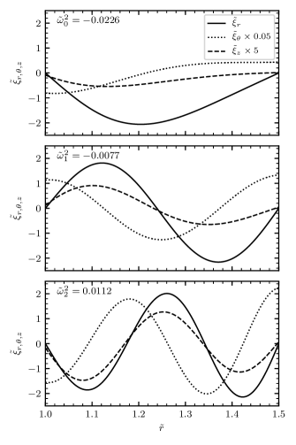
Figure 1: Dimensionless displacement eigenfunctions of the $n=0,1,2$ modes (top to bottom), for an azimuthal wavenumber $m=1$ and an axial wavenumber $k=25$, and an equilibrium model having $\beta=5$, $q=0.01$ and $\gamma=5/3$. In each panel, the eigenfunctions are normalized such that the root-mean-square value of $\tilde{\xi}_{r}$ is unity. The plots are labeled with the corresponding eigenvalue $\tilde{\omega}^{2}_{n}$; negative values for the $n=0$ and $n=1$ modes indicates that they are unstable.

5.3 Dependence on Axial Wavenumber

We now explore how the mode eigenvalues depend on the axial wavenumber $k$. With other parameters fixed at the values given in Section 5.2, Fig. 2 plots the eigenvalues of unstable modes as a function of $k$. The plot shows that for modes with a given radial order $n$ to become unstable, $k$ must exceed some finite threshold $k_{n}$. Above this threshold, the eigenvalue decreases monotonically with $k$, approaching an asymptotic limit as $k\rightarrow\infty$. This is similar behavior to that found by Pitts & Tayler (1985) for a uniform-density incompressible fluid without gravity. In a non-ideal fluid with one or more forms of diffusion (thermal, viscous, or resistive) diffusive damping is expected to reduce the instability of modes at high $k$, leading to a minimal $\tilde{\omega}^{2}<0$ (i.e., maximal growth rate) at large but finite $k$.

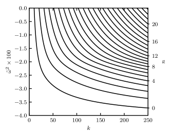
Figure 2: Eigenvalues $\tilde{\omega}^{2}$ plotted as a function of axial wavenumber $k$, for an azimuthal wavenumber $m=1$ and an equilibrium model having $\beta=5$, $q=0.01$ and $\gamma=5/3$. Selected modes are labeled at right with their radial order $n$.

5.4 Stability Boundaries

Because the fundamental mode is the most unstable at any $k$, we can use it as a proxy for the onset of the TI. Accordingly, we evaluate the minimal eigenvalue $\tilde{\omega}_{\rm min}^{2}$, over all modes, as the limiting value of the fundamental-mode eigenvalue in the limit $k\rightarrow\infty$:

$$\tilde{\omega}_{\rm min}^{2}=\lim_{k\rightarrow\infty}\tilde{\omega}_{0}^{2}.$$ (56)

When $\tilde{\omega}_{\rm min}^{2}<0$, the maximal exponential growth rate of the Tayler instability is then given by

$$\lambda_{\rm max}=\frac{a|\tilde{\omega}_{\rm min}|}{r_{0}}.$$ (57)

Because our numerical calculations are restricted to finite values of $k$, we estimate the limit on the right-hand side of equation (56) by evaluating $\tilde{\omega}_{0}^{2}$ at $k=1,000$ and $k=2,000$, and then linearly extrapolating in inverse wavenumber $k^{-1}$ to find the eigenvalue at $k^{-1}\rightarrow 0$.

We apply this approach to evaluate $\tilde{\omega}_{\rm min}^{2}$ for a grid of equilibrium models spanning $1\leq\beta\leq 30$ and $0.00\leq q\leq 0.40$. In all cases, we assume an azimuthal wavenumber $m=1$ and $\gamma=5/3$. Fig. 3 shows a contour map of the resulting values. Plotted over the map are the stability boundaries predicted by the original stability criteria (equation 53), the cTI criteria (equation 54) and the anTI criteria (equation 55). The original criteria over-predict the extent of the instability seen in the numerical calculations, while the cTI criteria under-predict it. Only the anTI criteria correctly predict the stability boundary $\tilde{\omega}_{\rm min}^{2}=0$, confirming that they are the correct choice for LBR anelastic MHD.

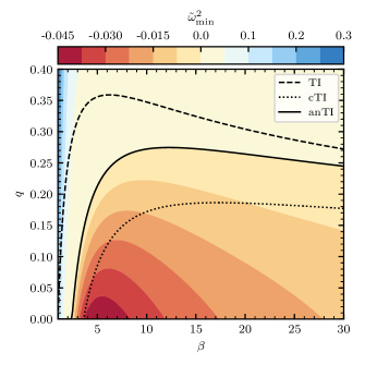
Figure 3: Contour map of the minimal eigenvalue $\tilde{\omega}_{\rm min}^{2}$, plotted across the $\beta$-$q$ plane for an azimuthal wavenumber $m=1$ and equilibrium models having $\gamma=5/3$. Regions where $\tilde{\omega}_{\rm min}^{2}<0$ are unstable to the Tayler instability. The three black lines show the stability boundaries for the fully compressible criteria (TI), the constrained anelastic criteria (cTI) and the LBR anelastic criteria (anTI). Only the LBR anelastic criteria correctly predict the $\tilde{\omega}_{\rm min}^{2}=0$ stability boundary.

In his dynamo models, Spruit (1999, 2002) assumes that the growth rate of the TI is of the order $\lambda\approx\omega_{\rm A}$ in the limit where the rotation angular frequency $\Omega$ is small compared to the Alfvén frequency $\omega_{\rm A}$ defined by

$$\omega_{\rm A}^{2}=\frac{2m^{2}a^{2}}{\beta r^{2}}.$$ (58)

To compare this assumption against our calculations, we write the ratio of growth rate to Alfvén frequency as

$$\frac{\lambda}{\omega_{\rm A}}=|\omega|\sqrt{\frac{\beta r^{2}}{2m^{2}a^{2}}}\lesssim|\tilde{\omega}_{\rm min}|\,\sqrt{\frac{\beta(\tilde{r}_{\rm a}+\tilde{r}_{\rm b})^{2}}{8m^{2}}},$$ (59)

where the second (in)equality follows from setting $|\tilde{\omega}|=|\tilde{\omega}_{\rm min}|$, and evaluating the ratio at the midpoint $\tilde{r}=(\tilde{r}_{\rm a}+\tilde{r}_{\rm b})/2$ of the calculation domain. For modes with azimuthal order $m=1$, we find this ratio has an average value $\lambda/\omega_{\rm A}\approx 0.27$ over the unstable region plotted in Fig. 3, and a maximal value $\lambda/\omega_{\rm A}\approx 0.42$. These are both moderately smaller than the $\lambda/\omega_{\rm A}\approx 1$ assumed by Spruit (1999, 2002). Therefore, future studies involving anelastic MHD simulations of the TI should recognize that the growth rate can be smaller than $\omega_{\rm A}$, and adjust expectations accordingly.

6 Conclusion

The TI is of interest in the radiative regions of stars because, with differential rotation, it may contribute to forming and maintaining a magnetic field dynamo that could significantly affect the stars’ structure and evolution. However, attempts to heuristically derive and numerically simulate the growth and saturation of the TI in stellar models have led to indeterminate results.

The TI criteria were derived using fully compressible MHD, but simulations of fluid dynamics in stellar interiors frequently use some version of the anelastic or pseudo-incompressible approximations, which suppress acoustic waves with much shorter periods than stellar timescales. The goal of this paper was not to address the problem of whether the dynamo exists, but to narrow the gap between fully-compressible linear theory and anelastic non-linear simulations of the TI.

We undertook this by modifying the classic MHD energy principle (Bernstein et al., 1958) according to LBR anelastic MHD, which — based on the work of Brown et al. (2012) — we regard as the most promising of several anelastic schemes. We derived a version of the MHD energy principle that yields stability criteria (equations 46 and 47) in excellent agreement with solutions of the eigenvalue problem calculated using the GYRE code. Our test configuration was a family of cylindrically symmetric magnetohydrostatic equilibria with a toroidal background magnetic field and gravity supplied by a line mass (Section 5.1). Our results show that the instability still exists in LBR anelastic MHD, but in a more restricted part of parameter space than the fully-compressible case. This is because the energy principle is based on minimizing the potential energy of the system, and anelasticity introduces a constraint which precludes full minimization. However, we conclude that the instability should manifest in anelastic LBR MHD simulations if the models used are unstable under the anTI criteria.

We found that the amplitude of the displacement in the horizontal direction is greater than the displacement in the radial direction, as predicted by Spruit (2002). We also found that the largest growth rates calculated by GYRE are somewhat smaller than predicted for slow rotators by Spruit (2002).

We are limited in addressing discrepancies between our calculations and heuristic predictions of the saturated state because our analysis and numerical calculations are in the linear regime and lack rotation or dissipative effects, both of which are key ingredients in the proposed instability-driven dynamo (Spruit, 2002). We are unable to predict the non-linear growth rate and amplitude of the instabilities without taking those physical effects into consideration. That is beyond the scope of this work, but it is an open question for future work.

Our family of cylindrical models can be implemented in anelastic MHD simulations. Such simulations could verify the linear analysis and calculations that we performed, and determine how non-linear effects impact the growth rate and amplitude of the instability. Choosing models that are unstable under the anTI criteria, and including differential rotation, anelastic MHD simulations could more accurately test the the Tayler-Spruit dynamo and its significance as a mechanism for angular momentum transport in stellar evolution.

7 Acknowledgements

Our work made possible through the collaborative effort of the Supernova Progenitors, Internal Dynamics and Evolution Research (SPIDER) network, supported via NASA TCAN program grant NNX14AB55G. We also acknowledge support from NSF grants AST-1716436, PHY-1748958 and ACI-1663696, and from the Wisconsin Alumni Research Foundation. We thank Ryan Orvedahl and Benjamin Brown for their help using Dedalus (http://dedalus-project.org) to verify the initial GYRE calculations, and Erin Boettcher for her thorough review. EGZ thanks the University of Chicago for hospitality during the completion of this manuscript. We thank the referee for the useful comments that led to significant improvements in the paper.

Appendix A Numerical Technique

To calculate numerical solutions of the LBR anelastic equations (19–23,26), we first undertake a separation of variables in space and time, by writing perturbed quantities in the form

$$\begin{pmatrix}\xi_{r}\\ \xi_{\phi}\\ \xi_{z}\end{pmatrix}=r_{0}\operatorname{Re}\left\{\begin{pmatrix}\tilde{\xi}_{r}\\ \mathrm{i}\tilde{\xi}_{\phi}\\ \mathrm{i}\tilde{\xi}_{z}\end{pmatrix}\exp[\mathrm{i}(m\phi+kz/r_{0}+\omega t)]\right\}$$ (A1)

$$\begin{pmatrix}B_{r}^{\prime}\\ B_{\phi}^{\prime}\\ B_{z}^{\prime}\end{pmatrix}=\sqrt{\frac{8\pi P_{0}}{\beta}}\operatorname{Re}\left\{\begin{pmatrix}\mathrm{i}\tilde{B}_{r}^{\prime}\\ \tilde{B}_{\phi}^{\prime}\\ \tilde{B}_{z}^{\prime}\end{pmatrix}\exp[\mathrm{i}(m\phi+kz/r_{0}+\omega t)]\right\}$$ (A2)

$$\begin{pmatrix}J_{r}^{\prime}\\ J_{\phi}^{\prime}\\ J_{z}^{\prime}\end{pmatrix}=\frac{c}{4\pi r_{0}}\sqrt{\frac{8\pi P_{0}}{\beta}}\operatorname{Re}\left\{\begin{pmatrix}\mathrm{i}\tilde{J}_{r}^{\prime}\\ \tilde{J}_{\phi}^{\prime}\\ \tilde{J}_{z}^{\prime}\end{pmatrix}\exp[\mathrm{i}(m\phi+kz/r_{0}+\omega t]\right\}.$$ (A3)

$$\Pi^{\prime}=\frac{P_{0}}{\rho_{0}}\operatorname{Re}\left\{\tilde{\Pi}^{\prime}\exp[\mathrm{i}(m\phi+kz/r_{0}+\omega t]\right\}$$ (A4)

$$S^{\prime}=c_{P}\operatorname{Re}\left\{\tilde{S}^{\prime}\exp[\mathrm{i}(m\phi+kz/r_{0}+\omega t]\right\}$$ (A5)

In these expressions, all quantities with a tilde (~) are dimensionless real functions of $r$, to be determined numerically; the integer $m$ is the azimuthal wavenumber introduced in Section (4.1), and the real number $k$ is the axial wavenumber. Here, we choose to work with

$$\Pi^{\prime}=\varpi^{\prime}+\frac{B_{\phi}B_{\phi}^{\prime}}{4\pi\rho_{0}}.$$ (A6)

rather than the reduced pressure $\varpi$, as this allows $\tilde{J}_{\phi}^{\prime}$ and $\tilde{J}_{z}^{\prime}$ to be decoupled from the other dependent variables, reducing the differential order of the system from four to two.

With these definitions, and assuming the equilibrium we introduce in Section 5.1, we write the linearized equations in the form

$$\frac{\mathrm{d}\boldsymbol{v}}{\mathrm{d}\tilde{r}} =\boldsymbol{\mathsf{A}}_{vv}\boldsymbol{v}+\boldsymbol{\mathsf{A}}_{vw}\boldsymbol{w}$$ (A7)

$$\boldsymbol{0} =\boldsymbol{\mathsf{A}}_{wv}\boldsymbol{v}+\boldsymbol{\mathsf{A}}_{ww}\boldsymbol{w}$$ (A8)

where $\tilde{r}\equiv r/r_{0}$ is the independent variable, and the vectors

$$\boldsymbol{v}=\begin{pmatrix}\tilde{\xi}_{r}\\ \tilde{\Pi}^{\prime}\end{pmatrix},\qquad\boldsymbol{w}=\begin{pmatrix}\tilde{\xi}_{\phi}\\ \tilde{\xi}_{z}\\ \tilde{B}_{r}^{\prime}\\ \tilde{B}_{\phi}^{\prime}\\ \tilde{B}_{z}^{\prime}\\ \tilde{J}_{r}^{\prime}\\ \tilde{S}^{\prime}\end{pmatrix}$$ (A9)

contain the dependent variables. The Jacobian matrices in equations (A7) and (A8) are given by

$$\boldsymbol{\mathsf{A}}_{vv}=\begin{pmatrix}\frac{\alpha-1}{\tilde{r}}&0\\ \tilde{\omega}^{2}&0\end{pmatrix},$$ (A10)

$$\boldsymbol{\mathsf{A}}_{vw}=\begin{pmatrix}\frac{m}{\tilde{r}}&k&0&0&0&0&0\\ 0&0&-\frac{2m}{\beta\tilde{r}}&\frac{2(\alpha-2)}{\beta\tilde{r}}&0&0&\frac{q}{\tilde{r}}\end{pmatrix},$$ (A11)

$$\boldsymbol{\mathsf{A}}_{wv}=\begin{pmatrix}0&-\frac{m}{\tilde{r}}\\ 0&-k\\ \frac{m}{\tilde{r}}&0\\ \frac{2-\alpha}{2\tilde{r}}&0\\ 0&0\\ 0&0\\ \frac{\alpha(\gamma-1)}{\gamma\tilde{r}}&0\end{pmatrix},$$ (A12)

$$\boldsymbol{\mathsf{A}}_{ww}=\begin{pmatrix}\tilde{\omega}^{2}&0&\frac{2-\alpha}{\beta\tilde{r}}&\frac{2m}{\beta\tilde{r}}&0&0&0\\ 0&\tilde{\omega}^{2}&0&\frac{2k}{\beta}&0&\frac{2}{\beta}&0\\ 0&0&-1&0&0&0&0\\ -\frac{m}{\tilde{r}}&0&0&-1&0&0&0\\ 0&-\frac{m}{\tilde{r}}&0&0&-1&0&0\\ 0&0&0&-k&\frac{m}{\tilde{r}}&-1&0\\ 0&0&0&0&0&0&1\end{pmatrix},$$ (A13)

where we introduce the dimensionless frequency

$$\tilde{\omega}=\frac{r_{0}}{a}\omega.$$ (A14)

Eliminating $\boldsymbol{w}$ between equations (A7) and (A8), we arrive at a system of differential equations for $\boldsymbol{v}$ alone:

$$\frac{\mathrm{d}\boldsymbol{v}}{\mathrm{d}\tilde{r}}=\left(\boldsymbol{\mathsf{A}}_{vv}-\boldsymbol{\mathsf{A}}_{vw}\boldsymbol{\mathsf{A}}_{ww}^{-1}\boldsymbol{\mathsf{A}}_{wv}\right)\boldsymbol{v}\equiv\boldsymbol{\mathsf{A}}\boldsymbol{v},$$ (A15)

where the second equality serves to define the overall Jacobian matrix $\boldsymbol{\mathsf{A}}$. Although we do not write out an explicit expression for the elements of $\boldsymbol{\mathsf{A}}$, we note that each contains a factor

$$F=\frac{1}{\beta\tilde{r}^{2}\tilde{\omega}^{2}-2m^{2}}=\frac{1}{\beta\tilde{r}^{2}(\tilde{\omega}^{2}-\tilde{\omega}_{\rm A}^{2})},$$ (A16)

where

$$\tilde{\omega}_{\rm A}=\frac{r_{0}}{a}\omega_{\rm A}$$ (A17)

is the dimensionless equivalent of the Alfvén frequency defined in equation (58). The factor $F$ diverges if $\tilde{\omega}=\tilde{\omega}_{\rm A}$, indicating a local resonance with the Alfvén wave. In the present context, such behavior is not a problem because we are interested in finding unstable modes for which $\tilde{\omega}^{2}<0$, and therefore the resonance never arises.

Together with the boundary conditions

$$v_{1}=\tilde{\xi}_{r}=0$$ (A18)

on the inner ($\tilde{r}=\tilde{r}_{\rm a}$) and outer ($\tilde{r}=\tilde{r}_{\rm b}$) boundaries of the calculation domain (in accordance with equation 32), the system of equations (A15) is a linear two-point boundary eigenvalue problem (BVEP), with $\tilde{\omega}^{2}$ serving as the eigenvalue. To solve the BVEP numerically we use the GYRE code (Townsend & Teitler, 2013). Although GYRE is designed to address stellar pulsation problems, it is built on a robust multiple-shooting scheme which can in principle be applied to any BVEP. Accordingly, we modify GYRE to implement the differential equations and boundary conditions given here. The modified code takes as inputs parameters specifying the equilibrium model ($\beta,\gamma,q$), the wavenumbers ($m,k$), and the calculation domain ($\tilde{r}_{\rm a},\tilde{r}_{\rm b}$, and the number of points $N$ used to discretize the differential equations). As outputs, it calculates the eigenvalues $\tilde{\omega}^{2}$ of the discrete modal solutions, and the corresponding eigenfunctions given by the components of $\boldsymbol{v}$ and $\boldsymbol{w}$.

References

- Acheson (1978) Acheson, D. J. 1978, Phil. Trans. Roy. Soc. London A, 289, 459
- Aurière et al. (2007) Aurière, M., Wade, G. A., Silvester, J., et al. 2007, A&A, 475, 1053
- Bernstein et al. (1958) Bernstein, I. B., Frieman, E. A., Kruskal, M. D., & Kulsrud, R. M. 1958, Proc. Roy. Soc. London A, 244, 17
- Braginsky & Roberts (1995) Braginsky, S. I., & Roberts, P. H. 1995, Geophysical and Astrophysical Fluid Dynamics, 79, 1
- Braithwaite (2006a) Braithwaite, J. 2006a, A&A, 453, 687
- Braithwaite (2006b) —. 2006b, A&A, 449, 451
- Brown et al. (2012) Brown, B. P., Vasil, G. M., & Zweibel, E. G. 2012, ApJ, 756, 109
- Cantiello et al. (2014) Cantiello, M., Mankovich, C., Bildsten, L., Christensen-Dalsgaard, J., & Paxton, B. 2014, ApJ, 788, 93
- Denissenkov & Pinsonneault (2007) Denissenkov, P. A., & Pinsonneault, M. 2007, ApJ, 655, 1157
- Fuller et al. (2019) Fuller, J., Piro, A. L., & Jermyn, A. S. 2019, MNRAS, 485, 3661
- Heger et al. (2005) Heger, A., Woosley, S. E., & Spruit, H. C. 2005, ApJ, 626, 350
- Kulsrud (1964) Kulsrud, R. 1964, in Astrophysics Today, Vol. 63, Advanced Plasma Theory, ed. M. N. Rosenbluth, 54
- Lantz (1992) Lantz, S. R. 1992, PhD thesis, Cornell University
- Maeder & Meynet (2003) Maeder, A., & Meynet, G. 2003, A&A, 411, 543
- Maeder & Meynet (2004) —. 2004, A&A, 422, 225
- Maeder & Meynet (2005) —. 2005, A&A, 440, 1041
- Markey & Tayler (1973) Markey, P., & Tayler, R. J. 1973, MNRAS, 163, 77
- Markey & Tayler (1974) —. 1974, MNRAS, 168, 505
- Meynet & Maeder (2005) Meynet, G., & Maeder, A. 2005, A&A, 429, 581
- Paxton et al. (2013) Paxton, B., Cantiello, M., Arras, P., et al. 2013, ApJS, 208, 4
- Paxton et al. (2015) Paxton, B., Marchant, P., Schwab, J., et al. 2015, ApJS, 220, 15
- Paxton et al. (2018) Paxton, B., Schwab, J., Bauer, E. B., et al. 2018, ApJS, 234, 34
- Pitts & Tayler (1985) Pitts, E., & Tayler, R. J. 1985, MNRAS, 216, 139
- Song et al. (2016) Song, H. F., Meynet, G., Maeder, A., Ekström, S., & Eggenberger, P. 2016, A&A, 585, A120
- Song et al. (2018) Song, H. F., Meynet, G., Maeder, A., et al. 2018, A&A, 609, A3
- Spruit (1999) Spruit, H. C. 1999, A&A, 349, 189
- Spruit (2002) —. 2002, A&A, 381, 923
- Tayler (1973) Tayler, R. J. 1973, MNRAS, 161, 365
- Townsend & Teitler (2013) Townsend, R. H. D., & Teitler, S. A. 2013, MNRAS, 435, 3406
- Zahn et al. (2007) Zahn, J.-P., Brun, A. S., & Mathis, S. 2007, A&A, 474, 145