$f$-mode strengthening from a localised bipolar subsurface magnetic field

Abstract

Recent numerical work in helioseismology has shown that a periodically varying subsurface magnetic field leads to a fanning of the $f$-mode, which emerges from a density jump at the surface. In an attempt to model a more realistic situation, we now modulate this periodic variation with an envelope, giving thus more emphasis on localised bipolar magnetic structures in the middle of the domain. Some notable findings are: (i) compared to the purely hydrodynamic case, the strength of the $f$-mode is significantly larger at high horizontal wavenumbers $k$, but the fanning is weaker for the localised subsurface magnetic field concentrations investigated here than the periodic ones studied earlier; (ii) when the strength of the magnetic field is enhanced at a fixed depth below the surface, the fanning of the $f$-mode in the $k\omega$ diagram increases proportionally in such a way that the normalised $f$-mode strengths remain nearly the same in different such cases; (iii) the unstable Bloch modes reported previously in case of harmonically varying magnetic fields are now completely absent when more realistic localised magnetic field concentrations are imposed beneath the surface, thus suggesting that the Bloch modes are unlikely to be supported during most phases of the solar cycle; (iv) the $f$-mode strength appears to depend also on the depth of magnetic field concentrations such that it shows a relative decrement when the maximum of the magnetic field is moved to a deeper layer. We argue that detections of $f$-mode perturbations such as those being explored here could be effective tracers of solar magnetic fields below the photosphere before these are directly detectable as visible manifestations in terms of active regions or sunspots.

1 Introduction

The Sun supports a wide variety of waves that carry useful information about the internal solar structure, which can be inferred by employing the methods of helioseismology (see, e.g., Gough, 1987; Christensen-Dalsgaard, 2003). Local analysis using especially the surface gravity mode (or the $f$-mode) is useful in studying the near-surface structure (e.g. Hanasoge et al., 2008; Felipe et al., 2012, 2013; Daiffallah et al., 2011). Some properties of surface waves in idealised settings involving magnetic fields were explored in Chandrasekhar (1961); Roberts (1981); Miles & Roberts (1989, 1992); Miles et al. (1992). It is of great interest to probe interior magnetic fields of the Sun using the techniques of helioseismology; see Thompson (2006) for a review on the subject of magnetohelioseismology. Systematic changes, notably in the frequencies of the global $f$-mode, as a function of solar cycle were found and discussed in detail in Thompson (2006) and Pintér (2008). Thompson (2006) found evidence of a $500\,{\rm G}$ magnetic field at a depth of about $5\,{\rm Mm}$ and suggested $2\%$ modulation in turbulent convection velocities from solar minimum to maximum, based on the observed cycle-dependence of mean frequency shifts of the $f$- and $p$-modes. Moreover, it is reasonable to expect magnetically induced variations in the $f$-mode on much shorter timescales, e.g., during localised magnetic flux emergence leading to the formation of active regions (ARs) or sunspots.

Much of the earlier studies on the global $f$-mode of the Sun focussed primarily on the frequency shifts that were observed (Libbrecht et al., 1990; Fernandes et al., 1992). The frequencies were significantly smaller than the theoretically expected values, where both the shift and line width grow with the spherical harmonic degree. Subsequent studies explained these findings by invoking turbulent background motions and deriving a generalised dispersion relation of the $f$-mode in the presence of a random velocity field (Murawski & Roberts, 1993a, b; Mȩdrek et al., 1999; Murawski, 2000a, b; Mole et al., 2008). The influence of coherent (for modelling supergranulation) as well as random (mimicking near-surface granulation) flows on the $f$-mode were explored in detail by Murawski (2000a) where it was found that, while a space-dependent random flow causes a decrement, a time-dependent random flow can enhance the frequencies. Observations were thus explained in terms of the parameters of the chosen velocity field. However, these studies ignored the effect of magnetic fields, which can increase the $f$-mode frequencies (e.g. Chandrasekhar, 1961; Roberts, 1981; Miles & Roberts, 1992; Miles et al., 1992).

In a series of works, Cally & Bogdan (1993, 1997) and Cally et al. (1994) investigated the interaction of $f$- and $p$-modes with a vertical magnetic field and found that a partial conversion of these modes into slow magnetoacoustic modes takes place whenever they encounter a vertical field resembling those of sunspots. Parchevsky & Kosovichev (2009) numerically explored the effects of inclined magnetic fields and noted that the $f$-modes are more strongly affected by the background magnetic field than the $p$-modes. Singh et al. (2015) studied numerically various properties of the $f$- as well as $p$- and $g$-modes in a wide variety of magnetic backgrounds. They found that horizontal magnetic fields cause an increase in the $f$-mode frequencies – as expected. But their dependencies are more complicated in the presence of vertical or oblique magnetic fields, which may be more relevant for the predominantly vertical fields of sunspots. In this case, the $f$-mode frequencies are enhanced relative to their nonmagnetic values at intermediate horizontal wavenumbers, but decreased at large wavenumbers.

In the presence of magnetic fields in the solar atmosphere, Alfvén and magnetosonic waves are known to couple resonantly with the global oscillations, affecting mainly the frequencies, line widths, and penetration of the $f$ and $p$ modes into the solar atmosphere (see Erdélyi, 2006, for a review and references therein). Another important finding was that resonant interaction between global modes and Alfvén waves causes a damping of the $f$- and $p$-modes due to dissipative effects near the resonance frequency. Pintér & Erdélyi (2018) further study this situation by deriving the dispersion relation of the $f$-mode in a magnetically coupled solar interior-atmosphere system to obtain its frequency shifts. For a magnetised atmosphere, these were found to be positive relative to an unmagnetised one.

It is of great interest to use numerical simulations to study the effects of subsurface magnetic fields on both the acoustic or $p$-modes and the $f$-mode. Such studies aim at refining the interpretation of helioseismic measurements which use sound waves to infer the internal structure of the Sun and its internal motions (e.g. Basu, 2016; Hanasoge et al., 2016). This is necessary, because magnetic fields complicate the usage of helioseismic inversion techniques, as their presence gives rise to the modification of sound and gravity waves into magnetoacoustic and magnetogravity ones which are difficult to account for (Thomas, 1983; Campos, 2011). Furthermore, if the properties and behaviour of $p$- and $f$-modes in the presence of magnetic fields of different strength, topology or location, in particular depth, were known well enough from the numerical models, we might be able to infer the subsurface magnetic fields from helioseismic measurements. From such inferences, we may be able to learn about the origin of subsurface magnetic fields, that is, about the solar dynamo mechanism (Brandenburg, 2005; Charbonneau, 2010; Käpylä et al., 2012), and about the process of concentrating magnetic fields into sunspots and ARs; see, e.g., Brandenburg et al. (2016) and Käpylä et al. (2016) for a competing mechanism enabling a self-consistent formation of localised magnetic flux concentrations.

Such numerical simulations, enabling us to study the effects of magnetic fields on the naturally occurring modes of oscillations, have recently been performed with the Pencil Code. Singh et al. (2015) introduced a modelling framework with a piecewise isothermal atmosphere, where the upper layer is mimicking a hot corona and the lower one a (cooler) convection zone. The two layers are separated by a jump in density and temperature, which represents the solar surface and enables the presence of the $f$-mode. For a simple approximation of the convective turbulence, random hydrodynamic forcing was applied in the lower layer. In such a setup, acoustic ($p$), internal gravity ($g$), and surface gravity ($f$) modes are all self-consistently driven, in contrast to other types of approaches, which selectively produce the modes based on linearised equations (Daiffallah et al., 2011; Schunker et al., 2011). Singh et al. (2015) studied the influence of uniformly imposed magnetic fields on the $p$- and $f$-mode properties, and verified the expectation of $f$-modes being sensitive to the presence of magnetic fields and $p$-modes being less affected. The major effect on the $f$-modes was an increase in their mode frequencies. Singh et al. (2014) developed the setup further to include non-uniform magnetic fields with harmonic profiles within the convection zone. This work revealed the fanning effect of the $f$-mode, that is, an increase of its line width towards higher wavenumbers. The width of the fan and its asymmetry could be directly related to the strength and location of the magnetic field.

These numerical studies and their predictions led to an observational case study of $f$-modes in relation to the emergence of about half a dozen ARs, observed with HMI, and the resulting line-of-sight Dopplergrams and magnetograms (Singh et al., 2016). This study reported strengthening of the local $f$-mode about two days before the emergence of ARs at the same corotating patch. It was noted that such a precursor signal can be detected by isolating high-degree $f$-modes through careful fitting and subsequent subtraction of background and $p$-modes. It was argued there that the precursor signal is best seen when an AR forms in isolation, i.e., far from other existing ARs which can ‘pollute’ the signal. It is known that the sunspots or ARs absorb the $f$-mode power, thus causing its damping (Cally & Bogdan, 1997), and therefore it is expected to be harder to extract the precursor signal associated with a newly forming AR in a ‘crowded’ environment with many existing ARs. A possible cleaning procedure to still extract the signal was discussed in Singh et al. (2016). Although this is yet to be confirmed for larger data sets and with independent observational techniques, the potential significance of such $f$-mode related precursors cannot be understated. Based on the photospheric velocity measurements, Khlystova & Toriumi (2017) detected plasma upflows somewhat before the emergence of two small ARs. A number of previous case studies have reported detections of subphotospheric velocities associated with emerging ARs using different techniques, such as, helioseismic holography, ring-diagram or time-distance analysis (Komm et al., 2008; Hartlep et al., 2011; Ilonidis et al., 2011; Birch et al., 2013; Barnes et al., 2014). Given that the $f$-mode eigenfunctions extend to depths of about a few Mm, it might be expected to be sensitive to such velocity perturbations.

In this paper we extend the model of Singh et al. (2014, 2015) to study the $f$-mode strengthening and fanning using inhomogeneous magnetic fields of different strength, topology, and location in the convection zone. In addition to using harmonic profiles which stretch over the whole horizontal extent, we use localised harmonic perturbations, to better mimic isolated active regions. We describe our model and basic definitions in section 2 and present our results in section 3. Conclusions are given in section 4.

2 Model setup and analysis technique

We consider here a model that is similar to that studied in Singh et al. (2014, 2015). The $p$-, $g$- and $f$-modes are produced in a self-consistent manner in a two-dimensional Cartesian $x$-$z$ domain with a piecewise isothermal medium consisting of a cool lower layer, called bulk, and a hotter upper layer, called corona. The thicknesses of these layers are $L_{\rm d}$ and $L_{\rm u}$, respectively, where subscripts ‘d’ and ‘u’ refer to the layers downward and upward of the interface. A non-uniform magnetic background field is maintained by including an electromotive force (EMF) in the uncurled version of the induction equation for the magnetic vector potential $\bm{A}$. We solve the basic hydromagnetic equations,

$$\frac{D\ln\rho}{Dt} =-\bm{\nabla}\cdot\bm{u},$$ (1)

$$\frac{D\bm{u}}{Dt} =\mbox{\boldmath$f$}{}+\bm{g}+\frac{1}{\rho}\left(\bm{J}\times\bm{B}-\bm{\nabla}p+\bm{\nabla}\cdot 2\nu\rho\bm{\mathsf{S}}\right),$$ (2)

$$T\frac{Ds}{Dt} =2\nu\bm{\mathsf{S}}^{2}+\frac{\mu_{0}\eta}{\rho}\bm{J}^{2}-(\gamma-1)c_{p}\frac{T-T_{\rm d,u}}{\tau_{\rm c}}\,,$$ (3)

$$\frac{\partial\bm{A}}{\partial t} ={\bm{u}}\times{\bm{B}}+\mbox{\boldmath${\cal E}$}{}_{0}-\eta\mu_{0}{\bm{J}},$$ (4)

where $\rho$ is the density, $\bm{u}$ is the velocity, $D/Dt=\partial/\partial t+\bm{u}\cdot\bm{\nabla}$ is the advective time derivative, $\bm{f}$ is a forcing function [as specified in Brandenburg (2001)] to drive seismic modes of low Mach number, $\bm{g}=(0,0,-g)$ is the gravitational acceleration, $\mathsf{S}_{ij}={\textstyle{1\over 2}}(u_{i,j}+u_{j,i})-{\textstyle{1\over 3}}\delta_{ij}\bm{\nabla}\cdot\bm{u}$ is the traceless rate of strain tensor, with commas denoting partial differentiation, $\nu={\rm const}{}$ is the kinematic viscosity, ${\bm{B}}=\bm{\nabla}\times{\bm{A}}$ is the magnetic field, ${\bm{J}}=\mu_{0}^{-1}\bm{\nabla}\times{\bm{B}}$ is the current density, $\mu_{0}$ is the vacuum permeability, $s$ is the specific entropy, $\gamma=c_{\rm p}/c_{\rm v}$ is the ratio of specific heats at constant pressure and volume, respectively, $T$ is the temperature, $\mbox{\boldmath${\cal E}$}{}_{0}$ is an external EMF specified below, and $\eta={\rm const}{}$ is the magnetic diffusivity. Since the forcing amplitude is small, no additional hyperdiffusion is needed, and also no diffusion in the energy equation was included. The fluid is assumed to obey the equation of state of an ideal gas, hence the pressure is given by $p=(c_{\rm p}-c_{\rm v})\rho T=\rho c_{\rm s}^{2}/\gamma$. The medium is vertically stratified under constant gravity, $g>0$, where we identify $x$ and $z$ as horizontal and vertical directions, respectively. All calculations are performed with the Pencil Code.

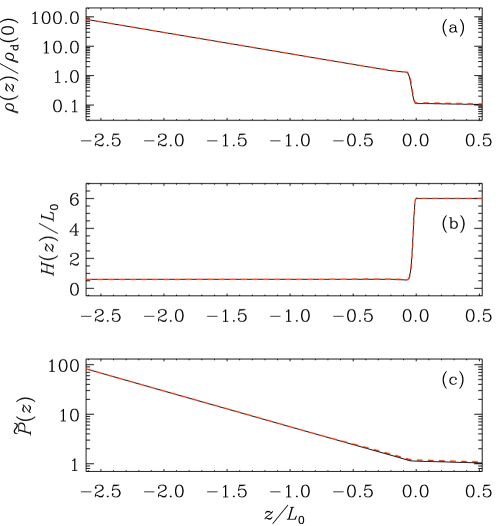
Figure 1: Density (a), scale height (b), and pressure (c) of the horizontally averaged background state as functions of $z$, where $\tilde{P}=\gamma P/\rho_{\rm d}(0)c_{\rm sd}^{2}$. Solid, black: hydro (H1); dashed, red: magnetic (A1) case.

The variations of background density, pressure scale height, and pressure as functions of $z$ are shown in figure 1. Similar to earlier works (Singh et al., 2014, 2015) we introduce a sharp jump in density at the interface $z=0$ with $\rho_{\rm u}(0)\ll\rho_{\rm d}(0)$, along with corresponding jumps in temperature. The adiabatic sound speed $c_{\rm s}$ is maintained by the last term in equation (3), which guarantees the relaxation to constant average temperatures $T_{\rm d}$ and $T_{\rm u}$ in either subdomain within a relaxation time $\tau_{\rm c}$ (constant throughout the domain). In this way, the interface is created and maintained and the $f$-mode is naturally enabled. It is therefore also known as the free surface mode. As the density decreases exponentially with height $z$ in an isothermally stratified medium, it is given by $\rho_{\rm d,u}(z)=\rho_{\rm d,u}(0)\exp(-z/H_{\rm d,u})$, where $H_{\rm d,u}=(c_{\rm p}-c_{\rm v})T_{\rm d,u}/g$ is the scale height. (The pressure and density scale heights are equal for an isothermal layer.) The sharp jump in the thermodynamic quantities is quantified by the ratio

$$q=\frac{\rho_{\rm u}(0)}{\rho_{\rm d}(0)}=\frac{c_{\rm sd}^{2}}{c_{\rm su}^{2}}=\frac{T_{\rm d}}{T_{\rm u}}=\frac{H_{\rm d}}{H_{\rm u}}.$$ (5)

We enforce a steady magnetic field $\bm{B}_{0}$ by applying a constant external EMF $\mbox{\boldmath${\cal E}$}{}_{0}={\cal E}_{0y}^{\rm A,B}\mbox{\boldmath$e$}{}_{y}$. Two different types of magnetic structures are considered in the magnetohydrodynamic (MHD) simulations, called models A and B. Model A is characterized by a harmonic variation in both spatial dimensions

$${\cal E}_{0y}^{\rm A}=\hat{\cal E}_{0}\cos\left(k^{B}_{x}x\right)\cos\left(k^{B}_{z}z\right),$$ (6)

and model B by a localised sine wave

$${\cal E}_{0y}^{\rm B}=\hat{\cal E}_{0}{\cal F}^{\rm TH}(x;x_{1},x_{2})\sin\left(k^{B}_{x}x\right)\exp{\left[-\left(\frac{z-z_{*}}{w_{z}}\right)^{2}\right]}\,,$$ (7)

where ${\cal F}^{\rm TH}(x;x_{1},x_{2})$ is a smoothed top hat as a function of $x$, centred w.r.t. $x$. It is unity for $x\in[x_{1},x_{2}]$ and smoothly goes to zero outside this interval; see, e.g., figures 4 and 5 for the profiles of the imposed magnetic background in its saturated state. The transitions at $x_{1}$ and $x_{2}$ are modelled with a third-order polynomial of width $w\approx 0.3H_{\rm d}$. Note that the sustained magnetic field $\bm{B}_{0}$ drives a large-scale flow which, in turn, acts back on the field, so that its shape is not simply determined by $\eta\nabla^{2}\bm{B}_{0}+\nabla\times\mbox{\boldmath${\cal E}$}{}_{0}=\bm{0}$. The A models are very similar to those considered in Singh et al. (2014), whereas the B ones were tailored to model an emerging active region more realistically: given that ARs hardly ever show a periodic pattern in longitude, we restricted the horizontal extent of the subsurface magnetic structures in the B models, mimicking more closely the fields of bipolar regions. Both models allow us to explore the effects of subsurface magnetic fields on the $f$-mode, naturally occurring at the interface in our minimalistic setup. It is nevertheless sufficiently realistic for understanding the solar $f$-mode that is expected to be unaffected by the choice of the thermodynamic background state of the medium. The top and bottom boundaries were chosen to be stress free and perfectly conducting, whereas periodicity was assumed in the horizontal direction.

The length scales and frequencies are normalised by $L_{0}=\gamma H_{\rm d}=c_{\rm sd}^{2}/g$ and $\omega_{0}=g/c_{\rm sd}$, and the dimensionless variables are indicated by tildae, i.e., $\widetilde{k}_{x}=k_{x}L_{0}$, $\widetilde{\omega}=\omega/\omega_{0}$, and so on. From the vertical velocity $u_{z}$ at $z=0$, we construct the diagnostic $k_{x}$-$\omega$ diagram ($k\omega$ diagram for short) by taking the Fourier transform of $u_{z}(x,0,t)$, giving $\hat{u}_{z}(k_{x},\omega)$, which here has the same dimension as velocity. The $k\omega$ diagrams, such as those shown in figure 2 are constructed from the dimensionless quantity

$$\widetilde{P}(k_{x},\omega)=\frac{|\hat{u}_{z}(k_{x},\omega)|}{u_{0}}\,,$$ (8)

where the mass-weighted root-mean-squared (rms) velocity $u_{0}=\sqrt{\langle\rho^{2}u_{\rm d}^{2}\rangle/\langle\rho^{2}\rangle}$ is employed for normalisation and the angle brackets denote volume averaging over the bulk. We define the fluid Reynolds and Mach numbers as $\mbox{\rm Re}=u_{0}/(\nu k_{\rm f})$ and $\mbox{\rm Ma}=u_{0}/c_{\rm sd}$, respectively, where we choose $\widetilde{k}_{\rm f}=20$ for the wavenumber of the hydrodynamic low amplitude nonhelical forcing in equation (2).

Table 1: Summary of all simulations. $\tilde{x}$–$\tilde{z}$ domain: $8\pi\times\pi$; grid: $1024\times 320$; $\mbox{\rm Pr}_{\rm m}=1$; $q=0.11$; $|\mbox{\boldmath$f$}{}|/g=10^{-4}$ for all runs. $\widetilde{k}_{x}^{B}=0.5$, $\widetilde{k}_{z}^{B}=2$ and $\widetilde{w}_{z}=0.28$ were chosen in equations (6) and (7); $\Delta\tilde{x}_{B}=(x_{2}-x_{1})/L_{0}$.

Run	$\tilde{\nu}$	extent of ${\bm{f}}$	Re	Ma	magnetic background				$\Sigma_{\rm f}$
					geometry	$\Delta\tilde{x}_{B}$	$\max(v_{\rm A}/c_{\rm s})$	at depth
H1	$2\times 10^{-4}$	full	0.22	0.00087	–	–	–	–	0.0025
H2	$4\times 10^{-4}$	full	0.08	0.00066	–	–	–	–	0.0022
H3	$4\times 10^{-4}$	$\tilde{z}<0$	0.08	0.00065	–	–	–	–	0.0012
H4	$4\times 10^{-4}$	$\tilde{z}<-0.2$	0.08	0.00063	–	–	–	–	0.0008
A1	$2\times 10^{-4}$	full	0.56	0.0022	Eq. (6)	–	0.15	$1.3H_{\rm d}$	0.0042
A2	$2\times 10^{-4}$	full	0.60	0.0024	Eq. (6)	–	0.18	$1.3H_{\rm d}$	0.0038
A3	$2\times 10^{-4}$	full	0.64	0.0026	Eq. (6)	–	0.24	$1.3H_{\rm d}$	0.0036
A4	$2\times 10^{-4}$	full	0.77	0.0031	Eq. (6)	–	0.29	$1.3H_{\rm d}$	0.0040
BI1	$4\times 10^{-4}$	$\tilde{z}<0$	0.10	0.0008	Eq. (7)	$4\pi$	0.12	$2.4H_{\rm d}$	0.0018
BI2	$4\times 10^{-4}$	$\tilde{z}<0$	0.18	0.0014	Eq. (7)	$4\pi$	0.31	$1.8H_{\rm d}$	0.0046
BII	$4\times 10^{-4}$	$\tilde{z}<-0.2$	0.09	0.0007	Eq. (7)	$7\pi$	0.12	$2.4H_{\rm d}$	0.0010

In order to characterise the strength of the $f$-mode, we determine the normalised mode strength $\mu_{\rm f}$ as a function of $\widetilde{k}_{x}$ by fitting a Lorentzian to the line profile of the $f$-mode along the frequency axis and subtracting the continuum. Here we define the mode strength as

$$\mu_{\rm f}(\widetilde{k}_{x})=\int\Delta\widetilde{P}(\widetilde{k}_{x},\widetilde{\omega})\,{\rm d}{}\widetilde{\omega}\,,$$ (9)

where $\Delta\widetilde{P}$ denotes the normalised excess amplitude of the $f$-mode over the continuum at $\widetilde{k}_{x}$. This yields a wavenumber-dependent mode strength in a manner similar to that used in Singh et al. (2016) where, however, a more involved fitting algorithm was used to isolate the $f$-mode, which lies much closer to the $p$-modes in a more realistic setting with an isentropic stratification. It is useful to define an integrated normalised mode amplitude of the $f$-mode as,

$$\Sigma_{\rm f}=\int\mu_{\rm f}\,{\rm d}{}\widetilde{k}_{x},$$ (10)

which is called here, for short, the relative mode amplitude.

3 Results

We present results from a suite of hydrodynamic (H) as well as MHD runs (Sets A and B) with different geometries of the imposed background magnetic field. We refer the reader to table 1 for the parameters of all simulations.

3.1 Hydrodynamic runs

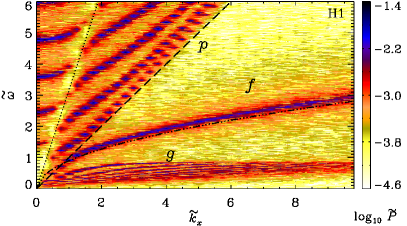
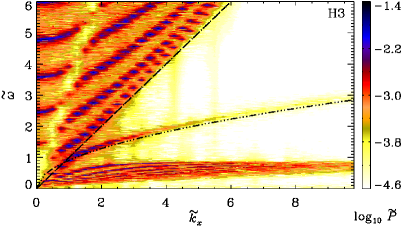
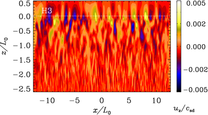
Figure 2: Top: $k\omega$ diagrams for the hydrodynamic runs H1 (left) and H3 (right). The dotted and dashed lines show $\omega=c_{\rm su}k_{x}$ and $\omega=c_{\rm sd}k_{x}$, respectively; the dash-dotted curves show $\omega_{\rm f}(k_{x})$ of the classical $f$-mode. Bottom: normalised mode strength $\mu_{f}$ of the $f$-mode as a function of $\widetilde{k}_{x}$ for the hydrodynamic runs H1–H4 (left), and a snapshot of $u_{z}/c_{\rm sd}$ in the statistically steady state of stochastic motions for the run H3 (right); see table 1 for more details.

We performed four different hydrodynamic runs, H1–H4, to assess the roles of viscosity and vertical extent of $f$. We first show the diagnostic $k\omega$ diagram, which clearly reveals the $p$, $g$, and $f$-modes; see the top left panel of figure 2 for model H1. While the $g$-modes are confined to frequencies $\widetilde{\omega}<1$, the $p$-modes lie above the line $\widetilde{\omega}=\widetilde{k}_{x}$, as already seen in Singh et al. (2015) and as expected in the piecewise isothermal setup being considered here. As the present paper is focussed on the $f$-mode and its interaction with the subsurface magnetic fields, we refer the reader to Singh et al. (2015) for more details on the properties of the $p$ and $g$-modes. The $f$-mode in the hydrodynamic cases (referred to as the classical $f$-mode) appears close to the theoretical curve given by

$$\omega_{\rm f}^{2}=gk_{x}\,\frac{1-q}{1+q}\,,$$ (11)

(see, e.g., Chandrasekhar, 1961; Gough, 1987).

We determine the strength of the $f$-mode using the $k\omega$ diagram as discussed in the previous section, and show the wavenumber dependence of its normalised mode strength $\mu_{\rm f}$ in the bottom left panel of figure 2. No error bars have been added in this and similar figures below, because the actual fitting errors are small. However, in view of the non-smooth nature of the curves, surely other imperfections are present like, e.g., the limited integration time of the runs. The mode strengths from models H1 and H2 are nearly the same; the viscosity of H2 is twice as large as that of H1. This is also reflected in the relative mode amplitude $\Sigma_{\rm f}$ listed in table 1. In both these cases, the same hydrodynamic forcing was employed in the whole domain. Unlike in models H1 and H2, the $f$-mode strength decreases systematically with wavenumber $\widetilde{k}_{x}$ when the forcing is restricted to layers below the interface, namely to $\tilde{z}<0$ in model H3 but to $\tilde{z}<-0.2$ in model H4. Compared to H3, $\mu_{\rm f}$ is smaller in H4 at nearly all the wavenumbers. In figure 2 we also show a snapshot of the vertical motions in a representative model (H3). This figure demonstrates that no large scale flow patterns emerge in the HD simulations.

We note that the mode damping can possibly occur due to a resonant coupling of atmospheric Alfvén and magnetosonic waves with the global oscillations of the Sun, in which case dissipative effects play a major role; see Pintér et al. (2007). This is not applicable to the present work as we study the effects of magnetic fields that are confined to regions below the surface with negligible leakage into the atmosphere above. Such cases involving magnetic fields are presented in the following subsections below.

3.2 MHD A-type runs

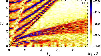
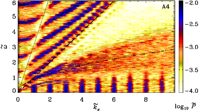
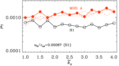
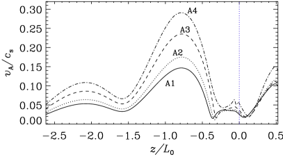
Figure 3: Top: same as top panels in figure 2, but for MHD runs A1 (left) and A4 (right). Bottom left: normalised mode strength $\mu_{f}$ of the $f$-mode as a function of $\widetilde{k}_{x}$ for MHD runs A1–A4 (four overlapping red curves with filled circles for A1) as well as for the hydrodynamic run H1 (open circles; solid black); bottom right: vertical profiles of $v_{\rm A}/c_{\rm s}$ in the saturated state of the background magnetic field for models A1 (solid), A2 (dotted), A3 (dashed) and A4 (dash-dotted). See table 1 for more details.

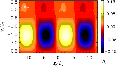
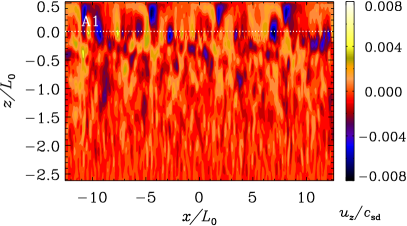
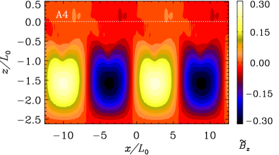
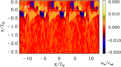
Figure 4: Snapshots of normalised vertical magnetic field $\tilde{B}_{z}=B_{z}/c_{\rm sd}\sqrt{\mu_{0}{\rho_{\rm d}}(0)}$ (left), and $u_{z}/c_{\rm sd}$ (right) in the saturated state of the background magnetic field $\bm{B}_{0}$ for MHD runs A1 (top) and A4 (bottom) shown in the $x$-$z$ plane with dotted horizontal lines marking the location of the interface at $z=0$.

Here we investigate the effects of harmonically varying subsurface magnetic fields, maintained by the EMF ${\cal E}_{0y}^{\rm A}$ as given in equation (6), on the $f$-mode. We refer first to the $k\omega$ diagrams for runs A1 and A4, shown in the top panels of figure 3. The vertical stripes at low frequencies correspond to the unstable Bloch modes, which arise due to the periodicity of the background magnetic field; see Singh et al. (2014). Comparing these $k\omega$ diagrams with the one from the suitable hydrodynamic run H1 (see table 1) shown in figure 2, we see that the $f$-modes in the MHD runs are very different, thus already providing evidence that the $f$-mode is sensitive to subsurface magnetism in our setup. This, in a sense, confirms earlier analytical work, e.g. Roberts (1981), where larger frequencies of the $f$-mode are expected, although the fanning and associated mode strengthening were not anticipated then. Let us define the $z$-dependent rms Alfvén speed, $v_{\rm A}(z)$, as

$$v_{\rm A}(z)=\sqrt{\frac{\langle B^{2}\rangle_{x}(z)}{\mu_{0}\langle\rho\rangle_{x}(z)}}\,,$$ (12)

where $\langle\cdot\rangle_{x}$ denotes averaging along the $x$ direction. The vertical profiles of $v_{\rm A}(z)/c_{\rm s}(z)$ are shown in the bottom right panel of figure 3 for all A runs.

In the bottom left panel of figure 3, we show the wavenumber dependence of the normalised mode strength $\mu_{\rm f}$ of the $f$-mode for the A runs and the corresponding hydrodynamic run H1. All the input parameters for these runs are the same (see table 1), except for the magnetic field strength which is gradually increased from A1 to A4 while keeping its maximum at the same depth; see figure 3. Compared to the run H1, the mode strength is clearly larger in the A runs for all $\widetilde{k}_{x}>1.5$. Interestingly, the mode strength is nearly the same for runs A1–A4, while the line width (or fanning) of the $f$-mode increases from A1 to A4, as can be inferred from the $k\omega$ diagrams. Snapshots of the vertical components $B_{z}$ and $u_{z}$ are shown in figure 4 for models A1 and A4 in the saturated stage of the background magnetic fields, where their maxima lie more than one pressure scale height below the interface at $z=0$. While no large scale flow is noticeable in the weakly magnetised case A1, we do see a systematic flow pattern in model A4 with a stronger magnetic concentration. Despite the appearance of systematic flows in these MHD runs, the normalised $f$-mode strength is found to be nearly the same in all the A runs, as can also be seen from the corresponding values of $\Sigma_{\rm f}$ (identical when rounded to three decimal places) listed in table 1.

3.3 MHD B-type runs

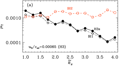
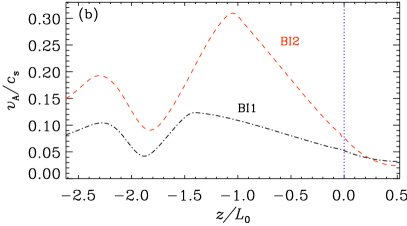
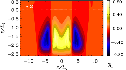
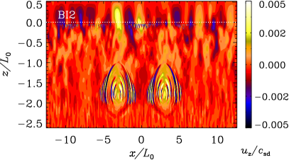
Figure 5: Top: (a) normalised mode strength $\mu_{f}$ of the $f$-mode as a function of $\widetilde{k}_{x}$ for MHD B-runs BI1 (diamonds; dash-dotted black) and BI2 (open circles; dashed red) as well as for the appropriate hydrodynamic run H3 (filled circles; solid black), and (b) vertical profiles of $v_{\rm A}/c_{\rm s}$ in the saturated state of the background magnetic field for the corresponding MHD cases, shown in left and right panels, respectively. Bottom: same as top panels in figure 4 but for the run BI2. See table 1 for more details.

Next we turn to MHD B-type models, where localised magnetic concentrations are maintained below the surface by the EMF ${\cal E}_{0y}^{\rm B}$, as given in equation (7). Their horizontal extent $\Delta x_{B}=x_{2}-x_{1}$ is thus restricted, with $\Delta\tilde{x}_{B}\approx 4\pi$ (i.e., half the horizontal extent of the domain) for the two BI-type models BI1 and BI2 and $\Delta\tilde{x}_{B}\approx 7\pi$ for model BII; see the bottom left panels of figures 5 and 6, and table 1 for details.

The $k\omega$ diagrams for models BI2 and BII are shown in figure 7. Remarkably, the unstable Bloch modes seen as vertical stripes at low frequencies in the A-type runs are completely absent here. These were first found in Singh et al. (2014) and thought to arise due to the periodicity of the background magnetic field (Berton & Heyvaerts, 1987). Given that the appearance of solar ARs during most phases of the magnetic activity cycle is hardly ever periodic in longitude, the Bloch modes are unlikely to be seen. Yet, during very active phases of the Sun, these modes are potentially observable in the $k\omega$ or ring diagrams that are constructed from sufficiently large patches covering many ARs which show a regular pattern of alternating positive and negative vertical magnetic field along the azimuthal direction. On the other hand, given the drastic difference between our A- and B-type runs, we must acknowledge that the Bloch modes are rather sensitive to the exact matching of the wavelength and the size of the patch. This limits the observability of Bloch modes severely.

As for models A1–A4, a direct comparison of diagnostic diagrams shown in figures 2 and 7 reveals that the $f$-mode is significantly perturbed in the presence of subsurface magnetic fields; compare, e.g., BI2 with the corresponding hydrodynamic case H3 where the hydrodynamic forcing is restricted to $\tilde{z}<0$ (see also table 1). The $f$-mode in the MHD run BI2 appears to exist at all wavenumbers shown, whereas it is markedly damped at large wavenumbers in the corresponding hydrodynamic run H3. Moreover, the fanning of the $f$-mode, as discussed above (see also Singh et al., 2014), is much weaker here for localised magnetic field concentrations.

The wavenumber dependence of $\mu_{\rm f}$ for the two BI-runs and the relevant hydrodynamic run H3, as well as the vertical profiles of the normalised Alfvén speed for these MHD runs are shown in the top panels of figure 5. For a meaningful comparison, the $f$-mode strengths were determined from data sets with identical time-spans, which can, in general, affect the mode strengths. The label H3s, used in figure 5(a) signifies that the data are from run H3, but $\mu_{\rm f}$ is determined from a shorter time-series, matching the ones in BI1 and BI2.

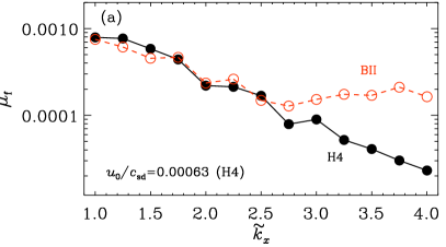
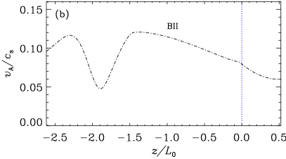
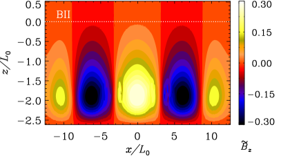
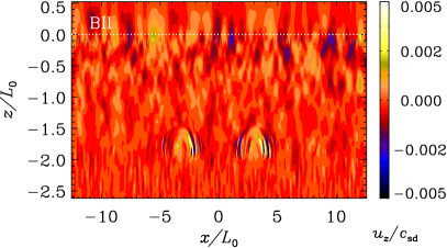
Figure 6: Same as figure 5 but for the MHD run BII; see table 1 for more details.

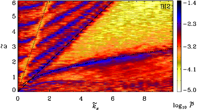
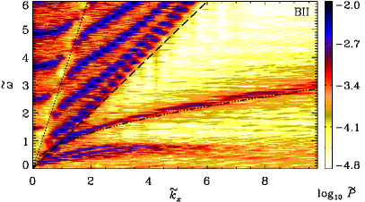
Figure 7: $k\omega$ diagrams for MHD B-type runs BI2 (left) and BII (right); see table 1 for more details.

From figure 5(a) we see that $\mu_{\rm f}$ for the MHD run BI1 with weak magnetic concentration is nearly the same as in case of run H3s. Note also that the maximum of the Alfvén-to-sound speed ratio in this case lies at a larger depth compared to the A runs; see figure 5(b) and table 1. This may be another reason why we do not find mode strengthening in BI1. However, when the magnetic field is increased and its maximum moves upwards to somewhat shallower depths as in case of BI2, we immediately find the $f$-mode strengthening at wavenumbers $\widetilde{k}_{x}\geq 1.8$. Snapshots of $B_{z}$ and $u_{z}$ are shown in the bottom panels of figure 5 for model BI2. The horizontal oscillations in $u_{z}$ in the proximity of regions of strong magnetic field may seem to be numerical artifacts, but they do not look like the regular “ringing” one encounters when a simulation is underresolved. As they are resolved by a few mesh points per period, they may well be real. Comparing these with the relevant hydrodynamic run H3 (see figure 2) we find that the vertical motions are comparable and have no large scale feature at the interface. As expected, a systematic flow pattern is indeed seen in deeper layers around the maximum of the magnetic concentration, but, as was argued before based on the A runs, it is not clear whether such flows can affect the mode strength of the $f$-mode which is determined from vertical motions only at the interface.

In those of our experiments where the forcing is further restricted to layers $\tilde{z}<-0.2$, as in the MHD model BII or in the hydrodynamic run H4 (see table 1), we still find evidence of $f$-mode strengthening in the presence of subsurface magnetic fields, but at larger wavenumbers (in this case for $\widetilde{k}_{x}\geq 2.5$). This is demonstrated in figure 6, where snapshots of $B_{z}$ and $u_{z}$ are also shown. In both models, $\mu_{\rm f}$ first decreases with $\widetilde{k}_{x}$, and, while it saturates at a constant level beyond about $2.5$ in case of BII, it shows a monotonic decrement in H4; see figure 6(a). Interestingly, the $f$-mode strengthening is thus discernible in model BII, but is not present in model BI1, although both have similar magnetic field concentrations at nearly the same depth; see table 1, and compare panel (b) of figures 5 and 6. This is likely due to the larger horizontal extent of the magnetic structure in the case of BII as compared to BI1.

Understanding the exact physical mechanism, responsible for the strengthening of the $f$-mode observed here, is beyond the scope of the present paper. Both the imposed magnetic field and the systematic flow driven by it, can, in principle, influence frequency and strength of the $f$ mode. For assessing the relative importance of these two factors in our studies, let us compare Runs H1 and A1. As can be seen from the upper right panel of figure 4, the systematic flow can hardly be seen near the interface, mostly because of the magnetic field being weak in case A1. So we might conclude that the considerable increase in the relative mode amplitude $\Sigma_{f}$ is mainly due to the magnetic field. By contrast, Run A4 (figure 4, lower right panel) exhibits a systematic flow pattern dominating over the random component of the flow. Hence, it cannot be decided to what extent the systematic flow is affecting $\Sigma_{f}$. In Runs A1-A4, $\Sigma_{f}$ is nearly the same, although the magnetic field is changing by a factor of two. As the magnetic field alone seems to strengthen the $f$ mode, this could be an indication of a counteracting effect of the systematic flow, which grows with the magnetic field, too. More work is needed to understand the role of a systematic or mean flow component on the strength of the $f$-mode. This will be the focus of a separate investigation.

4 Conclusions

We have shown numerically that the $f$-mode is significantly perturbed in the presence of subsurface magnetic fields concentrated one to a few scale heights below the photosphere. The fanning (or increase in line width) of the $f$-mode was first reported in Singh et al. (2014) based on harmonically varying magnetic fields, but the associated mode strengthening was not emphasised there. Here we extended this by also investigating the effects of localised bipolar magnetic fields, resembling more realistically the active region precursors. The fanning effect of the $f$-mode is found to be weaker in the case of localised magnetic field concentrations. Motivated by the observational findings of Singh et al. (2016), where the strengthening at large wavenumbers of the $f$-mode prior to the emergence of about half a dozen active regions, we focus here primarily on the phenomenon of $f$-mode strengthening. In our numerical investigations reported here, the $f$-mode strength is found to be clearly larger at high horizontal wavenumbers in a variety of magnetic background states, compared to their corresponding hydrodynamic cases. While the fanning of the $f$-mode at large $k_{x}$ is more sensitive to the strength of the magnetic field at a given depth, the mode strength itself shows a dependence on the location of the magnetic concentration beneath the surface. Thus, it is indeed remarkable that the properties of the $f$-mode trace so effectively both the location and the strength of subsurface magnetic fields that are not yet directly visible at the photosphere.

We note that damping of the $f$-mode due to its resonant coupling with atmospheric magnetic fields or due to absorption caused by sunspots is known (Cally & Bogdan, 1997; Erdélyi, 2006; Pintér et al., 2007), and also seen in observational studies of Singh et al. (2016) after the emergence of active regions. But, the strengthening of the $f$-mode due to magnetic fields confined below the photosphere is a qualitatively different finding, which is numerically confirmed in the present work.

Let us now estimate the instrumental requirements to robustly probe and detect solar $f$-mode perturbations of the kind explored in this paper. In order to detect both fanning and mode-strength gain, according to figures 3 and 5, $\widetilde{k}_{x}\gtrsim 2$ needs to be reached. With $\gamma H_{\rm d}\approx 0.5\,{\rm Mm}$ and $R_{\odot}=700\,{\rm Mm}$ being the solar radius, this corresponds to spherical harmonic degrees $\ell\gtrsim 2800$. However, indications of $f$-mode strengthening prior to active region formation could indeed be available even at somewhat smaller degrees, as was seen in the observational work of Singh et al. (2016) based on data from the HMI instrument, whose sensitivity drops beyond $\ell\approx 2000$. The precursor signal is expected to improve at larger wavenumbers and therefore higher resolution data from other facilities and upcoming missions will be critical not only for establishing the connection between the solar $f$-mode and the subsurface magnetic fields, but also for providing deeper insights into the sunspot formation mechanism, which is still an outstanding topic in solar physics. More work is needed to understand the physical mechanism responsible for such a strengthening of the $f$-mode and this will be attempted elsewhere. In particular, it would be useful to extend these models to explore effects of 3-dimensional magnetic configurations; see the review of Erdélyi (2006) for possible effects on mode damping and mode conversion.

References

- Barnes et al. (2014) Barnes, G., Birch, A. C., Leka, K. D., & Braun, D. C., “Helioseismology of Pre-emerging Active Regions. III. Statistical Analysis,” Astrophys. J. 786, 19 (2014).
- Basu (2016) Basu, S., “Global seismology of the Sun,” Liv. Rev. Solar Phys. 13, 2 (2016).
- Berton & Heyvaerts (1987) Berton, R., & Heyvaerts, J., “Magnetohydrodynamic modes of a periodic magnetic medium,” Solar Phys. 109, 201–231 (1987).
- Birch et al. (2013) Birch, A. C., Braun, D. C., Leka, K. D., Barnes, G., & Javornik, B., “Helioseismology of Pre-emerging Active Regions. II. Average Emergence Properties,” Astrophys. J. 762, 131 (2013).
- Brandenburg (2001) Brandenburg, A., “The inverse cascade and nonlinear alpha-effect in simulations of isotropic helical hydromagnetic turbulence,” Astrophys. J. 550, 824–840 (2001).
- Brandenburg (2005) Brandenburg, A., “The case for a distributed solar dynamo shaped by near-surface shear,” Astrophys. J. 625, 539–547 (2005).
- Brandenburg et al. (2016) Brandenburg, A., Rogachevskii, I., & Kleeorin, N., “Magnetic concentrations in stratified turbulence: the negative effective magnetic pressure instability,” New J. Phys. 18, 125011 (2016).
- Cally & Bogdan (1993) Cally, P. S., & Bogdan, T. J., “Solar p-modes in a vertical magnetic field - Trapped and damped pi-modes,” Astrophys. J. 402, 721–732 (1993).
- Cally & Bogdan (1997) Cally, P. S., & Bogdan, T. J., “Simulation of f- and p-Mode interactions with a stratified magnetic field concentration,” Astrophys. J. Lett. 486, L67–L70 (1997).
- Cally et al. (1994) Cally, P. S., Bogdan, T. J., & Zweibel, E. G., “Umbral oscillations in sunspots: Absorption of p-modes and active region heating by mode conversion,” Astrophys. J. 437, 505–521 (1994).
- Campos (2011) Campos, L. M. B. C.,, “On magnetoacoustic-gravity-inertial (MAGI) waves - I. Generation, propagation, dissipation and radiation,” Month. Not. Roy. Astron. Soc. 410, 717–734 (2011).
- Chandrasekhar (1961) Chandrasekhar, S. Hydrodynamic and Hydromagnetic Stability. Dover Publications, New York (1961).
- Charbonneau (2010) Charbonneau, P., “Dynamo models of the solar cycle,” Liv. Rev. Solar Phys. 7, 3 (2010).
- Christensen-Dalsgaard (2003) Christensen-Dalsgaard, J., 2003, Lecture notes on stellar oscillations, 5th edition, http://users-phys.au.dk/jcd/oscilnotes/
- Daiffallah et al. (2011) Daiffallah, K., Abdelatif, T., Bendib, A., Cameron, R., & Gizon, L., “3D Numerical Simulations of f-Mode Propagation Through Magnetic Flux Tubes,” Solar Phys. 268, 309–320 (2011).
- Erdélyi (2006) Erdélyi, R., “Magnetic coupling of waves and oscillations in the lower solar atmosphere: can the tail wag the dog?,” Roy. Soc. of Lon. Tran. Ser. A 364, 351–381 (2006).
- Felipe et al. (2012) Felipe, T., Braun, D., Crouch, A., & Birch, A., “Scattering of the f-mode by Small Magnetic Flux Elements from Observations and Numerical Simulations,” Astrophys. J. 757, 148 (2012).
- Felipe et al. (2013) Felipe, T., Crouch, A., & Birch, A., “Numerical simulations of multiple scattering of the -mode by flux tubes,” Astrophys. J. 775, 74 (2013).
- Fernandes et al. (1992) Fernandes, D. N., Scherrer, P. H., Tarbell, T. D., & Title, A. M., “Observations of high-frequency and high-wavenumber solar oscillations,” Astrophys. J. 392, 736–738 (1992).
- Gough (1987) Gough, D. O., “Lectures on Linear adiabatic stellar pulsation,” In Astrophysical fluid dynamics (ed. J.-P. Zahn & J. Zinn-Justin), pp. 399–560. North-Holland, Amsterdam (1987).
- Hanasoge et al. (2008) Hanasoge, S. M., Birch, A. C., Bogdan, T. J., & Gizon, L., “-mode interactions with thin flux tubes: the scattering matrix,” Astrophys. J. 680, 774–780 (2008).
- Hanasoge et al. (2016) Hanasoge, S. M., Gizon, L., & Sreenivasan, K. R., “Seismic sounding of convection in the Sun,” Ann. Rev. Fluid Dyn. 48, 191–217 (2016).
- Hartlep et al. (2011) Hartlep, T., Kosovichev, A. G., Zhao, J., & Mansour, N. N., “Signatures of Emerging Subsurface Structures in Acoustic Power Maps of the Sun,” Solar Phys. 268, 321–327 (2011).
- Ilonidis et al. (2011) Ilonidis, S., Zhao, J., & Kosovichev, A., “Detection of emerging sunspot regions in the solar interior,” Science 333, 993–996 (2011).
- Käpylä et al. (2012) Käpylä, P. J., Mantere, M. J., & Brandenburg, A., “Cyclic magnetic activity due to turbulent convection in spherical wedge geometry,” Astrophys. J. Lett. 755, L22 (2012).
- Käpylä et al. (2016) Käpylä, P. J., Brandenburg, A., Kleeorin, N., Käpylä, M. J., & Rogachevskii, I., “Magnetic flux concentrations from turbulent stratified convection,” Astron. Astrophys. 588, A150 (2016).
- Khlystova & Toriumi (2017) Khlystova, A., & Toriumi, S., “Photospheric velocity structures during the emergence of small active regions on the Sun,” Astrophys. J. 839, 63 (2017).
- Komm et al. (2008) Komm, R., Morita, S., Howe, R., Hill, F., “Emerging Active Regions Studied with Ring-Diagram Analysis,” Astrophys. J. 672, 1254–1265 (2008).
- Libbrecht et al. (1990) Libbrecht, K. G., Woodard, M. F., & Kaufman, J. M., “Frequencies of solar oscillations,” Astrophys. J. Suppl. 74, 1129–1149 (1990).
- Mȩdrek et al. (1999) Mȩdrek, M., Murawski, K., & Roberts, B., “Damping and frequency reduction of the f-mode due to turbulent motion in the solar convection zone,” Astron. Astrophys. 349, 312–316 (1999).
- Miles & Roberts (1989) Miles, A. J., & Roberts, B., “On the properties of magnetoacoustic surface waves,” Solar Phys. 119, 257–278 (1989).
- Miles & Roberts (1992) Miles, A. J., & Roberts, B., “Magnetoacoustic-gravity surface waves. I - Constant Alfven speed,” Solar Phys. 141, 205–234 (1992).
- Miles et al. (1992) Miles, A. J., Allen, H. R., & Roberts, B., “Magnetoacoustic-gravity surface waves. II - Uniform magnetic field,” Solar Phys. 141, 235–251 (1992).
- Mole et al. (2008) Mole, N., Kerekes, A., & Erdélyi, R., “Effects of Random Flows on the Solar f Mode: I. Horizontal Flow,” Solar Phys. 251, 453–468 (2008).
- Murawski (2000a) Murawski, K., “Influence of Coherent and Random Flows on the Solar F-Mode,” Astrophys. J. 537, 495–502 (2000a).
- Murawski (2000b) Murawski, K., “Turbulent f-mode in a stratified solar atmosphere,” Astron. Astrophys. 360, 707–714 (2000b).
- Murawski & Roberts (1993a) Murawski, K. and Roberts, B., “Random velocity field corrections of the f-mode. I. Horizontal flows,” Astron. Astrophys. 272, 595– (1993a).
- Murawski & Roberts (1993b) Murawski, K. and Roberts, B., “Random velocity field corrections of the f-mode. II. Vertical and horizontal flow,” Astron. Astrophys. 272, 601– (1993b).
- Parchevsky & Kosovichev (2009) Parchevsky, K. V., & Kosovichev, A. G., “Numerical Simulation of Excitation and Propagation of Helioseismic MHD Waves: Effects of Inclined Magnetic Field,” Astrophys. J. 694, 573–581 (2009).
- Pintér (2008) Pintér, B., “Modelling the Coupling Role of Magnetic Fields in Helioseismology,” Solar Phys. 251, 329–340 (2008).
- Pintér & Erdélyi (2018) Pintér, B. and Erdélyi, R., “Fundamental (f) oscillations in a magnetically coupled solar interior-atmosphere system – an analytical approach,” Adv. Space Res. 61, 759–776 (2018).
- Pintér et al. (2007) Pintér, B., Erdélyi, R., & Goossens, M., “Global oscillations in a magnetic solar model. II. Oblique propagation,” Solar Phys. 466, 377–388 (2007).
- Roberts (1981) Roberts, B., “Wave propagation in a magnetically structured atmosphere. I - Surface waves at a magnetic interface.,” Solar Phys. 69, 27–38 (1981).
- Schunker et al. (2011) Schunker, H., Cameron, R. H., Gizon, L., & Moradi, H., “Constructing and characterising solar structure models for computational helioseismology,” Solar Phys. 271, 1–26 (2011).
- Singh et al. (2014) Singh, N. K., Brandenburg, A., & Rheinhardt, M., “Fanning out of the solar -mode in presence of nonuniform magnetic fields?” Astrophys. J. Lett. 795, L8 (2014).
- Singh et al. (2015) Singh, N. K., Brandenburg, A., Chitre, S. M., & Rheinhardt, M., “Properties of - and -modes in hydromagnetic turbulence,” Month. Not. Roy. Astron. Soc. 447, 3708–3722 (2015).
- Singh et al. (2016) Singh, N. K., Raichur, H., & Brandenburg, A., “High-wavenumber solar -mode strengthening prior to active region formation,” Astrophys. J. 832, 120 (2016).
- Thomas (1983) Thomas, J. H., “Magneto-atmospheric waves,” Ann. Rev. Fluid Mech. 15, 321–343 (1983).
- Thompson (2006) Thompson, M. J., “Magnetohelioseismology,” Roy. Soc. of Lon. Tran. Ser. A 364, 297–311 (2006).