Discovery of Strongly Inverted Metallicity Gradients in Dwarf Galaxies at $z$$\sim$2

Abstract

We report the first sub-kiloparsec spatial resolution measurements of strongly inverted gas-phase metallicity gradients in two dwarf galaxies at $z$$\sim$2. The galaxies have stellar masses $\sim$$10^{9}$$M_{\odot}$, specific star-formation rate $\sim$20 $\rm Gyr$ ^-1, and global metallicity $12+\log({\rm O/H})\sim 8.1$ (1/4 solar), assuming the Maiolino et al. (2008) strong line calibrations of [O iii]/H$\beta$ and [O ii]/H$\beta$. Their metallicity radial gradients are measured to be highly inverted, i.e., 0.122$\pm$0.008 and 0.111$\pm$0.017 dex/kpc, which is hitherto unseen at such small masses in similar redshift ranges. From the Hubble Space Telescope observations of the source nebular emission and stellar continuum, we present the 2-dimensional spatial maps of star-formation rate surface density, stellar population age, and gas fraction, which show that our galaxies are currently undergoing rapid mass assembly via disk inside-out growth. More importantly, using a simple chemical evolution model, we find that the gas fractions for different metallicity regions cannot be explained by pure gas accretion. Our spatially resolved analysis based on a more advanced gas regulator model results in a spatial map of net gaseous outflows, triggered by active central starbursts, that potentially play a significant role in shaping the spatial distribution of metallicity by effectively transporting stellar nucleosynthesis yields outwards. The relation between wind mass loading factors and stellar surface densities measured in different regions of our galaxies shows that a single type of wind mechanism, driven by either energy or momentum conservation, cannot explain the entire galaxy. These sources present a unique constraint on the effects of gas flows on the early phase of disk growth from the perspective of spatially resolved chemical evolution within individual systems.

1. Introduction

Galaxy formation models require inflows and outflows of gas to regulate star formation (Finlator & Davé, 2008; Recchi et al., 2008; Bouche et al., 2010; Davé et al., 2012; Dayal et al., 2013; Dekel et al., 2013; Lilly et al., 2013; Dekel & Mandelker, 2014; Peng & Maiolino, 2014; Pipino et al., 2014), yet this “baryon cycle” is not quantitatively understood. The interstellar medium (ISM) oxygen abundance (i.e. metallicity) and its spatial distribution is fortunately a key observational probe of this process (Tremonti et al., 2004; Erb et al., 2006; Maiolino et al., 2008; Bresolin et al., 2009; Mannucci et al., 2010, 2011; Zahid et al., 2011; Yates et al., 2012; Zahid et al., 2012; Henry et al., 2013a; Jones et al., 2013; Sanchez et al., 2014; Zahid et al., 2014; Bresolin & Kennicutt, 2015; Ho et al., 2015; Sanders et al., 2015; Strom et al., 2016). “Inside-out” galaxy growth implies that initially steep radial gradients of metallicity flatten at later times (higher masses) as disks grow larger, yet other scenarios suggest metallicities are initially well mixed by strong galactic feedback, and then locked into negative gradients as winds lose the power to disrupt massive gas disks (Prantzos & Boissier, 2000; Hou et al., 2000; Mollá & Díaz, 2005; Kobayashi & Nakasato, 2011; Few et al., 2012; Pilkington et al., 2012; Gibson et al., 2013; Ma et al., 2017). What in common between these scenarios is that none of them predict the existence of a steep positive (i.e. inverted) radial gradient such that metallicity increases with galacto-centric radius.

However, there is growing evidence of such phenomenon in both the local and distant Universe (Cresci et al., 2010; Queyrel et al., 2012; Stott et al., 2014; Troncoso et al., 2014; Sanchez et al., 2014; Pérez-Montero et al., 2016; Wuyts et al., 2016; Belfiore et al., 2017; Carton et al., 2018). The key reason for local galaxies possessing inverted gradients is gas re-distribution by tidal force in strongly interacting systems (Kewley et al., 2006, 2010; Rupke et al., 2010; Rich et al., 2012; Torrey et al., 2012). At high redshifts, inverted gradients are often attributed to the inflows of metal-poor gas from the filaments of cosmic web, infalling directly onto galaxy centers, diluting central metallicities and hence creating positive gradients (Cresci et al., 2010; Mott et al., 2013). Given most of the high-$z$ observations are conducted from the ground with natural seeing, the targets are usually super-$L_{\ast}$ galaxies with stellar mass ($M_{\ast}$) $\gtrsim$$10^{10}$$M_{\odot}$ (see e.g., Troncoso et al., 2014).

These high-$z$ inverted gradients are in concert with the “cold-mode” gas accretion which has long been recognized to play a crucial role in galaxies getting their baryonic mass supply (Birnboim & Dekel, 2003; Kereš et al., 2005; Dekel & Birnboim, 2006; Dekel et al., 2009b; Kereš et al., 2009). Instead of being shock-heated to dark matter (DM) halo virial temperature ($\sim$10⁶K for a $M_{\rm h}$$\sim$10¹²$M_{\odot}$ halo) and then radiate away the thermal energy to condense and form stars (vis-á-vis “hot-mode” accretion), gas streams can remain relatively cold (<10⁵K) while being steadily accreted onto galaxy disks. This cold accretion dominates the growth of galaxies forming in low-mass halos irrespective of redshifts since a hot permeating halo of virialized gas can only manifest in halos above 2-3$\times 10^{11}$$M_{\odot}$, at $z\lesssim 2$ (Birnboim & Dekel, 2003; Kereš et al., 2005).

A question thus arises: if cold-mode gas accretion dominates in low-mass systems (with $M_{\ast}$ less than a few $10^{10}$$M_{\odot}$) and is thought to lead to inverted gradients under the condition that the incoming gas streams are centrally directed, can we observe this phenomenon in dwarf galaxies (with $M_{\ast}\lesssim 10^{9}$) at high redshifts? The answer is not straightforward since the effect of ejective feedback (e.g. galactic winds driven by supernovae) is more pronounced in lower mass galaxies, given their shallower gravitational potential wells and higher specific star-formation rate (sSFR) (see e.g. Hopkins et al., 2014; Vogelsberger et al., 2014). On one hand, galactic winds can bring about kinematic turbulence that prevents a smooth accretion of filamentary gas streams directly onto galaxy center, resulting in rapid formation of in-situ clumps (Dekel et al., 2009a). On the other hand, metal-enriched outflows triggered by these powerful winds can help remove stellar nucleosynthesis yields from galaxy center (Tremonti et al., 2004; Erb et al., 2006). Therefore the existence of strongly inverted gradients in dwarf galaxies at high redshifts, if any, presents a sensitive test of the relative strength of feedback-induced radial gas flows, in the early phase of the disk mass assembly process. There have not been any attempts to investigate such existence, primarily due to the small sizes of these dwarf galaxies and sub-kiloparsec (sub-kpc) spatial resolution required to yield accurate gradient measurements (Yuan et al., 2013). In this work, we present the first effort to secure two robustly measured inverted metallicity gradients in $z\sim 2$ star-forming dwarf galaxies from the Hubble Space Telescope (HST) near-infrared (NIR) grism slitless spectroscopy, aided with galaxy cluster lensing magnification. The details of data and sample galaxies are presented in Section 2. We describe our analysis methods alongside main results in Section 3, and conclude in Section 4. Throughout this paper, a flat $\Lambda$CDM cosmology ($\Omega_{\rm{m}}$ =0.3, $\Omega_{\Lambda}$ =0.7, $H_{0}$=70$\rm km\leavevmode\nobreak\ s^{-1}\leavevmode\nobreak\ Mpc^{-1}$) is assumed.

2. Data and galaxy sample

The two galaxies with exceptional inverted gradients are selected from a comprehensive study of $\sim$300 galaxies with metallicity measurements at $1.2\lesssim z\lesssim 2.3$ (Wang et al. 2017; Wang et al. in prep.). Before we discuss the two systems in detail in Section 2.4, we give for convenience a brief summary of the spectroscopic data (Section 2.1), a concise description of the data reduction procedure (Section 2.2), and the ancillary imaging used in this work (Section 2.3).

2.1. HST grism slitless spectroscopy

We use the diffraction-limited spatially resolved slitless spectroscopy, obtained using the HST wide-field camera 3 (WFC3) NIR grisms (G102 and G141), acquired by the Grism Lens-Amplified Survey from Space (GLASS, Schmidt et al., 2014; Treu et al., 2015). GLASS observes the distant Universe through 10 massive galaxy clusters as natural telescopes, exposing 10 orbits of G102 (0.8-1.15$\mu\textrm{m}$, $R$$\sim$210) and 4 orbits of G141 (1.1-1.7$\mu\textrm{m}$, $R$$\sim$130) per sightline. This amounts to a sum of $\sim$22 kiloseconds of G102 and $\sim$9 kiloseconds of G141, as well as $\sim$7 kiloseconds of F140W+F105W direct imaging for astrometric alignment and wavelength/flux calibrations per field. These exposures distributed over two separate pointings per cluster with nearly orthogonal orientations, designed to help disentangle spectral contamination from neighboring objects. So for each source, two sets of G102+G141 spectrum are obtained, covering an uninterrupted wavelength range of 0.8-1.7$\mu\textrm{m}$ with almost unchanging sensitivity, reaching a 1-$\sigma$ surface brightness of $3\times 10^{-16}\leavevmode\nobreak\ \rm erg\leavevmode\nobreak\ s^{-1}\leavevmode\nobreak\ cm^{-2}\leavevmode\nobreak\ arcsec^{-2}$ across the entire spectral range. The GLASS collaboration has made the catalogs of their redshift identifications in the 10 fields, based on visual inspections of emission line (EL) features, publicly available at https://archive.stsci.edu/prepds/glass/.

2.2. Grism data reduction

To explore the chemical properties of galaxies at the peak epoch of cosmic chemical enrichment, we select from these catalogs, a parent sample consisting of $\sim$300 galaxies with secure redshifts (i.e. redshift quality $\geq$3 in the publicly available catalogs as described by Treu et al. (2015)) in the range of $1.2\lesssim z\lesssim 2.3$. This range is chosen for the detection of multiple nebular ELs — in particular the Balmer lines, [O iii], and [O ii]— enabling the metallicity measurements, as in our earlier work (Jones et al., 2015b; Wang et al., 2017). The GLASS data for these $\sim$300 galaxies are reduced using the Grism Redshift and Line analysis (Grzili ; G. Brammer et al. in prep) software. Grzili presents an end-to-end processing of the paired grism and direct exposures. The procedure includes five steps: 1) pre-processing of the raw grism exposures, 2) full field-of-view (FoV) grism model construction, 3) 1D/2D spectrum extraction, and 4) solving for best-fit redshift from spectral template fitting (see Appendix A for more details), 5) refining full FoV grism model and extractions of source 1D/2D spectrum and EL stamps. In step 1), the pre-processing consists of hot-pixel/persistence masking, cosmic ray flagging, flat fielding, astrometric alignment, sky background subtraction, and extraction of visit-level source catalogs and segmentation maps. In step 5), the EL stamps are drizzled onto a grid with a pixel scale of $0\farcs 06$, Nyquist sampling the WFC3 point spread function (PSF). We apply an additional step on the Grzili output products to obtain pure 2D maps of [O iii] $\lambda$5008 and H$\beta$, clean from the partial contamination of [O iii] $\lambda$4960, due to the limited grism spectral resolution and extended source morphology. Our procedure properly combines EL maps at multiple orientations, preserving angular resolution and accounting for EL blending.

2.3. HST imaging: estimating $M_{\ast}$ from SED fitting

In addition to the deep NIR spectroscopy, there exists a wealth of ancillary imaging data with equally high spatial resolution on the 10 GLASS fields, which encompass all 6 Hubble Frontier Field (HFF, Lotz et al., 2016) clusters and 4 from the Cluster Lensing And Supernova Survey with Hubble (CLASH, Postman et al., 2012). These broad-band photometry, covering observed wavelengths of $\sim$0.4-1.7 $\mu\textrm{m}$, can help constrain stellar population properties (especially $M_{\ast}$) of our selected $\sim$300 galaxies at sufficient confidence. We use the images sampled with $0\farcs 06$ pixel size, and apply kernel convolutions to match the angular resolution of all images to that of the F160W filter. We subtract contamination from intracluster light using established procedures (Morishita et al., 2016). Since our targets have rest-frame optical ELs with high equivalent widths (EWs), we subtract the nebular flux contribution from the broad-band photometry to obtain the stellar continuum flux. As given in Appendix A, we model the nebular ELs as Gaussian profiles centered at the corresponding wavelengths. The nebular contribution to the broad-band photometry is thereby estimated by convolving the filter throughput with the best-fit Gaussian profiles, and then subtracted off. We then fit the stellar continuum spectral energy distribution (SED) with the Bruzual & Charlot (2003) (BC03) stellar population synthesis models using the software FAST (Kriek et al., 2009). We assume a Chabrier (2003) initial mass function (IMF), constant star formation history, stellar dust attenuation in the range $A_{\rm V}^{\rm S}$=0-4 with a Calzetti et al. (2000) extinction curve, and age ranging from 5 Myr to the Hubble time at the redshifts of our targets. Stellar metallicity is fixed to 1/5 solar and we verify that this assumption affects the results by no more than <0.05 dex on $M_{\ast}$.

2.4. Two dwarf galaxies with strongly inverted metallicity gradients

Out of the parent sample of $\sim$300 galaxies, we are able to secure accurate (i.e. at sub-kpc resolution) radial metallicity gradients on 81 sources with suitable spatial extent and high signal-to-noise ratio (SNR) nebular emission. These extended sources typically have half-light radii $R_{50}\gtrsim 0\farcs 15$. In a range of $7\lesssim\log\left(M_{\ast}/M_{\odot}\right)\lesssim 10$ given by the analyses in Section 2.3, our sample probes much lower $M_{\ast}$ than other surveys of spatially resolved line emission at similar redshifts (Wuyts et al., 2016; Förster Schreiber et al., 2018), thanks to the enhanced resolution from lensing magnification, and high sensitivity of the HST NIR grisms. We have previously described the properties of 10 galaxies in our sample from the cluster MACS1149.6+2223 (Wang et al., 2017); results for the full sample are in preparation.

In most cases, we find that metallicity gradients are approximately flat (i.e. consistent with zero given the typical $\sigma=0.03$ dex kpc^-1) or slightly negative. A minority (10/81) of our sample shows positive (i.e. “inverted”) gradients, which are of interest as they pose a challenge to standard galactic chemical evolution models (e.g., Mollá & Díaz, 2005). We have selected the two best examples with strongly inverted gradients for further study in this paper. The two sources are ID03751 ($z=1.96,\leavevmode\nobreak\ M_{\ast}=1.12\times 10^{9}M_{\odot}$) in the prime field of Abell 370, and ID01203 ($z=1.65,\leavevmode\nobreak\ M_{\ast}=2.55\times 10^{9}M_{\odot}$) in the prime field of MACS0744.9+3927.

Table 1 presents their properties. Figure 1 shows the color-composite HST images of these two galaxies and their 2D spatially resolved maps of the nebular ELs. Remarkably, they have $M_{\ast}$ considerably lower — by one order of magnitude — than those of previous positive gradients measured at similar redshifts (see e.g., Cresci et al., 2010; Queyrel et al., 2012; Stott et al., 2014; Troncoso et al., 2014). To complement the low dispersion grism spectra, we have obtained adaptive optics (AO) assisted kinematic data on our sources using ground-based integral-field unit (IFU) spectrograph when available. The observation of source ID01203 is presented in Appendix B. The full data analysis is presented in Hirtenstein et al. (2018) in detail.

Table 1Measured quantities of the two dwarf galaxies

ID	03751	01203
cluster	Abell 370	MACS0744.9+3927
R.A. (deg.)	39.977361	116.197585
Decl. (deg.)	-1.591636	39.456698
$z_{\rm spec}$	1.96	1.65
$\mu$	6.35${}_{-0.58}^{+0.40}$	2.25${}_{-0.03}^{+0.04}$
Observed emission line fluxes
$f_{[\textrm{O}\leavevmode\nobreak\ \textsc{iii}]}$ [$10^{-17}$$\rm erg\leavevmode\nobreak\ s^{-1}\leavevmode\nobreak\ cm^{-2}$ ]	111.41$\pm$0.84	117.66$\pm$1.17
$f_{\textrm{H}\beta}$ [$10^{-17}$$\rm erg\leavevmode\nobreak\ s^{-1}\leavevmode\nobreak\ cm^{-2}$ ]	17.68$\pm$0.68	17.46$\pm$1.06
$f_{[\textrm{O}\leavevmode\nobreak\ \textsc{ii}]}$ [$10^{-17}$$\rm erg\leavevmode\nobreak\ s^{-1}\leavevmode\nobreak\ cm^{-2}$ ]	29.57$\pm$0.51	34.00$\pm$0.96
$f_{\textrm{H}\gamma}$ [$10^{-17}$$\rm erg\leavevmode\nobreak\ s^{-1}\leavevmode\nobreak\ cm^{-2}$ ]	7.21$\pm$0.67	7.06$\pm$1.00
Restframe equivalent widths
EW${}_{[\textrm{O}\leavevmode\nobreak\ \textsc{iii}]}$ [Å]	466.22$\pm$3.52	797.14$\pm$7.95
EW${}_{\textrm{H}\beta}$ [Å]	73.98$\pm$2.83	118.29$\pm$7.18
EW${}_{[\textrm{O}\leavevmode\nobreak\ \textsc{ii}]}$ [Å]	79.14$\pm$1.37	123.91$\pm$3.50
EW${}_{\textrm{H}\gamma}$ [Å]	30.18$\pm$2.82	25.73$\pm$3.68
Estimated physical parameters
$M_{\ast}$ [109$M_{\odot}$ ]	1.12${}_{-0.14}^{+0.14}$	2.55${}_{-0.04}^{+0.04}$
$12+\log({\rm O/H})$	8.08${}_{-0.12}^{+0.11}$	8.10${}_{-0.11}^{+0.11}$
$\Delta\log({\rm O/H})/\Delta r$ [dex/kpc]	0.122$\pm$0.008	0.111$\pm$0.017
${\rm SFR}$ [$M_{\odot}\leavevmode\nobreak\ \mathrm{yr}^{-1}$ ]	25.39$\pm$2.19	48.86$\pm$3.04
$A_{\rm V}$	0.84$\pm$0.13	0.90$\pm$0.16
$t_{\rm age}$ [$10^{7}$ yrs]	7.93$\pm$0.88	3.98$\pm$0.51
$M_{\rm gas}$ [109$M_{\odot}$ ]	4.07$\pm$1.27	23.85$\pm$7.33
$f_{\rm gas}$	0.56$\pm$0.24	0.86$\pm$0.35
$B/T$	0.36$\pm$0.14	0.14$\pm$0.07
$R_{\rm eff}$ [kpc]	1.53$\pm$0.12	1.66$\pm$0.17
Gas kinematics
$\sigma$ [km/s]	$\cdots$	73$\pm$3
$V/\sigma$	$\cdots$	1.3$\pm$0.1
Measurements of the gaseous outflows at the central 1$\rm kpc$
$\lambda$	49.9$\pm$14.7	52.1$\pm$20.2
$\Psi$ [$M_{\odot}\leavevmode\nobreak\ \mathrm{yr}^{-1}$ ]	311.3$\pm$96.2	1700.9$\pm$681.9

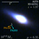
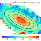
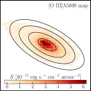
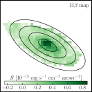
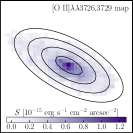
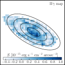
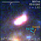
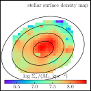
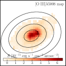
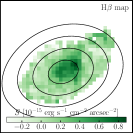
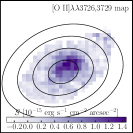
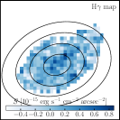
Figure 1.— Two star-forming dwarf galaxies at $z$$\sim$2 displaying unusually strong inverted metallicity gradients, securely determined at sub-kpc spatial resolution. For each source we show, from left to right: color composite image (created from HST broad-band photometry), stellar surface density map (obtained from SED fitting to HST photometry), and surface brightness map of ELs [O iii], H$\beta$, [O ii], and H$\gamma$. The black contours overlaid represent the source plane de-projected galacto-centric radii with 1 kpc interval. The two light-dispersion directions for the grism exposures are denoted by the orange and cyan arrows (see Figures 8 and 9 for the corresponding spectra). The spatial extent and orientation are unchanged for the two sources in all 2D stamps throughout. North is up and east is to the left.

3. Methods and results

In this section, we describe our key methods used to derive radial metallicity gradients (Section 3.1), 2D maps of ${\rm SFR}$, average stellar population age, and gas fraction (Section 3.2), as well as spatial distributions of net gaseous outflow rate and mass loading factor (Section 3.3). The main results are presented alongside the corresponding methods.

3.1. Radial metallicity gradients

Since we infer metallicity from strong line flux ratio diagnostics, calibrated by either empirical methods, or theoretical methods, or a hybrid of both, it is essential to make sure that the line emission is not contaminated by active galactic nucleus (AGN) ionization or shock excitation. As shown in Figure 2, we verify that our targets have a low probability (<%10) of being classified as AGNs according to the mass-excitation diagram (Juneau et al., 2014). Their individual radial annuli also have excitation and ionization states compatible with Hii regions, as revealed in their loci in the “blue” diagnostic diagrams of $f_{[\textrm{O}\leavevmode\nobreak\ \textsc{iii}]}/f_{\textrm{H}\beta}$ versus $f_{[\textrm{O}\leavevmode\nobreak\ \textsc{ii}]}/f_{\textrm{H}\beta}$ (the middle panel of Figure 2) and O₃₂=$(f_{[\textrm{O}\leavevmode\nobreak\ \textsc{iii}]\lambda 5008}+f_{[\textrm{O}\leavevmode\nobreak\ \textsc{iii}]\lambda 4960})/f_{[\textrm{O}\leavevmode\nobreak\ \textsc{ii}]}$ versus R₂₃=$(f_{[\textrm{O}\leavevmode\nobreak\ \textsc{iii}]\lambda 5008}+f_{[\textrm{O}\leavevmode\nobreak\ \textsc{iii}]\lambda 4960}+f_{[\textrm{O}\leavevmode\nobreak\ \textsc{ii}]})/f_{\textrm{H}\beta}$ (the right panel of Figure 2) (Lamareille et al., 2004; Rodrigues et al., 2012; Jones et al., 2015a). Notably, the intrinsic ratios of R₂₃ and O₃₂ decrease with galacto-centric radius for both of our sources, indicative of positive radial gradients of metallicities, opposite the normal trend, which is confirmed with direct metallicity measurements in nearby disk galaxies (see e.g., Bresolin et al., 2009; Berg et al., 2015; Croxall et al., 2015, 2016). In the source ID01203 covered by our follow-up OSIRIS observations (see Appendix B), its integrated $f_{[\textrm{N}\leavevmode\nobreak\ \textsc{ii}]}/f_{\textrm{H}\alpha}$ ($\lesssim 0.1$ at 3-$\sigma$) also shows no sign of AGN or shocked gas emission.

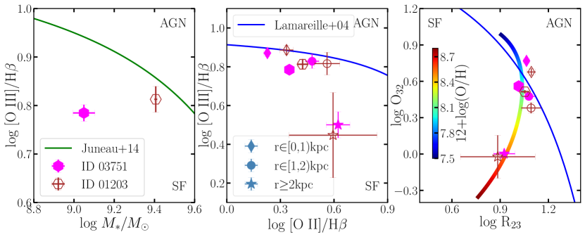
Figure 2.— The diagnostic diagrams for our sources. On the left, we show the mass-excitation diagram with the demarcation scheme between the loci of AGNs and star-forming (SF) galaxies proposed in Juneau et al. (2014). Our galaxies can be safely classified as the latter. In the middle and right panels, we show the “blue” diagrams with the boundaries described by Lamareille et al. (2004). Following the conventions in the left panel, we use filled symbols to represent measurements for ID03751 whilst empty ones for ID01203. Furthermore, the hexagons correspond to the measurements integrated over the entire galaxies (as in the left panel), whereas the other symbols denote results obtained in different radial annuli, as explained in the legend of the middle panel. Again we see that the contamination from AGN ionization is minimum for our sources, even in the central regions. In the right panel, we also show the gas-phase metallicities given by the Maiolino et al. (2008) calibrations involving R₂₃ and O₃₂. The two galaxies presented in this work share similar evolutionary trends in their excitation and ionization states with respect to galacto-centric radius, strongly indicating that their metallicity increases with galacto-centric radius. All the line flux ratios are corrected for dust extinction following the Cardelli et al. (1989) law with nebular attenuation estimated from the observed Balmer decrement of $f_{\textrm{H}\gamma}/f_{\textrm{H}\beta}$ under the assumption of Case B recombination conditions.

Our measurements of radial metallicity gradients largely follow the procedures described in our previous work (Wang et al., 2017). We use a Bayesian approach to jointly infer metallicity ($12+\log({\rm O/H})$), nebular dust extinction ($A_{\rm V}^{\rm N}$), and de-reddened H$\beta$ flux ($f_{\textrm{H}\beta}$). We explore the parameter space using the Markov Chain Monte Carlo sampler Emcee (Foreman-Mackey et al., 2013). The likelihood function is given by $\mathrm{L}\propto\exp(-\chi^{2}/2)$ with

$$\chi^{2}=\sum_{i}\frac{\left(f_{\textrm{EL}_{i}}-R_{i}\cdot f_{\textrm{H}\beta}\right)^{2}}{\left(\sigma_{\textrm{EL}_{i}}\right)^{2}+\left(f_{\textrm{H}\beta}\right)^{2}\cdot\left(\sigma_{R_{i}}\right)^{2}},$$ (1)

where $\textrm{EL}_{i}$ corresponds to each available EL: [O iii], H$\beta$, [O ii], and H$\gamma$. As shown in Figures 8 and 9 in Appendix A, H$\delta$ is only weakly detected for both of our galaxies, with SNR$\lesssim$5 from their spatially integrated grism spectra combined from two orientations, and thereby not included in our Bayesian analysis. On the other hand, our source spectra shows marked detection of the EL $[\textrm{Ne}\leavevmode\nobreak\ \textsc{iii}]\lambda 3869$. However, due to the relatively low wavelength dispersion of the HST NIR grism channels (i.e. $R_{\rm G141}\sim 130$ and $R_{\rm G102}\sim 210$), $[\textrm{Ne}\leavevmode\nobreak\ \textsc{iii}]\lambda 3869$ is heavily blended with He i$\lambda 3889$+H8 on the red side and H9 on the blue side. As a result, we exclude [Ne iii] in our subsequent analyses as well. $f_{\textrm{EL}_{i}}$ and $\sigma_{\textrm{EL}_{i}}$ are the flux and uncertainty of $\textrm{EL}_{i}$. $R_{i}$ is the flux ratio between $\textrm{EL}_{i}$ and H$\beta$, with $\sigma_{R_{i}}$ being the intrinsic scatter at fixed physical properties. In the case $\textrm{EL}_{i}=\textrm{H}\gamma$, $R_{i}$ is given by the Balmer decrement $f_{\textrm{H}\gamma}/f_{\textrm{H}\beta}=0.47$. For $\textrm{EL}_{i}\in\{[\textrm{O}\leavevmode\nobreak\ \textsc{ii}],\leavevmode\nobreak\ [\textrm{O}\leavevmode\nobreak\ \textsc{iii}]\}$, $R_{i}$ and $\sigma_{R_{i}}$ are given by the strong line metallicity diagnostics ($f_{[\textrm{O}\leavevmode\nobreak\ \textsc{iii}]}/f_{\textrm{H}\beta}$ and $f_{[\textrm{O}\leavevmode\nobreak\ \textsc{ii}]}/f_{\textrm{H}\beta}$) calibrated by Maiolino et al. (2008). The Maiolino et al. (2008) calibrations combine the direct electron temperature measurements from the Sloan Digital Sky Survey (SDSS) in the low-metallicity ($12+\log({\rm O/H})$ $\lesssim$ 8.35) branch (Nagao et al., 2006) and the photoionization model predictions in the high-metallicity ($12+\log({\rm O/H})$ $\gtrsim$ 8.35) branch (Kewley & Dopita, 2002), providing a continuous and coherent recipe over a wide metallicity range.

Our metallicity inference presented here primarily originates from the flux ratios between the oxygen collisionally excited lines (CELs) (i.e. [O iii], [O ii]) and H$\beta$ (see the recent review by Maiolino & Mannucci, 2018, for pros and cons of all strong line ratio diagnostics in the literature). Despite their bi-modal relationship with metallicity, R₂₃ and $f_{[\textrm{O}\leavevmode\nobreak\ \textsc{iii}]}/f_{\textrm{H}\beta}$ are found to produce the best accuracy among all the strong line ratios used in $z$$\sim$2 studies (Patrício et al., 2018). Notably, multiple independent analyses have shown that there is a clean metallicity sequence in the diagnostic diagram spanned by $f_{[\textrm{O}\leavevmode\nobreak\ \textsc{iii}]}/f_{\textrm{H}\beta}$ and $f_{[\textrm{O}\leavevmode\nobreak\ \textsc{ii}]}/f_{\textrm{H}\beta}$ (Andrews & Martini, 2013; Jones et al., 2015a; Gebhardt et al., 2015; Curti et al., 2017, also see Figure 2). Since [O iii] and [O ii] are among the brightest and thus most accessible strong ELs in high-$z$ galaxies, the flux ratios involving oxygen CELs will remain the most promising venue for conversion into O/H, since they trace directly the emissivities and abundances of the oxygen ions.

In Appendix C, we perform a comparative study of measuring metallicity gradients with the pure empirical calibrations by Jones et al. (2015a) and Curti et al. (2017), based upon the electron temperature metallicity measurements from the DEEP2 (at $z\sim 0.8$, Newman et al., 2013) and the SDSS (at $0.027<z<0.25$, Abazajian et al., 2009) datasets. We find that the systematic differences between the absolute gradient slopes derived assuming different strong line calibrations can be as high as 0.06 dex/kpc. However, a positive radial gradient slope can always be recovered in each of our sources at high statistical significance, regardless of the calibrations used (see Appendix C for more details). We thus verify that there is no significant bias from the strong line calibrations adopted in our gradient measurements. The same process is applied to both galaxy-integrated fluxes and to fluxes contained in individual spatial pixels (spaxels).

To obtain the correct intrinsic de-projected distance scale for each spaxel, we conducted full source plane morphological reconstruction of our sources. We ray-trace the image of each galaxy to its source plane using up-to-date lens models for each cluster: the macroscopic model of Sharon & Johnson version 4 for Abell 370 (Johnson et al., 2014), and the Zitrin version 2 model for MACS0744.9+3927 (Zitrin et al., 2015). Other lens models are available for these clusters (e.g. Diego et al., 2016; Strait et al., 2018) and we verified that the morphology of each source is robust to the choice of model.

For each source, we fit the SED of individual spaxels using the procedures described in Section 2, obtaining the 2D stellar surface density ($\Sigma_{\ast}$) map shown in Figure 1. Then we reconstruct $\Sigma_{\ast}$ map in the source plane by de-lensing the surface densities according to the deflection field given by the macroscopic lens models. To minimize the stochasticity in stellar population synthesis (Fouesneau & Lançon, 2010; Eldridge, 2012), we make sure that the source plane resolution elements during this reconstruction contain enough stellar masses ($\gtrsim 10^{5}$ $M_{\odot}$) to be representative of complete stellar populations. The axis ratios, inclinations, and major axis orientations are determined from an elliptical Gaussian fit. This procedure provides the intrinsic lensing-corrected morphology, and in particular, the galacto-centric radius at each point of the observed images. The radial scale as black contours in all figures is used to establish the absolute metallicity gradient slope (i.e., in units of dex per proper kpc). From the source reconstructed morphology, we measure their effective radius where the enclosed mass reaches half the total mass of the source. The measurements are represented by $R_{\rm eff}$ in Table 1.

Figure 3 shows the 2D maps of metallicity of our selected two dwarf galaxies at $z\sim 2$. Clearly, the outskirts of our galaxies display highly elevated oxygen abundance ratios. In particular, the outskirts of ID03751 are more metal enriched by $\sim$0.4 dex (i.e. a factor of 2.5) than its center, and more metal-rich by $\sim$0.2 dex than the value inferred based on the fundamental metallicity relation (FMR) given its integrated $M_{\ast}$ Mannucci et al. (2010, 2011). Note that our metallicity measurements extend beyond the source effective radius to cover large enough dynamic range, but not into the region where a plateau/flattening in metallicity (i.e., at $R>2-2.5R_{\rm eff}$, Sanchez et al., 2014; Sánchez-Menguiano et al., 2016) is likely to occur, which might bias the overall gradient determination. For the first time, we are able to detect strongly inverted metallicity gradients in $z$$\sim$2 dwarf galaxies at unprecedentedly high confidence: 0.122$\pm$0.008 dex/kpc for ID03751 ($\sim 15.2\sigma$), and 0.111$\pm$0.017 dex/kpc for ID01203 ($\sim 6.5\sigma$).

The question is thus what caused these dwarf galaxies to have such strongly inverted gradients? First of all, our sources show no evidence of major mergers, supported by their regular morphology displayed in the 2D maps of $M_{\ast}$ and EL surface brightness in Figure 1. For source ID01203 with OSIRIS data, this statement is further strengthened by the kinematic evidence of disk orderly rotation. Secondly, the fact that the outskirts of our sources show elevated metallicity as compared to the FMR expectations indicates that there are more metals in the outer regions than could be produced by the stars in those regions. This discourages any explanations involving solely low-metallicity gas inflows, not limited to those induced by mergers. In the subsequent sections, we thus gather all available pieces of observational evidence to further investigate the possible cause.

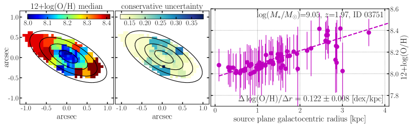
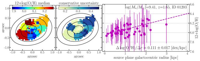
Figure 3.— Metallicity maps and radial gradient measurements of the two galaxies. The left panels show the 2D maps of the median value estimates of metallicity, and the central panels show their conservative uncertainties (i.e. the larger side of the asymmetric 1-$\sigma$ error bars). The right panels show the corresponding radial gradients measurements. The black contours again mark the source plane de-projected galacto-centric distances as in Figure 1. We adopted weighted Voronoi tessellation (Cappellari & Copin, 2003; Diehl & Statler, 2006), with a SNR of 10 on [O iii] for the binned metallicity maps. In the right column, these bins are plotted as individual data points. The dashed line denotes the linear regression from these points, with the measured radial slope shown at the bottom of each panel. For both galaxies, the radial gradient is strongly positive (i.e. inverted).

3.2. ${\rm SFR}$, stellar population age, and gas fraction

To understand the cause of the strongly inverted metallicity gradients seen in these dwarf galaxies, we combine their EL maps with HST broad-band photometry to derive 2D maps of $M_{\ast}$, ${\rm SFR}$, stellar population age, and gas surface density for each galaxy. The ${\rm SFR}$ is derived from extinction-corrected Balmer emission line flux. Maps of H$\beta$ and H$\gamma$ emission are shown in Figure 1. The H$\beta$/H$\gamma$ line ratio provides a measurement of nebular extinction although it is limited by the modest signal-to-noise of H$\gamma$. We obtain more precise results from HST photometry, by converting $B_{435}$-$I_{814}$ color maps to spatial distributions of stellar reddening $E_{\rm S}(B-V)$ (Daddi et al., 2004). Nebular reddening $E_{\rm N}(B-V)$ is then calculated following Valentino et al. (2017). The nebular reddening maps of both our galaxies show lower dust attenuation in centers than that in outskirts, consistent with the inverted metallicity gradients shown in Figure 3.

We calculate extinction in H$\beta$ adopting a Cardelli et al. (1989) dust extinction law (with $R_{\rm V}$ =3.1) and assuming Case B recombination with Balmer ratios appropriate for fiducial Hii region properties (i.e., H$\alpha$/H$\beta$ = 2.86). Finally, we convert intrinsic H$\alpha$ luminosity to ${\rm SFR}$ through the commonly used calibration (Kennicutt, 1998a),

$${\rm SFR}=4.6\times 10^{-42}\leavevmode\nobreak\ \frac{L(\textrm{H}\alpha)}{\rm erg/s}\quad[M_{\odot}/\textrm{yr}],$$ (2)

appropriate for the Chabrier (2003) IMF. This provides the instantaneous star formation rate on $\sim$10 Myr time scales; we note that the ultraviolet continuum probed by HST photometry is sensitive to recent ${\rm SFR}$ over a longer time span ($\sim$100-300 $\rm Myr$). The short timescales probed by Balmer emission are most relevant for determining outflow physical properties, which are highly dynamic on small spatial scales, e.g., at sub-kpc level.

Next we derive average stellar age maps, using the spatial distribution of EL EW as the primary constraint. We calculate H$\beta$ rest-frame EWs from our maps of the emission line flux and stellar continuum flux density. Stellar continuum maps are corrected for emission line contamination as described in Section 2. We correct for stellar Balmer absorption which we estimate to be rest-frame EW $\sim$3 Å in H$\beta$ based on the derived galaxy properties (Kashino et al., 2013). Maps of H$\beta$ EW are then converted to average stellar age using a series of Starburst99 stellar population synthesis models (Leitherer et al., 1999; Zanella et al., 2015) assuming 1/5 solar metallicity and constant star formation history.

We also compare the age estimates given by our SED fitting (Section 2) and H$\beta$ rest-frame EW using the method described above. The median values given by the former practice are systematically larger than those of the latter by $\sim$0.5 dex, but we note that the uncertainties by the SED fitting are usually much larger due to the absence of prominent continuum spectral age indicators, e.g., ${\rm D}_{n}(4000)$ and ${\rm H}\delta_{A}$ (Kauffmann et al., 2003). Hence, we adopt the results from H$\beta$ rest-frame EW as the average age for stellar populations throughout our paper, as we consider this a more reliable estimate.

Finally, we calculate the gas fraction defined as

$$f_{\rm gas}=\Sigma_{\rm gas}/\left(\Sigma_{\rm gas}+\Sigma_{\ast}\right).$$ (3)

Since we do not directly observe the bulk of interstellar gas, we instead estimate gas surface density $\Sigma_{\rm gas}$ by inverting the Kennicutt-Schmidt (KS) law (Schmidt, 1959; Kennicutt, 1998b), i.e., $\Sigma_{{\rm SFR}}\propto\Sigma_{\rm gas}^{N}$ together with our measurements of $\Sigma_{{\rm SFR}}$ described above. We adopt the more robust extended version of the KS law developed by Shi et al. (2011, 2018) which is especially useful in low density regimes:

$$\frac{\Sigma_{{\rm SFR}}}{M_{\odot}/\rm yr/\rm kpc^{2}}=10^{-4.76}\left(\frac{\Sigma_{\ast}}{M_{\odot}/\rm pc^{2}}\right)^{0.545}\left(\frac{\Sigma_{\rm gas}}{M_{\odot}/\rm pc^{2}}\right)^{1.09}.$$ (4)

This extended KS law has been tested in numerous ensembles of galaxies as well as low surface brightness regions in individual galaxies, and is shown to have relatively small scatter ($\sim$0.3 dex) over a large dynamic range of gas and ${\rm SFR}$ surface densities. We have combined in quadrature this systematic uncertainty of 0.3 dex in our estimates of $\Sigma_{\rm gas}$.

Figure 4 shows the derived 2D maps of ${\rm SFR}$, average stellar age, and gas fraction. In general, we observe centrally concentrated star formation, with the most actively star-forming regions having surface densities $\gtrsim 10\leavevmode\nobreak\ M_{\odot}/\rm yr/\rm kpc$. On average, the central regions also have older stellar populations and smaller gas fractions than the outskirts, indicating that the outer regions are still in the early stages of converting their gas into stars. These features together indicate that we are witnessing the rapid build-up of galactic disks through in-situ star formation and strongly support an inside-out mode of galaxy growth (Nelson et al., 2014; Jones et al., 2013).

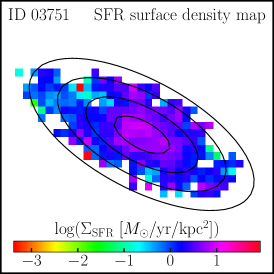
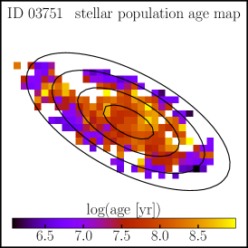
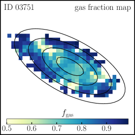
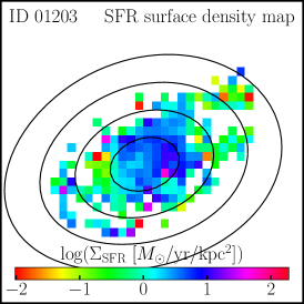
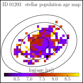
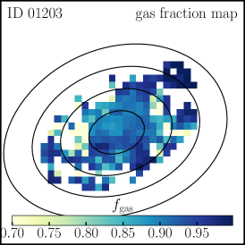
Figure 4.— Maps of SFR surface density, average stellar population age, and gas fraction for our galaxies, derived from our spatially resolved analysis of stellar continuum and nebular emission. The spatial extent and orientation follows that in Figure 1. We see that for both sources compared with their outskirts, their central regions have more active star formation, older stellar population, and lower gas fraction.

We compare our radially averaged $f_{\rm gas}$ and metallicity measurements against the predictions from the simple chemical evolution model developed by Erb (2008). To separate the effects of gas inflows and outflows, we compute two extreme sets of models, one being pure gas accretion (i.e. with no outflows, $f_{o}=\Psi/{\rm SFR}=0$) and the other corresponding to the leaky box model (i.e. with no inflows, $f_{i}=\Phi/{\rm SFR}=0$). The results are shown in Figure 5. We note that for the pure gas accretion scenario, $f_{\rm gas}$ cannot decrease beyond a certain value, i.e.,

$$f_{\rm gas}^{\rm min}=1-\frac{1-R}{f_{i}-f_{o}},$$ (5)

where $f_{o}=0$ and $R$ is the instantaneous return fraction. This $f_{\rm gas}^{\rm min}$, implicitly imposed by Eq. (11) of Erb (2008), physically indicates that galaxies cannot exhaust their gas reservoir to below a certain amount without the help of outflows, under the equilibrium condition with steady gas accretion (see Section 3.3 when this equilibrium assumption is relaxed). Therefore, the pure gas accretion scenario cannot explain the observed gas fractions in our source central regions (at $\lesssim$ 2$\rm kpc$) where metallicities are also lower. The leaky box model, on the other hand, provides a plausible explanation for our observation such that the outflow rate tends to increase towards galaxy center. However, we stress that in reality both gas outflows and inflows are acting together to re-distribute metallicity. This test using simple chemical evolution models just clearly shows that using gas accretions alone cannot explain our spatially resolved measurements.

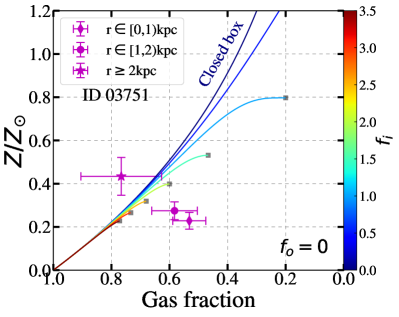
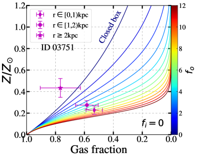
Figure 5.— Gas fraction and metallicity estimated in different radial annuli for galaxy ID03751. The diamond, circle, and star symbols represent measurements derived at a galacto-centric radius of $r\in[0,1)$$\rm kpc$, $r\in[1,2)$$\rm kpc$, and $r\gtrsim 2$$\rm kpc$, respectively. We also overlay the curves calculated from a simple chemical evolution model Erb (2008) under extreme conditions, i.e., pure gas inflow ($f_{o}=0$; left) and pure gas outflow ($f_{i}=0$; right). Note that the trajectories of pure gas inflow cases cease at the grey squares for high infall rate ($f_{i}\gtrsim 1$) conditions; any extensions from those grey squares toward low gas fraction (while fixing metallicity) are unphysical. This simple comparison shows that purely gas accretion does not suffice to explain the strong inverted gradients seen in our galaxies.

3.3. Spatially resolved gaseous outflows

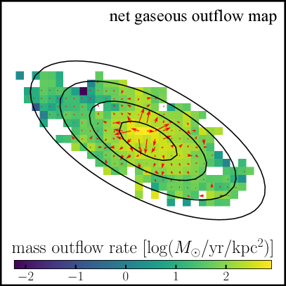
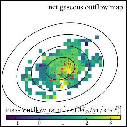
Figure 6.— Maps of gaseous outflow rates derived from our analysis combining gas regulator models and empirical star-formation laws. The spatial extent and orientation follows that in Figure 1. Red arrows show the net direction and magnitude of the gaseous outflows driven by galactic winds. We argue that outflows play a key role in effectively transporting stellar nucleosynthesis yields from the inner regions of these two galaxies to their outskirts.

The application of simple chemical evolution in Section 3.2 is enlightening but depends on strong assumption, such as that the azimuthal variations are negligible and galaxies live in equilibrium. In reality, these conditions might not be valid, e.g., due to rapid gas flows. To gain a more precise understanding of the physics of galactic winds and the role of gaseous outflows in shaping the observed spatial distribution of metallicity, independent of those assumptions, we can turn to a more advanced framework for galaxy chemical evolution: the gas regulator model (Lilly et al., 2013; Peng & Maiolino, 2014). This model provides an informative and coherent view of the full baryon cycle, involving the accretion of underlying DM halos, as well as the instantaneous regulation of star formation by a time-variable gas reservoir. A key feature of this model is that it does not assume that galaxies live in an equilibrium state, where the total amount of gas mass remains constant. The non-equilibrium flexibility is especially important for applying this model to spatially resolved regions within a galaxy, where gas may be transported radially from one region to another. Chemical evolution within the gas regulator model is described by the equations

$$Z_{\rm gas} =\left[Z_{0}+y\tau_{\rm eq}\epsilon\left(1-\exp(-\frac{t}{\tau_{\rm eq}})\right)\right]\left[1-\exp(\frac{-t/\tau_{\rm eq}}{1-\exp(-t/\tau_{\rm eq})})\right],$$ (6)

$$\tau_{\rm eq} =\frac{1}{\epsilon\left(1-R+\lambda\right)}.$$

Here we adopt the convention of symbols itemized in Table 1 of Peng & Maiolino (2014): $Z_{\rm gas}$ is the mass fraction of metals in the gas reservoir (determined from the observed $12+\log({\rm O/H})$ as in Peeples & Shankar (2011)), $t$ is the average stellar population age, $\tau_{\rm eq}$ is the time scale on which the baryon cycle reaches equilibrium, $\epsilon$ is the star-forming efficiency (defined as $\epsilon\equiv{\rm SFR}/M_{\rm gas}=\Sigma_{\rm SFR}/\Sigma_{\rm gas}$), and $\lambda$ is the mass loading factor (defined in terms of the mass outflow rate $\Psi$, such that $\lambda=\Psi/{\rm SFR}$). We adopt a stellar nucleosynthesis yield $y=0.003$ (Dalcanton, 2007) with $R=0.4$ estimated from BC03 (Bruzual & Charlot, 2003) stellar population models. Finally, we assume that gas inflows are pristine ($Z_{0}=0$).

For each spatial region where we have estimated the metallicity, ${\rm SFR}$, gas surface density, and age (Figures 3, 4), we solve the above equations for the mass loading factor $\lambda$ and subsequently calculate the mass outflow rate $\Psi$. The 2D distribution of $\Psi$ is displayed in Figure 6. Taking the gradient field of this gaseous outflow map, we obtain the net direction of the outflowing mass flux on sub-galactic scales, projected along the line of sight, denoted by the red arrows in Figure 6. The results demonstrate that strong galactic winds transport mass from the center to the outskirts, with the net radial transport of heavy elements causing the inverted gradients observed in our targets.

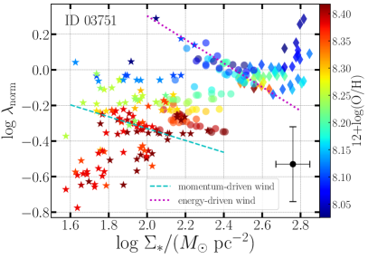
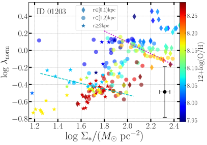
Figure 7.— Correlation between spatially resolved mass loading factor $\lambda$ (normalized to the value at radius 1 kpc; see Table 1) and stellar surface density $\Sigma_{\ast}$, color-coded by metallicity. As in Figure 4, the diamond, circle, and star symbols represent measurements derived at a galacto-centric radius of $r\in[0,1)$$\rm kpc$, $r\in[1,2)$$\rm kpc$, and $r\gtrsim 2$$\rm kpc$, respectively. We overlay as an illustration two scaling relations that are commonly assumed to describe integrated measurements: $\lambda\propto\Sigma_{\ast}^{-2/3}$ for an energy-driven wind model marked by magenta dotted lines, and $\lambda\propto\Sigma_{\ast}^{-1/3}$ for a momentum-driven wind model by cyan dashed lines. Evidently, a single scaling relation is not sufficient to describe the spatially resolved data, demonstrating the need for a more sophisticated approach. The black point in the lower right corner in each panel displays the median uncertainties for these measurements.

The distribution of mass loading factors $\lambda$ within each of our targets is also shown in Figure 7, revealing higher $\lambda$ (and therefore a higher fraction of metals lost) in the central regions. This preferential removal of metals from the center, and subsequent deposition at larger radii, gives rise to the strong positively sloped metallicity gradients evident in Figure 3. The high values of $\lambda$ have important implications for the role of feedback in galaxy formation. Most fundamentally, our results support feedback as a solution to the “over-cooling” problem in galaxy formation, by ejecting gas and preventing overly condensed baryonic regions at high redshifts (White & Rees, 1978; Dekel & Silk, 1986). Such strong outflows are also expected to suppress the formation of stellar bulges from low angular momentum gas (Governato et al., 2010; Brook et al., 2012). This is consistent with low bulge fraction in these two galaxies measured from high resolution HST imaging (Table 1).

A key feature in the $\lambda$ distribution is that neither of the wind modes, driven by momentum or energy conservation, can explain the behavior of the mass dependence of $\lambda$ alone, within individual galaxies. Outflows are typically parameterized by either a momentum-driven (Oppenheimer & Davé, 2006, 2008) or an energy-driven (Springel & Hernquist, 2003) wind mode, both of which are physically well motivated (Murray et al., 2005). The energy-driven wind scenario assumes that outflows are launched by the thermal pressure of supernova (SN) explosions and/or winds from massive stars. A portion of this thermal energy provides the outflow kinetic energy, i.e., $\Psi\times v^{2}_{\rm wind}\sim{\rm SFR}$, where the wind speed $v_{\rm wind}$ can mimic the escape velocity from DM halo, i.e., $v_{\rm esc}\sim M_{\rm h}^{1/3}$ given by the virial theorem. This results in the scaling relation of $\lambda\propto M_{\ast}^{-2/3}$, assuming the linear correlation between the mass constituents of stellar and dark components. The energy-driven wind model is found successful in explaining the low abundance of satellite galaxies in the Milky Way (Okamoto et al., 2010). The momentum-driven wind model instead relies on the momentum injection deposited by radiation pressure from SN explosions and/or massive stars, leading to $\Psi\times v_{\rm wind}\sim{\rm SFR}$ and $\lambda\propto M_{\ast}^{-1/3}$. In this scenario, $v_{\rm wind}$ is proportional to $M_{\ast}$ and ${\rm SFR}$, broadly consistent with some observational results (Martin, 2005). The transition from energy- to momentum-driven winds is typically thought to be a galaxy-wide phenomenon, resulting in the steepening of the mass-metallicity relation below $M_{\ast}$ $\simeq 10^{9.3}$$M_{\odot}$ at $z\simeq 2$ (Henry et al., 2013b). However, our analysis indicates that a single mode is not sufficient to describe spatially resolved data within one galaxy and it is highly likely that the transition from energy- to momentum-driven winds occurs on sub-galactic scales, governed by local gas and star formation properties in addition to the global gravitational potential.

4. Summary and discussion

We present the first robust confirmation of the existence of strongly inverted metallicity radial gradient (i.e. $\gtrsim$0.1 dex/kpc) in star-forming dwarf galaxies ($M_{\ast}\lesssim 10^{9}M_{\odot}$) at the peak of star formation and chemical enrichment ($z\sim 2$). Our synergy of the diffraction-limited imaging spectroscopy from HST NIR grisms and lensing magnification permits exquisite spatial sampling, i.e., at the scale of 50-100 pc, to securely resolve our $z\sim 2$ galaxies with $\gtrsim$300 resolution elements (Figures 1–3) to deliver precise radial gradient measurements. To understand the physical origin of these strongly inverted gradients, we obtain high resolution 2D maps of star formation rate, characteristic stellar age (or equivalently star formation timescale), and gas fraction, from HST observations of source stellar continuum and nebular emission. These 2D maps show that the galactic disks of our sources are rapidly assembling stellar mass through in-situ star formation, in the early phase of inside-out growth (Figure 4). By comparing our observations with simple chemical evolution models, we find that gas accretion alone cannot explain these strongly inverted gradients in our galaxies (Figures 5).

Using a more advanced gas regulator model, we are able to calculate the spatial distribution of mass loss rates from outflows, treating each spaxel as an independent star-forming region, and thus map the macroscopic patterns of net gaseous outflows (Figure 6). It turns out that the mass loss rates are highest in the central regions of both galaxies, coincident with the peak star formation surface densities. A natural explanation is thus that active star formation in galaxy centers gives rise to powerful winds that transport gas and metals away from the center toward larger radii, forming “galactic fountains” (Martin et al., 2002).

Furthermore, our spatially resolved analysis of metals, ${\rm SFR}$, and stellar populations shows that a single type of wind mechanism (either energy or momentum driven) cannot explain the entire galaxy (Figure 7). A primary physical parameter that has been proposed to set the transition between the two wind dynamics is the gravitational potential, often parameterized by velocity dispersion ($\sigma$). There exists a critical scale $\sigma_{\rm crit}$ (Murray et al., 2005) such that for galaxies with $\sigma<\sigma_{\rm crit}$, energy injection by SNe sets a limiting ${\rm SFR}$ above which interstellar gas is ejected in galactic winds. For galaxies with $\sigma>\sigma_{\rm crit}$, momentum deposition limits the maximum ${\rm SFR}$ above which the ISM is likewise ejected. The presence of both energy- and momentum-driven wind scalings in one galaxy suggests that feedback-triggered winds are connected to physical properties on sub-galactic scales, e.g., local velocity dispersion ($\sigma_{\rm local}$), which is sensitive to the optical depth of gas flows, the coupling efficiency between gas clouds and dust parcels, etc.. On sub-galactic scales, there exists a strong correlation among velocity dispersion (not necessarily $\sigma_{\rm local}$), surface density and size of molecular clouds (see Ballesteros-Paredes et al., 2011, and references therein). It appears that in our galaxies, the wind-launching mechanism transitions from energy- to momentum-driven as galacto-centric radius increases. This gives rise to a hypothesis that $\sigma_{\rm local}$ in our galaxies should increase from inner to outer regions. Our current kinematic data on source ID01203 have high spatial resolution (at $0\farcs 05$ plate scale) yet narrow FoV so that it is infeasible to map sub-kpc scale velocity dispersion accurately to outer regions at $r\gtrsim 2$ $\rm kpc$, where momentum-driven wind seems to take over. To test this hypothesis conclusively, more spatially resolved data taken under sufficient spatial sampling will be required to robustly derive a full 2D map of velocity dispersion out to the periphery of the galactic disk, using instruments with relatively large FoV, e.g., the JWST NIRSpec IFU (Kalirai, 2018).

Physically, the momentum-driven wind scaling applies to “cool” ($T\sim 10^{4}$ K) ambient interstellar gas entrained in outflows, whereas the energy-driven wind is appropriate when entrained gas is shock heated to temperatures where cooling is inefficient ($T\sim 10^{6}$ K). A plausible scenario for our galaxies is that feedback from an intense burst of star formation in the central regions heats the ejected gas to a highly ionized phase, while gas entrained in outflows from the outer regions remains cool. If this interpretation is correct, then we expect a distinct signature in the absorption properties of outflowing gas. Outflows from the central regions should be dominated by highly ionized species (e.g. O vi, C iv, Si iv) whereas outflows from the outer regions should have relatively more of the low ions characteristic of $T\sim 10^{4}$ K gas (e.g. Fe ii, Mg ii, Si ii). Both high and low ion species are commonly observed in outflows from star forming galaxies at $z\simeq 2$ (Berg et al., 2018; Du et al., 2018), although their spatial distributions are not yet well known (but see James et al., 2018). Our hypothesis suggests a more central concentration of the high ions in the specific cases where a combination of both outflow scalings results in inverted metallicity gradients. This prediction can be directly tested with spatially resolved spectroscopy of rest-frame ultraviolet absorption lines using instruments such as Keck/KCWI or VLT/MUSE.

Appendix A Extracting and fitting 1D and 2D HST grism spectra

As briefly mentioned in Section 2.2, we employed the Grism Redshift and Line analysis software Grzili to reduce the HST WFC3/NIR grism data from raw exposures acquired by the GLASS program. Our primary goal is to obtain the spatially resolved emission line intensities after removing the contribution from source continuum. In terms of modeling the continuum spectrum, Grzili first produces a simple flat (in $F_{\lambda}$) spectral model for all sources within the WFC3 FoV with $H_{160}$-band magnitude brighter than 26 ABmag. The normalization is determined to match the flux in the corresponding reference image (in our cases, F105W as the reference to G102, and F140W to G141, ascribed to similar wavelength coverage). Then second-order polynomial functions are fitted to the sources whose $H_{160}$-band magnitude is brighter than 24 ABmag. This process is done iteratively, until a convergence point where the residual in the grism exposures after subtracting the fitted continuum models becomes negligible.

While the polynomially fitted continuua serve as good enough models for contamination subtraction associated with neighboring objects, this polynomial functional form is clearly not physically representative of the actual SED of the underlying stellar continuum for our sources of interest. To facilitate a more accurate continuum subtraction, we further refine the source continuum model by considering primarily four template continuum spectra in a range of characteristic ages for stellar populations:

1. a low-metallicity Lyman-break galaxy (Q2343-BX418) showing very young, blue continuum (Erb et al., 2010),

2. an intermediate-age composite SED with moderate Balmer break and 4000 Å break, synthesized in Brammer et al. (2008) following the method of Blanton & Roweis (2007),

3. a post-starburst SED showing prominent Balmer break and 4000 Å break from the UltraVISTA survey (Muzzin et al., 2013),

4. a single stellar population SED with a 13.5 Gyr age and solar metallicity (Conroy & van Dokkum, 2012).

This combination of both empirical and synthetic SED templates constitutes an optimized set appropriate for redshift fitting and continuum subtraction under our situation. As discussed in Brammer et al. (2008), there is a trade-off between the number of templates used in SED fitting and numerical efficiency, and they find that the improvement is negligible if the number of templates is increased to above 5. For a sanity check, we also run the template fitting procedures using a more complete template library built from the Flexible Stellar Population Synthesis (FSPS) models (Conroy et al., 2009, 2010; Conroy & Gunn, 2010) and found no noticeable changes in the spectroscopic redshift determinations nor continuum subtractions.

In addition to fitting stellar continuum, we model the intrinsic nebular emission lines in 1D spectra as Gaussian functions. The amplitudes and flux ratios between most of the line species are allowed to vary (except for some certain line complexes, e.g., $f_{[\textrm{O}\leavevmode\nobreak\ \textsc{iii}]\leavevmode\nobreak\ 5008}/f_{[\textrm{O}\leavevmode\nobreak\ \textsc{iii}]\leavevmode\nobreak\ 4960}$ = 3:1). Given the relatively low instrument resolution of HST grisms, the dynamic motion of gas and stellar components leave no effect on the observed profiles (both in 1D and 2D) of line emission/absorption features. However, for spatially extended sources, the effective spectral resolution is lowered by morphological broadening (van Dokkum et al., 2011), which usually varies with respective to the light-dispersion direction, i.e., the position angle (P.A.). We explicitly take the source morphology into account via convolving the model spectra (stellar continuum + nebular emission) with the direct image in reference frames averaged along light-dispersion directions.

As a result, in Figures 8 and 9, we show the observed and fitted grism spectra for both of our sources at separate P.A.s. Albeit slightly different in shape and slope, the red curves in 1D spectra comes from the same best-fit spectral model for each source and the difference is due to slightly varying morphological broadening. We also see that the 2D continuum-subtracted spectra are sufficiently clean, preserving only the nebular emission features that we later combined to get the spatially resolved emission line maps shown in Figure 1.

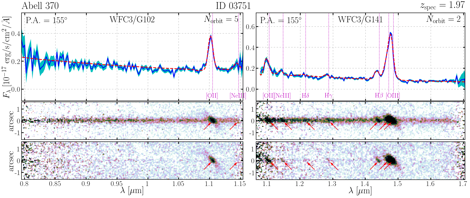
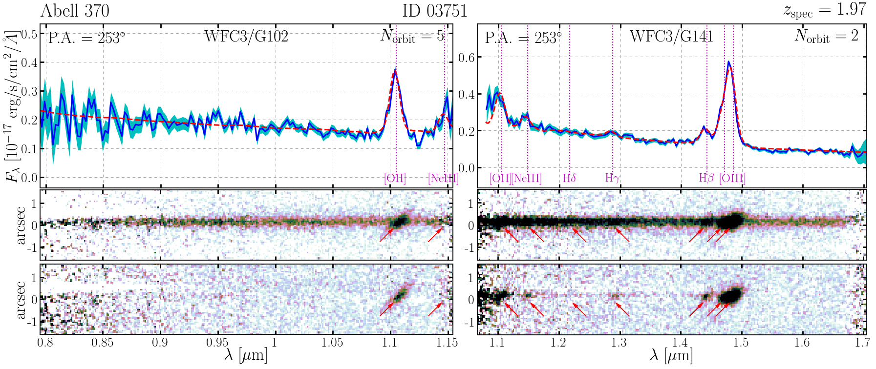
Figure 8.— The HST grism spectra for source ID03751 in the field of Abell 370 taken by the GLASS program. The total science integration is equally distributed into two separate P.A.s, reaching 5 orbits of G102 exposures and 2 orbits of G141 exposures per P.A., shown in two sub-figures. In each sub-figure, from top to bottom, we show the optimally extracted 1D spectra and the full 2D spectra before and after source continuum subtraction, for both grism elements. On the 1D spectra, the observed flux is represented by the blue solid line with 1-$\sigma$ noise level denoted by the cyan shaded band, and the 1D model spectrum (source continuum + nebular emission) is represented by the red dashed curve. The observed locations of emission features are highlighted by vertical dotted lines in magenta and arrows in red, in 1D and 2D spectra respectively. Note that due to low spectral resolution, [Ne iii] is blended with He i$\lambda 3889$+H8 on the red side and H9 on the blue side.

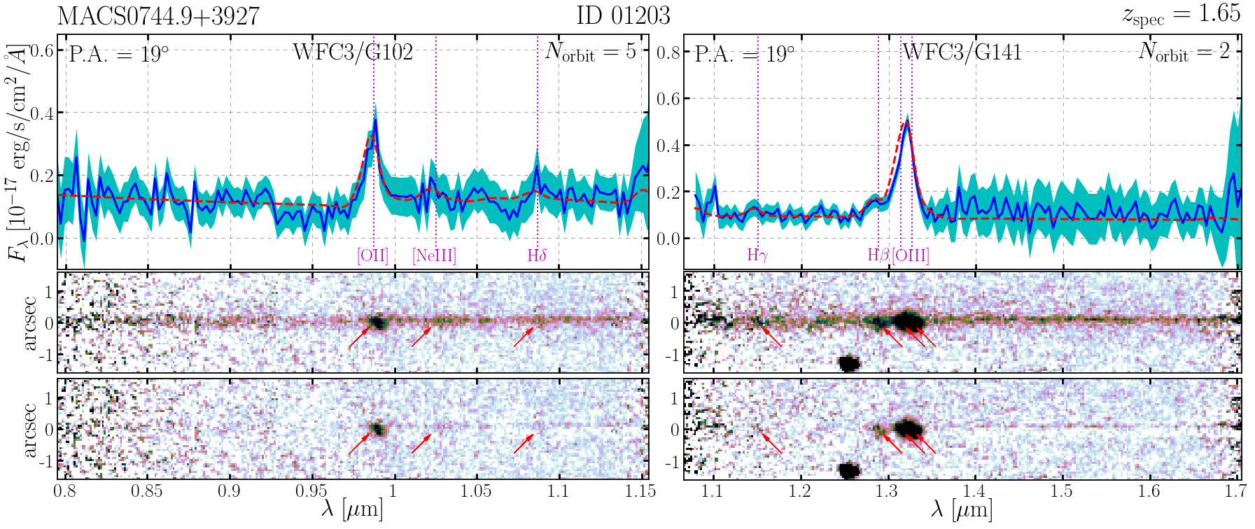
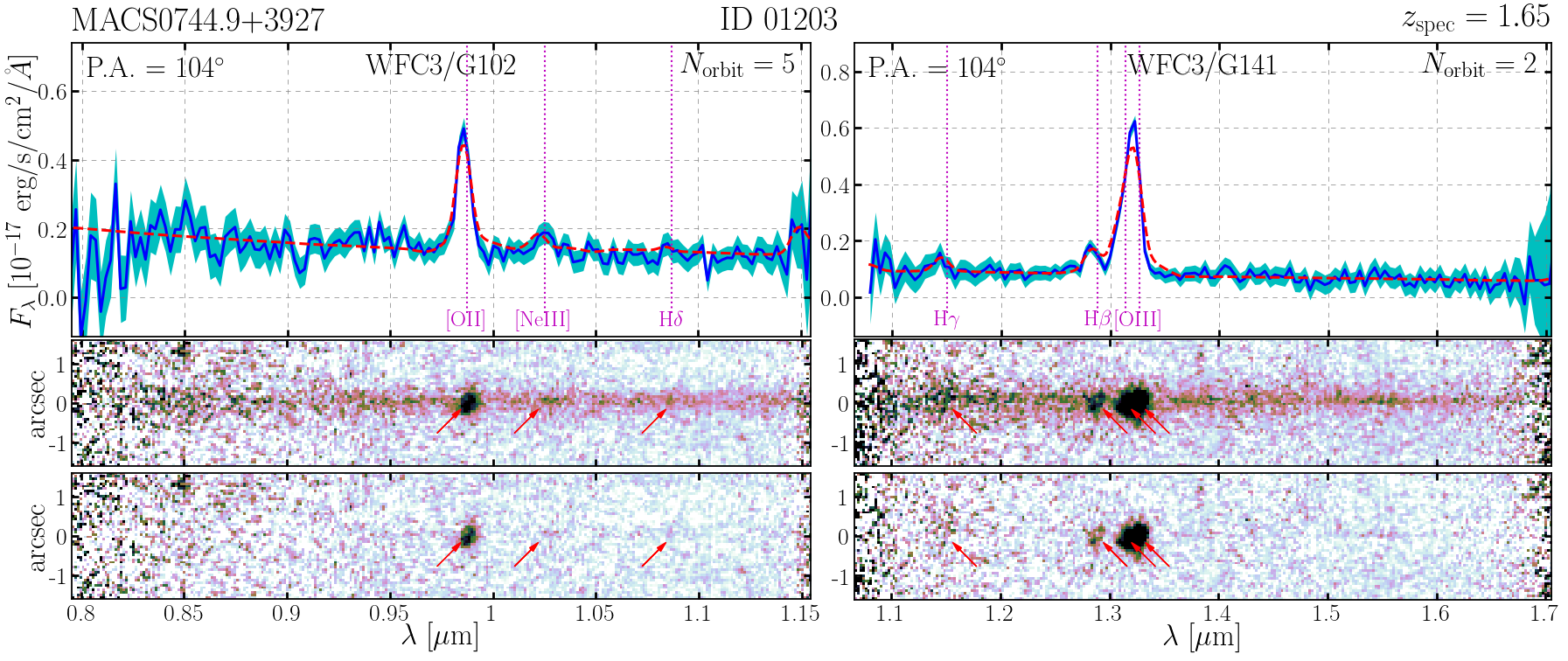
Figure 9.— Same as Figure 8, except that source ID01203 in the field of MACS0744.9+3927 is shown.

Appendix B Gas kinematics from Keck OSIRIS observations

Kinematics of Hii regions are of interest both for determining whether rotating gaseous disks are present, and the overall scale of velocity dispersion which is thought to correlate with the mode of feedback. We have obtained kinematic maps from H$\alpha$ emission for source ID01203 as part of a GLASS followup campaign with the OSIRIS integral field spectrograph (Larkin et al., 2006) on the Keck I telescope. Full details of the observations and analysis are presented elsewhere (Hirtenstein et al., 2018); here we give a brief summary. Data were obtained on 2016 October 21 using the Hn5 filter, 50 milliarcsecond scale, and laser guide star AO, which provides the excellent spatial sampling needed to resolve velocity structure on the relevant $\sim$0$\farcs$1 scales. We obtained 3 exposures of 900 seconds each. The OSIRIS Data Reduction Pipeline was used to process the data, following the standard methods adopted in our previous work (Jones et al., 2013). We fit H$\alpha$ line emission in each spaxel with a Gaussian function, requiring $\geq 5\sigma$ significance for acceptable fits. Gas rotation velocity ($V$) and velocity dispersion ($\sigma$) are determined from the Gaussian centroid and width. We correct velocity dispersions for the effects of instrument resolution and beam smearing by subtracting these terms in quadrature from the best-fit Gaussian dispersion. The median beam smearing correction is a 7% reduction in $\sigma$.

Resulting maps of $V$ and $\sigma$ in Figure 10 reveal a sheared velocity field with high local velocity dispersion ($\gtrsim 50$ $\rm km\leavevmode\nobreak\ s^{-1}$), common among disk galaxies at similar redshift. To quantify the degree of rotational support, we extract a 1D velocity profile along the kinematic major axis. We fit this with the circular rotation curve of an exponential disk mass profile. The disk rotation curve is in good agreement with the data, with maximum velocity $V\sin i=94\pm 7$ $\rm km\leavevmode\nobreak\ s^{-1}$. Here $i$ is the disk inclination angle relative to the line-of-sight. The pixel-averaged $\sigma=73\pm 3$ $\rm km\leavevmode\nobreak\ s^{-1}$ such that we derive $V/\sigma=(1.3\pm 0.1)/\sin i$ indicating orderly rotation in spite of a high level of ISM turbulence. This $V/\sigma$ ratio is typical of the galaxy population harboring thick disks at similar mass and redshift (Wisnioski et al., 2015; Leethochawalit et al., 2016).

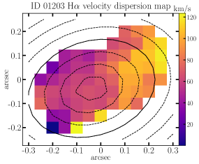
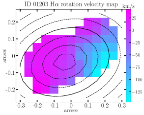
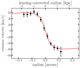
Figure 10.— H$\alpha$ emission kinematics of ID01203 from our OSIRIS AO-assisted observations showing the velocity dispersion (left), the rotation velocity (center), and rotation curve extracted along the major axis (right). The overlaid contours in the left and center panels also represent the source plane de-projected galacto-centric radii, but in 0.25 kpc interval. To give relative scale with respect to our HST stamps, the 1 kpc radius contour is still in solid. The red curve in the right panel is the best-fit rotation curve for an exponential disk mass distribution, giving a maximum line-of-sight velocity $V\sin i=94\pm 7$ $\rm km\leavevmode\nobreak\ s^{-1}$. The data are in good agreement with a thick disk rotation curve despite a high level of turbulence.

Appendix C A comparative study of metallicity gradients derived using different strong line calibrations

Generally speaking, three approaches exist in deriving metallicity information in extragalactic sources from spectroscopic observations: the metal recombination line method, the electron temperature $T_{\rm e}$ (“direct”) method, and the strong emission line calibration method (see e.g., Blanc et al., 2015; Bianco et al., 2015; Maiolino & Mannucci, 2018, for recent reviews).

The first method is believed to be the most direct measurement of the chemical abundances, as the emissivities of the permitted recombination lines of metal ions are only weakly dependent on $T_{\rm e}$ and the electron density $n_{\rm e}$ of the ionized media. Yet these recombination lines are extremely weak, usually $\sim 10^{-3}-10^{-4}$ fainter than the hydrogen recombination lines, even for the most abundant metal elements like carbon and oxygen. So the first method is only feasible not far beyond the local group (see recent results by e.g., García-Rojas & Esteban, 2007; López-Sánchez et al., 2007; Bresolin et al., 2009; Esteban et al., 2009).

The second method resorts to the CELs of metal ions, given that their emissivities depend strongly on $T_{\rm e}$ of the ionized gas, hence this method is usually coined the $T_{\rm e}$ method. The flux ratios of the temperature-sensitive auroral to nebular CELs (e.g. $[\textrm{O}\leavevmode\nobreak\ \textsc{iii}]\lambda 4363$/$[\textrm{O}\leavevmode\nobreak\ \textsc{iii}]\lambda 5008$) are often adopted to estimate $T_{\rm e}$. Yet the auroral lines are intrinsically too faint — usually at the percent level of the strong nebular lines — to be observable in individual galaxies at high redshifts and high metallicity (corresponding to low $T_{\rm e}$). There are only a handful of such detections to date (Christensen et al., 2012; Stark et al., 2013; James et al., 2014; Sanders et al., 2016; Gburek et al., 2019).

To solve the limitations of the $T_{\rm e}$ method, and entail efficient determinations of chemical abundances in faint Hii regions in the high-$z$ universe, numerous authors rely on the calibrations of flux ratios involving bright nebular CELs ([O iii], [O ii], [N ii], etc.) and Balmer lines (H$\alpha$, H$\beta$) as a proxy for metallicity (i.e. the strong line calibration method). These strong lines are among the most accessible species of nebular line emission at high redshifts, thus rendering this third method the most viable approach to estimate metallicity at extragalactic distances. The line flux ratios can be calibrated against direct $T_{\rm e}$ measurements in galactic Hii regions and nearby individual or stacked galaxy spectra (Pilyugin, 2000, 2001; Pettini & Pagel, 2004; Pilyugin & Thuan, 2005; Pilyugin et al., 2010, 2012; Jones et al., 2015a; Brown et al., 2016; Gebhardt et al., 2015; Pilyugin & Grebel, 2016; Curti et al., 2017; Bian et al., 2018). These calibrations are often referred to as empirical calibrations. Another kind of calibrations is based on the theoretical predictions given by photoionization models (Edmunds & Pagel, 1984; McCall et al., 1985; McGaugh, 1991; Zaritsky et al., 1994; Kewley & Dopita, 2002; Kobulnicky & Kewley, 2004; Nagao et al., 2011; Dopita et al., 2013; Strom et al., 2017), and therefore known as theoretical calibrations. In addition, several authors devise a “hybrid” calibration via combining both kinds of line ratio results (Denicoló et al., 2002; Nagao et al., 2006; Maiolino et al., 2008).

Albeit the strong line calibration method is most widely used, we must warn the readers of some potential systematics associated with it. For instance, Kewley & Ellison (2008) show that different calibrations produce offsets in the absolute scale of the mass-metallicity relation as large as 0.7 dex (also see e.g., Moustakas et al., 2010; López-Sánchez et al., 2012, for similar conclusions). This primarily originates from the different treatments and assumptions of some secondary parameters that also affect the brightness of strong nebular CELs, e.g., the ionization parameter, hardness of ionizing spectrum, the nitrogen vs. oxygen abundance ratio, the cosmic evolutions of $T_{\rm e}$ and $n_{\rm e}$, etc..

In particular, the flux ratio of $[\textrm{N}\leavevmode\nobreak\ \textsc{ii}]\lambda 6583$ and H$\alpha$ is one of the most frequently calibrated metallicity diagnostics. But it essentially traces the relative abundance of nitrogen, instead of oxygen, with respect to hydrogen. There have been reported large offset (0.2-0.4 dex) between the loci of star-forming galaxies locally from SDSS and at high-$z$ in the BPT diagram (Steidel et al., 2014; Shapley et al., 2015; Strom et al., 2016). This indicates that extending the locally calibrated strong line diagnostics involving nitrogen to high-$z$ can be potentially problematic, due to the evolving ionization conditions in the ISM (Strom et al., 2017).

On the other hand, the flux ratios between oxygen CELs and H$\beta$ are also popular diagnostics, particularly R₂₃=$(f_{[\textrm{O}\leavevmode\nobreak\ \textsc{iii}]\lambda 5008}+f_{[\textrm{O}\leavevmode\nobreak\ \textsc{iii}]\lambda 4960}+f_{[\textrm{O}\leavevmode\nobreak\ \textsc{ii}]})/f_{\textrm{H}\beta}$. However, due to its bi-modality, one often has to pre-determine the locations of metallicity branches before applying it (López-Sánchez & Esteban, 2010; Guo et al., 2016). This has presented some challenges especially when the source of interest is believed to be located in the transition regions between the two branches. This dilemma can be effectively alleviated when the ionization and excitation states of the ionized gas are taken into account (Kobulnicky & Kewley, 2004; Pilyugin & Thuan, 2005; Jiang et al., 2019).

Table 2Coefficients for the strong line metallicity calibrations used and tested in this work.

Group	$\log R$	$c_{0}$	$c_{1}$	$c_{2}$	$c_{3}$	$c_{4}$	$\sigma_{\log R}$ [dex]
Maiolino et al. (2008) calibrations
O3Hb-O2Hb	[O iii]/H$\beta$	0.1549	-1.5031	-0.9790	-0.0297	$\cdots$	0.1
	[O ii]/H$\beta$	0.5603	0.0450	-1.8017	-1.8434	-0.6549	0.15
R23-O3O2	R23	0.7462	-0.7149	-0.9401	-0.6154	-0.2524	0.05
	[O iii]/[O ii]	-0.2839	-1.3881	-0.3172	$\cdots$	$\cdots$	0.22
Jones et al. (2015a) calibrations
O3Hb-O2Hb	[O iii]/H$\beta$	-88.4378	22.7529	-1.4501	$\cdots$	$\cdots$	0.1
	[O ii]/H$\beta$	-154.9571	36.9128	-2.1921	$\cdots$	$\cdots$	0.15
R23-O3O2	R23	-54.1003	13.9083	-0.8782	$\cdots$	$\cdots$	0.06
	[O iii]/[O ii]	17.9828	-2.1552	$\cdots$	$\cdots$	$\cdots$	0.23
Curti et al. (2017) calibrations
O3Hb-O2Hb	[O iii]/H$\beta$	-0.277	-3.549	-3.593	-0.981	$\cdots$	0.09
	[O ii]/H$\beta$	0.418	-0.961	-3.505	-1.949	$\cdots$	0.11
R23-O3O2	R23	0.527	-1.569	-1.652	-0.421	$\cdots$	0.06
	[O iii]/[O ii]	-0.691	-2.944	-1.308	$\cdots$	$\cdots$	0.15

Note. — The value of the corresponding EL flux ratio is calculated by the polynomial functional form, i.e., $\log{R}=\sum_{i}c_{i}\cdot x^{i}$, where $x=12+\log({\rm O/H})-8.69$ for the Maiolino et al. (2008) and Curti et al. (2017) calibrations, and $x=12+\log({\rm O/H})$ for the Jones et al. (2015a) calibrations.

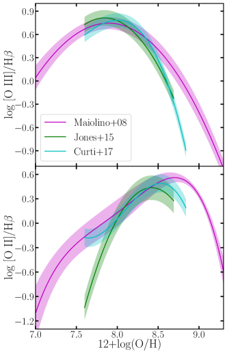
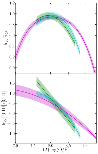
Figure 11.— The strong line metallicity calibrations used and tested in this work. The group of “O3Hb-O2Hb” calibrations is shown on the left, whereas the “R23-O3O2” group on the right. The corresponding coefficients of these calibrations from all three compilations are presented in Table 2.

While a detailed quantitative comparison of metallicity gradient measurements from different strong line calibrations is well beyond the scope of this work, we want to verify that our results are not significantly altered by the choice of metallicity diagnostics. For this purpose, we employ two of the most up-to-date pure empirical (i.e. calibrated against the actual $T_{\rm e}$ metallicities only) strong line calibrations. Curti et al. (2017) stacked a large number of SDSS galaxy spectra in the redshift range of $0.027<z<0.25$ to entail high SNR detection of the auroral [O iii] $\lambda$4363 lines in the high-metallicity branch, and therefore homogeneously calibrate the strong line flux ratios over wide metallicity range. Jones et al. (2015a) first extended the strong line calibrations to $z\sim 0.8$ using a sample of galaxies with [O iii] $\lambda$4363 detected in the DEEP2 Galaxy Redshift Survey. Apart from testing the metallicity diagnostics of $f_{[\textrm{O}\leavevmode\nobreak\ \textsc{iii}]}/f_{\textrm{H}\beta}$ and $f_{[\textrm{O}\leavevmode\nobreak\ \textsc{ii}]}/f_{\textrm{H}\beta}$ (i.e. group “O3Hb-O2Hb”) from these independently derived calibration sets, we also employed an alternative group of calibrations (combining R₂₃ and $f_{[\textrm{O}\leavevmode\nobreak\ \textsc{iii}]}/f_{[\textrm{O}\leavevmode\nobreak\ \textsc{ii}]}$, i.e., group “R23-O3O2”) in replacement of the “O3Hb-O2Hb” ratio diagnostics from the same calibration frameworks. The coefficients of these calibrations are given in Table 2, with their behaviors shown in Figure 11. We note that the results of Jones et al. (2015a) demonstrate that oxygen strong line diagnostics based on the $T_{\rm e}$ method remain reliable at moderate to high redshifts, thus supporting the conclusions of this paper.

Following similar procedures detailed in Section 3, we measure the radial metallicity gradients of our sources using these different groups of strong line diagnostics from independent calibration sets. The measurement results are summarized in Table 3. We find that although some systematic differences — as large as 0.06 dex/kpc — can be seen in the absolute values of the gradient slope, a positive radial gradient is always derived at high statistical significance for both of our galaxies, i.e., $\gtrsim 12\sigma$ for ID03751 and $\gtrsim 5\sigma$ for ID01203, regardless of which group of diagnostics from which calibration works is adopted. Figures 12 and 13 display the metallicity maps and radial gradients determined using the “O3Hb-O2Hb” group of Jones et al. (2015a) and Curti et al. (2017) calibrations for galaxies ID03751 and ID01203, respectively.

Table 3Inverted radial metallicity gradients measured from two different groups of metallicity diagnostics of three independent strong line calibration frameworks.

Galaxy	Calibration reference	Group	$\Delta\log({\rm O/H})/\Delta r$	Significance of detection
			[dex/kpc]	[# of $\sigma$]
ID 03751	Maiolino et al. (2008)	O3Hb-O2Hb	0.122$\pm$0.008	15.2
		R23-O3O2	0.087$\pm$0.007	12.4
	Jones et al. (2015a)	O3Hb-O2Hb	0.070$\pm$0.005	14.0
		R23-O3O2	0.060$\pm$0.005	12.0
	Curti et al. (2017)	O3Hb-O2Hb	0.085$\pm$0.006	14.2
		R23-O3O2	0.083$\pm$0.006	13.8
ID 01203	Maiolino et al. (2008)	O3Hb-O2Hb	0.111$\pm$0.017	6.5
		R23-O3O2	0.085$\pm$0.011	7.7
	Jones et al. (2015a)	O3Hb-O2Hb	0.086$\pm$0.013	6.6
		R23-O3O2	0.094$\pm$0.010	9.4
	Curti et al. (2017)	O3Hb-O2Hb	0.090$\pm$0.016	5.6
		R23-O3O2	0.100$\pm$0.010	10.0

We also perform a simple test using the theoretical calibrations by Strom et al. (2017), based on the latest results of the photoionization models incorporating the hard ionizing radiation from massive star binary systems as clearly revealed in the KBSS-MOSFIRE dataset (Steidel et al., 2014; Strom et al., 2016). Since Strom et al. (2017) did not prescribe the “O3Hb-O2Hb” calibrations as a function of $12+\log({\rm O/H})$ explicitly, we infer the metallicities in the radial bins of our sources using the metallicity indicator “$X_{\rm O32-R23}$” (see their Eq. 8). Using the dust-corrected line flux ratios shown in Figure 2, we obtain the metallicity estimates of 8.39(8.34) and 8.43(8.46) in the most inner and outer radial annuli of source ID03751(ID01203), respectively, again confirming the inverted nature of their radial gradient slopes.

For the sake of consistency with our previous and ongoing metallicity gradient analyses (Jones et al., 2015b; Wang et al., 2017, and Wang et al. in prep), we decide to keep the gradient measurements derived with the Maiolino et al. (2008) O3Hb-O2Hb calibrations as our default results.

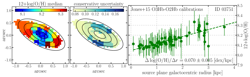
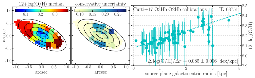
Figure 12.— Metallicity maps and radial gradients of source ID03751, determined assuming the Jones et al. (2015a) (top) and Curti et al. (2017) (bottom) “O3Hb-O2Hb” group of calibrations. As in Figure 3, in each row, the left panel shows the median value estimates of metallicity in individual Voronoi bins and the central panel shows the corresponding conservative uncertainties. In the right panel, these metallicity estimates are plotted against their source-plane de-projected galactocentric radii. The dashed line represents the best-fit linear regression with the radial gradient slope denoted on the bottom. Albeit different in the exact values of the slope, the gradients are always determined to be strongly inverted, with 0.070$\pm$0.005 (14.0$\sigma$) assuming the Jones et al. (2015a) “O3Hb-O2Hb” calibrations and 0.085$\pm$0.006 (14.2$\sigma$) for the Curti et al. (2017) “O3Hb-O2Hb” calibrations.

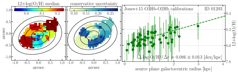
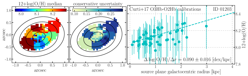
Figure 13.— Same as Figure 12, except that source ID01203 is shown. Again we see that strongly inverted gradients emerge from our measurements, i.e., 0.086$\pm$0.013 (6.6$\sigma$) and 0.090$\pm$0.016 (5.6$\sigma$) for the Jones et al. (2015a) and Curti et al. (2017) “O3Hb-O2Hb” calibrations, respectively.

References

- Abazajian et al. (2009) Abazajian, K. N., Adelman-McCarthy, J. K., Agüeros, M. A., et al. 2009, The Astrophysical Journal Supplement Series, 182, 543
- Andrews & Martini (2013) Andrews, B. H., & Martini, P. 2013, The Astrophysical Journal, 765, 140
- Ballesteros-Paredes et al. (2011) Ballesteros-Paredes, J., Hartmann, L. W., Vázquez-Semadeni, E., Heitsch, F., & Zamora-Avilés, M. A. 2011, Monthly Notices of the Royal Astronomical Society, 411, 65
- Belfiore et al. (2017) Belfiore, F., Maiolino, R., Tremonti, C. A., et al. 2017, Monthly Notices of the Royal Astronomical Society, 469, 151
- Berg et al. (2018) Berg, D. A., Erb, D. K., Auger, M. W., Pettini, M., & Brammer, G. B. 2018, The Astrophysical Journal, 859, 164
- Berg et al. (2015) Berg, D. A., Skillman, E. D., Croxall, K. V., et al. 2015, The Astrophysical Journal, 806, 16
- Bertin & Arnouts (1996) Bertin, E., & Arnouts, S. 1996, Astronomy and Astrophysics Supplement Series, 117, 393
- Bian et al. (2018) Bian, F., Kewley, L. J., & Dopita, M. A. 2018, The Astrophysical Journal, 859, 175
- Bianco et al. (2015) Bianco, F. B., Modjaz, M., Oh, S. M., et al. 2015, eprint arXiv:1505.06213, 54
- Birnboim & Dekel (2003) Birnboim, Y., & Dekel, A. 2003, Monthly Notices of the Royal Astronomical Society, 345, 349
- Blanc et al. (2015) Blanc, G. A., Kewley, L. J., Vogt, F. P. A., & Dopita, M. A. 2015, The Astrophysical Journal, 798, 99
- Blanton & Roweis (2007) Blanton, M. R., & Roweis, S. T. 2007, The Astronomical Journal, 133, 734
- Bouche et al. (2010) Bouche, N., Dekel, A., Genzel, R., et al. 2010, The Astrophysical Journal, 718, 1001
- Brammer et al. (2008) Brammer, G. B., van Dokkum, P. G., & Coppi, P. 2008, The Astrophysical Journal, 686, 1503
- Bresolin et al. (2009) Bresolin, F., Gieren, W., Kudritzki, R.-P., et al. 2009, The Astrophysical Journal, 700, 309
- Bresolin & Kennicutt (2015) Bresolin, F., & Kennicutt, R. C. J. 2015, Monthly Notices of the Royal Astronomical Society, 454, 3664
- Brook et al. (2012) Brook, C. B., Stinson, G. S., Gibson, B. K., et al. 2012, Monthly Notices of the Royal Astronomical Society, 419, 771
- Brown et al. (2016) Brown, J. S., Martini, P., & Andrews, B. H. 2016, Monthly Notices of the Royal Astronomical Society, 458, 1529
- Bruzual & Charlot (2003) Bruzual, G., & Charlot, S. 2003, Monthly Notices of the Royal Astronomical Society, 344, 1000
- Calzetti et al. (2000) Calzetti, D., Armus, L., Bohlin, R. C., et al. 2000, The Astrophysical Journal, 533, 682
- Cappellari & Copin (2003) Cappellari, M., & Copin, Y. 2003, Monthly Notices of the Royal Astronomical Society, 342, 345
- Cardelli et al. (1989) Cardelli, J. A., Clayton, G. C., & Mathis, J. S. 1989, The Astronomical Journal, 345, 245
- Carton et al. (2018) Carton, D., Brinchmann, J., Contini, T., et al. 2018, Monthly Notices of the Royal Astronomical Society, 1805.08131
- Chabrier (2003) Chabrier, G. 2003, Publications of the Astronomical Society of the Pacific, 115, 763
- Christensen et al. (2012) Christensen, L., Laursen, P., Richard, J., et al. 2012, Monthly Notices of the Royal Astronomical Society, 427, 1973
- Conroy & Gunn (2010) Conroy, C., & Gunn, J. E. 2010, The Astrophysical Journal, 712, 833
- Conroy et al. (2009) Conroy, C., Gunn, J. E., & White, M. 2009, The Astrophysical Journal, 699, 486
- Conroy & van Dokkum (2012) Conroy, C., & van Dokkum, P. G. 2012, The Astrophysical Journal, 747, 69
- Conroy et al. (2010) Conroy, C., White, M., & Gunn, J. E. 2010, The Astrophysical Journal, 708, 58
- Cresci et al. (2010) Cresci, G., Mannucci, F., Maiolino, R., et al. 2010, Nature, 467, 811
- Croxall et al. (2015) Croxall, K. V., Pogge, R. W., Berg, D. A., Skillman, E. D., & Moustakas, J. 2015, The Astrophysical Journal, 808, 42
- Croxall et al. (2016) —. 2016, The Astrophysical Journal, 830, 4
- Curti et al. (2017) Curti, M., Cresci, G., Mannucci, F., et al. 2017, Monthly Notices of the Royal Astronomical Society, 465, 1384
- Daddi et al. (2004) Daddi, E., Cimatti, A., Renzini, A., et al. 2004, The Astrophysical Journal, 617, 746
- Dalcanton (2007) Dalcanton, J. J. 2007, The Astrophysical Journal, 658, 941
- Davé et al. (2012) Davé, R., Finlator, K., & Oppenheimer, B. D. 2012, Monthly Notices of the Royal Astronomical Society, 421, 98
- Dayal et al. (2013) Dayal, P., Ferrara, A., & Dunlop, J. S. 2013, Monthly Notices of the Royal Astronomical Society, 430, 2891
- Dekel & Birnboim (2006) Dekel, A., & Birnboim, Y. 2006, Monthly Notices of the Royal Astronomical Society, 368, 2
- Dekel & Mandelker (2014) Dekel, A., & Mandelker, N. 2014, Monthly Notices of the Royal Astronomical Society, 444, 2071
- Dekel et al. (2009a) Dekel, A., Sari, R., & Ceverino, D. 2009a, The Astrophysical Journal, 703, 785
- Dekel & Silk (1986) Dekel, A., & Silk, J. I. 1986, The Astrophysical Journal, 303, 39
- Dekel et al. (2013) Dekel, A., Zolotov, A., Tweed, D., et al. 2013, Monthly Notices of the Royal Astronomical Society, 435, 999
- Dekel et al. (2009b) Dekel, A., Birnboim, Y., Engel, G., et al. 2009b, Nature, 457, 451
- Denicoló et al. (2002) Denicoló, G., Terlevich, R., & Terlevich, E. 2002, Monthly Notices of the Royal Astronomical Society, 330, 69
- Diego et al. (2016) Diego, J. M., Schmidt, K. B., Broadhurst, T., et al. 2016, eprint arXiv:1609.04822, 1609.04822
- Diehl & Statler (2006) Diehl, S., & Statler, T. S. 2006, Monthly Notices of the Royal Astronomical Society, 368, 497
- Dopita et al. (2013) Dopita, M. A., Sutherland, R. S., Nicholls, D. C., Kewley, L. J., & Vogt, F. P. A. 2013, The Astrophysical Journal Supplement Series, 208, 10
- Du et al. (2018) Du, X., Shapley, A. E., Reddy, N. A., et al. 2018, eprint arXiv:1803.05912, 1803.05912
- Edmunds & Pagel (1984) Edmunds, M. G., & Pagel, B. E. J. 1984, Monthly Notices of the Royal Astronomical Society, 211, 507
- Eldridge (2012) Eldridge, J. J. 2012, Monthly Notices of the Royal Astronomical Society, 422, 794
- Erb (2008) Erb, D. K. 2008, The Astrophysical Journal, 674, 151
- Erb et al. (2010) Erb, D. K., Pettini, M., Shapley, A. E., et al. 2010, The Astrophysical Journal, 719, 1168
- Erb et al. (2006) Erb, D. K., Shapley, A. E., Pettini, M., et al. 2006, The Astrophysical Journal, 644, 813
- Esteban et al. (2009) Esteban, C., Bresolin, F., Peimbert, M., et al. 2009, The Astrophysical Journal, 700, 654
- Few et al. (2012) Few, C. G., Gibson, B. K., Courty, S., et al. 2012, Astronomy and Astrophysics, 547, A63
- Finlator & Davé (2008) Finlator, K., & Davé, R. 2008, Monthly Notices of the Royal Astronomical Society, 385, 2181
- Foreman-Mackey et al. (2013) Foreman-Mackey, D., Hogg, D. W., Lang, D., & Goodman, J. 2013, Publications of the Astronomical Society of the Pacific, 125, 306
- Förster Schreiber et al. (2018) Förster Schreiber, N. M., Renzini, A., Mancini, C., et al. 2018, eprint arXiv:1802.07276, 1802.07276
- Fouesneau & Lançon (2010) Fouesneau, M., & Lançon, A. 2010, Astronomy and Astrophysics, 521, A22
- García-Rojas & Esteban (2007) García-Rojas, J., & Esteban, C. 2007, The Astrophysical Journal, 670, 457
- Gburek et al. (2019) Gburek, T., Siana, B. D., Alavi, A., et al. 2019, eprint arXiv:1906.11849, 1906.11849
- Gebhardt et al. (2015) Gebhardt, H. S. G., Zeimann, G. R., Ciardullo, R., et al. 2015, arXiv.org, 1511.08243v1
- Gibson et al. (2013) Gibson, B. K., Pilkington, K., Brook, C. B., Stinson, G. S., & Bailin, J. 2013, Astronomy and Astrophysics, 554, A47
- Gonzaga (2012) Gonzaga, S. 2012, The DrizzlePac Handbook, HST Data Handbook
- Governato et al. (2010) Governato, F., Brook, C. B., Mayer, L., et al. 2010, Nature, 463, 203
- Guo et al. (2016) Guo, Y., Koo, D. C., Lu, Y., et al. 2016, eprint arXiv:1603.04863, 1603.04863
- Henry et al. (2013a) Henry, A. L., Martin, C. L., Finlator, K., & Dressler, A. 2013a, The Astrophysical Journal, 769, 148
- Henry et al. (2013b) Henry, A. L., Scarlata, C., Domínguez, A., et al. 2013b, The Astrophysical Journal, 776, L27
- Hirtenstein et al. (2018) Hirtenstein, J., Jones, T. A., Wang, X., et al. 2018, eprint arXiv:1811.11768, 1811.11768
- Ho et al. (2015) Ho, I. T., Kudritzki, R.-P., Kewley, L. J., et al. 2015, Monthly Notices of the Royal Astronomical Society, 448, 2030
- Hopkins et al. (2014) Hopkins, P. F., Kereš, D., Onorbe, J., et al. 2014, Monthly Notices of the Royal Astronomical Society, 445, 581
- Hou et al. (2000) Hou, J. L., Prantzos, N., & Boissier, S. 2000, Astronomy and Astrophysics, 362, 921
- James et al. (2018) James, B. L., Auger, M. W., Pettini, M., et al. 2018, Monthly Notices of the Royal Astronomical Society, 476, 1726
- James et al. (2014) James, B. L., Pettini, M., Christensen, L., et al. 2014, Monthly Notices of the Royal Astronomical Society, 440, 1794
- Jiang et al. (2019) Jiang, T., Malhotra, S., Rhoads, J. E., & Yang, H. 2019, The Astrophysical Journal, 872, 145
- Johnson et al. (2014) Johnson, T. L., Sharon, K., Bayliss, M. B., et al. 2014, The Astrophysical Journal, 797, 48
- Jones et al. (2013) Jones, T. A., Ellis, R. S., Richard, J., & Jullo, E. 2013, The Astrophysical Journal, 765, 48
- Jones et al. (2015a) Jones, T. A., Martin, C. L., & Cooper, M. C. 2015a, The Astrophysical Journal, 813, 126
- Jones et al. (2015b) Jones, T. A., Wang, X., Schmidt, K. B., et al. 2015b, The Astronomical Journal, 149, 107
- Juneau et al. (2014) Juneau, S., Bournaud, F., Charlot, S., et al. 2014, The Astrophysical Journal, 788, 88
- Kalirai (2018) Kalirai, J. 2018, Contemporary Physics, 59, 251
- Kashino et al. (2013) Kashino, D., Silverman, J. D., Rodighiero, G., et al. 2013, The Astrophysical Journal, 777, L8
- Kauffmann et al. (2003) Kauffmann, G., Heckman, T. M., White, S. D. M., et al. 2003, Monthly Notices of the Royal Astronomical Society, 341, 54
- Kennicutt (1998a) Kennicutt, R. C. J. 1998a, Annual Review of Astronomy and Astrophysics, 36, 189
- Kennicutt (1998b) —. 1998b, The Astrophysical Journal, 498, 541
- Kereš et al. (2009) Kereš, D., Katz, N. S., Fardal, M., Davé, R., & Weinberg, D. H. 2009, Monthly Notices of the Royal Astronomical Society, 395, 160
- Kereš et al. (2005) Kereš, D., Katz, N. S., Weinberg, D. H., & Davé, R. 2005, Monthly Notices of the Royal Astronomical Society, 363, 2
- Kewley & Dopita (2002) Kewley, L. J., & Dopita, M. A. 2002, The Astrophysical Journal Supplement Series, 142, 35
- Kewley & Ellison (2008) Kewley, L. J., & Ellison, S. L. 2008, The Astrophysical Journal, 681, 1183
- Kewley et al. (2006) Kewley, L. J., Geller, M. J., & Barton, E. J. 2006, The Astronomical Journal, 131, 2004
- Kewley et al. (2010) Kewley, L. J., Rupke, D. S. N., Zahid, H. J., Geller, M. J., & Barton, E. J. 2010, The Astrophysical Journal, 721, L48
- Kobayashi & Nakasato (2011) Kobayashi, C., & Nakasato, N. 2011, The Astrophysical Journal, 729, 16
- Kobulnicky & Kewley (2004) Kobulnicky, H. A., & Kewley, L. J. 2004, The Astrophysical Journal, 617, 240
- Kriek et al. (2009) Kriek, M. T., van Dokkum, P. G., Franx, M., Illingworth, G. D., & Magee, D. K. 2009, The Astrophysical Journal, 705, L71
- Lamareille et al. (2004) Lamareille, F., Mouhcine, M., Contini, T., Lewis, I., & Maddox, S. J. 2004, Monthly Notices of the Royal Astronomical Society, 350, 396
- Larkin et al. (2006) Larkin, J. E., Barczys, M., Krabbe, A., et al. 2006, Society of Photo-Optical Instrumentation Engineers (SPIE) Conference Series, 6269, 62691A
- Leethochawalit et al. (2016) Leethochawalit, N., Jones, T. A., Ellis, R. S., et al. 2016, The Astrophysical Journal, 820, 84
- Leitherer et al. (1999) Leitherer, C., Schaerer, D., Goldader, J. D., et al. 1999, The Astrophysical Journal Supplement Series, 123, 3
- Lilly et al. (2013) Lilly, S. J., Carollo, C. M., Pipino, A., Renzini, A., & Peng, Y.-j. 2013, The Astrophysical Journal, 772, 119
- López-Sánchez et al. (2012) López-Sánchez, Á.-R., Dopita, M. A., Kewley, L. J., et al. 2012, Monthly Notices of the Royal Astronomical Society, 426, 2630
- López-Sánchez & Esteban (2010) López-Sánchez, Á.-R., & Esteban, C. 2010, Astronomy and Astrophysics, 517, A85
- López-Sánchez et al. (2007) López-Sánchez, Á.-R., Esteban, C., García-Rojas, J., Peimbert, M., & Rodríguez, M. 2007, The Astrophysical Journal, 656, 168
- Lotz et al. (2016) Lotz, J. M., Koekemoer, A. M., Coe, D., et al. 2016, 1605.06567
- Ma et al. (2017) Ma, X., Hopkins, P. F., Feldmann, R., et al. 2017, Monthly Notices of the Royal Astronomical Society, 466, 4780
- Maiolino & Mannucci (2018) Maiolino, R., & Mannucci, F. 2018, 1811.09642
- Maiolino et al. (2008) Maiolino, R., Nagao, T., Grazian, A., et al. 2008, Astronomy and Astrophysics, 488, 463
- Mannucci et al. (2010) Mannucci, F., Cresci, G., Maiolino, R., Marconi, A., & Gnerucci, A. 2010, Monthly Notices of the Royal Astronomical Society, 408, 2115
- Mannucci et al. (2011) Mannucci, F., Salvaterra, R., & Campisi, M. A. 2011, Monthly Notices of the Royal Astronomical Society, 414, 1263
- Martin (2005) Martin, C. L. 2005, The Astrophysical Journal, 621, 227
- Martin et al. (2002) Martin, C. L., Kobulnicky, H. A., & Heckman, T. M. 2002, The Astrophysical Journal, 574, 663
- McCall et al. (1985) McCall, M. L., Rybski, P. M., & Shields, G. A. 1985, The Astrophysical Journal Supplement Series, 57, 1
- McGaugh (1991) McGaugh, S. S. 1991, The Astrophysical Journal, 380, 140
- Mollá & Díaz (2005) Mollá, M., & Díaz, A. I. 2005, Monthly Notices of the Royal Astronomical Society, 358, 521
- Morishita et al. (2016) Morishita, T., Abramson, L. E., Treu, T. L., et al. 2016, eprint arXiv:1610.08503, 1610.08503
- Mott et al. (2013) Mott, A., Spitoni, E., & Matteucci, F. 2013, Monthly Notices of the Royal Astronomical Society, 435, 2918
- Moustakas et al. (2010) Moustakas, J., Kennicutt, R. C. J., Tremonti, C. A., et al. 2010, The Astrophysical Journal Supplement Series, 190, 233
- Murray et al. (2005) Murray, N., Quataert, E., & Thompson, T. A. 2005, The Astrophysical Journal, 618, 569
- Muzzin et al. (2013) Muzzin, A., Marchesini, D., Stefanon, M., et al. 2013, The Astrophysical Journal Supplement Series, 206, 8
- Nagao et al. (2006) Nagao, T., Maiolino, R., & Marconi, A. 2006, Astronomy and Astrophysics, 459, 85
- Nagao et al. (2011) Nagao, T., Maiolino, R., Marconi, A., & Matsuhara, H. 2011, Astronomy and Astrophysics, 526, A149
- Nelson et al. (2014) Nelson, E. J., van Dokkum, P. G., Franx, M., et al. 2014, Nature, 513, 394
- Newman et al. (2013) Newman, J. A., Cooper, M. C., Davis, M., et al. 2013, The Astrophysical Journal Supplement Series, 208, 5
- Okamoto et al. (2010) Okamoto, T., Frenk, C. S., Jenkins, A., & Theuns, T. 2010, Monthly Notices of the Royal Astronomical Society, 406, 208
- Oppenheimer & Davé (2006) Oppenheimer, B. D., & Davé, R. 2006, Monthly Notices of the Royal Astronomical Society, 373, 1265
- Oppenheimer & Davé (2008) —. 2008, Monthly Notices of the Royal Astronomical Society, 387, 577
- Patrício et al. (2018) Patrício, V., Christensen, L., Rhodin, H., Cañameras, R., & Lara-López, M. A. 2018, eprint arXiv:1809.03612, 1809.03612
- Peeples & Shankar (2011) Peeples, M. S., & Shankar, F. 2011, Monthly Notices of the Royal Astronomical Society, 417, 2962
- Peng et al. (2002) Peng, C. Y., Ho, L. C., Impey, C. D., & Rix, H.-W. 2002, The Astronomical Journal, 124, 266
- Peng & Maiolino (2014) Peng, Y.-j., & Maiolino, R. 2014, Monthly Notices of the Royal Astronomical Society, 443, 3643
- Pérez-Montero et al. (2016) Pérez-Montero, E., García-Benito, R., Vílchez, J. M., et al. 2016, Astronomy and Astrophysics, 1608.04677
- Pettini & Pagel (2004) Pettini, M., & Pagel, B. E. J. 2004, Monthly Notices of the Royal Astronomical Society, 348, L59
- Pilkington et al. (2012) Pilkington, K., Few, C. G., Gibson, B. K., et al. 2012, Astronomy and Astrophysics, 540, A56
- Pilyugin (2000) Pilyugin, L. S. 2000, Astronomy and Astrophysics, 362, 325
- Pilyugin (2001) —. 2001, Astronomy and Astrophysics, 369, 594
- Pilyugin & Grebel (2016) Pilyugin, L. S., & Grebel, E. K. 2016, Monthly Notices of the Royal Astronomical Society, 457, 3678
- Pilyugin et al. (2012) Pilyugin, L. S., Grebel, E. K., & Mattsson, L. 2012, Monthly Notices of the Royal Astronomical Society, 424, 2316
- Pilyugin & Thuan (2005) Pilyugin, L. S., & Thuan, T. X. 2005, The Astrophysical Journal, 631, 231
- Pilyugin et al. (2010) Pilyugin, L. S., Vilchez, J. M., & Thuan, T. X. 2010, The Astrophysical Journal, 720, 1738
- Pipino et al. (2014) Pipino, A., Lilly, S. J., & Carollo, C. M. 2014, Monthly Notices of the Royal Astronomical Society, 441, 1444
- Postman et al. (2012) Postman, M., Coe, D., Benítez, N., et al. 2012, The Astrophysical Journal Supplement Series, 199, 25
- Prantzos & Boissier (2000) Prantzos, N., & Boissier, S. 2000, Monthly Notices of the Royal Astronomical Society, 313, 338
- Price-Whelan et al. (2018) Price-Whelan, A. M., Sipocz, B. M., Günther, H. M., et al. 2018, eprint arXiv:1801.02634, 1801.02634
- Queyrel et al. (2012) Queyrel, J., Contini, T., Kissler-Patig, M., et al. 2012, Astronomy and Astrophysics, 539, A93
- Recchi et al. (2008) Recchi, S., Spitoni, E., Matteucci, F., & Lanfranchi, G. A. 2008, Astronomy and Astrophysics, 489, 555
- Rich et al. (2012) Rich, J. A., Torrey, P., Kewley, L. J., Dopita, M. A., & Rupke, D. S. N. 2012, The Astrophysical Journal, 753, 5
- Robitaille & Bressert (2012) Robitaille, T., & Bressert, E. 2012, Astrophysics Source Code Library
- Rodrigues et al. (2012) Rodrigues, M., Puech, M., Hammer, F., Rothberg, B., & Flores, H. 2012, Monthly Notices of the Royal Astronomical Society, 421, 2888
- Rupke et al. (2010) Rupke, D. S. N., Kewley, L. J., & Chien, L. H. 2010, The Astrophysical Journal, 723, 1255
- Sanchez et al. (2014) Sanchez, S. F., Rosales-Ortega, F., Iglesias-Páramo, J., et al. 2014, Astronomy and Astrophysics, 563, A49
- Sánchez-Menguiano et al. (2016) Sánchez-Menguiano, L., Sanchez, S. F., Pérez, I., et al. 2016, Astronomy and Astrophysics, 587, A70
- Sanders et al. (2015) Sanders, R. L., Shapley, A. E., Kriek, M. T., et al. 2015, The Astrophysical Journal, 799, 138
- Sanders et al. (2016) —. 2016, The Astrophysical Journal Letters, 825, L23
- Schmidt et al. (2014) Schmidt, K. B., Treu, T. L., Brammer, G. B., et al. 2014, The Astrophysical Journal Letters, 782, L36
- Schmidt (1959) Schmidt, M. 1959, The Astrophysical Journal, 129, 243
- Shapley et al. (2015) Shapley, A. E., Reddy, N. A., Kriek, M. T., et al. 2015, The Astrophysical Journal, 801, 88
- Shi et al. (2011) Shi, Y., Helou, G., Yan, L., et al. 2011, The Astrophysical Journal, 733, 87
- Shi et al. (2018) Shi, Y., Yan, L., Armus, L., et al. 2018, 1801.00888
- Sorba & Sawicki (2018) Sorba, R., & Sawicki, M. 2018, Monthly Notices of the Royal Astronomical Society, 476, 1532
- Springel & Hernquist (2003) Springel, V., & Hernquist, L. 2003, Monthly Notices of the Royal Astronomical Society, 339, 289
- Stark et al. (2013) Stark, D. P., Auger, M. W., Belokurov, V., et al. 2013, Monthly Notices of the Royal Astronomical Society, 436, 1040
- Steidel et al. (2014) Steidel, C. C., Rudie, G. C., Strom, A. L., et al. 2014, The Astrophysical Journal, 795, 165
- Stott et al. (2014) Stott, J. P., Sobral, D., Swinbank, A. M., et al. 2014, Monthly Notices of the Royal Astronomical Society, 443, 2695
- Strait et al. (2018) Strait, V., Bradac, M., Hoag, A. T., et al. 2018, eprint arXiv:1805.08789, 129
- Strom et al. (2017) Strom, A. L., Steidel, C. C., Rudie, G. C., Trainor, R. F., & Pettini, M. 2017, eprint arXiv:1711.08820, 1711.08820
- Strom et al. (2016) Strom, A. L., Steidel, C. C., Rudie, G. C., et al. 2016, eprint arXiv:1608.02587, 1608.02587
- Torrey et al. (2012) Torrey, P., Cox, T. J., Kewley, L. J., & Hernquist, L. 2012, The Astrophysical Journal, 746, 108
- Tremonti et al. (2004) Tremonti, C. A., Heckman, T. M., Kauffmann, G., et al. 2004, The Astrophysical Journal, 613, 898
- Treu et al. (2015) Treu, T. L., Schmidt, K. B., Brammer, G. B., et al. 2015, The Astrophysical Journal, 812, 114
- Troncoso et al. (2014) Troncoso, P., Maiolino, R., Sommariva, V., et al. 2014, Astronomy and Astrophysics, 563, A58
- Valentino et al. (2017) Valentino, F., Daddi, E., Silverman, J. D., et al. 2017, Monthly Notices of the Royal Astronomical Society, 472, 4878
- van Dokkum et al. (2011) van Dokkum, P. G., Brammer, G. B., Fumagalli, M., et al. 2011, The Astrophysical Journal, 743, L15
- Vogelsberger et al. (2014) Vogelsberger, M., Genel, S., Springel, V., et al. 2014, Nature, 509, 177
- Wang et al. (2017) Wang, X., Jones, T. A., Treu, T. L., et al. 2017, The Astrophysical Journal, 837, 89
- White & Rees (1978) White, S. D. M., & Rees, M. J. 1978, Monthly Notices of the Royal Astronomical Society, 183, 341
- Wisnioski et al. (2015) Wisnioski, E., Förster Schreiber, N. M., Wuyts, S., et al. 2015, The Astrophysical Journal, 799, 209
- Wuyts et al. (2016) Wuyts, E., Wisnioski, E., Fossati, M., et al. 2016, The Astrophysical Journal, 827, 74
- Yates et al. (2012) Yates, R. M., Kauffmann, G., & Guo, Q. 2012, Monthly Notices of the Royal Astronomical Society, 422, 215
- Yuan et al. (2013) Yuan, T., Kewley, L. J., & Rich, J. A. 2013, The Astrophysical Journal, 767, 106
- Zahid et al. (2012) Zahid, H. J., Dima, G. I., Kewley, L. J., Erb, D. K., & Davé, R. 2012, The Astrophysical Journal, 757, 54
- Zahid et al. (2014) Zahid, H. J., Dima, G. I., Kudritzki, R.-P., et al. 2014, The Astrophysical Journal, 791, 130
- Zahid et al. (2011) Zahid, H. J., Kewley, L. J., & Bresolin, F. 2011, The Astrophysical Journal, 730, 137
- Zanella et al. (2015) Zanella, A., Daddi, E., Le Floch, E., et al. 2015, Nature, 521, 54
- Zaritsky et al. (1994) Zaritsky, D., Kennicutt, R. C. J., & Huchra, J. P. 1994, The Astrophysical Journal, 420, 87
- Zitrin et al. (2015) Zitrin, A., Fabris, A., Merten, J. C., et al. 2015, The Astrophysical Journal, 801, 44